On symmetry of energy minimizing harmonic-type maps
on cylindrical surfaces

Abstract.

The paper concerns the analysis of global minimizers of a Dirichlet-type energy functional in the class of $\mathbb{S}^{2}$-valued maps defined in cylindrical surfaces. The model naturally arises as a curved thin-film limit in the theories of nematic liquid crystals and micromagnetics. We show that minimal configurations are $z$-invariant and that energy minimizers in the class of weakly axially symmetric competitors are, in fact, axially symmetric. Our main result is a family of sharp Poincaré-type inequality on the circular cylinder, which allows for establishing a nearly complete picture of the energy landscape. The presence of symmetry-breaking phenomena is highlighted and discussed. Finally, we provide a complete characterization of in-plane minimizers, which typically appear in numerical simulations for reasons we explain.

Keywords. Poincaré inequality, harmonic maps, magnetic skyrmions

AMS subject classifications. 35A23, 35R45, 49R05, 49S05, 82D40

1. Introduction

The interplay between geometry and topology plays a fundamental role in many fields of applied science. The most basic examples include thin nematic liquid crystal shells [36, 32, 39] and curvilinear magnetic nanostructures [22, 44]. Curvature effects and topological constraints lead to unusual properties of the underlying physical systems and promote the appearance of novel microstructures, providing a promising way to design new materials with prescribed properties.

In the last decade, magnetic systems with curvilinear shapes have been subject to extensive experimental and theoretical research (cf. [9, 42, 41, 19, 44, 14, 25]). Recent advances in the fabrication of magnetic spherical hollow nanoparticles and rolled-up nanomembranes with a cylindrical shape lead to the creation of artificial materials with unexpected characteristics and numerous applications in nanotechnology, including high-density data storage, magnetic logic, and sensor devices (cf. [24, 37, 44]). Embedding planar structures in the three-dimensional space permits altering their magnetic properties by tailoring their local curvature. The interplay between geometry, topology, and Dzyaloshinskii–Moriya interaction (DMI) leads to the formation of novel magnetic spin textures, e.g., chiral domain walls and skyrmions [7, 10, 11, 15, 20, 35]. The curvature effects have been shown to play a crucial role in stabilizing these chiral spin-textures. Spherical and cylindrical thin films are of particular interest due to their simple geometry and capability to host spontaneous skyrmions (topologically protected magnetic structures) even in the absence of DMI [22, 30, 44].

In what follows, occasionally, we are going to use the language of micromagnetics. However, our mathematical results apply to other physical systems (e.g., the Oseen-Frank theory of nematic liquid crystals).

1.1. State of the art

It is well established that, when the thickness of a thin shell is very small relative to the lateral size of the system, the demagnetizing field interactions behave, at the leading order, as a local shape-anisotropy, see [23, 9, 17, 14]. In the context of a thin curvilinear shell (generated by extruding a regular surface $\mathcal{M}$ in $\mathbb{R}^{3}$ along the normal direction), the leading-order contribution to the micromagnetic energy functional reads as [14, 17]:

$$\mathcal{E}:\boldsymbol{m}\in H^{1}(\mathcal{M},\mathbb{S}^{2})\mapsto\int_{\mathcal{M}}\left|\nabla_{\xi}\boldsymbol{m}(\xi)\right|^{2}\mathrm{d}\xi+\alpha\int_{\mathcal{M}}(\boldsymbol{m}(\xi)\cdot\boldsymbol{n}(\xi))^{2}\mathrm{d}\xi,$$ (1.1)

where $\boldsymbol{n}$ is the normal field to the surface $\mathcal{M}$, $\alpha\in\mathbb{R}$ is an effective anisotropy parameter accounting for both shape and crystalline anisotropy, and $\nabla_{\xi}$ is the tangential gradient on $\mathcal{M}$.

The role of $\alpha$ is easy to understand qualitatively. Uniform states are the only local minimizers of $\mathcal{E}$ when $\alpha=0$. For $\operatorname{large}\alpha>0$, tangential vector fields are energetically favored; for $\operatorname{large}\alpha<0$, i.e., when shape anisotropy prevails over perpendicular crystal anisotropy, energy minimization prefers normal vector fields.

An exact characterization of the minimizers of this problem is a nontrivial task with far-reaching consequences for modern magnetic storage technologies [40]. Recently, a partial answer about the structure of minimizers of $\mathcal{E}$ has been given for the case $\mathcal{M}=\mathbb{S}^{2}$. It has been shown that (see [19])

1. for any $\alpha\in\mathbb{R}$, the normal vector fields $\pm\boldsymbol{n}$ are stationary points of the energy functional $\mathcal{E}$ on the space $H^{1}(\mathbb{S}^{2},\mathbb{S}^{2})$; moreover, they are strict local minimizers for every $\alpha<0$ and are unstable for $\alpha>0$.

2. When $\alpha\leqslant-4$, the normal vector fields $\pm\boldsymbol{n}$ are the only global minimizers of $\mathcal{E}$.

Also, in [31] it is shown that for $\alpha\ll-1$, skyrmionic solutions topologically distinct from the ground state emerge as excited states.

For $\alpha>0$, the energy landscape of $\mathcal{E}$ is challenging to describe. Indeed, topological obstructions (hairy ball theorem) prevent the existence of purely tangential vector fields in $H^{1}(\mathbb{S}^{2},\mathbb{S}^{2})$. Numerical simulations suggest that when $\alpha>0$, the energy $\mathcal{E}$ can exhibit magnetic states with skyrmion number $0$ or $\pm 1$ (see, e.g., [30, 40, 43]). Also, within the homotopy class $\left\{\mathrm{deg\,}\boldsymbol{m}=0\right\}$, the energy $\mathcal{E}$ favors the so-called onion state if $\alpha$ is sufficiently small, and the vortex state otherwise.

Classifying the ground states in spherical thin films in the regime $\alpha>0$ is demanding. However, many of the difficulties one faces and the emerging symmetry-breaking phenomena are already present in the analysis of ground states and axially symmetric solutions in the more tractable geometry of a cylinder. This observation triggered our interest in the questions addressed in this paper and led to developing some techniques that we believe can be further improved to tackle ground states’ analysis in more complex geometries.

1.2. Contributions of present work

Let $\Gamma\subseteq\mathbb{R}^{2}$ be the image of a smooth Jordan curve $\zeta:[0,2\pi]\rightarrow\Gamma$, and let $\mathcal{C}:=I\times\Gamma$, $I:=[-1,1]$, be the cylindrical surfaces generated by $\Gamma$ (see Figure 1). Given that $\boldsymbol{m}$ is $\mathbb{S}^{2}$-valued, we have that up to the constant term $-\alpha|\mathcal{C}|$, with $|\mathcal{C}|$ being the area of $\mathcal{C}$, the minimization problem for (1.1) is equivalent to the minimization of the energy functional

$$\boldsymbol{m}\in H^{1}(\mathcal{C},\mathbb{S}^{2})\mapsto\int_{\mathcal{C}}\left|\nabla_{\xi}\boldsymbol{m}(\xi)\right|^{2}\mathrm{d}\xi-\alpha\int_{\mathcal{C}}|\boldsymbol{m}(\xi)\times\boldsymbol{n}(\xi)|^{2}\mathrm{d}\xi.$$ (1.2)

The previous expression (1.2) is more convenient for the following reason. When $\alpha=0$, any constant $\mathbb{S}^{2}$-valued vector field is a minimizer with zero minimal energy. The scenario is still trivial when $\alpha>0$. There are only two minimizers in this regime, and these are the constant vector fields $\pm\boldsymbol{e}_{3}=\pm(0,0,1)$ whose associated minimal energy is $-\alpha|\mathcal{C}|$. However, the situation suddenly becomes engaging when $\alpha<0$. This is the regime this paper is devoted to, and working with (1.2) allows dealing with nonnegative energies whereas (1.1) does not. Therefore, we set $\alpha:=-\kappa^{2}$, with $\kappa^{2}\neq 0$, and, from now on, we focus our investigations on the energy functional

$$\mathcal{E}(\boldsymbol{m}):=\int_{\mathcal{C}}\left|\nabla_{\xi}\boldsymbol{m}\right|^{2}\mathrm{d}\xi+\kappa^{2}\int_{\mathcal{C}}|\boldsymbol{m}\times\boldsymbol{n}|^{2}\mathrm{d}\xi,\qquad\boldsymbol{m}\in H^{1}(\mathcal{C},\mathbb{S}^{2}).$$ (1.3)

Here $\nabla_{\xi}$ stands for the tangential gradient on $\mathcal{C}$, and $\kappa^{2}$ is a positive constant that controls the perpendicular anisotropy’s strength. Note that, equivalently, the value of $\kappa^{2}$ controls the size of the sample $\mathcal{C}$. Indeed, simple rescaling allows reducing the analysis of (1.3) to a scaled cylinder and a different value of $\kappa^{2}$. This is why when we later analyze the minimizers $\mathcal{E}$ on circular cylinders, we focus only on $\mathcal{C}:=I\times\mathbb{S}^{1}$.

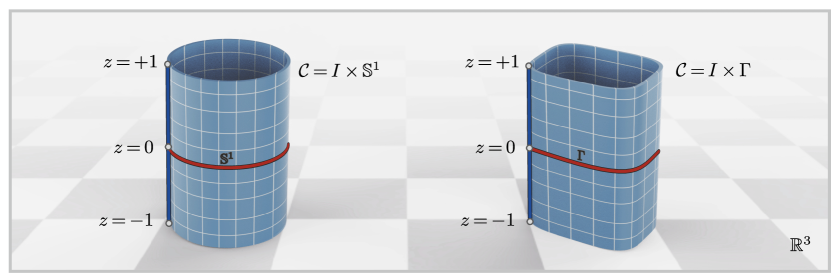
Figure 1. The paper analyzes ground states of the energy functional $\mathcal{E}$ in the admissible class of $\mathbb{S}^{2}$-valued maps defined on cylindrical surfaces $\mathcal{C}=I\times\Gamma$. After a general result on the $z$-invariance of the minimizers of $\mathcal{E}$ in $H^{1}(\mathcal{C},\mathbb{S}^{2})$, we look for the analytic expression of the minimizers in circular cylinders (i.e., in the case $\Gamma=\mathbb{S}^{1}$).

This paper’s main aim concerns the analysis of global minimizers of the energy functional (1.3) in the class of $\mathbb{S}^{2}$-valued maps defined in the circular cylinder $\mathcal{C}=I\times\mathbb{S}^{1}$. The analysis we perform involves several steps.

First, for any $\kappa^{2}>0$, we show that minimizers of the energy $\mathcal{E}$ defined in (1.3) are $z$-invariant. In Proposition 1 we prove the result holds under the more general framework of cylindrical surfaces of the type $\mathcal{C}:=I\times\Gamma$ where $I:=[-1,1]$ and $\Gamma\subseteq\mathbb{R}^{2}$ is the image of a smooth Jordan curve $\zeta:[0,2\pi]\rightarrow\Gamma$ (see Figure 1). Also, we prove that when $\mathcal{C}=I\times\mathbb{S}^{1}$, $z$-invariance of the minimizers holds in the restricted class of weakly axially symmetric configurations which are defined by the condition that

$$\int_{\mathbb{S}^{1}}\boldsymbol{m}_{\bot}(z,\gamma)\mathrm{d}\gamma=0\quad\forall z\in I,$$ (1.4)

where $\boldsymbol{m}_{\bot}:=\boldsymbol{m}-(\boldsymbol{m}\cdot\boldsymbol{e}_{3})\boldsymbol{e}_{3}$. It is simple to show that every axially symmetric configuration satisfies (1.4) (cf. Remark 3). In Theorem 1, we prove that every minimizer of $\mathcal{E}$ in the class of weakly axially symmetric competitors is, in fact, axially symmetric. The proof is based on a symmetrization argument in conjunction with the classical Poincaré-Wirtinger inequality for null average and periodic functions.

Second, we focus on the analysis of global minimizers of the energy $\mathcal{E}$ in the unrestricted class $H^{1}(I\times\mathbb{S}^{1},\mathbb{S}^{2})$, i.e., when no weak axial symmetry is assumed on the competitors. Our main result is a family of sharp Poincaré-type inequalities (see Theorem 2), which allows us to establish the following picture of the energy landscape of $\mathcal{E}$ (see Theorem 3).

1. If $\kappa^{2}\geqslant 3$, the normal vector fields $\pm\boldsymbol{n}$ are the only global minimizers of the energy functional $\mathcal{E}$ in $H^{1}(\mathcal{C},\mathbb{S}^{2})$.

2. Moreover, they are strict local minimizers for every $\kappa^{2}>1$ and unstable for $0<\kappa^{2}<1$. The constant vector fields $\pm\boldsymbol{e}_{3}$ are unstable for all $\kappa^{2}>0$.

The sharp Poincaré-type inequality is stated in Theorem 2 and states that for every $\kappa^{2}>0$ there holds

$$\int_{\mathbb{S}^{1}}\left|\nabla_{\gamma}\boldsymbol{u}\right|^{2}\mathrm{d}\gamma+\kappa^{2}\int_{\mathbb{S}^{1}}|\boldsymbol{u}\times\boldsymbol{n}|^{2}\mathrm{d}\gamma\;\geqslant\;c^{2}_{\kappa}\int_{\mathbb{S}^{1}}|\boldsymbol{u}|^{2}\mathrm{d}\gamma\quad\forall\boldsymbol{u}\in H^{1}(\mathbb{S}^{1},\mathbb{R}^{3}).$$ (1.5)

with $c^{2}_{\kappa}=1$ if $\kappa^{2}\geqslant 3$, $c^{2}_{\kappa}=\frac{1}{2}(\kappa^{2}-\omega_{\kappa}^{2}+4)$ if $0<\kappa^{2}\leqslant 3$, and $\omega_{\kappa}^{2}:=\sqrt{\kappa^{4}+16}$. Our result also includes a precise characterization of the minimizers for which the equality sign is reached in (1.5). For the proof, we work in Fourier space. While the frequencies decouple nicely, the vector-valued nature of $H^{1}(\mathbb{S}^{1},\mathbb{R}^{3})$ elements, as well as the presence of the anisotropic constant $\kappa^{2}$, has the effect that different space directions strongly interact, and this requires careful analysis (see [19]).

Third, motivated by their importance in numerical simulations (see Section 4 for a detailed discussion), we investigate global minimizers of $\mathcal{E}$ in the class of in-plane configurations. We show that if $\boldsymbol{m}_{\bot}\in H^{1}(\mathbb{S}^{1},\mathbb{S}^{1})$ is the profile of a minimizer in $H^{1}(\mathcal{C},\mathbb{S}^{1})$ of the energy functional $\mathcal{E}$, then either $\mathrm{deg\,}\boldsymbol{m}_{\bot}=0$ or $\mathrm{deg\,}\boldsymbol{m}_{\bot}=1$. Indeed, among other things, in Theorem 4 we show the existence of a threshold value $\kappa^{2}_{\ast}$ of the anisotropy parameter for which the following energetic implications hold:

1. If $\kappa^{2}>\kappa_{\ast}^{2}$, then any global minimizer has degree one and, moreover, for every $\kappa^{2}>0$, the normal fields $\pm\boldsymbol{n}$ are the only two minimizers in the homotopy class $\left\{\mathrm{deg\,}\boldsymbol{m}_{\bot}=1\right\}$.

2. If $\kappa^{2}<\kappa_{\ast}^{2}$, then any global minimizer has degree zero, and an accurate analytic description is given in terms of elliptic integrals.

The previous two points allow for a complete characterization of the energy landscape of in-plane minimizers. The normal vector fields $\pm\boldsymbol{n}$ are the only two in-plane energy minimizers when $\kappa^{2}>\kappa_{\ast}^{2}$ and the common minimum value of the energy is $2\pi$. Instead, when $\kappa^{2}<\kappa_{\ast}^{2}$, the minimal energy depends on $\kappa^{2}$, and the precise minimal values, as well as the analytic expressions of the minimizers, are given in terms of elliptic integrals (see (4.8)-(4.9)).

1.3. Outline

The paper is organized as follows. In Section 2 we prove that minimal configurations are $z$-invariant (cf. Proposition 1) and that every minimizer of $\mathcal{E}$ in the class of weakly axially symmetric competitors is, in fact, axially symmetric (cf. Theorem 1). Section 3 is devoted to the analysis of global minimizers of the energy $\mathcal{E}$ in the unrestricted class $H^{1}(I\times\mathbb{S}^{1},\mathbb{S}^{2})$. Our main result is a family of sharp Poincaré-type inequalities (cf. Theorem 2), which allows for establishing a nearly complete picture of the energy landscape of $\mathcal{E}$ (cf. Theorem 3). Finally, in Section 4, we provide a complete characterization of the energy landscape of in-plane minimizers of $\mathcal{E}$.

1.4. Notation

In what follows, for a given embedded submanifold $\mathcal{M}$ of $\mathbb{R}^{3}$, we indicate by $H^{1}(\mathcal{M},\mathbb{R}^{m})$, $m\geqslant 1$, the Sobolev space of vector-valued functions defined on $\mathcal{M}$, endowed with the norm (cf. [1])

$$\|\boldsymbol{u}\|^{2}_{H^{1}(\mathcal{M},\mathbb{R}^{m})}:=\int_{\mathcal{M}}|\boldsymbol{u}(\xi)|^{2}\mathrm{d}\xi+\int_{\mathcal{M}}\left|\nabla_{\xi}\boldsymbol{u}(\xi)\right|^{2}\mathrm{d}\xi\,,$$ (1.6)

where $\nabla_{\xi}\boldsymbol{u}$ is the tangential gradient of $\boldsymbol{u}$ on $\mathcal{M}$. We write $H^{1}(\mathcal{M},\mathbb{S}^{2})$ for the metric subspace of $H^{1}(\mathcal{M},\mathbb{R}^{3})$ consisting of vector-valued functions with values in the unit $2$-sphere of $\mathbb{R}^{3}$. When $\mathcal{M}:=\mathbb{S}^{1}$ is the unit $1$-sphere, $H^{1}(\mathbb{S}^{1},\mathbb{R}^{m})$ identifies to the Sobolev space $H^{1}_{\sharp}([-\pi,\pi],\mathbb{R}^{m})$ consisting of $2\pi$-periodic vector-valued functions and endowed with the norm

$$\|\boldsymbol{u}\|^{2}_{H^{1}_{\sharp}([-\pi,\pi],\mathbb{R}^{m})}:=\int_{-\pi}^{\pi}|\boldsymbol{u}(t)|^{2}\mathrm{d}t+\int_{-\pi}^{\pi}|\partial_{t}\boldsymbol{u}(t)|^{2}\mathrm{d}t.$$ (1.7)

Finally, we denote by $H^{1}_{\sharp}([-\pi,\pi],\mathbb{S}^{1})$ and $H^{1}_{\sharp}([-\pi,\pi],\mathbb{S}^{2})$ the metric subspaces of the Sobolev space $H^{1}_{\sharp}([-\pi,\pi],\mathbb{R}^{m})$ consisting, respectively, of $\mathbb{S}^{1}$-valued and $\mathbb{S}^{2}$-valued periodic functions.

2. Symmetry properties of the minimizers

Our first result, stated in the next Proposition 1, shows that for any $\kappa^{2}>0$ every minimizer $\boldsymbol{m}(z,t)$ of the energy $\mathcal{E}$ in (1.3) is $z$-invariant. We state the result in the more general framework of cylindrical surfaces of the type $\mathcal{C}:=I\times\Gamma$ where $I:=[-1,1]$ and $\Gamma\subseteq\mathbb{R}^{2}$ is the image of a smooth Jordan curve $\zeta:[0,2\pi]\rightarrow\Gamma$. Note that, by parameterizing the cylinder $\mathcal{C}$ through the map

$$\gamma(z,t):=(z,\zeta(t)),$$ (2.1)

we can rewrite the energy functional (1.3) in the form

$$\mathcal{E}(\boldsymbol{m})=\int_{-1}^{1}\int_{\Gamma}\left|\nabla_{\zeta}\boldsymbol{m}(z,\zeta)\right|^{2}+|\partial_{z}\boldsymbol{m}(z,\zeta)|^{2}\mathrm{d}\zeta\mathrm{d}z+\kappa^{2}\int_{-1}^{1}\int_{\Gamma}\,|\boldsymbol{m}(z,\zeta)\times\boldsymbol{n}(\zeta)|^{2}\mathrm{d}\zeta\mathrm{d}z.$$ (2.2)

This equivalent expression of the energy in (1.3) is used in the proof of the following result on the $z$-invariance of energy minimizers.

Proposition 1 ($z$-invariance of energy minimizers).

Let $\boldsymbol{m}\in H^{1}(\mathcal{C},\mathbb{S}^{2})$ be a (global) minimizer of the micromagnetic energy functional (1.3) with $\mathcal{C}:=I\times\Gamma$ and $\Gamma\subseteq\mathbb{R}^{2}$ the image of a smooth Jordan curve $\zeta:[0,2\pi]\rightarrow\Gamma$. Then there exists a minimizer $\boldsymbol{m}_{\ast}\in H^{1}(\mathcal{C},\mathbb{S}^{2})$ of $\mathcal{E}$ in (2.2), built from $\boldsymbol{m}$, which is $z$-invariant, i.e., such that

$$\boldsymbol{m}_{\ast}(z,\zeta)=\boldsymbol{u}_{\ast}(\zeta)$$ (2.3)

for some $\boldsymbol{u}_{\ast}\in H^{1}(\Gamma,\mathbb{S}^{2})$. Actually, every minimizer of $\mathcal{E}$ has the form (2.3) for some minimizer $\boldsymbol{u}_{\ast}\in H^{1}(\Gamma,\mathbb{S}^{2})$ of the reduced energy

$$\mathcal{F}(\boldsymbol{u}):=\int_{\Gamma}\left|\nabla_{\zeta}\boldsymbol{u}(\zeta)\right|^{2}\mathrm{d}\zeta\;+\;\kappa^{2}\int_{\Gamma}|\boldsymbol{u}(\zeta)\times\boldsymbol{n}(\zeta)|^{2}\mathrm{d}\zeta.$$ (2.4)

Remark 1.

In general, $z$-invariance does not hold for critical points of the energy. In fact, when $\mathcal{C}:=I\times\mathbb{S}^{1}$ and $\kappa^{2}=1$, the helices satisfy the Euler–Lagrange equations associated with $\mathcal{E}$ and are not $z$-invariant (cf. Proposition 3). The observation implies that the helical configurations predicted in [44] are critical points of the energy, but not ground states.

Proof.

We use a symmetrization argument. Let $\boldsymbol{m}$ be a minimizer of $\mathcal{E}$, and let us consider the function (note that, $\boldsymbol{n}(z,\zeta)=\boldsymbol{n}(\zeta)$ is $z$-invariant)

$$\Phi:z\in I:=[-1,1]\mapsto\int_{\Gamma}\left|\nabla_{\zeta}\boldsymbol{m}(z,\zeta)\right|^{2}\mathrm{d}\zeta+\kappa^{2}\int_{\Gamma}|\boldsymbol{m}(z,\zeta)\times\boldsymbol{n}(\zeta)|^{2}\mathrm{d}\zeta.$$ (2.5)

In terms of $\Phi$ the energy functional (1.3) reads as

$$\mathcal{E}(\boldsymbol{m})=\int_{-1}^{1}\left(\Phi(z)+\int_{\Gamma}|\partial_{z}\boldsymbol{m}(z,\zeta)|^{2}\mathrm{d}\zeta\right)\mathrm{d}z.$$ (2.6)

Note that since $\boldsymbol{m}$ minimizes $\mathcal{E}$ on the two-dimensional surface $\mathcal{C}$, $\boldsymbol{m}$ is smooth in $\mathcal{C}$. Indeed, the Euler-Lagrange equations for $\boldsymbol{m}$ fit into the class of almost harmonic maps treated in [34, Chapter 4]. In particular, (cf. [34, Theorem 4.2]), $\boldsymbol{m}$ is Hölder continuous and, therefore, by the usual bootstrap argument, smooth in the interior of $\mathcal{C}$. Moreover, through a classical reflection argument (across any of the two boundary components in $\partial\mathcal{C}=\partial I\times\Gamma$) one can easily show that minimizers are smooth up to the boundary. In particular, $\Phi$ is continuous on $[-1,1]$ and $\operatorname{argmin}_{z\in[-1,1]}\Phi(z)\neq\emptyset$. We arbitrarily choose a point $z_{\ast}\in\operatorname{argmin}_{z\in[-1,1]}\Phi(z)$ and, with that, we define the $z$-invariant configuration

$$\boldsymbol{m}_{\ast}(z,\zeta):=\boldsymbol{m}(z_{\ast},\zeta)\quad\text{for every }(z,\zeta)\in I\times\Gamma.$$ (2.7)

Note that, since $\boldsymbol{m}$ is smooth in $\mathcal{C}$, $\boldsymbol{m}_{\ast}$ is well-defined. Taking into account that for every $\xi:=(z,\zeta)\in I\times\Gamma$ we have

$$\left|\nabla_{\xi}\boldsymbol{m}(z,\zeta)\right|^{2}=\left|\nabla_{\zeta}\boldsymbol{m}(z,\zeta)\right|^{2}+|\partial_{z}\boldsymbol{m}(z,\zeta)|^{2}$$ (2.8)

with $\nabla_{\zeta}\boldsymbol{m}$ the tangential gradient on $\zeta$, from (2.2) and (2.5) we get that

$$\mathcal{E}(\boldsymbol{m}_{\ast})=\; \int_{-1}^{1}\int_{\Gamma}\left|\nabla_{\zeta}\boldsymbol{m}_{\ast}(z,\zeta)\right|^{2}\mathrm{d}\zeta\mathrm{d}z+\kappa^{2}\int_{-1}^{1}\int_{\Gamma}|\boldsymbol{m}_{\ast}(z,\zeta)\times\boldsymbol{n}(\zeta)|^{2}\mathrm{d}\zeta\mathrm{d}z$$

$$=\; \int_{-1}^{1}\int_{\Gamma}\left|\nabla_{\zeta}\boldsymbol{m}(z_{\ast},\zeta)\right|^{2}\mathrm{d}\zeta\mathrm{d}z+\kappa^{2}\int_{-1}^{1}\int_{\Gamma}|\boldsymbol{m}(z_{\ast},\zeta)\times\boldsymbol{n}(\zeta)|^{2}\mathrm{d}\zeta\mathrm{d}z$$

$$=\; \int_{-1}^{1}\Phi(z_{\ast})\mathrm{d}z$$

$$\leqslant\; \int_{-1}^{1}\Phi(z)\mathrm{d}z+\int_{-1}^{1}\int_{\Gamma}|\partial_{z}\boldsymbol{m}(z,\zeta)|^{2}\mathrm{d}\zeta\mathrm{d}z$$

$$=\; \mathcal{E}(\boldsymbol{m}).$$ (2.9)

Hence, if $\boldsymbol{m}$ is a minimizer in $H^{1}(\mathcal{C},\mathbb{S}^{2})$ of (1.3) then so is the $z$-invariant configuration $\boldsymbol{m}_{\ast}(z,\zeta):=\boldsymbol{m}(z_{\ast},\zeta)$. Moreover, if $\boldsymbol{m}$ is any minimizer in $H^{1}(\mathcal{C},\mathbb{S}^{2})$, then, with $\boldsymbol{m}_{\ast}$ defined as in (2.7), we get that $\mathcal{E}(\boldsymbol{m}_{\ast})=\mathcal{E}(\boldsymbol{m})$. This entails that all the inequalities in (2.9) are, in fact, equalities. Therefore,

$$\int_{-1}^{1}\int_{\Gamma}|\partial_{z}\boldsymbol{m}(z,\zeta)|^{2}\mathrm{d}\zeta\mathrm{d}z=0,$$ (2.10)

from which we conclude that $\boldsymbol{m}$ is $z$-invariant. This completes the proof. ∎

Since we are interested in the symmetry-breaking phenomena of minimizers, we want to focus on the symmetric case when $\Gamma$ is unit circle $\mathbb{S}^{1}$. Parameterizing the cylinder $\mathcal{C}:=I\times\mathbb{S}^{1}$ through the map

$$\gamma(z,t):=(\cos t)\boldsymbol{e}_{1}+(\sin t)\boldsymbol{e}_{2}+z\boldsymbol{e}_{3},\quad t\in[-\pi,\pi]$$ (2.11)

with $\boldsymbol{e}_{1},\boldsymbol{e}_{2},\boldsymbol{e}_{3}$ the standard basis of $\mathbb{R}^{3}$, we can rewrite (2.2) in the following form

$$\mathcal{E}(\boldsymbol{m})=\int_{-1}^{1}\int_{-\pi}^{\pi}|\partial_{t}\boldsymbol{m}(z,t)|^{2}+|\partial_{z}\boldsymbol{m}(z,t)|^{2}\mathrm{d}t\mathrm{d}z+\kappa^{2}\int_{-1}^{1}\int_{-\pi}^{\pi}|\boldsymbol{m}(z,t)\times\boldsymbol{n}(t)|^{2}\mathrm{d}z\mathrm{d}t$$ (2.12)

where we made the common abuse of notation

$$\boldsymbol{m}(z,t):=(\boldsymbol{m}\circ\gamma)(z,t),\qquad\boldsymbol{n}(t):=(\boldsymbol{n}\circ\gamma)(z,t)=(\cos t,\sin t,0).$$ (2.13)

According to Proposition 1, the energy landscape associated with (1.3) is completely characterized as soon as one describes the minimizers in $H^{1}(\mathbb{S}^{1},\mathbb{S}^{2})$ of the energy functional (cf. (2.4))

$$\mathcal{F}(\boldsymbol{u}):=\int_{\mathbb{S}^{1}}\left|\nabla_{\gamma}\boldsymbol{u}(\gamma)\right|^{2}\mathrm{d}\gamma\;+\;\kappa^{2}\int_{\mathbb{S}^{1}}|\boldsymbol{u}(\gamma)\times\boldsymbol{n}(\gamma)|^{2}\mathrm{d}\gamma.$$ (2.14)

Note that, in terms of the standard (conformal) parameterization of $\mathbb{S}^{1}$ given by $\gamma:t\in[-\pi,\pi]\mapsto(\cos t)\boldsymbol{e}_{1}+(\sin t)\boldsymbol{e}_{2}$, the energy functional $\mathcal{F}$ reads as

$$\mathcal{F}(\boldsymbol{u})=\int_{-\pi}^{\pi}|\partial_{t}\boldsymbol{u}(t)|^{2}\mathrm{d}t+\kappa^{2}\int_{-\pi}^{\pi}|\boldsymbol{u}(t)\times\boldsymbol{n}(t)|^{2}\mathrm{d}t$$ (2.15)

with, again, the convenient abuse of notation

$$\boldsymbol{u}(t):=(\boldsymbol{u}\circ\gamma)(t),\qquad\boldsymbol{n}(t):=(\boldsymbol{n}\circ\gamma)(t)=(\cos t,\sin t,0).$$ (2.16)

For the next result, stated in Proposition 3, we introduce further notation. For each $\boldsymbol{u}\in H^{1}(\mathbb{S}^{1},\mathbb{S}^{2})$ we denote by $\boldsymbol{u}_{\bot}$ the projection of $\boldsymbol{u}$ on $\mathbb{R}^{2}\times\{0\}$, namely, $\boldsymbol{u}_{\bot}:=(u_{1},u_{2},0)$ if $\boldsymbol{u}=(u_{1},u_{2},u_{3})$. Also, we denote by

$$\langle\boldsymbol{u}_{\bot}\rangle:=\frac{1}{2\pi}\int_{-\pi}^{\pi}\boldsymbol{u}_{\bot}(t)\mathrm{d}t$$ (2.17)

the average of $\boldsymbol{u}_{\bot}$ on $\mathbb{S}^{1}$ and, for any $\theta\in[-\pi,\pi]$, we set

$$\boldsymbol{u}_{\theta}(t):=R(t)\left(\begin{array}[]{c}\sin\theta\\ 0\\ \cos\theta\end{array}\right)=(\sin\theta)\boldsymbol{n}+(\cos\theta)\boldsymbol{e}_{3},\qquad R(t):=\left(\begin{array}[]{ccc}\cos t&-\sin t&0\\ \sin t&\cos t&0\\ 0&0&1\end{array}\right).$$ (2.18)

For every $t\in[-\pi,\pi]$ the action of $R(t)$ is a rotation through an angle $t$ about the $z$-axis.

In order to prove Proposition 3 we need the sharp form of the Poincaré-Wirtinger inequality on $\mathbb{S}^{1}$ that we recall here; its proof is a trivial application of Parseval’s theorem for Fourier series and is therefore omitted.

Proposition 2 (Poincaré-Wirtinger inequality).

If $\boldsymbol{u}\in H^{1}_{\sharp}([-\pi,\pi],\mathbb{R}^{2})$ is null-average (i.e., $\langle\boldsymbol{u}_{\bot}\rangle=0$) then

$$\int_{-\pi}^{\pi}|\boldsymbol{u}(t)|^{2}\leqslant\int_{-\pi}^{\pi}|\partial_{t}\boldsymbol{u}(t)|^{2}.$$ (2.19)

The minimizer is reached when $\boldsymbol{u}(t)=\boldsymbol{c}_{1}\cos t+\boldsymbol{c}_{2}\sin t$, for arbitrary constant vectors $\boldsymbol{c}_{1},\boldsymbol{c}_{2}\in\mathbb{R}^{2}$.

We can now state Proposition 3 and Theorem 1, which are our main results about axially symmetric minimizers. Their proof is given at the end of this section.

Proposition 3 (axially symmetric energy minimizers).

In the class of configurations $\boldsymbol{u}\in H^{1}(\mathbb{S}^{1},\mathbb{S}^{2})$ such that $\langle\boldsymbol{u}_{\bot}\rangle=0$, the only global minimizers of (2.14) are given by

$$\left\{\begin{array}[]{llll}\boldsymbol{u}&=&\pm\boldsymbol{e}_{3}&\text{if }0<\kappa^{2}<1,\\ \boldsymbol{u}&=&\boldsymbol{u}_{\theta}&\text{if }\kappa^{2}=1,\\ \boldsymbol{u}&=&\pm\boldsymbol{n}&\text{if }\kappa^{2}>1,\end{array}\right.$$ (2.20)

with $\boldsymbol{u}_{\theta}$ given by (2.18). Thus, if $0<\kappa^{2}<1$ or $\kappa^{2}>1$, there exist only two minimizers, while when $\kappa^{2}=1$ there exist infinitely many minimizers described by $\boldsymbol{u}_{\theta}$ with $\theta$ chosen arbitrarily in $[-\pi,\pi]$. The corresponding values of the minimal energies are given by

$$\left\{\begin{array}[]{ll}2\pi\kappa^{2}&\text{if }0<\kappa^{2}\leqslant 1,\\ 2\pi&\text{if }\kappa^{2}\geqslant 1.\end{array}\right.$$ (2.21)

Remark 2.

Note that at $\kappa^{2}=1$ a symmetry-breaking phenomenon appears. The minimizers suddenly pass from the in-plane configurations $\pm\boldsymbol{n}$ for $\kappa^{2}>1$, to the purely axial configurations $\pm\boldsymbol{e}_{3}$ for $\kappa^{2}<1$. Also, note that if $\boldsymbol{e}\in\mathbb{S}^{1}\times\{0\}$ is in-plane, then $\mathcal{F}(\boldsymbol{e})=\pi\kappa^{2}$. Therefore, for $0<\kappa^{2}<1$, the configurations $\pm\boldsymbol{e}_{3}$ are never global minimizers outside of the restricted admissible class of weakly axially symmetric configurations (i.e., maps $\boldsymbol{u}\in H^{1}(\mathbb{S}^{1},\mathbb{S}^{2})$ such that $\langle\boldsymbol{u}_{\bot}\rangle=0$). A similar observation applies to the configurations $\pm\boldsymbol{n}$ when $0<\kappa^{2}<2$ (because of $\mathcal{F}(\boldsymbol{e})=\pi\kappa^{2}$); in this range of parameters $\pm\boldsymbol{n}$ cannot be global minimizers unless we restrict the minimization problem to the class of axially symmetric configurations.

Before stating our main result on axially symmetric minimizers, we give the following definition. We say that $\boldsymbol{m}\in H^{1}(\mathcal{C},\mathbb{S}^{2})$ is weakly axially symmetric (with respect to the $z$-axis) if

$$\langle\boldsymbol{m}_{\bot}(z,\cdot)\rangle_{\mathbb{S}^{1}}:=\frac{1}{2\pi}\int_{\mathbb{S}^{1}}\boldsymbol{m}_{\bot}(z,\gamma)\mathrm{d}\gamma=0\quad\forall z\in I.$$ (2.22)

Remark 3.

It is important to stress that every axially symmetric configuration satisfies (2.22). Indeed, if $\boldsymbol{m}$ is axially symmetric with respect to the $z$-axis then, in local coordinates, i.e., through the parameterization of $\mathbb{S}^{1}$ given by $\gamma:t\in[-\pi,\pi]\mapsto(\cos t)\boldsymbol{e}_{1}+(\sin t)\boldsymbol{e}_{2}$, we have that

$$\boldsymbol{m}(z,t)=R(t)\tilde{\boldsymbol{m}}(z)\quad\forall(z,t)\in I\times[-\pi,\pi]$$ (2.23)

for some profile $\tilde{\boldsymbol{m}}\in H^{1}(I,\mathbb{S}^{2})$. Hence, $\langle\boldsymbol{m}(z,\cdot)\rangle_{\mathbb{S}^{1}}=(\tilde{\boldsymbol{m}}(z)\cdot\boldsymbol{e}_{3})\boldsymbol{e}_{3}$ for every $z\in I$, and this implies that $\langle\boldsymbol{m}_{\bot}(z,\cdot)\rangle_{\mathbb{S}^{1}}=0$ for every $z\in I$. Also, note that the class of weakly axially symmetric configurations it is not directly related to the class of null-average configurations in $H^{1}(\mathcal{C},\mathbb{S}^{2})$. Even if $\boldsymbol{m}$ is $z$-invariant, (2.22) does not imply that $\boldsymbol{m}$ is null average, but only that its projection $\boldsymbol{m}_{\bot}$ is null average.

Theorem 1 (axially symmetric energy minimizers).

Let $\mathcal{C}:=I\times\mathbb{S}^{1}$, with $I=[-1,1]$. Assume that $\boldsymbol{m}$ is a (global) minimizer of the micromagnetic energy functional (1.3) in the class of weakly axially symmetric configurations. Then, $\boldsymbol{m}$ is $z$-invariant and, more precisely, the following assertions hold:

1. If $0<\kappa^{2}<1$ then necessarily $\boldsymbol{m}\in\{\pm\boldsymbol{e}_{3}\}$.

2. If $\kappa^{2}>1$ then necessarily $\boldsymbol{m}\in\{\pm\boldsymbol{n}\}$.

3. When $\kappa^{2}=1$, there are infinitely many axially symmetric minimizers; they are all $z$-invariant and given by $\boldsymbol{m}(z,t)=\boldsymbol{u}_{\theta}(t)$ with $\theta\in[-\pi,\pi]$ and $\boldsymbol{u}_{\theta}$ given by (2.18).

The values of the minimal energies are given by $4\pi\kappa^{2}$ if $0<\kappa^{2}\leqslant 1$ and by $4\pi$ if $\kappa^{2}\geqslant 1$.

Remark 4.

Note that, due to Remark 3 and the fact that $\pm\boldsymbol{n}$ and $\pm\boldsymbol{e}_{3}$ are axially symmetric (with respect to the $z$-axis), the conclusions of Theorem 1 still hold in the class of axially symmetric minimizers.

Remark 5.

We stress that Theorem 1 does not look for axially symmetric minimizers in the class of minimizers of $\mathcal{E}$. In other words, axially symmetric minimizers do not need to be global minimizers. In fact, Theorem 1 characterizes the minimizers of $\mathcal{E}$ in the class of configurations that satisfy condition (2.22) and shows that, in this class, the minimizers are necessarily $z$-invariant and axially symmetric.

We first give the proof of Proposition 3, then we prove Theorem 1 as a consequence of Proposition 1, Proposition 3, and Remark 3.

Proof.

Proof of Proposition 3. For every $t\in[-\pi,\pi]$ we denote by $R(t)$ the rotation through an angle $t$ about the $z$-axis which appears (cf. (2.18)). Clearly, $\boldsymbol{n}(t)=R(t)\boldsymbol{e}_{1}$. Next, let $\boldsymbol{u}\in H^{1}(\mathbb{S}^{1},\mathbb{S}^{2})$ be a minimizer of (2.15) and let us choose $t_{\ast}\in[-\pi,\pi]$ such that

$$t_{\ast}\in\underset{t\in[-\pi,\pi]}{\arg\>\min}\left(|\boldsymbol{u}_{\bot}(t)|^{2}+\kappa^{2}|\boldsymbol{u}(t)\times\boldsymbol{n}(t)|^{2}\right)$$ (2.24)

with $\boldsymbol{u}_{\bot}(t):=(u_{1}(t),u_{2}(t),0)$. Here, we are identifying $\boldsymbol{u}$ with its Hölder continuous representative so that $t_{\ast}$ is well-defined. Define the new configuration

$$\boldsymbol{u}^{\ast}(t):=R(t)R^{\top}(t_{\ast})\boldsymbol{u}(t_{\ast}).$$ (2.25)

We then have $|\boldsymbol{u}^{\ast}(t)|=1$ and $\langle\boldsymbol{u}^{\ast}_{\bot}\rangle=0$ because $\left\langle R(t)R^{\top}(t_{\ast})\boldsymbol{u}(t_{\ast})\right\rangle=(\boldsymbol{u}(t_{\ast})\cdot\boldsymbol{e}_{3})\boldsymbol{e}_{3}$. Moreover,

$$|\partial_{t}\boldsymbol{u}^{\ast}(t)|^{2}\;=\;\left|R^{\top}\partial_{t}R(t)R^{\top}(t_{\ast})\boldsymbol{u}(t_{\ast})\right|^{2}\;=\;\left|\boldsymbol{e}_{3}\times\left(R^{\top}(t_{\ast})\boldsymbol{u}(t_{\ast})\right)\right|^{2}\;=\;|\boldsymbol{u}_{\bot}(t_{\ast})|^{2}$$ (2.26)

and

$$|\boldsymbol{u}^{\ast}(t)\times\boldsymbol{n}(t)|^{2}\;=\;\left|R^{\top}(t_{\ast})\boldsymbol{u}(t_{\ast})\times\boldsymbol{e}_{1}\right|^{2}\;=\;\;|\boldsymbol{u}(t_{\ast})\times\boldsymbol{n}(t_{\ast})|^{2}$$ (2.27)

It follows that

$$\mathcal{F}(\boldsymbol{u}^{\ast})=\; \int_{-\pi}^{\pi}|\partial_{t}\boldsymbol{u}^{\ast}(t)|^{2}\mathrm{d}t+\kappa^{2}\int_{-\pi}^{\pi}|\boldsymbol{u}^{\ast}(t)\times\boldsymbol{n}(t)|^{2}\;\mathrm{d}t$$ (2.28)

$$=\; \int_{-\pi}^{\pi}|\boldsymbol{u}_{\bot}(t_{\ast})|^{2}+\kappa^{2}|\boldsymbol{u}(t_{\ast})\times\boldsymbol{n}(t_{\ast})|^{2}\;\mathrm{d}t$$ (2.29)

$$\leqslant\; \int_{-\pi}^{\pi}|\boldsymbol{u}_{\bot}(t)|^{2}+\kappa^{2}|\boldsymbol{u}(t)\times\boldsymbol{n}(t)|^{2}\;\mathrm{d}t.$$ (2.30)

After that, the sharp Poincaré-Wirtinger inequality on $\mathbb{S}^{1}$ (cf. Proposition 2) assures that for every $\boldsymbol{u}_{\bot}\in H^{1}(\mathbb{S}^{1},\mathbb{R}^{2})$ such that $\langle\boldsymbol{u}_{\bot}\rangle=\boldsymbol{0}$ one has

$$\int_{-\pi}^{\pi}|\boldsymbol{u}_{\bot}(t)|^{2}\;\mathrm{d}t\leqslant\int_{-\pi}^{\pi}|\partial_{t}\boldsymbol{u}_{\bot}(t)|^{2}\mathrm{d}t.$$ (2.31)

Combining (2.30) and (2.31) we conclude that

$$\mathcal{F}(\boldsymbol{u}^{\ast})\leqslant\int_{-\pi}^{\pi}|\partial_{t}\boldsymbol{u}_{\bot}(t)|^{2}+\kappa^{2}|\boldsymbol{u}(t)\times\boldsymbol{n}(t)|^{2}\;\mathrm{d}t\;\leqslant\;\mathcal{F}(\boldsymbol{u}).$$ (2.32)

Thus $\boldsymbol{u}^{\ast}$ and $\boldsymbol{u}$ are both minimizers. This implies that

$$\mathcal{F}(\boldsymbol{u})=\int_{-\pi}^{\pi}|\partial_{t}\boldsymbol{u}_{\bot}(t)|^{2}+\kappa^{2}|\boldsymbol{u}(t)\times\boldsymbol{n}(t)|^{2}\;\mathrm{d}t=\mathcal{F}(\boldsymbol{u}^{\ast}).$$ (2.33)

It follows that whenever $\langle\boldsymbol{u}_{\bot}\rangle=\boldsymbol{0}$, then necessarily $\partial_{t}(\boldsymbol{u}(t)\cdot\boldsymbol{e}_{3})=0$ on $\mathbb{S}^{1}$. On the other hand, the equality $\mathcal{F}(\boldsymbol{u}^{\ast})=\mathcal{F}(\boldsymbol{u})$ also entails that the equality sign is reached in the sharp Poincaré-Wirtinger inequality (2.19), i.e., that

$$\int_{-\pi}^{\pi}|\boldsymbol{u}_{\bot}(t)|^{2}\mathrm{d}t=\int_{-\pi}^{\pi}|\partial_{t}\boldsymbol{u}_{\bot}(t)|^{2}\mathrm{d}t$$ (2.34)

whenever $\boldsymbol{u}$ is a minimizer with $\langle\boldsymbol{u}_{\bot}\rangle=\boldsymbol{0}$. However, the equality sign in the Poincaré-Wirtinger inequality is achieved if, and only if, $\boldsymbol{u}_{\bot}=(\cos t)\boldsymbol{a}_{1}+(\sin t)\boldsymbol{a}_{2}$ for some $\boldsymbol{a}_{1},\boldsymbol{a}_{2}\in\mathbb{R}^{2}\times\{0\}$. Combining this observation with the conditions $\partial_{t}(\boldsymbol{u}(t)\cdot\boldsymbol{e}_{3})=0$ and $|\boldsymbol{u}|=1$ we conclude that if $\langle\boldsymbol{u}_{\bot}\rangle=\boldsymbol{0}$ then necessarily

$$\boldsymbol{u}(t)=\boldsymbol{u}_{\theta}(t):=\left(\begin{array}[]{c}\sin\theta\cos t\\ \sin\theta\sin t\\ \cos\theta\end{array}\right)$$ (2.35)

for some $\theta\in\mathbb{R}$. Finally, we note that with $\boldsymbol{u}(t)$ given by the previous expression, we have

$$|\partial_{t}\boldsymbol{u}_{\theta}(t)|^{2}=\sin^{2}\theta,\qquad|\boldsymbol{u}_{\theta}(t)\times\boldsymbol{n}(t)|^{2}=1-\sin^{2}\theta.$$

Therefore

$$\mathcal{F}(\boldsymbol{u}_{\theta}(t))=\int_{-\pi}^{\pi}\sin^{2}\theta+\kappa^{2}(1-\sin^{2}\theta)\mathrm{d}t\;=\;2\pi[\kappa^{2}+\sin^{2}\theta(1-\kappa^{2})].$$ (2.36)

Minimizing (2.36) with respect to $\theta\in[-\pi,\pi]$ we get that $\theta=\pm\pi$ when $0<\kappa^{2}<1$ and, in this case,

$$\mathcal{F}(\boldsymbol{u}_{\theta}(t))=\mathcal{F}(\pm\boldsymbol{e}_{3})=2\pi\kappa^{2}.$$ (2.37)

Also, we get that the angle $\theta$ can be arbitrarily chosen when $\kappa^{2}=1$, and in this case,

$$\mathcal{F}(\boldsymbol{u}_{\theta}(t))=2\pi\quad\forall\theta\in[-\pi,\pi].$$ (2.38)

Finally, we obtain that $\theta=\pm\pi/2$ when $\kappa^{2}>1$ and, in this case,

$$\mathcal{F}(\boldsymbol{u}_{\theta}(t))=2\pi.$$ (2.39)

This gives (2.20) and completes the proof. ∎

Proof.

Proof of Theorem 1 The proof is a consequence of Proposition 1, Proposition 3, and Remark 3. The only point is to realize that the proof of Proposition 1 is not affected by the introduction of the additional weakly axially symmetric constraint (2.22). Indeed, the only place where the constraint (2.22) impacts the proof of Proposition 1 is in the regularity of minimizers which we based on [34, Theorem 4.2], and one can show that the linearity of the constraint (2.22) makes the arguments in [34, Theorem 4.2] still work. However, for the reader’s convenience, we give here an alternative proof of Proposition 1 that does not rely on the theory developed in [34, Chapter 4] and immediately adapts to the presence of the additional constraint (2.22). This will complete the proof of Theorem 1.

Proof of Proposition 1 under the additional constraint (2.22). We assume that $\mathbb{S}^{1}=\zeta([0,2\pi])$ is parameterized by arc-length. Let $\boldsymbol{m}_{0}$ be a minimizer of

$$\mathcal{E}\left(\boldsymbol{m}\right)=\int_{-1}^{1}\int_{0}^{2\pi}\left|\nabla\boldsymbol{m}(z,t)\right|^{2}+\kappa^{2}|\boldsymbol{m}(z,t)\times\boldsymbol{n}(t)|^{2}\mathrm{d}z\mathrm{d}t,$$

and let $\boldsymbol{m}_{\varepsilon}\in C^{\infty}\left(I\times\Gamma,\mathbb{S}^{2}\right)$ be such that $\boldsymbol{m}_{\varepsilon}\rightarrow\boldsymbol{m}_{0}$ in $H^{1}\left(I\times\Gamma,\mathbb{S}^{2}\right)$ (see [38, p.267]).  For every $\varepsilon>0$ we consider the function (which now depends on $\varepsilon$)

$$\Phi_{\varepsilon}:z\in I:=[-1,1]\mapsto\int_{0}^{2\pi}\left|\partial_{t}\boldsymbol{m}_{\varepsilon}(z,t)\right|^{2}\mathrm{d}t+\kappa^{2}|\boldsymbol{m}_{\varepsilon}(z,t)\times\boldsymbol{n}(t)|^{2}\mathrm{d}t.$$ (2.40)

In terms of $\Phi_{\varepsilon}$ the energy reads as

$$\mathcal{E}(\boldsymbol{m}_{\varepsilon})=\int_{-1}^{1}\left(\Phi_{\varepsilon}(z)+\int_{0}^{2\pi}|\partial_{z}\boldsymbol{m}_{\varepsilon}(z,t)|^{2}\mathrm{d}t\right)\mathrm{d}z.$$ (2.41)

For every $\varepsilon>0$, $\Phi_{\varepsilon}$ is continuous on $[-1,1]$ and $\operatorname{argmin}_{z\in[-1,1]}\Phi_{\varepsilon}(z)\neq\emptyset$. We arbitrarily choose a point $z_{\varepsilon}\in\operatorname{argmin}_{z\in[-1,1]}\Phi_{\varepsilon}(z)$ and, with that, we define the $z$-invariant configuration $\boldsymbol{u}_{\varepsilon}(t):=\boldsymbol{m}_{\varepsilon}(z_{\varepsilon},t)$. We then have

$$\mathcal{E}(\boldsymbol{u}_{\varepsilon})=\hskip 2.70004pt \int_{-1}^{1}\int_{0}^{2\pi}\left|\partial_{t}\boldsymbol{m}_{\varepsilon}(z_{\varepsilon},t)\right|^{2}\mathrm{d}t+\kappa^{2}|\boldsymbol{m}_{\varepsilon}(z_{\varepsilon},t)\times\boldsymbol{n}(t)|^{2}\mathrm{d}t\mathrm{d}z$$

$$=\hskip 2.70004pt \int_{-1}^{1}\Phi_{\varepsilon}(z_{\varepsilon})\mathrm{d}t\leqslant\int_{-1}^{1}\Phi_{\varepsilon}(z)\mathrm{d}z\leqslant\int_{-1}^{1}\left(\Phi_{\varepsilon}(z)+\int_{0}^{2\pi}|\partial_{z}\boldsymbol{m}_{\varepsilon}(z,t)|^{2}\mathrm{d}t\right)\mathrm{d}z$$

$$=\hskip 2.70004pt \mathcal{E}(\boldsymbol{m}_{\varepsilon}).$$ (2.42)

Since $\mathcal{E}(\boldsymbol{m}_{\varepsilon})$ is bounded, we have that $\boldsymbol{u}_{\varepsilon}$ is bounded in $H^{1}(I_{2\pi},\mathbb{R}^{3})$, $I_{2\pi}:=(0,2\pi)$, and, therefore, there exists $\boldsymbol{u}_{0}\in H^{1}(I_{2\pi},\mathbb{R}^{3})$ such that $\boldsymbol{u}_{\varepsilon}\rightharpoonup\boldsymbol{u}_{0}$ weakly in $H^{1}(I_{2\pi},\mathbb{R}^{3})$ and, up to a subsequence, $|\boldsymbol{u}_{0}|=1$ (this is because of $\boldsymbol{u}_{\varepsilon}(t):=\boldsymbol{m}_{\varepsilon}(z_{\varepsilon},t)$ with $\left|\boldsymbol{m}_{\varepsilon}\right|=1$). Passing to the limit, we then have that

$$\mathcal{E}(\boldsymbol{u}_{0})\leqslant\liminf_{\varepsilon\rightarrow 0}\mathcal{E}(\boldsymbol{u}_{\varepsilon})\leqslant\int_{-1}^{1}\Phi_{0}(z)\mathrm{d}z\leqslant\int_{-1}^{1}\left(\Phi_{0}(z)+\int_{0}^{2\pi}|\partial_{z}\boldsymbol{m}_{0}(z,t)|^{2}\mathrm{d}t\right)\mathrm{d}z=\mathcal{E}(\boldsymbol{m}_{0}).$$

Hence, by the minimality of $\boldsymbol{m}_{0}$ we have that $\mathcal{E}(\boldsymbol{u}_{0})=\mathcal{E}(\boldsymbol{m}_{0})$ and, therefore,

$$\int_{-1}^{1}\int_{0}^{2\pi}|\partial_{z}\boldsymbol{m}_{0}(z,t)|^{2}\mathrm{d}t\mathrm{d}z=0,$$ (2.43)

from which we conclude that $\boldsymbol{m}_{0}$ is $z$-invariant. This completes the proof when constraint (2.22) is not present. Note that although we assumed that $\Gamma=\mathbb{S}^{1}$, the proof works for general smooth Jordan curves $\Gamma$ with minor notational modifications.

The same proof now works even if we assume the weakly axially symmetric constraint (2.22). Indeed, if $\boldsymbol{m}_{0}^{\bot}$ is a weakly axially symmetric minimizer, then also $\boldsymbol{u}_{0}^{\bot}$ is weakly axially symmetric. To see this, we observe that

$$\left|\int_{0}^{2\pi}\boldsymbol{u}_{\varepsilon}^{\bot}(t)-\boldsymbol{m}_{\varepsilon}^{\bot}(z,t)\mathrm{d}t\right| =\left|\int_{0}^{2\pi}\boldsymbol{m}_{\varepsilon}^{\bot}(z_{\varepsilon},t)-\boldsymbol{m}_{\varepsilon}^{\bot}(z,t)\mathrm{d}t\right|$$

$$=\left|\int_{0}^{2\pi}\int_{z}^{z_{\varepsilon}}\partial_{z}\boldsymbol{m}_{\varepsilon}^{\bot}(s,t)\mathrm{d}s\mathrm{d}t-\int_{z}^{z_{\varepsilon}}\partial_{z}\left(\int_{0}^{2\pi}\boldsymbol{m}_{0}^{\bot}(s,t)\mathrm{d}s\right)\mathrm{d}t\right|$$

$$=\left|\int_{0}^{2\pi}\int_{z}^{z_{\varepsilon}}\partial_{z}\boldsymbol{m}_{\varepsilon}^{\bot}(s,t)\mathrm{d}s\mathrm{d}t-\int_{0}^{2\pi}\int_{z}^{z_{\varepsilon}}\partial_{z}\boldsymbol{m}_{0}^{\bot}(s,t)\mathrm{d}s\mathrm{d}t\right|$$

$$\leqslant\int_{0}^{2\pi}\int_{-1}^{1}\left|\partial_{z}\left(\boldsymbol{m}_{\varepsilon}^{\bot}-\boldsymbol{m}_{0}^{\bot}\right)\right|\mathrm{d}s\mathrm{d}t,$$ (2.44)

and, therefore, passing to the limit for $\varepsilon\rightarrow 0$, we get that

$$\left|\int_{0}^{2\pi}\boldsymbol{u}_{0}^{\bot}(t)-\boldsymbol{m}_{0}^{\bot}(z,t)\mathrm{d}t\right|=0,$$ (2.45)

i.e., $\langle\boldsymbol{u}_{0}^{\bot}\rangle_{\mathbb{S}^{1}}=\left\langle\boldsymbol{m}_{0}^{\bot}(z,\cdot)\right\rangle_{\mathbb{S}^{1}}=\mathbf{0}$. This completes the proof. ∎

3. Global minimizers. A sharp Poincaré-type inequality on the cylinder

An exact characterization of the minimizers of the energy functional (1.3) is a nontrivial task. Qualitative aspects of the energy landscape have been investigated in [44] through numerical simulations. However, sometimes it is enough to obtain a meaningful lower bound on the energy to gain information on the ground states. For that, we relax the constraint from $\boldsymbol{m}$ being $\mathbb{S}^{2}$-valued to the following energy constraint:

$$\frac{1}{4\pi}\int_{\mathcal{C}}|\boldsymbol{m}|^{2}=1,$$ (3.1)

with $\mathcal{C}:=I\times\mathbb{S}^{1}$ and $I:=[-1,1]$. From the physical point of view, this type of relaxation corresponds to a passage from classical physics to a probabilistic quantum mechanics perspective, and it has been proved to be useful in obtaining nontrivial lower bounds of the ground state micromagnetic energy (see, e.g., [8, 13, 19]). From the mathematical perspective, replacing the pointwise constraint $|\boldsymbol{m}|=1$ a.e. in $\mathcal{C}$ with (3.1) frames the minimization problem in the context of Poincaré-type inequalities, where sometimes the relaxed problem can be solved exactly, and the dependence of the minimizers on the geometrical and physical properties of the model made explicit. This relaxation can help to obtain sufficient conditions for minimizers to have specific geometric structures (see, e.g., [8, 13, 19]). We note that the pointwise constraint $|\boldsymbol{m}|=1$ a.e. in $\mathcal{C}$ is equivalent to the following two energy constraints in terms of the $L^{2}$ and $L^{4}$ norms:

$$\frac{1}{4\pi}\int_{\mathcal{C}}|\boldsymbol{m}|^{2}=1,\qquad\frac{1}{4\pi}\int_{\mathcal{C}}|\boldsymbol{m}|^{4}=1.$$ (3.2)

Indeed, by Cauchy–Schwarz inequality $4\pi=(|\boldsymbol{m}|^{2},1)_{L^{2}(\mathcal{C})}\leqslant\||\boldsymbol{m}|^{2}\|_{L^{2}(\mathcal{C})}\|1\|_{L^{2}(\mathcal{C})}=4\pi$, which assures that the equality sign in the previous estimate is reached only when $|\boldsymbol{m}|^{2}$ is constant and, therefore, necessarily equal to $1$. It follows that the relaxed problem can also be interpreted as the one obtained by forgetting about the $L^{4}$ constraint.

Our results include the precise characterization of the minimal value and global minimizers of the energy functional $\mathcal{E}$ defined in (1.3) on the space of $H^{1}(\mathcal{C},\mathbb{R}^{3})$ vector fields satisfying the relaxed constraint (3.1). Thanks to Proposition 1, we can focus on the analysis of the minimizers in $H^{1}(\mathbb{S}^{1},\mathbb{R}^{3})$ of the normalized energy functional

$$\mathcal{G}(\boldsymbol{u}):=\frac{1}{2\pi}\int_{\mathbb{S}^{1}}\left|\nabla_{\gamma}\boldsymbol{u}\right|^{2}\mathrm{d}\gamma\;+\;\frac{\kappa^{2}}{2\pi}\int_{\mathbb{S}^{1}}|\boldsymbol{u}\times\boldsymbol{n}|^{2}\mathrm{d}\gamma,$$ (3.3)

subject to the $L^{2}$-constraint

$$\frac{1}{2\pi}\int_{\mathbb{S}^{1}}|\boldsymbol{u}|^{2}\mathrm{d}\gamma=1.$$ (3.4)

Clearly, every minimizer of (3.3) in $H^{1}(\mathbb{S}^{1},\mathbb{S}^{2})$ satisfies the constraint (3.4) and provides an upper bound to the minimal energy associated with the problem (3.3)-(3.4). Thus, problem (3.3)-(3.4) is a relaxed version of the minimization problem for $\mathcal{G}$ in $H^{1}(\mathbb{S}^{1},\mathbb{S}^{2})$. Although the expression of the energy functional (3.3) is, up to the constant factor $\frac{1}{2\pi}$, the same as of $\mathcal{F}$ in (2.14), we denoted it by $\mathcal{G}$ to stress that it is part of the relaxed minimization problem.

The existence of minimizers of the problem (3.3)-(3.4) quickly follows by direct methods in the Calculus of Variations. However, uniqueness is out of the question due to the energy’s invariance under the orthogonal group and reflections. Indeed, for every $\kappa^{2}>0$, at least two minimizers always exist because if $\boldsymbol{u}$ is a minimizer of $\mathcal{G}$, also $-\boldsymbol{u}$ minimizes $\mathcal{G}$. We only focus on the nontrivial case $\kappa^{2}\neq 0$; otherwise, constant configurations $\boldsymbol{\sigma}\in\mathbb{S}^{2}$ are the only minimizers.

In what follows, we denote by $\boldsymbol{n}$ the outward normal vector field to $\mathbb{S}^{1}$ and by $\boldsymbol{\tau}:=\nabla_{\gamma}\boldsymbol{n}$ the tangential one. When we refer to the local coordinates representation of a configuration $\boldsymbol{u}_{\bot}\in H^{1}(\mathbb{S}^{1},\mathbb{R}^{3})$, it is always meant the curve $\boldsymbol{u}_{\bot}\circ\gamma$, with $\gamma:t\in[-\pi,\pi]\mapsto(\cos t)e_{1}+(\sin t)e_{2}$, and $t\in[-\pi,\pi]$. Thus, e.g., in local coordinates, we have that $\boldsymbol{\tau}(t)=(-\sin t,\cos t)$ and $\boldsymbol{n}(t)=(\cos t,\sin t)$.

Our main result includes the precise characterization of the minimal value and global minimizers of the relaxed problem (3.3)-(3.4) on the space of $H^{1}(\mathbb{S}^{1},\mathbb{R}^{3})$. In fact, we establish the following sharp Poincaré-type inequality in $H^{1}(\mathbb{S}^{1},\mathbb{R}^{3})$.

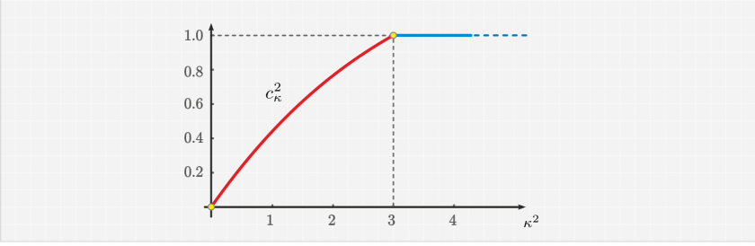
Figure 2. The graph of the optimal Poincaré constant $c^{2}_{\kappa}$ as a function of the parameter $\kappa^{2}$. The optimal constant $c^{2}_{\kappa}$ increases until the saturation value $c^{2}_{\kappa}=1$ is reached at $\kappa^{2}=3$.

Theorem 2 (sharp Poincaré-type inequality in $H^{1}(\mathbb{S}^{1},\mathbb{R}^{3})$).

For every $\kappa^{2}>0$ the following sharp Poincaré-type inequality holds,

$$\int_{\mathbb{S}^{1}}\left|\nabla_{\gamma}\boldsymbol{u}\right|^{2}\mathrm{d}\gamma+\kappa^{2}\int_{\mathbb{S}^{1}}|\boldsymbol{u}\times\boldsymbol{n}|^{2}\mathrm{d}\gamma\hskip 2.70004pt\geqslant\hskip 2.70004ptc^{2}_{\kappa}\int_{\mathbb{S}^{1}}|\boldsymbol{u}|^{2}\mathrm{d}\gamma\quad\forall\boldsymbol{u}\in H^{1}(\mathbb{S}^{1},\mathbb{R}^{3}),$$ (3.5)

where the best Poincaré constant $c^{2}_{\kappa}$ is the continuous function of $\kappa$ given by

$$c_{\kappa}^{2}:=\left\{\begin{array}[]{lll}1&\text{if }&\kappa^{2}\geqslant 3,\\ \frac{1}{2}(\kappa^{2}-\omega_{\kappa}^{2}+4)&\text{if }&0<\kappa^{2}\leqslant 3,\end{array}\right.$$ (3.6)

with $\omega_{\kappa}^{2}:=\sqrt{\kappa^{4}+16}$. Moreover, the equality sign in the Poincaré inequality (3.5) is reached if, and only if, $\boldsymbol{u}\in H^{1}(\mathbb{S}^{1},\mathbb{R}^{3})$ has the following expressions:

1. If $\kappa^{2}>3$, the equality sign in (3.5) is reached only by the normal vector fields $\pm\boldsymbol{n}$.

2. If $\kappa^{2}=3$, the equality is reached if, and only if, $\boldsymbol{u}$ is an element of the family represented in local coordinates by

   $$\boldsymbol{u}_{\bot}(t)=\sqrt{2}\rho_{1}\cos(\theta+t)\boldsymbol{\tau}(t)+\left[\pm\sqrt{1-5\rho_{1}^{2}}+2\sqrt{2}\rho_{1}\sin(\theta+t)\right]\boldsymbol{n}(t)$$ (3.7)

   for arbitrary $\theta\in[-\pi,\pi]$ and $0\leqslant\rho_{1}\leqslant 1/\sqrt{5}$. In particular ($\rho_{1}=0$), the normal vector fields $\pm\boldsymbol{n}$ persist as minimizers for $\kappa^{2}=3$.

3. If $0<\kappa^{2}<3$, the equality sign in (3.5) is reached by any element of the family represented in local coordinates by

   $$\boldsymbol{u}_{\bot}(t)=\sqrt{2}(\sin\phi_{\kappa})\cos(\theta+t)\boldsymbol{\tau}(t)+\sqrt{2}(\cos\phi_{\kappa})\sin(\theta+t)\boldsymbol{n}(t),$$ (3.8)

   with $\theta\in[-\pi,\pi]$ arbitrary, and $\phi_{\kappa}\in[0,\pi/2]$ given by

   $$\phi_{\kappa}=\frac{1}{2}\arctan(4/\kappa^{2}).$$ (3.9)

   Moreover, there are no $\mathbb{S}^{2}$-valued configurations for which the equality sign is achieved in (3.5).

The normal fields $\pm\boldsymbol{n}$ are universal configurations as their energy does not depend on $\kappa^{2}$.

Remark 6.

In view of our original problem concerning $\mathbb{S}^{2}$-valued minimizers, we note that setting $\rho_{1}=0$ in (3.7) we recover the normal vector fields $\pm\boldsymbol{n}$, and these are the only $\mathbb{S}^{2}$-valued minimizers of the problem (3.3)-(3.4) when $\kappa^{2}=3$. Instead, when $0<\kappa^{2}<3$, there are no $\mathbb{S}^{2}$-valued configurations for which the equality sign is achieved in (3.5).

A graph of the optimal Poincaré constant $c^{2}_{\kappa}$ as a function of $\kappa^{2}$ is depicted in Figure 2. Figure 3represents a plot of the minimal configurations in (3.7) for which the equality sign is attained in the Poincaré inequality when $\kappa^{2}=3$. Also, a plot of the minimal vector fields in (3.8) is given in Figure 4 for different values of $0<\kappa^{2}<3$.

Before giving the proof of Theorem 2, we want to point out some of its consequences.

Proposition 4.

For every $\kappa^{2}>0$, the map

$$\boldsymbol{u}\in H^{1}(\mathbb{S}^{1},\mathbb{R}^{3})\mapsto\left(\int_{\mathbb{S}^{1}}\left|\nabla_{\gamma}\boldsymbol{u}\right|^{2}\mathrm{d}\gamma+\kappa^{2}|\boldsymbol{u}\times\boldsymbol{n}|^{2}\mathrm{d}\gamma\right)^{1/2}$$

is a norm on $H^{1}(\mathbb{S}^{1},\mathbb{R}^{3})$ equivalent to the classical norm

$$\|\boldsymbol{u}\|_{H^{1}(\mathbb{S}^{1},\mathbb{R}^{3})}=\left(\int_{\mathbb{S}^{1}}\left|\nabla_{\gamma}\boldsymbol{u}\right|^{2}\mathrm{d}\gamma+|\boldsymbol{u}|^{2}\mathrm{d}\gamma\right)^{1/2}.$$

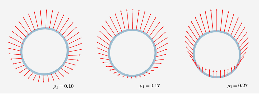
Figure 3. A plot of the minimal configurations in (3.7) for which the equality sign is attained in the Poincaré inequality when $\kappa^{2}=3$. The optimal vector fields are represented for three different values of $\rho_{1}$. From left to right, we plot (3.7) for $\rho_{1}=0.10$, $\rho_{1}=0.17$ and $\rho_{1}=0.27$.

Next, by Theorem 2 we get that for $\kappa^{2}\geqslant 3$ the relaxed minimization problem (3.3)-(3.4) admits $\mathbb{S}^{2}$-valued minimizers. Thus, as a byproduct of Theorem 2, we obtain the following characterization of micromagnetic ground states in thin cylindrical shells.

Theorem 3 (Micromagnetic ground states in thin cylindrical shells).

For every value $\kappa^{2}>0$ of the anisotropy, the normal vector fields $\pm\boldsymbol{n}$, as well as the constant vector fields $\pm\boldsymbol{e}_{3}$ are stationary points of the micromagnetic energy functional (cf. (1.3))

$$\mathcal{E}\left(\boldsymbol{m}\right)=\int_{\mathcal{C}}\left|\nabla_{\xi}\boldsymbol{m}\right|^{2}\mathrm{d}\xi+\kappa^{2}\int_{\mathcal{C}}|\boldsymbol{m}\times\boldsymbol{n}|^{2}\mathrm{d}\xi,\quad\boldsymbol{m}\in H^{1}(\mathcal{C},\mathbb{S}^{2}),$$

and the following properties hold:

1. If $\kappa^{2}\geqslant 3$, the normal vector fields $\pm\boldsymbol{n}$ are the only global minimizers of the energy functional $\mathcal{E}$ in $H^{1}(\mathcal{C},\mathbb{S}^{2})$. Also, they are locally stable for every $\kappa^{2}\geqslant 1$ and unstable for $0<\kappa^{2}<1$. Moreover, when $\kappa^{2}>1$, the normal vector fields $\pm\boldsymbol{n}$ are local minimizers of the energy $\mathcal{E}$.

2. The constant vector fields $\pm\boldsymbol{e}_{3}$ are unstable for all $\kappa^{2}>0$.

Remark 7.

Although the constant vector fields $\pm\boldsymbol{e}_{3}$ are unstable for all $\kappa^{2}>0$, they are stable in the class of axially symmetric minimizers, as has been shown in Theorem 1.

Figure 4. A plot of the minimal vector fields in (3.8) for which the equality sign is attained in the Poincaré inequality when $0<\kappa^{2}<3$. From left to right, we plot (3.8) for $\kappa^{2}=0.1$, $\kappa^{2}=1$, and $\kappa^{2}=2.5$.

Proof.

In coordinates, the energy functional (cf. (2.4)) reads as

$$\mathcal{F}(\boldsymbol{m})=\int_{-1}^{1}\int_{-\pi}^{\pi}\left|\nabla\boldsymbol{m}\right|^{2}+\kappa^{2}\left|\boldsymbol{m}\times\boldsymbol{n}\right|^{2}\hskip 1.69998pt\mathrm{d}t\,\mathrm{d}z,$$ (3.10)

with $\boldsymbol{m}\in H^{1}(\mathcal{C},\mathbb{S}^{2})$ and $\nabla=(\partial_{z},\partial_{t})$. The Euler-Lagrange associated with $\mathcal{F}$ read as

$$-\Delta\boldsymbol{m}-\kappa^{2}(\boldsymbol{m}\cdot\boldsymbol{n})\boldsymbol{n}=\lambda(t)\boldsymbol{m},\qquad\lambda(t)=|\nabla\boldsymbol{m}|^{2}-\kappa^{2}(\boldsymbol{m}\cdot\boldsymbol{n})^{2}.$$ (3.11)

It is therefore clear that $\boldsymbol{m}(t)=\pm\boldsymbol{e}_{3}$ and $\boldsymbol{m}(t)=\pm\boldsymbol{n}(t)$ are critical points of the above energy. Let us investigate their stability. The second variation of $\mathcal{F}$ is given by

$$\mathcal{F}^{\prime\prime}(\boldsymbol{m})(\boldsymbol{\varphi})=\int_{-1}^{1}\int_{-\pi}^{\pi}|\nabla\boldsymbol{\varphi}|^{2}-\kappa^{2}(\boldsymbol{\varphi}\cdot\boldsymbol{n})^{2}-(|\nabla\boldsymbol{m}|^{2}-\kappa^{2}(\boldsymbol{m}\cdot\boldsymbol{n})^{2})|\boldsymbol{\varphi}|^{2}\mathrm{d}t\,\mathrm{d}z,$$ (3.12)

and is defined on all $\boldsymbol{\varphi}\in H^{1}\cap L^{\infty}(\mathcal{C},\mathbb{R}^{3})$ such that $\boldsymbol{\varphi}\cdot\boldsymbol{m}\equiv 0$ in $\mathcal{C}$.

Proof of i. It is clear from Theorem 2 that $\pm\boldsymbol{n}$ are the only global minimizers of $\mathcal{F}$ whenever $\kappa^{2}\geqslant 3$. It remains to analyze their stability in the range $0<\kappa^{2}<3$. For that, it is sufficient to evaluate the second variation at $\boldsymbol{m}=\pm\boldsymbol{n}$, which reads as

$$\mathcal{F}^{\prime\prime}(\pm\boldsymbol{n})(\boldsymbol{\varphi})=\int_{-1}^{1}\int_{-\pi}^{\pi}|\nabla\boldsymbol{\varphi}|^{2}+(\kappa^{2}-1)|\boldsymbol{\varphi}|^{2}\mathrm{d}t\,\mathrm{d}z.$$ (3.13)

Setting $\boldsymbol{\varphi}=\boldsymbol{e}_{3}$ we obtain that $\mathcal{F}^{\prime\prime}(\pm\boldsymbol{n})(\boldsymbol{e}_{3})=4\pi(\kappa^{2}-1)$. Therefore the normal vector fields $\pm\boldsymbol{n}$ are unstable critical points of $\mathcal{F}$ when $\kappa^{2}<1$.

However, (3.13) shows that for $\kappa^{2}>1$ we have uniform local stability of the critical points $\pm\boldsymbol{n}$. We want to show that $\pm\boldsymbol{n}$ are, in fact, local minimizers of the energy functional $\mathcal{F}$. We focus on $+\boldsymbol{n}$, the argument for $-\boldsymbol{n}$ being the same. Following [19], first, we compute the finite variation of $\mathcal{F}$ corresponding to an admissible increment $\boldsymbol{v}$ of $\boldsymbol{n}$, i.e., $\boldsymbol{v}\in H^{1}(\mathcal{C},\mathbb{R}^{3})$ such that $\left|\boldsymbol{n}+\boldsymbol{v}\right|=1$ in $\mathcal{C}$. A simple computation gives

$$\mathcal{F}(\boldsymbol{n}+\boldsymbol{v})-\mathcal{F}(\boldsymbol{n})=\int_{-1}^{1}\int_{-\pi}^{\pi}\left|\nabla\boldsymbol{v}\right|^{2}+\kappa^{2}\left(\left|\boldsymbol{v}\right|^{2}-(\boldsymbol{v}\cdot\boldsymbol{n})^{2}\right)-\left|\boldsymbol{v}\right|^{2}\hskip 1.69998pt\mathrm{d}t\,\mathrm{d}z.$$ (3.14)

Next, we define $\boldsymbol{\varphi}=\boldsymbol{v}-(\boldsymbol{v}\cdot\boldsymbol{n})\boldsymbol{n}$ and want to rewrite the previous expression in $\boldsymbol{\varphi}$. Since $\boldsymbol{v}=\boldsymbol{\varphi}+(\boldsymbol{v}\cdot\boldsymbol{n})\boldsymbol{n}$ we have $\partial_{t}\boldsymbol{v}=\partial_{t}\boldsymbol{\varphi}+(\boldsymbol{v}\cdot\boldsymbol{n})\boldsymbol{\tau}+\left(\partial_{t}(\boldsymbol{v}\cdot\boldsymbol{n})\right)\boldsymbol{n}$ with $\boldsymbol{\tau}:=\partial_{t}\boldsymbol{n}$. Using that $\partial_{t}\boldsymbol{\varphi}\cdot\boldsymbol{n}=-\boldsymbol{\varphi}\cdot\boldsymbol{\tau}$ because of $\boldsymbol{\varphi}\cdot\boldsymbol{n}=0$, we obtain

$$|\partial_{t}\boldsymbol{v}|^{2}=|\partial_{t}\boldsymbol{\varphi}|^{2}+(\boldsymbol{v}\cdot\boldsymbol{n})^{2}+\left|\partial_{t}(\boldsymbol{v}\cdot\boldsymbol{n})\right|^{2}+2(\partial_{t}\boldsymbol{\varphi}\cdot\boldsymbol{\tau})(\boldsymbol{v}\cdot\boldsymbol{n})-2(\boldsymbol{\varphi}\cdot\boldsymbol{\tau})\partial_{t}(\boldsymbol{v}\cdot\boldsymbol{n}).$$ (3.15)

Integrating by parts the previous relation, we infer that

$$\int_{-1}^{1}\int_{-\pi}^{\pi}|\partial_{t}\boldsymbol{v}|^{2}\mathrm{d}t\mathrm{d}z=\int_{-1}^{1}\int_{-\pi}^{\pi}|\partial_{t}\boldsymbol{\varphi}|^{2}+(\boldsymbol{v}\cdot\boldsymbol{n})^{2}+\left|\partial_{t}(\boldsymbol{v}\cdot\boldsymbol{n})\right|^{2}+4(\partial_{t}\boldsymbol{\varphi}\cdot\boldsymbol{\tau})(\boldsymbol{v}\cdot\boldsymbol{n})\mathrm{d}t\,\mathrm{d}z.$$ (3.16)

Similarly, we have

$$|\partial_{z}\boldsymbol{\varphi}|^{2}=\left|\partial_{z}\boldsymbol{v}-(\partial_{z}\boldsymbol{v}\cdot\boldsymbol{n})\boldsymbol{n}\right|^{2}=|\partial_{z}\boldsymbol{v}|^{2}-\left|\partial_{z}\left(\boldsymbol{v}\cdot\boldsymbol{n}\right)\right|^{2}.$$ (3.17)

Hence, plugging the previous expression into (3.14), using that $|\boldsymbol{\varphi}|^{2}=|\boldsymbol{v}|^{2}-(\boldsymbol{v}\cdot\boldsymbol{n})^{2}$, and taking into account (3.13), we obtain

$$\mathcal{F}(\boldsymbol{n}+\boldsymbol{v})-\mathcal{F}(\boldsymbol{n}) = \int_{-1}^{1}\int_{-\pi}^{\pi}\left|\nabla\boldsymbol{v}\right|^{2}+\kappa^{2}|\boldsymbol{\varphi}|^{2}-\left|\boldsymbol{v}\right|^{2}\hskip 1.69998pt\mathrm{d}t\,\mathrm{d}z$$ (3.18)

$$\overset{\eqref{eq:exprdzf2rev}}{=} \int_{-1}^{1}\int_{-\pi}^{\pi}|\nabla\boldsymbol{\varphi}|^{2}+(\kappa^{2}-1)|\boldsymbol{\varphi}|^{2}+\left|\nabla(\boldsymbol{v}\cdot\boldsymbol{n})\right|^{2}+4(\partial_{t}\boldsymbol{\varphi}\cdot\boldsymbol{\tau})(\boldsymbol{v}\cdot\boldsymbol{n})\mathrm{d}t\,\mathrm{d}z$$

$$\overset{\eqref{eq:secvarF}}{=} \mathcal{F}^{\prime\prime}(\boldsymbol{n})(\boldsymbol{\varphi})+\int_{-1}^{1}\int_{-\pi}^{\pi}\left|\nabla(\boldsymbol{v}\cdot\boldsymbol{n})\right|^{2}+4(\partial_{t}\boldsymbol{\varphi}\cdot\boldsymbol{\tau})(\boldsymbol{v}\cdot\boldsymbol{n})\mathrm{d}t\,\mathrm{d}z.$$

Note that since $-2\boldsymbol{v}\cdot\boldsymbol{n}=|\boldsymbol{v}|^{2}$ and $\boldsymbol{v}=\boldsymbol{\varphi}+(\boldsymbol{v}\cdot\boldsymbol{n})\boldsymbol{n}$ we have that $|\boldsymbol{v}|^{2}=|\boldsymbol{\varphi}|^{2}+\frac{1}{4}|\boldsymbol{v}|^{4}$. Overall, from the previous considerations and (3.18), we obtain that

$$\mathcal{F}(\boldsymbol{n}+\boldsymbol{v})-\mathcal{F}(\boldsymbol{n}) \;=\;\mathcal{F}^{\prime\prime}(\boldsymbol{n})(\boldsymbol{\varphi})+\int_{-1}^{1}\int_{-\pi}^{\pi}\left|\nabla(\boldsymbol{v}\cdot\boldsymbol{n})\right|^{2}-2(\partial_{t}\boldsymbol{\varphi}\cdot\boldsymbol{\tau})|\boldsymbol{v}|^{2}\mathrm{d}t\,\mathrm{d}z$$

$$\;\geqslant\;\mathcal{F}^{\prime\prime}(\boldsymbol{n})(\boldsymbol{\varphi})-\int_{-1}^{1}\int_{-\pi}^{\pi}\left(2|\boldsymbol{v}|^{4}+\frac{1}{2}|\partial_{t}\boldsymbol{\varphi}|^{2}\right)\mathrm{d}t\,\mathrm{d}z$$

$$\;\geqslant\;\frac{1}{2}\|\nabla\boldsymbol{\varphi}\|_{L^{2}(\mathcal{C})}^{2}+(\kappa^{2}-1)\|\boldsymbol{v}\|_{L^{2}(\mathcal{C})}^{2}-\left(2+\frac{\kappa^{2}-1}{4}\right)\|\boldsymbol{v}\|_{L^{4}(\mathcal{C})}^{4}.$$ (3.19)

Now we use Gagliardo–Nirenberg inequality (see, e.g., [21]), i.e., the existence of a positive constant $c_{L}>0$ such that $\|\boldsymbol{v}\|_{L^{4}(\mathcal{C})}^{4}\leqslant c_{L}\|\boldsymbol{v}\|_{H^{1}(\mathcal{C})}^{2}\|\boldsymbol{v}\|_{L^{2}(\mathcal{C})}^{2}$ for every $\boldsymbol{v}\in H^{1}(\mathcal{C},\mathbb{R}^{3})$. Therefore

$$\mathcal{F}(\boldsymbol{n}+\boldsymbol{v})-\mathcal{F}(\boldsymbol{n})\;\geqslant\;\frac{1}{2}\|\nabla\boldsymbol{\varphi}\|_{L^{2}(\mathcal{C})}^{2}+\left[(\kappa^{2}-1)-c_{L}\left(2+\frac{\kappa^{2}-1}{4}\right)\|\boldsymbol{v}\|_{H^{1}(\mathcal{C})}^{2}\right]\|\boldsymbol{v}\|_{L^{2}(\mathcal{C})}^{2}.$$ (3.20)

To conclude, we observe that for a given $\kappa^{2}>1$ the previous right-hand side is nonnegative as soon as $\|\boldsymbol{v}\|_{H^{1}(\mathcal{C})}^{2}$ is chosen small enough.

Proof of ii. Testing the second variation at $\boldsymbol{m}=\pm\boldsymbol{e}_{3}$ against $\boldsymbol{v}=\boldsymbol{e}_{1}$ we obtain

$$\mathcal{F}^{\prime\prime}(\pm\boldsymbol{e}_{3})(\boldsymbol{e}_{1})=-\kappa^{2}\int_{-1}^{1}\int_{-\pi}^{\pi}(\boldsymbol{e}_{1}\cdot\boldsymbol{n})^{2}\mathrm{d}t\,\mathrm{d}z=-2\pi\kappa^{2}<0.$$ (3.21)

Therefore we know that the constant $\mathbb{S}^{2}$-valued vector fields $\boldsymbol{m}=\pm\boldsymbol{e}_{3}$ are unstable for all $\kappa^{2}>0$. ∎

Remark 8.

As already pointed out in the introduction, there are several analogies in the behavior of the minimizers of the micromagnetic energy in cylindrical and spherical surfaces. However, there are also remarkable differences. Indeed, in both cases, the normal vector fields are the unique global minimizers of the energy functional in a wide range of parameters [19]. However, the topological consequences are very different. On the one hand, the normal vector fields $\pm\boldsymbol{n}_{\mathbb{S}^{2}}$ to $\mathbb{S}^{2}$ carry a different skyrmion number because $\mathrm{deg\,}\left(\pm\boldsymbol{n}_{\mathbb{S}^{2}}\right)=\pm 1$, and, by Hopf theorem [33], they cannot be homotopically mapped from one to the other. This translates into the so-called topological protection of the ground states. On the other hand, due to the odd dimension, the two normal vector fields $\pm\boldsymbol{n}$ to $\mathbb{S}^{1}$ have the same degree, and therefore, they can be “easily” switched from one to the other through appropriate external fields.

Remark 9.

The result of Theorem 3 can be interpreted in terms of the size of the magnetic particle. Indeed, a simple rescaling of the energy functional (1.3) shows that the range $\kappa^{2}\geqslant 3$ corresponds to the geometric regime of cylindrical magnets with a large radius. This is the dual version of Brown’s fundamental theorem on $3d$ fine ferromagnetic particles, which shows the existence of a critical diameter below which the unique energy minimizers are the constant-in-space magnetizations [8, 13, 4].

3.1. Proof of the sharp Poincaré inequality (Theorem 2)

To prove Theorem 2, we need the following result which, in particular, shows that the constant vector field $\boldsymbol{e}_{3}\in\mathbb{S}^{2}$ is never a global minimizer of the relaxed minimization problem (3.3)-(3.4). In fact, any critical point of $\mathcal{G}$ with energy strictly less than $\kappa^{2}$ (in particular, any minimizer) is in-plane.

Lemma 1.

Let $\kappa^{2}\neq 0$. Any critical point $\boldsymbol{u}\in H^{1}(\mathbb{S}^{1},\mathbb{R}^{3})$ of the relaxed problem (3.3)-(3.4) satisfying the energy bound $\mathcal{G}(\boldsymbol{u})<\kappa^{2}$ is in-plane, i.e.,

$$\boldsymbol{u}(\gamma)\cdot\boldsymbol{e}_{3}=0\quad\forall\gamma\in\mathbb{S}^{1}.$$ (3.22)

Moreover, the minimal energy satisfies the energy bounds

$$0<\mathcal{G}(\boldsymbol{u})\leqslant\min\left\{\frac{\kappa^{2}}{2},1\right\}.$$ (3.23)

In particular, every minimizer of the relaxed problem (3.3)-(3.4) is in-plane.

Proof.

In terms of the standard parameterization of the unit circle $\mathbb{S}^{1}$, the problem reduces to the minimization, in the Sobolev space of periodic functions $H^{1}_{\sharp}([-\pi,\pi],\mathbb{R}^{3})$, of the energy functional

$$\mathcal{G}(\boldsymbol{u}):=\frac{1}{2\pi}\int_{-\pi}^{\pi}|\partial_{t}\boldsymbol{u}|^{2}\mathrm{d}t\;+\;\frac{\kappa^{2}}{2\pi}\int_{-\pi}^{\pi}|\boldsymbol{u}\times\boldsymbol{n}|^{2}\mathrm{d}t,$$ (3.24)

subject to the constraint

$$\frac{1}{2\pi}\int_{-\pi}^{\pi}|\boldsymbol{u}|^{2}\mathrm{d}t=1.$$ (3.25)

We start observing that as soon as $\kappa^{2}\neq 0$ the minimal energy is strictly positive. Indeed, if $\mathcal{G}(\boldsymbol{u})=0$, then one gets at the same time $\boldsymbol{u}=\boldsymbol{n}$ and $\boldsymbol{u}:=\boldsymbol{\sigma}$ for some $\boldsymbol{\sigma}\in\mathbb{S}^{2}$ (because of the constraint (3.25)). Thus $\mathcal{G}(\boldsymbol{u})>0$ for every $\boldsymbol{u}\in H^{1}_{\sharp}([-\pi,\pi],\mathbb{R}^{3})$ satisfying the constraint (3.25). In fact, the minimum in the class of constant $\mathbb{S}^{2}$-valued configurations is reached by any element of the class of in-plane uniform fields, i.e., by any configuration $\boldsymbol{\sigma}\in\mathbb{S}^{2}$ such that $\boldsymbol{\sigma}\cdot\boldsymbol{e}_{3}=0$. The common minimum value in this class being

$$\mathcal{G}(\boldsymbol{\sigma})=\frac{\kappa^{2}}{2\pi}\int_{-\pi}^{\pi}|\boldsymbol{\sigma}|^{2}-(\boldsymbol{\sigma}\cdot\boldsymbol{n})^{2}\mathrm{d}t=\frac{\kappa^{2}}{2}>0.$$ (3.26)

Also, note that since $|\partial_{t}\boldsymbol{n}|^{2}=1$ we have $\mathcal{G}(\boldsymbol{n})=1$ regardless of the value of $\kappa$. Therefore, if $\boldsymbol{u}$ is a minimum point of the relaxed minimization problem (3.24)-(3.25) then

$$0<\mathcal{G}(\boldsymbol{u})\leqslant\min\left\{\frac{\kappa^{2}}{2},1\right\}.$$ (3.27)

This proves (3.23).

Next, we consider the Euler–Lagrange equations associated with the relaxed minimization problem (3.24)-(3.25). A direct computation yields that if $\boldsymbol{u}\in H^{1}_{\sharp}([-\pi,\pi],\mathbb{R}^{3})$ is a minimizer, then it satisfies the equations

$$-\partial_{tt}\boldsymbol{u}+\kappa^{2}(\boldsymbol{u}-(\boldsymbol{n}\otimes\boldsymbol{n})\boldsymbol{u})=\lambda\boldsymbol{u}\quad\text{in }\left(H^{1}_{\sharp}([-\pi,\pi],\mathbb{R}^{3})\right)^{\prime},\quad\frac{1}{2\pi}\int_{-\pi}^{\pi}|\boldsymbol{u}|^{2}\mathrm{d}t=1,$$ (3.28)

for some Lagrange multiplier $\lambda\in\mathbb{R}$. To ease notation, we write the Euler-Lagrange equations (3.28) in their (distributional) form; however, behind the scenes, we always mean the associated weak formulation in $H^{1}_{\sharp}([-\pi,\pi],\mathbb{R}^{3})$. To get (3.28) it is sufficient to note that in $H^{1}_{\sharp}([-\pi,\pi],\mathbb{R}^{3})$ one has

$$|\boldsymbol{u}\times\boldsymbol{n}+\varepsilon\boldsymbol{\varphi}\times\boldsymbol{n}|^{2}-|\boldsymbol{u}\times\boldsymbol{n}|^{2}+\mathcal{O}(\varepsilon^{2})=\; 2\varepsilon(\boldsymbol{u}\times\boldsymbol{n})\cdot(\boldsymbol{\varphi}\times\boldsymbol{n})$$ (3.29)

$$=\; 2\varepsilon\boldsymbol{\varphi}\cdot(\boldsymbol{u}-(\boldsymbol{n}\otimes\boldsymbol{n})\boldsymbol{u}).$$ (3.30)

To get an explicit expression of the Lagrange multiplier $\lambda\in\mathbb{R}$ we dot multiply by $\boldsymbol{u}$ both members of (3.28). Taking into account the constraint (3.25), we get that

$$\frac{1}{2\pi}\int_{-\pi}^{\pi}|\partial_{t}\boldsymbol{u}|^{2}+\kappa^{2}(|\boldsymbol{u}|^{2}-(\boldsymbol{u}_{\bot}\cdot\boldsymbol{n})^{2})\mathrm{d}t=\frac{\lambda}{2\pi}\int_{-\pi}^{\pi}|\boldsymbol{u}|^{2}\mathrm{d}t,$$ (3.31)

from which the relation $\lambda=\mathcal{G}(\boldsymbol{u})$ follows. Combining this observation with (3.23), we get that if $\boldsymbol{u}$ is a minimizer of the constrained minimization problem (3.24)-(3.25) then necessarily

$$0<\lambda\equiv\mathcal{G}(\boldsymbol{u})\leqslant\min\left\{\frac{\kappa^{2}}{2},1\right\}.$$ (3.32)

To conclude the proof it is sufficient to prove that every solution $\boldsymbol{u}$ of the Euler–Lagrange equations (3.28) such that $\mathcal{G}(\boldsymbol{u})<\kappa^{2}$ is an in-plane configuration. For that, we dot multiply by $\boldsymbol{e}_{3}$ on both sides of (3.28) to get the relation

$$\partial_{tt}u_{3}=\mu\cdot u_{3},\quad\text{with }\mu=\kappa^{2}-|\lambda|.$$ (3.33)

Note that $\mu=|\mu|>0$ whenever $\boldsymbol{u}$ satisfies the energy bound $\mathcal{G}(\boldsymbol{u})<\kappa^{2}$. In this case, the general solution of the previous equation is given by

$$u_{3}(t):=c_{1}e^{t\sqrt{|\mu|}}+c_{2}e^{-t\sqrt{|\mu|}},\quad c_{1},c_{2}\in\mathbb{R}.$$ (3.34)

The only periodic solution of the previous equation is the zero solution. Therefore, any critical point $\boldsymbol{u}\in H^{1}_{\sharp}([-\pi,\pi],\mathbb{R}^{3})$ of the problem (3.24)-(3.25) satisfying the energy bound $\mathcal{G}(\boldsymbol{u})<\kappa^{2}$ is in-plane. In particular, because of (3.32), any minimizer of the problem (3.24)-(3.25) is in-plane. This concludes the proof. ∎

Proof.

Proof of Theorem 2. To deduce the sharp Poincaré inequality (3.5) one has to solve the minimization problem for $\mathcal{G}$ given by (3.3)-(3.4). Indeed, let $\boldsymbol{u}_{\ast}\in H^{1}(\mathbb{S}^{1},\mathbb{R}^{3})$ be a minimizer of $\mathcal{G}$ in the class of vector fields $\boldsymbol{u}\in H^{1}(\mathbb{S}^{1},\mathbb{R}^{3})$ that satisfy the $L^{2}$-constraint $\|\boldsymbol{u}\|^{2}_{L^{2}(\mathbb{S}^{1},\mathbb{R}^{3})}=2\pi$, and set $c^{2}_{\kappa}:=\mathcal{G}(\boldsymbol{u}_{\ast})$. For every $\boldsymbol{v}\in H^{1}(\mathbb{S}^{1},\mathbb{R}^{3})\setminus\{0\}$ the configuration

$$\boldsymbol{u}:=\sqrt{2\pi}\frac{\boldsymbol{v}}{\|\boldsymbol{v}\|_{L^{2}(\mathbb{S}^{1},\mathbb{R}^{3})}}$$ (3.35)

is an admissible competitor of the minimization problem for $\mathcal{G}$ in (3.3)-(3.4). Therefore

$$\mathcal{G}(\boldsymbol{u})=\frac{1}{\|\boldsymbol{v}\|_{L^{2}(\mathbb{S}^{1},\mathbb{R}^{3})}^{2}}\left(\int_{\mathbb{S}^{1}}\left|\nabla_{\gamma}\boldsymbol{v}\right|^{2}\mathrm{d}\gamma+\kappa^{2}\int_{\mathbb{S}^{1}}|\boldsymbol{v}\times\boldsymbol{n}|^{2}\mathrm{d}\gamma\right)\geqslant\mathcal{G}(\boldsymbol{u}_{\ast})=c_{\kappa}^{2}.$$ (3.36)

Multiplying all sides of the previous relation by $\|\boldsymbol{v}\|_{L^{2}(\mathbb{S}^{1},\mathbb{R}^{3})}^{2}$ we get the sharp Poincaré inequality (3.5) with $c^{2}_{\kappa}$ being the minimal energy of $\mathcal{G}$ subject to (3.4). The equality sign is achieved by any minimizer of the relaxed problem for $\mathcal{G}$ in (3.3)-(3.4).

According to Lemma 1, it is possible to restrict our attention to the class of vector fields in $\boldsymbol{u}_{\bot}\in H^{1}(\mathbb{S}^{1},\mathbb{R}^{2})$ satisfying the $L^{2}$-constraint

$$\frac{1}{2\pi}\int_{\mathbb{S}^{1}}|\boldsymbol{u}_{\bot}|^{2}\mathrm{d}\gamma=1,$$ (3.37)

and the minimization problem (3.3)-(3.4) reduces to the minimization of

$$\mathcal{G}(\boldsymbol{u}_{\bot}):=\frac{1}{2\pi}\int_{\mathbb{S}^{1}}\left|\nabla_{\gamma}\boldsymbol{u}_{\bot}\right|^{2}\mathrm{d}\gamma+\frac{\kappa^{2}}{2\pi}\int_{\mathbb{S}^{1}}(|\boldsymbol{u}_{\bot}|^{2}-(\boldsymbol{u}_{\bot}\cdot\boldsymbol{n})^{2})\mathrm{d}\gamma$$ (3.38)

in $H^{1}_{\sharp}(\mathbb{S}^{1},\mathbb{R}^{2})$ subject to the constraint (3.37). To solve this minimization problem, we use Fourier analysis, and we work in local coordinates, i.e., in $H^{1}_{\sharp}([-\pi,\pi],\mathbb{R}^{2})$. Note that, in local coordinates, the Euler–Lagrange equations (3.28) simplify to

$$\partial_{tt}\boldsymbol{u}_{\bot}+\kappa^{2}(\boldsymbol{n}\otimes\boldsymbol{n})\boldsymbol{u}_{\bot}=|\mu|\boldsymbol{u}_{\bot},\qquad|\mu|:=\kappa^{2}-|\lambda|>\frac{\kappa^{2}}{2}.$$ (3.39)

We consider the moving orthonormal frame of $\mathbb{R}^{2}$ given by $(\boldsymbol{\tau},\boldsymbol{n})$, with both $\boldsymbol{\tau}:=\partial_{t}\boldsymbol{n}$ and $\boldsymbol{n}\in C^{\infty}_{\sharp}([-\pi,\pi],\mathbb{R}^{2})$. More explicitly, we have $\boldsymbol{\tau}(t)=(-\sin t,\cos t)$ and $\boldsymbol{n}(t)=(\cos t,\sin t)$. Then, we set

$$\boldsymbol{u}_{\bot}=u_{1}\boldsymbol{\tau}+u_{2}\boldsymbol{n}$$ (3.40)

with $u_{1}:=\boldsymbol{u}_{\bot}\cdot\boldsymbol{\tau}$ and $u_{2}:=\boldsymbol{u}_{\bot}\cdot\boldsymbol{n}$. Note that both $u_{1}$ and $u_{2}$ belong to $H^{1}_{\sharp}([-\pi,\pi],\mathbb{R})$.

In this moving frame, the energy (3.38) assumes the expression

$$\mathcal{G}(\boldsymbol{u}_{\bot})=\frac{1}{2\pi}\int_{-\pi}^{\pi}(\partial_{t}u_{1}(t)+u_{2}(t))^{2}+(\partial_{t}u_{2}(t)-u_{1}(t))^{2}+\kappa^{2}u_{1}^{2}(t)\mathrm{d}t$$ (3.41)

and the constraint (3.37) reads as

$$\frac{1}{2\pi}\int_{-\pi}^{\pi}u_{1}^{2}(t)+u_{2}^{2}(t)\mathrm{d}t=1.$$ (3.42)

In what follows, we denote by $\dot{\ell}_{2}(\mathbb{Z},\mathbb{C}^{2})$ the Sobolev space of square summable sequences $(\boldsymbol{c}_{n})_{n\in\mathbb{Z}}:=(c_{1,n},c_{2,n})_{n\in\mathbb{Z}}$ in $\ell_{2}(\mathbb{Z},\mathbb{C}^{2})$ such that $(n\boldsymbol{c}_{n})_{n\in\mathbb{Z}}$ is still in $\ell_{2}(\mathbb{Z},\mathbb{C}^{2})$. Every in-plane vector field $\boldsymbol{u}_{\bot}\in H^{1}_{\sharp}([-\pi,\pi],\mathbb{R}^{2})$, with components $u_{1}:=\boldsymbol{u}_{\bot}\cdot\boldsymbol{\tau}$ and $u_{2}:=\boldsymbol{u}_{\bot}\cdot\boldsymbol{n}$, can then be represented in Fourier series as follows

$$u_{1}(t)=\sum_{n\in\mathbb{Z}}c_{1,n}e^{int},\qquad u_{2}(t)=\sum_{n\in\mathbb{Z}}c_{2,n}e^{int},$$ (3.43)

for some $(\boldsymbol{c}_{n})_{n\in\mathbb{Z}}:=(c_{1,n},c_{2,n})_{n\in\mathbb{Z}}\in\dot{\ell}_{2}(\mathbb{Z},\mathbb{C}^{2})$ and with $i$ the imaginary unit. As a side remark, we note that

$$\langle\boldsymbol{u}_{\bot}\rangle=\langle u_{1}\boldsymbol{\tau}\rangle+\langle u_{2}\boldsymbol{n}\rangle=\sum_{n\in\{\pm 1\}}\langle c_{1,n}e^{int}\boldsymbol{\tau}\rangle+\sum_{n\in\{\pm 1\}}\langle c_{2,n}e^{int}\boldsymbol{n}\rangle.$$ (3.44)

Therefore, the information on the average of $\boldsymbol{u}_{\bot}$ is contained in the harmonics of order $|n|=1$.

Next, we represent the energy functional $\mathcal{G}$ given by (3.41), in the Fourier domain. For that, we use Parseval’s theorem to restate the energy $\mathcal{G}$ in (3.41) in terms of Fourier coefficients as follows

$$\mathcal{G}(\boldsymbol{u}_{\bot})=\sum_{n\in\mathbb{Z}}(n^{2}+1)(|c_{1,n}|^{2}+|c_{2,n}|^{2})+\kappa^{2}|c_{1,n}|^{2}-4n\Im[c_{1,n}\overline{c_{2,n}}].$$

Also, we take advantage of the symmetry properties of the complex Fourier coefficients. Indeed, since we are representing real-valued functions, we know that for every $n\in\mathbb{N}$ there holds

$$c_{1,0},c_{2,0}\in\mathbb{R},\quad c_{1,-n}=\overline{c_{1,n}},\quad c_{2,-n}=\overline{c_{2,n}}.$$ (3.45)

After that, the energy $\mathcal{G}(\boldsymbol{u}_{\bot})$ can be represented under the form

$$\mathcal{G}(\boldsymbol{u}_{\bot}) =(|c_{1,0}|^{2}+|c_{2,0}|^{2})+\kappa^{2}|c_{1,0}|^{2}$$

$$\quad+2\sum_{n\geqslant 1}(n^{2}+1)(|c_{1,n}|^{2}+|c_{2,n}|^{2})+\kappa^{2}|c_{1,n}|^{2}-4n\Im[c_{1,n}\overline{c_{2,n}}].$$ (3.46)

We would like to interpret the previous expression as an energy functional on $\dot{\ell}_{2}(\mathbb{Z}_{\geq 0},\mathbb{R}^{2}\times\mathbb{R}^{2})$. For that, we first observe that $\Im[c_{1,n}\overline{c_{2,n}}]=J(\Re[c_{2,n}],\Im[c_{2,n}])\cdot(\Re[c_{1,n}],\Im[c_{1,n}])$ with the antisymmetric matrix

$$J:=\left(\begin{array}[]{cc}0&-1\\ 1&0\end{array}\right)$$ (3.47)

representing the unitary image in matrix form, and then we set

$$\boldsymbol{c}_{1,0}=\left(\begin{array}[]{c}c_{1,0}\\ 0\end{array}\right),\boldsymbol{c}_{2,0}=\left(\begin{array}[]{c}c_{2,0}\\ 0\end{array}\right),$$ (3.48)

$$\boldsymbol{c}_{1,n}=\sqrt{2}\left(\begin{array}[]{c}\Re[c_{1,n}]\\ \Im[c_{1,n}]\end{array}\right),\boldsymbol{c}_{2,n}=\sqrt{2}\left(\begin{array}[]{c}\Re[c_{2,n}]\\ \Im[c_{2,n}]\end{array}\right)\quad n\geqslant 1.$$ (3.49)

In this way, the minimization problem (3.41)-(3.42) for $\mathcal{G}$ is equivalent to the minimization (in the space of sequences $\dot{\ell}_{2}(\mathbb{Z}_{\geq 0},\mathbb{R}^{2}\times\mathbb{R}^{2})$) of the energy functional

$$\mathcal{G}(\boldsymbol{u}_{\bot})=\sum_{n\geqslant 0}(n^{2}+1)(|\boldsymbol{c}_{1,n}|^{2}+|\boldsymbol{c}_{2,n}|^{2})+\kappa^{2}|\boldsymbol{c}_{1,n}|^{2}-4nJ\boldsymbol{c}_{2,n}\cdot\boldsymbol{c}_{1,n}$$ (3.50)

with $\boldsymbol{c}_{1,0}\cdot\boldsymbol{e}_{2}=\boldsymbol{c}_{2,0}\cdot\boldsymbol{e}_{2}=0$, and subject to the constraint

$$\sum_{n\geqslant 0}|\boldsymbol{c}_{1,n}|^{2}+|\boldsymbol{c}_{2,n}|^{2}=1.$$ (3.51)

If $(\boldsymbol{c}_{1,n},\boldsymbol{c}_{2,n})$ minimizes the energy (3.50)-(3.51), then the Euler-Lagrange equations associated with the minimization problem gives the existence of a Lagrange multiplier $\lambda\in\mathbb{R}$ such that for every $n\geqslant 0$ there holds

$$(n^{2}+1)\boldsymbol{c}_{1,n}+\kappa^{2}\boldsymbol{c}_{1,n}-2nJ\boldsymbol{c}_{2,n} =\lambda\boldsymbol{c}_{1,n},$$ (3.52)

$$(n^{2}+1)\boldsymbol{c}_{2,n}+2nJ\boldsymbol{c}_{1,n} =\lambda\boldsymbol{c}_{2,n}.$$ (3.53)

from which one easily gets that $\lambda=\mathcal{G}(\boldsymbol{u}_{\bot})$. Therefore the previous two relations can be rewritten under the form

$$\left(n^{2}+1+\kappa^{2}-\mathcal{G}(\boldsymbol{u}_{\bot})\right)\boldsymbol{c}_{1,n} =2nJ\boldsymbol{c}_{2,n}$$ (3.54)

$$\left(n^{2}+1-\mathcal{G}(\boldsymbol{u}_{\bot})\right)\boldsymbol{c}_{2,n} =-2nJ\boldsymbol{c}_{1,n}.$$ (3.55)

Note that for $n=0$, the first of the previous two relations gives $\left(1+\kappa^{2}-\mathcal{G}(\boldsymbol{u}_{\bot})\right)c_{1,0}=0$ and, therefore, by (3.32) we have

$$c_{1,0}=0.$$ (3.56)

Also, observe that (3.32) assures that for every $n\geqslant 0$ there holds

$$\left(n^{2}+1+\kappa^{2}-\mathcal{G}(\boldsymbol{u}_{\bot})\right)>0,\qquad\left(n^{2}+1-\mathcal{G}(\boldsymbol{u}_{\bot})\right)\geqslant 0,$$

with the second inequality being strict for every $n\geqslant 1$. Therefore, from (3.54) and (3.55) we infer that for every $n\geqslant 1$ there holds

$$\boldsymbol{c}_{1,n} \overset{\eqref{eq:takemod1}}{=}\frac{2n}{\left(n^{2}+1+\kappa^{2}-\mathcal{G}(\boldsymbol{u}_{\bot})\right)}J\boldsymbol{c}_{2,n}$$

$$\overset{\eqref{eq:takemod2}}{=}\frac{4n^{2}}{\left(n^{2}+1-\mathcal{G}(\boldsymbol{u}_{\bot})\right)\left(n^{2}+1+\kappa^{2}-\mathcal{G}(\boldsymbol{u}_{\bot})\right)}\boldsymbol{c}_{1,n}.$$

Hence, if $\boldsymbol{c}_{1,n}\neq 0$ then necessarily $\left(n^{2}+1-\mathcal{G}(\boldsymbol{u}_{\bot})\right)\left(n^{2}+1+\kappa^{2}-\mathcal{G}(\boldsymbol{u}_{\bot})\right)=4n^{2}$ which, given the upper bound $\mathcal{G}(\boldsymbol{u}_{\bot})\leqslant\kappa^{2}/2$ in (3.32), admits the only possible solution

$$\mathcal{G}(\boldsymbol{u}_{\bot})=\frac{\kappa^{2}}{2}+n^{2}+1-\frac{1}{2}\sqrt{\kappa^{4}+16n^{2}}.$$

Also, the upper bound $\mathcal{G}(\boldsymbol{u}_{\bot})\leqslant 1$ in (3.32) gives that $1\leqslant n^{2}\leqslant 4-\kappa^{2}$. Therefore we deduce that we can have $\boldsymbol{c}_{1,n}\neq 0$ only when $\kappa^{2}\leqslant 3$ and, in this latter case (i.e., if $\boldsymbol{c}_{1,n}\neq 0$ and $0\neq\kappa^{2}\leqslant 3$), one necessarily has $n^{2}<4$, i.e., $n\leqslant 1$.

Overall, we get that it is always the case (i.e., for every $\kappa^{2}>0$) that

$$c_{1,0}=0\quad\text{and}\quad\boldsymbol{c}_{1,n}=\boldsymbol{c}_{2,n}=0\quad\forall n\geqslant 2.$$

Moreover, if $\kappa^{2}>3$ then the last relation strengthen to $\boldsymbol{c}_{1,n}=\boldsymbol{c}_{2,n}=0$ for every $n\geqslant 1$. In other words, the minimization problem (3.50)-(3.51) reduces to a finite-dimensional minimization problem and it is convenient to investigate the regimes $\kappa^{2}>3$, and $\kappa^{2}\leqslant 3$ separately.

The regime $\kappa^{2}>3$. The problem (3.50)-(3.51) trivializes to

$$\text{minimize }c_{2,0}^{2}$$ (3.57)

subject to $c_{2,0}^{2}=1$. This immediately gives $u_{1}(t)=0$ and $u_{2}(t)\equiv\pm 1$ as minimizer of the energy (3.41) and, therefore (cf. (3.40)), $\boldsymbol{u}_{\bot}=\pm\boldsymbol{n}$ are the only two global minimizers of the energy when $\kappa^{2}>3$. This proves statement i. in Theorem 2.

The regime $\kappa^{2}\leqslant 3$. The problem (3.50)-(3.51) becomes

$$\text{minimize }c_{2,0}^{2}+2(|\boldsymbol{c}_{1,1}|^{2}+|\boldsymbol{c}_{2,1}|^{2})+\kappa^{2}|\boldsymbol{c}_{1,1}|^{2}-4J\boldsymbol{c}_{2,1}\cdot\boldsymbol{c}_{1,1}$$ (3.58)

subject to

$$c_{2,0}^{2}+|\boldsymbol{c}_{1,1}|^{2}+|\boldsymbol{c}_{2,1}|^{2}=1.$$ (3.59)

We can incorporate part of the constraint into the energy functional and solve for

$$\text{minimize }1+|\boldsymbol{c}_{1,1}|^{2}+|\boldsymbol{c}_{2,1}|^{2}+\kappa^{2}|\boldsymbol{c}_{1,1}|^{2}-4J\boldsymbol{c}_{2,1}\cdot\boldsymbol{c}_{1,1}$$ (3.60)

subject to the relaxed

$$|\boldsymbol{c}_{1,1}|^{2}+|\boldsymbol{c}_{2,1}|^{2}\leqslant 1.$$ (3.61)

In fact, if $\boldsymbol{c}_{1,1},\boldsymbol{c}_{2,1}\in\mathbb{R}^{2}$ solve (3.60)-(3.61), it is then sufficient to set $c_{2,0}^{2}=1-|\boldsymbol{c}_{1,1}|^{2}+|\boldsymbol{c}_{2,1}|^{2}$ to get a solution of (3.58)-(3.59). To solve (3.60)-(3.61) we use polar coordinates in the plane. We set

$$\boldsymbol{c}_{1,1}=\rho_{1}(\cos\theta_{1},\sin\theta_{1}),\quad\boldsymbol{c}_{2,1}=\rho_{2}(\cos\theta_{2},\sin\theta_{2}),$$ (3.62)

We note that $J\boldsymbol{c}_{2,1}\cdot\boldsymbol{c}_{1,1}=\rho_{1}\rho_{2}\sin(\theta_{1}-\theta_{2})$ and we reformulate the minimization problem as

$$\text{minimize }1+\rho_{1}^{2}+\rho_{2}^{2}+\kappa^{2}\rho_{1}^{2}-4\rho_{1}\rho_{2}\sin(\theta_{1}-\theta_{2})$$ (3.63)

subject to

$$\rho_{1},\rho_{2}\geqslant 0\quad\text{and}\quad\rho_{1}^{2}+\rho_{2}^{2}\leqslant 1.$$ (3.64)

We note that $\theta_{1},\theta_{2}$ do not play any role in the constraint (3.64), therefore at a minimum point one must have

$$\theta_{1}-\theta_{2}=\pi/2\quad\text{mod }2\pi.$$ (3.65)

It remains to minimize

$$\text{minimize }g(\rho_{1},\rho_{2}):=1+\rho_{1}^{2}+\rho_{2}^{2}+\kappa^{2}\rho_{1}^{2}-4\rho_{1}\rho_{2}$$ (3.66)

subject to the constraint $\rho_{1},\rho_{2}\geqslant 0$ and $\rho_{1}^{2}+\rho_{2}^{2}\leqslant 1$.

The regime $\kappa^{2}=3$. One can easily check that when $\kappa^{2}=3$ the function $g$ reduces to $g(\rho_{1},\rho_{2})=1+(2\rho_{1}-\rho_{2})^{2}$. Therefore the energy is minimized when $\rho_{2}=2\rho_{1}$ and $\rho_{1}^{2}\leqslant 1/5$. But then, from (3.62) and (3.65) we infer that

$$\boldsymbol{c}_{1,1}=\rho_{1}(\cos\theta_{1},\sin\theta_{1}),\quad\boldsymbol{c}_{2,1}=2\rho_{1}(\cos\theta_{2},\sin\theta_{2}),\quad\theta_{1}-\theta_{2}=\pi/2,$$ (3.67)

which in turn, given (3.48) and (3.49), translate into

$$c_{2,0}^{2}=1-5\rho_{1}^{2},\quad c_{1,1}=\frac{\sqrt{2}}{2}\rho_{1}e^{i\theta},\quad c_{2,1}=\sqrt{2}\rho_{1}e^{i(\theta-\pi/2)}$$ (3.68)

for an arbitrary $\theta\in\mathbb{R}$. It follows that $u_{1}(t)=c_{1,1}e^{it}+\overline{c_{1,1}}e^{-it}=\sqrt{2}\rho_{1}\cos(\theta+t)$ and $u_{2}(t)=c_{2,0}+c_{2,1}e^{it}+\overline{c_{2,1}}e^{-it}=\pm\sqrt{1-5\rho_{1}^{2}}+2\sqrt{2}\rho_{1}\sin(\theta+t)$. The corresponding family of minimizers reads as (cf. (3.40))

$$\boldsymbol{u}_{\bot}(t)=\sqrt{2}\rho_{1}\cos(\theta+t)\boldsymbol{\tau}(t)+\left[\pm\sqrt{1-5\rho_{1}^{2}}+2\sqrt{2}\rho_{1}\sin(\theta+t)\right]\boldsymbol{n}(t)$$

for arbitrary $\theta\in[-\pi,\pi]$ and $0\leqslant\rho_{1}\leqslant 1/\sqrt{5}$. The common value of the energy is $\mathcal{G}(\boldsymbol{u}_{\bot})=1$. This proves statement ii. in Theorem 2.

The regime $\kappa^{2}<3$. To study the minimization problem (3.66) in the regime $\kappa^{2}<3$ we rely on polar coordinates in the plane. We set $(\rho_{1},\rho_{2})=r\sigma$ with $0\leqslant r\leqslant 1$, $\sigma=(\cos\phi,\sin\phi)\in\mathbb{S}^{1}$, $\phi\in[0,\pi/2]$ and minimize in $\phi$ the function

$$g(r,\phi):=1+r^{2}(1+\kappa^{2}\cos^{2}\phi-2\sin 2\phi).$$ (3.69)

For that we note that when $\kappa^{2}<3$ the quantity $1+\kappa^{2}\cos^{2}\phi-2\sin 2\phi$ is strictly negative for a range of angles included in $[0,\pi/2]$. Indeed, $1+\kappa^{2}\cos^{2}\phi-2\sin 2\phi$ is strictly negative when

$$\arctan\left(2-\sqrt{3-\kappa^{2}}\right)<\phi<\arctan\left(2+\sqrt{3-\kappa^{2}}\right)$$

that is, when $\phi\in[\pi/12,5\pi/12]\subseteq[0,\pi/2]$. Therefore, when $\kappa^{2}<3$, in order to minimize $g(r,\phi)$ we want to take maximal $r^{2}=1$. The energy minimization problem then further reduces to a parametric problem in the single variable $\phi$:

$$g(\phi)=\kappa^{2}\cos^{2}\phi+2-2\sin(2\phi).$$ (3.70)

For what follows, it is convenient to set $\omega_{\kappa}^{2}:=\sqrt{\kappa^{4}+16}$. The first-order minimality conditions can be written under the form

$$\frac{\kappa^{2}}{\omega_{\kappa}^{2}}\sin(2\phi)+\frac{4}{\omega_{\kappa}^{2}}\cos(2\phi)=0.$$ (3.71)

It is then clear that for every $\kappa^{2}>0$ there exists a unique angle in $\phi_{\kappa}\in[0,\pi/2]$ such that

$$\cos(2\phi_{\kappa})=\kappa^{2}/\omega_{\kappa}^{2},\qquad\sin(2\phi_{\kappa})=4/\omega_{\kappa}^{2}.$$ (3.72)

The observation allows us to rewrite the first-order minimality condition (3.71) under the form $\sin(2(\phi+\phi_{\kappa}))=0$. Thus, given $0<\kappa^{2}<3$, once computed $\phi_{\kappa}$, the minimal energy is achieved at $\phi=-\phi_{\kappa}+\pi/2$ and $r=1$ (recall that $\phi,\phi_{\kappa}\in[0,\pi/2]$). This leads to $\rho_{1}=\cos(-\phi_{\kappa}+\pi/2)=\sin\phi_{\kappa}$, $\rho_{2}=\sin(-\phi_{\kappa}+\pi/2)=\cos\phi_{\kappa}$ with $\phi_{\kappa}\in[0,\pi/2]$ being the unique solution of (3.72). But this means that the minimal coefficients $c_{2,0}$, $\boldsymbol{c}_{1,1}$, and $\boldsymbol{c}_{2,1}$ are given by (cf. (3.62))

$$\boldsymbol{c}_{1,1}=(\sin\phi_{\kappa})\sigma,\quad\boldsymbol{c}_{2,1}=-(\cos\phi_{\kappa})J\sigma,\quad c_{2,0}=0$$

for arbitrary $\sigma\in\mathbb{S}^{1}$. The corresponding minimal energy is given by (cf. (3.72))

$$2(|\boldsymbol{c}_{1,1}|^{2}+|\boldsymbol{c}_{2,1}|^{2})+\kappa^{2}|\boldsymbol{c}_{1,1}|^{2}-4J\boldsymbol{c}_{2,1}\cdot\boldsymbol{c}_{1,1} =2+\frac{1}{2}\kappa^{2}(1-\cos(2\phi_{\kappa}))-2\sin(2\phi_{\kappa})$$

$$=\frac{1}{2}(\kappa^{2}-\omega_{\kappa}^{2}+4).$$

Going back to the original configuration we have (cf. (3.48)-(3.49))

$$c_{1,1}=\frac{\sqrt{2}}{2}(\sin\phi_{\kappa})e^{i\theta},\quad c_{2,1}=-i\frac{\sqrt{2}}{2}(\cos\phi_{\kappa})e^{i\theta}$$

for an arbitrary $\theta\in\mathbb{R}$ and, therefore, $u_{1}(t)=c_{1,1}e^{it}+\overline{c_{1,1}}e^{-it}=\sqrt{2}(\sin\phi_{\kappa})\cos(\theta+t)$ and $u_{2}(t)=c_{2,1}e^{it}+\overline{c_{2,1}}e^{-it}=\sqrt{2}(\cos\phi_{\kappa})\sin(\theta+t)$. The corresponding family of minimizers reads as (cf. (3.40))

$$\boldsymbol{u}_{\bot}(t)=\sqrt{2}(\sin\phi_{\kappa})\cos(\theta+t)\boldsymbol{\tau}(t)+\sqrt{2}(\cos\phi_{\kappa})\sin(\theta+t)\boldsymbol{n}(t)$$

with $\phi_{\kappa}\in[0,\pi/2]$ given by $\phi_{\kappa}:=\frac{1}{2}\arctan(4/\kappa^{2})$ and $\theta\in[-\pi,\pi]$ arbitary. The common value of the energy is $\mathcal{G}(\boldsymbol{u}_{\bot})=\frac{1}{2}(\kappa^{2}-\omega_{\kappa}^{2}+4)$. This proves statement iii. in Theorem 2.

Finally, we note that for $\kappa^{2}<3$

$$|\boldsymbol{u}_{\bot}(t)|^{2}=2\sin^{2}(\phi_{\kappa})\cos^{2}(t+\theta)+2\cos^{2}(\phi_{\kappa})\sin^{2}(t+\theta)$$

and, therefore, $\boldsymbol{u}_{\bot}$ is $\mathbb{S}^{2}$ valued only when $\cos(2\phi_{\kappa})=0$. But this never happens because from (3.72) we know that $\cos(2\phi_{\kappa})=\kappa^{2}/\omega_{\kappa}^{2}$. Therefore, when $0<\kappa^{2}<3$, there are no minimizers of $\mathcal{G}$ in problem (3.24)-(3.25) that are $\mathbb{S}^{2}$-valued. This gives (3.9) and concludes the proof of the theorem. ∎

4. The stability of in-plane configurations

This section is devoted to the analysis of in-plane minimizers of the energy (2.2). The interest in such configurations is motivated by numerical simulations. Indeed, numerical schemes for the analysis of ground states of $\mathcal{F}$ seem to converge towards solutions that are in-plane. The phenomenon, enforced by Theorem 3 when $\kappa^{2}\geqslant 3$, and partially endorsed by Lemma 1 for $\kappa^{2}<3$, motivates the following conjecture.

Conjecture $(C)$. For every $\kappa^{2}>0$ the minimizers in $H^{1}_{\sharp}([-\pi,\pi],\mathbb{S}^{2})$ the energy functional (cf. (2.4))

$$\mathcal{F}(\boldsymbol{u}):=\int_{-\pi}^{\pi}|\partial_{t}{\boldsymbol{u}}(t)|^{2}\mathrm{d}t\;+\;\kappa^{2}\int_{-\pi}^{\pi}|\boldsymbol{u}(t)\times\boldsymbol{n}(t)|^{2}\mathrm{d}t$$ (4.1)

are in-plane. In other words, if $\boldsymbol{u}\in H^{1}_{\sharp}([-\pi,\pi],\mathbb{S}^{2})$ minimizes (4.1) then $\boldsymbol{u}\cdot\boldsymbol{e}_{3}\equiv 0$ in $[-\pi,\pi]$.

Theorem 3 assures that conjecture $(C)$ is true when $\kappa^{2}\geqslant 3$, as $\pm\boldsymbol{n}$ are the only global minimizers of $\mathcal{F}$. When $\kappa^{2}<3$, the answer remains open. Indeed, while it is simple to prove that all minimizers are $\mathbb{S}^{1}$-valued when, as in Lemma 1, the $\mathbb{S}^{2}$-valued constraint is relaxed to the energy constraint

$$\|\boldsymbol{u}\|^{2}_{L^{2}_{\sharp}([-\pi,\pi],\mathbb{R}^{3})}=2\pi,$$ (4.2)

the situation seems more involved for $\mathbb{S}^{2}$-valued configurations.

Let us comment a little bit more about some common aspects of the numerical schemes available to compute energy-minimizing maps. We focus on the iteration scheme introduced by Alouges in [2] for computing stable $\mathbb{S}^{2}$-valued harmonic maps on bounded domains of $\mathbb{R}^{3}$, but our observations transfer to other numerical schemes, e.g., the dissipative flow governed by the Landau–Lifshitz–Gilbert equation (see, e.g., [5, 3, 18]). The algorithm proposed in [2] has the advantage of operating at a continuous level; this allows us to use it as a versatile theoretical tool to obtain the existence of solutions with prescribed properties. Starting from an initial guess $\boldsymbol{m}_{0}\in H^{1}_{\sharp}([-\pi,\pi],\mathbb{S}^{2})$, the scheme builds a sequence $(\boldsymbol{m}_{j})_{j\in\mathbb{N}}$ of energy-decreasing $\mathbb{S}^{2}$-valued configurations which eventually converges, weakly in $H^{1}_{\sharp}([-\pi,\pi],\mathbb{S}^{2})$, to a critical point $\boldsymbol{m}_{\infty}$ of the energy $\mathcal{F}$. The algorithm preserves specific structural properties of the initial guess $\boldsymbol{m}_{0}$. While structure-preserving features are most often a strength of numerical schemes, other times they represent their biggest weakness. For example, as we are going to show, the algorithm retains the following properties of the initial guess [16]:

1. If the initial guess $\boldsymbol{m}_{0}$ is axially symmetric (with respect to the $z$-axis), so are the elements of the sequence $(\boldsymbol{m}_{j})_{j\in\mathbb{N}}$ produced by the iterative scheme and the weak limit $\boldsymbol{m}_{\infty}$.

2. If the initial guess $\boldsymbol{m}_{0}$ is in-plane, then all the elements of the sequence $(\boldsymbol{m}_{j})_{j\in\mathbb{N}}$ produced by the iterative scheme are in-plane, as well as the weak limit $\boldsymbol{m}_{\infty}$. Moreover, if the initial guess $\boldsymbol{m}_{0}$ is in-plane and in a prescribed homotopy class, so is the weak limit $\boldsymbol{m}_{\infty}$ of $(\boldsymbol{m}_{j})_{j\in\mathbb{N}}$.

Point ii tells us that regardless of whether conjecture $(C)$ is true or false, in-plane configurations appear in simulations and therefore are of interest. For this reason, the second half of the section focuses on the characterization of the in-plane critical points of the energy functional $\mathcal{F}$ (see (4.1)) and the analysis of their minimality properties.

In order to state the main result of this section, we need to introduce some notation. In what follows, as before, we denote by $\boldsymbol{n}(t)=(\cos t,\sin t,0)$ and $\boldsymbol{\tau}(t):=\partial_{t}\boldsymbol{n}(t)$ the normal and tangential fields to $\mathbb{S}^{1}\times\{0\}$. Also, for any $\kappa^{2}>0$ we denote by $\alpha_{\kappa}>0$ the unique solution of the equation

$$\frac{1}{2\pi}\int_{-\pi}^{\pi}\frac{1}{\sqrt{\alpha^{2}_{\kappa}+\kappa^{2}\sin^{2}x}}\mathrm{d}x=1.$$ (4.3)

The uniqueness of the solution of (4.3) comes from the fact that for every $\kappa^{2}>0$ the continuous function

$$\alpha\in\mathbb{R}_{+}\mapsto\frac{1}{2\pi}\int_{-\pi}^{\pi}\frac{1}{\sqrt{\alpha^{2}+\kappa^{2}\sin^{2}x}}\mathrm{d}x$$ (4.4)

is decreasing in $\alpha$, diverges to $+\infty$ when $\alpha\rightarrow 0$, and converges to $0$ when $\alpha\rightarrow+\infty$.

After that, given $\alpha_{\kappa}$, we denote by $F_{\kappa}$ the elliptic integral of the first kind defined for any $\theta\in\mathbb{R}$ by

$$F_{\kappa}(\theta):=\int_{-\pi}^{\theta}\frac{1}{\sqrt{1+(\kappa^{2}/\alpha^{2}_{\kappa})\sin^{2}x}}\mathrm{d}x.$$ (4.5)

and we denote its inverse function, which is usually referred to as the Jacobi amplitude function, as $\operatorname{am}_{\kappa}:=F^{-1}_{\kappa}$. Finally, we define $E_{\kappa}$ to be the complete elliptic integral

$$E_{\kappa}:=\int_{-\pi}^{\pi}\sqrt{1+(\kappa^{2}/\alpha^{2}_{\kappa})\sin^{2}x}\mathrm{d}x.$$ (4.6)

It follows from (4.3) that $F_{\kappa}(\theta+2\pi)=F_{\kappa}(\theta)+2\pi\alpha_{\kappa}$. Hence, the inverse function $\operatorname{am}_{\kappa}$ satisfies the identity $\operatorname{am}_{\kappa}(y+2\pi\alpha_{\kappa})=\operatorname{am}_{\kappa}(y)+2\pi$ which, in particular, assures that the minimizers identified in the next Theorem 4 (cf. (4.7)-(4.8)) are $2\pi$-periodic.

Theorem 4 (in-plane minimizers).

Let $\kappa^{2}>0$.

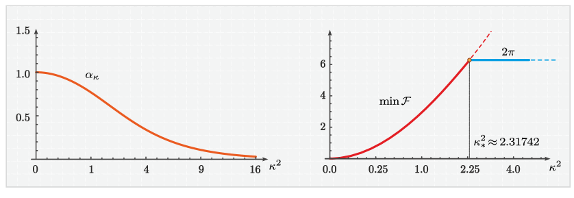
Figure 5. There is a critical value $\kappa_{\ast}^{2}$ of the anisotropy parameter, $\kappa_{\ast}^{2}\approx 2.31742$, below which the global minimizers of (4.1) have degree zero, and above which the only two global minimizers are the normal vector fields $\pm\boldsymbol{n}$ (and have degree one).

If $\boldsymbol{m}_{\bot}$ is a (global) minimizer in $H^{1}_{\sharp}([-\pi,\pi],\mathbb{S}^{1})$ of the energy functional $\mathcal{F}$ (cf. (4.1)), then either $\mathrm{deg\,}\boldsymbol{m}_{\bot}=0$ or $\mathrm{deg\,}\boldsymbol{m}_{\bot}=1$. Precisely, there exists a threshold value $\kappa^{2}_{\ast}$ of the anisotropy parameter such that the following dichotomy holds:

1. If $\kappa^{2}>\kappa_{\ast}^{2}$, then any global minimizer has degree one. Moreover, for every $\kappa^{2}>0$, the normal fields $\pm\boldsymbol{n}$ are the only two global minimizers of $\mathcal{F}$ in the homotopy class $\left\{\mathrm{deg\,}\boldsymbol{m}_{\bot}=1\right\}$.

2. If $\kappa^{2}<\kappa_{\ast}^{2}$, then any global minimizer has degree zero. Also, for any $\kappa^{2}>0$, the minimizers of $\mathcal{F}$ in the homotopy class $\left\{\mathrm{deg\,}\boldsymbol{m}_{\bot}\right\}=0$ are given by (cf. Figure 6)

   $$\boldsymbol{m}_{\bot}(t)=\sin\theta(t)\boldsymbol{\tau}(t)+\cos\theta(t)\boldsymbol{n}(t)$$ (4.7)

   with $\theta$ (a strictly decreasing function) being any element of the family

   $$\theta(t)=\operatorname{am}_{\kappa}(-\alpha_{\kappa}t+b),\quad b\in\mathbb{R}\,,$$ (4.8)

   and $\alpha_{\kappa}>0$ the unique solution of (4.3). Moreover, the minimal value of the energy is given by (cf. Figure 5)

   $$\mathcal{F}\left(\boldsymbol{m}_{\bot}\right)=-2\pi(1+\alpha_{\kappa}^{2})+2\alpha_{\kappa}E_{\kappa}.$$ (4.9)

3. The exact value of $\kappa^{2}_{\ast}$ is determined as the solution of the equation

   $$-2\pi\alpha_{\kappa}^{2}+2\alpha_{\kappa}E_{\kappa}=4\pi,$$ (4.10)

   which gives $\kappa^{2}_{\ast}\approx 2.31742$.

4. For any $\kappa^{2}>0$, the degree-zero solutions (4.8) are locally stable critical points of the energy $\mathcal{F}$ in (4.1). Also, for any $\kappa^{2}>0$, degree-one solutions $\pm\boldsymbol{n}$ are local minimizers of the energy $\mathcal{F}$.

Combining i and ii we get the following characterization of the energy landscape. The normal vector fields $\pm\boldsymbol{n}$ are the only two global minimizers of $\mathcal{F}$ when $\kappa^{2}>\kappa_{\ast}^{2}$ and the common minimum value of the energy is $2\pi$. When $\kappa^{2}<\kappa_{\ast}^{2}$ the minimal energy depends on $\kappa$, it is given by (4.9), and is reached when $\theta$ is given by (4.8). Finally, when $\kappa^{2}=\kappa_{\ast}^{2}$ both the degree one solutions $\pm\boldsymbol{n}$ and the degree zero solutions (4.7)-(4.8) coexist as energy minimizers and the common value of the energy is $2\pi$ (cf. Figure 5).

Remark 10.

Note that, while in the $\mathbb{S}^{1}$-valued setting the normal vector fields $\pm\boldsymbol{n}$ are local minimizers for every $\kappa^{2}>0$, this was not the case in the $\mathbb{S}^{2}$-valued setting reported in Theorem 3 (where $\pm\boldsymbol{n}$ become unstable for $\kappa^{2}<1$). The precise reason is that here we are restricted to the class of in-plane perturbations, whereas in the $\mathbb{S}^{2}$-valued case the loss of stability is caused by perturbations in the $\boldsymbol{e}_{3}$ direction.

Proof.

As in the proof of Theorem 2, it is convenient to set $\boldsymbol{m}_{\bot}=m_{1}\boldsymbol{\tau}+m_{2}\boldsymbol{n}$ with $m_{1}:=\boldsymbol{m}_{\bot}\cdot\boldsymbol{\tau}$ and $m_{2}:=\boldsymbol{m}_{\bot}\cdot\boldsymbol{n}$, where $\boldsymbol{n}(t)=(\cos t,\sin t,0)$ and $\boldsymbol{\tau}(t):=\partial_{t}\boldsymbol{n}(t)$ are the normal and tangential fields to $\mathbb{S}^{1}\times\{0\}$. Note that both $m_{1}$ and $m_{2}$ are in $H^{1}_{\sharp}([-\pi,\pi],\mathbb{R})$. In the moving frame $(\boldsymbol{\tau},\boldsymbol{n})$, the energy (4.1) assumes the expression (cf. (3.41))

$$\mathcal{F}(\boldsymbol{m}_{\bot})=\int_{-\pi}^{\pi}|\partial_{t}m_{2}-m_{1}|^{2}+|\partial_{t}m_{1}+m_{2}|^{2}\mathrm{d}t+\kappa^{2}\int_{-\pi}^{\pi}m_{1}^{2}\hskip 1.69998pt\mathrm{d}t.$$ (4.11)

Clearly, the vector field $(m_{1},m_{2})$ is $\mathbb{S}^{1}$-valued. We lift it by setting

$$m_{1}(t):=\sin\theta(t),\quad m_{2}(t):=\cos\theta(t).$$ (4.12)

After that, the energy (4.11) reads as

$$\mathcal{F}(\boldsymbol{m}_{\bot})=\; \int_{-\pi}^{\pi}|\partial_{t}\theta(t)+1|^{2}\mathrm{d}t+\kappa^{2}\int_{-\pi}^{\pi}\sin^{2}\theta(t)\mathrm{d}t$$ (4.13)

$$=\; \int_{-\pi}^{\pi}|\partial_{t}\theta(t)|^{2}+\kappa^{2}\sin^{2}\theta(t)\mathrm{d}t+2\pi+2(\theta(\pi)-\theta(-\pi)).$$ (4.14)

Figure 6. A plot of the vector fields minimizing the energy (4.1). There is a critical value $\kappa_{\ast}^{2}$ of the anisotropy parameter, $\kappa_{\ast}^{2}\approx 2.31742$, below which the global minimizers of (4.1) have degree zero, and above which the only two global minimizers are the normal vector fields $\pm\boldsymbol{n}$ (and have degree one). From left to right, we plot the minimizers for $\kappa^{2}=0.25$, $\kappa^{2}=1$, and $\kappa^{2}=2.25$.

It is clear that since $m_{1},m_{2}\in H^{1}_{\sharp}([-\pi,\pi],\mathbb{R})$ we necessarily have

$$\theta(\pi)-\theta(-\pi)=2\pi j$$ (4.15)

for some $j\in\mathbb{Z}$. Hence, the energy functional $\mathcal{F}$ takes the form

$$\mathcal{F}(\boldsymbol{m}_{\bot})=\int_{-\pi}^{\pi}|\partial_{t}\theta(t)|^{2}+\kappa^{2}\sin^{2}\theta(t)\mathrm{d}t+2\pi(1+2j)$$ (4.16)

The integer $j\in\mathbb{Z}$ is nothing but the degree of the $\mathbb{S}^{1}$-valued map $(m_{1},m_{2})$ whose components are the coordinates of $\boldsymbol{m}_{\bot}$ in the moving frame $(\boldsymbol{\tau},\boldsymbol{n})$. Therefore, from (4.15) we get that

$$\mathrm{deg\,}\boldsymbol{m}_{\bot}=j+1.$$ (4.17)

In fact, the previous relation can also be obtained from (4.15) observing that $\boldsymbol{m}_{\bot}=(\cos(\theta(t)+t),\sin(\theta(t)+t),0)$.

The expression (4.16) can be used to investigate the critical points of $\mathcal{F}$ in any prescribed homotopy class $j\in\mathbb{Z}$. Here, however, we are interested in global minimizers and, as we are going to show, this restricts the admissible homotopy classes to only two cases.

First, we use (4.15) and Jensen’s inequality for the Dirichlet part in (4.16) to get that

$$\mathcal{F}(\boldsymbol{m}_{\bot})\geqslant 2\pi(1+j)^{2}+\kappa^{2}\int_{-\pi}^{\pi}\sin^{2}\theta(t)\mathrm{d}t$$ (4.18)

for every $\boldsymbol{m}_{\bot}\in H^{1}_{\sharp}(\mathbb{S}^{1},\mathbb{S}^{1})$. Second, we recall that for every $\kappa^{2}>0$, we have $\mathcal{F}(\boldsymbol{n})=2\pi$, as well as $\mathcal{F}(\boldsymbol{\sigma})=\pi\kappa^{2}$ for any $\boldsymbol{\sigma}\in\mathbb{S}^{1}$. Therefore, if $\boldsymbol{m}_{\bot}$ is a minimizer of (4.16), then necessarily

$$2\pi(1+j)^{2}\leqslant\mathcal{F}(\boldsymbol{m}_{\bot})\leqslant\min\{2\pi,\pi\kappa^{2}\}.$$ (4.19)

Since $2\pi(1+j)^{2}>2\pi$ when $|1+j|>1$, from the previous bounds, we get that the global minimizers of $\mathcal{F}$ in $H^{1}_{\sharp}(\mathbb{S}^{1},\mathbb{S}^{1})$ have to satisfy the relation (4.15) with $j\in\{-2,-1,0\}$. On the other hand, if $j=-2$ we get that $\mathcal{F}(\boldsymbol{m}_{\bot})$ is strictly greater than $2\pi$ because the density $\kappa^{2}(\sin\theta)^{2}$ gives a positive contribution when $j\neq 0$. Hence, necessarily $j\in\{-1,0\}$. Hence, recalling (4.17),

$$\mathrm{deg\,}\boldsymbol{m}_{\bot}\in\{0,1\}.$$

This proves the first part of the statement.

Now, if $\boldsymbol{m}_{\bot}$ is a global minimizer of $\mathcal{F}$ and if $\mathrm{deg\,}\boldsymbol{m}_{\bot}=1$, i.e., if $j=0$, then from (4.19) we know that $2\pi\leqslant\mathcal{F}(\boldsymbol{m}_{\bot})\leqslant\pi\kappa^{2}$. Hence, necessarily $\kappa^{2}\geqslant 2$ if $\mathrm{deg\,}\boldsymbol{m}_{\bot}=1$. It follows that $\mathrm{deg\,}\boldsymbol{m}_{\bot}=0$ whenever $\kappa^{2}<2$. Also, if $\kappa^{2}\geqslant 3$, then Theorem 3 implies that $\pm\boldsymbol{n}$ are the only two global minimizers of $\mathcal{F}$, and these belong to the homotopy class $\mathrm{deg\,}\boldsymbol{m}_{\bot}=1$. Therefore, if $\kappa^{2}\geqslant 3$, then any global minimizer has degree one, and if $\kappa^{2}<2$, then any global minimizer has degree zero.

Note that, at this stage, we cannot infer the existence of a threshold $\kappa_{\ast}^{2}\in[2,3]$ such that any global minimizer has degree one when $\kappa^{2}>\kappa_{\ast}^{2}$, and any global minimizer has degree zero when $\kappa^{2}<\kappa_{\ast}^{2}$. Indeed, in principle, it can still be the case that the minimizing homotopy classes are not described by intervals. However, from the characterization of the minimizer in the homotopy classes $\mathrm{deg\,}\boldsymbol{m}_{\bot}=0$ (given in the proof of ii.) and from the comparison of the associated energies (given in the proof of iii.), it immediately follows that there exists a unique $\kappa^{2}_{\ast}$

$$\kappa^{2}_{\ast}\in[2,3]$$ (4.20)

such that if $\kappa^{2}>\kappa_{\ast}^{2}$, then any global minimizer has degree one, and if $\kappa^{2}<\kappa_{\ast}^{2}$, then any global minimizer has degree zero.

Proof of i. It remains to show that for every $\kappa>0$, the vector fields $\pm\boldsymbol{n}$ are the only two global minimizers of $\mathcal{F}$ in the homotopy class $\mathrm{deg\,}\boldsymbol{m}_{\bot}=1$. For that, it is sufficient to observe that when $j=0$, from (4.18), we get that $\mathcal{F}(\boldsymbol{m}_{\bot})\geqslant 2\pi=\mathcal{F}(\pm\boldsymbol{n})$ regardless of the value of $\kappa^{2}>0$. Moreover, $\mathcal{F}(\boldsymbol{m}_{\bot})>2\pi$ if $\|\sin\theta\|^{2}_{L^{2}[-\pi,\pi]}\neq 0$, i.e., if $\boldsymbol{m}_{\bot}\notin\{\pm\boldsymbol{n}\}$. This guarantees the uniqueness statement about the minimizers $\pm\boldsymbol{n}$.

Proof of ii. We want to improve the estimate (4.20), but we also want to identify the minimizers of $\mathcal{F}$ in the prescribed homotopy class $\mathrm{deg\,}\boldsymbol{m}_{\bot}=0$. This amounts to the minimization problem for $\mathcal{F}$ under the constraint $j=-1$ in (4.15). In other words, one has to minimize energy (cf. (4.16))

$$\mathcal{F}(\boldsymbol{m}_{\bot})=-2\pi+\int_{-\pi}^{\pi}|\partial_{t}\theta(t)|^{2}+\kappa^{2}\sin^{2}\theta(t)\mathrm{d}t$$ (4.21)

under the constraint that $\theta(\pi)-\theta(-\pi)=-2\pi$ (cf. (4.15)). The Euler–Lagrange equations associated with (4.21) gives the equation

$$\partial_{tt}\theta(t)=\kappa^{2}\sin\theta(t)\cos\theta(t),$$ (4.22)

subject to the degree constraint

$$\theta(\pi)=\theta(-\pi)-2\pi.$$ (4.23)

It is worth noticing that, from the mechanical point of view, the nonlinear ordinary differential equation (4.22) describes the dynamics of an (ideal) inverted pendulum in the reduced setting where the pivot point of the pendulum is fixed in space (cf. Figure 7). In this reduced setting, the equation of the inverted pendulum, up to a sign, is the one of a simple pendulum (see, e.g., [6, p. 35]), the difference being in the nominal location of the pivot point which, for the inverted pendulum, is below its center of mass. Precisely, if the inverted pendulum consists of a spherical mass subject to the force of gravity $g$, placed at the end of a rigid massless rod of length $\ell$ then, its equation is given by (4.22) with $\kappa^{2}=g/\ell$. Using this mechanical analogy, the minimizers $\boldsymbol{m}_{\bot}$ in the class $\left\{\mathrm{deg\,}\boldsymbol{m}_{\bot}=0\right\}$ we are interested in, correspond to solutions of the inverted pendulum in which the mass $m$ performs a full clockwise turn at the minimal cost of the energy (4.21).

Figure 7. (Left) The ideal inverted pendulum consists of a spherical mass $m$, subject to the force of gravity $g$, placed at the end of a rigid massless rod of length $\ell$ attached to a (possibly oscillating) pivot point. When the pivot point of the pendulum is fixed in space, the equation of motion, up to a sign, is the one of a simple pendulum; the difference is in the nominal location of the pivot point which, for the inverted pendulum, is below its center of mass. (Right) The typical phase portrait of the inverted pendulum (4.22). It consists of the level sets of the function $f_{\kappa}(x,y):=y^{2}-\kappa^{2}\sin^{2}x$. The maximal quote of the separatrix $\Sigma:=f_{\kappa}^{-1}(0)$ is achieved at $|\kappa|$; here $\kappa^{2}=1.5$. The closed level curves correspond to oscillations of the pendulum about its equilibrium position $2\theta=\pm\pi$, while the curves outside the separatrix $\Sigma$ correspond to full rotations of the pendulum.

The problem is solvable in terms of elliptic integrals. For that, we observe that by multiplying both parts of (4.23) by $\partial_{t}{\theta}$ one gets that if the integral curve

$$t\in[-\pi,\pi]\mapsto(\theta(t),\partial_{t}\theta(t))\in\mathbb{R}^{2}$$ (4.24)

solves (4.23) then there exists a constant $c_{\kappa}\in\mathbb{R}$ such that

$$(\partial_{t}\theta(t))^{2}-\kappa^{2}\sin^{2}\theta(t)=c_{\kappa}\quad\forall t\in[-\pi,\pi].$$ (4.25)

Precisely, $c_{\kappa}:=|\partial_{t}\theta(-\pi)|^{2}-\kappa^{2}\sin^{2}\theta(-\pi)$. In other words, every solution $(\theta(t),\partial_{t}\theta(t))$ of the boundary value problem (4.23) belongs to some level set of the function $f_{\kappa}(x,y):=y^{2}-\kappa^{2}\sin^{2}x$, with the understanding that we formally set $y:=\partial_{t}\theta$ and $x:=\theta$. The phase diagram is depicted in Figure 7 where the thicker line represents the separatrix

$$\Sigma:=\left\{(x,y)\in\mathbb{R}^{2}:y^{2}=\kappa^{2}\sin^{2}x\right\}$$ (4.26)

which bounds the region

$$S:=\left\{(x,y)\in\mathbb{R}^{2}:y^{2}\leqslant\kappa^{2}\sin^{2}x\right\}.$$ (4.27)

Note that the phase diagram is periodic (in the $x$-direction) of period $\pi$. However, it is convenient to consider the range $-\pi\leqslant x=\theta\leqslant\pi$ of length $2\pi$ because we are interested in solutions such that $\theta(\pi)-\theta(-\pi)=-2\pi$. From the phase diagram represented in Figure 7, it is clear that the solutions we are interested in are such that the coordinate $y=\partial_{t}\theta$ never vanishes, as this is the only way to connect, via a phase curve, two points of the phase portrait whose $x$ coordinates are $2\pi$ away. The rigorous proof follows by observing that the region $S$ includes the level sets $\{f_{\kappa}^{-1}(c)\}_{c<0}$ which consist of disjoint compact subsets of $S$, each one of them projecting on the $x$-axis on a set of diameter less than $\pi$. However, the solution curves $\alpha(t):=(\theta(t),\partial_{t}\theta(t))$ we are interested in, have to satisfy (4.23) and, therefore, must have a trace in the phase space whose projection on the $x$-axis has diameter $2\pi$. It follows that any solution $\alpha(t):=(\theta(t),\partial_{t}\theta(t))$ of (4.22)-(4.23) lies on the level set $f_{\kappa}^{-1}(c_{\kappa})$ for some $c_{\kappa}\geqslant 0$. After that, we observe that the solutions lying on the level set $f_{\kappa}^{-1}(0)$ whose projection on the $x$-axis have diameter $2\pi$ correspond to the normal vector fields $\pm\boldsymbol{n}$; hence, from now on, we focus on solutions in $S^{\complement}=\cup_{c>0}f^{-1}(c)$. Given the expression of $c_{\kappa}$, this implies that

$$|\partial_{t}\theta(-\pi)|^{2}>\kappa^{2}\sin^{2}\theta(-\pi).$$ (4.28)

First, we note that if $(x,y)\in S^{\complement}$ then $y\neq 0$. Therefore, the solutions of (4.22)-(4.23) are such that $\partial_{t}\theta(t)\neq 0$ for every $t\in[-\pi,\pi]$. Thus, $\theta$ is either decreasing or increasing. But given the degree condition (4.23) the solutions we are looking for have to be decreasing. Therefore, from (4.25), we get that

$$\partial_{t}\theta(t)=-\sqrt{|\partial_{t}\theta(-\pi)|^{2}-\kappa^{2}\sin^{2}\theta(-\pi)+\kappa^{2}\sin^{2}\theta(t)}.$$ (4.29)

It is convenient to set

$$\alpha_{\kappa}:=\sqrt{|\partial_{t}\theta(-\pi)|^{2}-\kappa^{2}\sin^{2}\theta(-\pi)},$$ (4.30)

because, as we are going to show, the value of $\alpha_{\kappa}$ just defined coincides with the value defined by (4.3). Note that $\alpha_{\kappa}>0$ due to (4.28). The expression of $\partial_{t}\theta(t)$ can be rewritten under the form

$$\partial_{t}\theta(t)=-\alpha_{\kappa}\sqrt{1+(\kappa^{2}/\alpha^{2}_{\kappa})\sin^{2}\theta(t)}.$$ (4.31)

Next, we observe that the elliptic integral of the first kind $F_{\kappa}$ (defined in (4.5)) is increasing (invertible) and vanishes at $-\pi$. Therefore from (4.31) we deduce that

$$F_{\kappa}(\theta(t))-F_{\kappa}(\theta(-\pi))=-(t+\pi)\alpha_{\kappa}.$$ (4.32)

In particular, evaluating the previous relation at $t=\pi$ and taking into account (4.23) we obtain

$$F_{\kappa}(\theta(\pi))-F_{\kappa}(\theta(-\pi))=-2\pi\alpha_{\kappa}.$$ (4.33)

On the other hand, the integrand defining $F_{\kappa}$ is periodic of period $\pi$ and, therefore, taking also into account that $\theta(\pi)=\theta(-\pi)-2\pi$, we obtain

$$F_{\kappa}(\theta(\pi))-F_{\kappa}(\theta(-\pi))=\; \int_{\theta(-\pi)}^{\theta(-\pi)-2\pi}\frac{1}{\sqrt{1+(\kappa^{2}/\alpha^{2}_{\kappa})\sin^{2}x}}\mathrm{d}x$$

$$=\; -\int_{-\pi}^{\pi}\frac{1}{\sqrt{1+(\kappa^{2}/\alpha^{2}_{\kappa})\sin^{2}x}}\mathrm{d}x$$

$$=\; -2\pi\beta_{\kappa},$$ (4.34)

where we set $\beta_{\kappa}:=1/(2\pi)F_{\kappa}(\pi)$. From (4.33) and (4.34) it follows that if $(\theta(t),\partial_{t}\theta(t))$ is a solution of our problem (4.22)-(4.23) then necessarily $\alpha_{\kappa}=\beta_{\kappa}$. Therefore the value of $\alpha_{\kappa}$ can be characterized as the unique solution of the equation (cf. (4.3))

$$\frac{1}{2\pi}\int_{-\pi}^{\pi}\frac{1}{\sqrt{\alpha^{2}_{\kappa}+\kappa^{2}\sin^{2}x}}\mathrm{d}x=1.$$ (4.35)

Once computed $\alpha_{\kappa}$, we can characterize the solutions of (4.22)-(4.23) using (4.33), which gives the one-parameter family of functions $\theta(t)=F^{-1}_{\kappa}\left(F_{\kappa}(\theta(-\pi))-(t+\pi)\alpha_{\kappa}\right)$, $\theta(-\pi)\in\mathbb{R}$, which, by the way, is of the form

$$\theta(t)=\operatorname{am}_{\kappa}(-\alpha_{\kappa}t+b_{\kappa}),\qquad b_{\kappa}:=F_{\kappa}(\theta(-\pi))-\pi\alpha_{\kappa}\in\mathbb{R}.$$ (4.36)

This proves (4.8) and gives a parameterization of the family of solutions in terms of the initial condition $\theta(-\pi)$, or in terms of the initial condition $\partial_{t}\theta(-\pi)$ due to (4.30).

In principle, the energy can depend on $b_{\kappa}$, but this is not the case as we are going to show next. For that, we observe that from (4.31) we get that

$$|\partial_{t}\theta(t)|^{2}=\alpha_{\kappa}^{2}+\kappa^{2}\sin^{2}\theta(t).$$ (4.37)

Plugging the previous expression into the energy functional (4.21), we obtain that if $\boldsymbol{m}_{\bot}$ minimizes the energy in the homotopy class $\left\{\mathrm{deg\,}\boldsymbol{m}_{\bot}=0\right\}$, then

$$\mathcal{F}(\boldsymbol{m}_{\bot})=-2\pi(1+\alpha_{\kappa}^{2})+2\int_{-\pi}^{\pi}|\partial_{t}\theta(t)|^{2}\mathrm{d}t.$$ (4.38)

Next, we observe that since $\theta$ is a decreasing function, we have that

$$\int_{-\pi}^{\pi}|\partial_{t}\theta(t)|^{2}\mathrm{d}t=\; \int_{\theta(\pi)}^{\theta(-\pi)}|(\partial_{t}\theta\circ\theta^{-1})(x)|^{2}|\partial_{x}\theta^{-1}(x)|\mathrm{d}x$$

$$=\; \int_{\theta(\pi)}^{\theta(-\pi)}\frac{1}{|\partial_{x}\theta^{-1}(x)|}\mathrm{d}x.$$ (4.39)

But from (4.36) we know that $\theta^{-1}(x)=\frac{b_{\kappa}-F_{\kappa}(x)}{\alpha_{\kappa}}$ and, therefore

$$\int_{-\pi}^{\pi}|\partial_{t}\theta(t)|^{2}\mathrm{d}t=\; \alpha_{\kappa}\int_{\theta(\pi)}^{\theta(-\pi)}\frac{1}{|F^{\prime}_{\kappa}(x)|}\mathrm{d}x$$

$$=\; \alpha_{\kappa}\int_{\theta(\pi)}^{\theta(-\pi)}\sqrt{1+(\kappa^{2}/\alpha^{2}_{\kappa})\sin^{2}x}\,\mathrm{d}x.$$ (4.40)

Making use of the $\pi$-periodicity of the integrand, from (4.6) and (4.23) we infer that

$$\int_{-\pi}^{\pi}|\partial_{t}\theta(t)|^{2}\mathrm{d}t=\alpha_{\kappa}\int_{-\pi}^{\pi}\sqrt{1+(\kappa^{2}/\alpha^{2}_{\kappa})\sin^{2}x}\,\mathrm{d}x=\alpha_{\kappa}E_{\kappa}.$$ (4.41)

Overall, plugging the previous expression into the expression (4.38) of the energy, we get

$$\mathcal{F}(\boldsymbol{m}_{\bot})=-2\pi(1+\alpha_{\kappa}^{2})+2\alpha_{\kappa}E_{\kappa}$$ (4.42)

and this proves (4.9).

Proof of iii. The proof quickly follows from i and ii because the energy of the normal vector fields $\pm\boldsymbol{n}$ evaluates to $2\pi$ and, therefore, due to (4.42), degree zero configurations given by (4.36) are preferred as soon as

$$-2\pi(1+\alpha_{\kappa}^{2})+2\alpha_{\kappa}E_{\kappa}<2\pi.$$ (4.43)

This happens when $\kappa^{2}<\kappa^{2}_{\ast}\approx 2.31742$.

Proof of iv. Finally, we want to show that the degree zero solutions (4.36), which we know to be global minimizers when $\kappa^{2}<\kappa^{2}_{\ast}$, retain local stability for every $\kappa^{2}>0$. For that, we compute the second variation of the energy (4.11) which, for any $\phi\in H^{1}_{\sharp}([-\pi,\pi],\mathbb{R})$, reads as (cf. (4.13))

$$\mathcal{F}^{\prime\prime}(\theta)(\phi)=\int_{-\pi}^{\pi}|\partial_{t}\phi(t)|^{2}+\kappa^{2}\phi^{2}(t)\cos 2\theta(t)\hskip 1.69998pt\mathrm{d}t.$$ (4.44)

From the Euler-Lagrange equations (4.22) we get that

$$\partial_{ttt}\theta=\kappa^{2}(\cos 2\theta)\partial_{t}\theta.$$ (4.45)

Moreover, since $|\partial_{t}\theta|\geqslant c^{\prime}_{\theta}>0$ on the compact set $[-\pi,\pi]$ for some $c_{\theta}>0$, we can use the Hardy decomposition trick (see [12, 26, 27, 28, 29]) and say that any $\phi\in H^{1}_{\sharp}([-\pi,\pi],\mathbb{R})$ can be written as $\phi=(\partial_{t}\theta)\psi$ for some $\psi\in H^{1}_{\sharp}([-\pi,\pi],\mathbb{R})$. Therefore

$$\mathcal{F}^{\prime\prime}(\theta)(\phi)=\int_{-\pi}^{\pi}|\partial_{t}\theta|^{2}|\partial_{t}\psi|^{2}+|\partial_{tt}\theta|^{2}|\psi|^{2}+\partial_{tt}\theta\partial_{t}\theta\partial_{t}\left|{\psi^{2}}\right|+\kappa^{2}|\psi|^{2}|\partial_{t}\theta|^{2}(\cos 2\theta)\hskip 1.69998pt\mathrm{d}t.$$ (4.46)

Integrating by parts the previous expression and making use of (4.45) we obtain

$$\mathcal{F}^{\prime\prime}(\theta)(\phi)\,=\,\int_{-\pi}^{\pi}|\partial_{t}\theta|^{2}|\partial_{t}\psi|^{2}\hskip 1.69998pt\mathrm{d}t\,\geqslant\,(c^{\prime}_{\theta})^{2}\int_{-\pi}^{\pi}|\partial_{t}\psi|^{2}\hskip 1.69998pt\mathrm{d}t.$$ (4.47)

Finally, plugging $\theta=0$ into (4.44), we get that $\pm\boldsymbol{n}$ are uniform locally stable critical points for every $\kappa^{2}>0$. Therefore, since the lifting (4.12) preserves small $H^{1}$ neighborhoods, we get that $\pm\boldsymbol{n}$ are local minimizers of the energy $\mathcal{F}$. This concludes the proof. ∎

5. Acknowledgments

G. Di F. acknowledges support from the Austrian Science Fund (FWF) through the special research program Taming complexity in partial differential systems (Grant SFB F65) and the project Analysis and Modeling of Magnetic Skyrmions (grant P-34609). G. Di F. also thanks TU Wien and MedUni Wien for their support and hospitality.

The work of the V. S. was supported by the EPSRC grant EP/K02390X/1 and the Leverhulme grant RPG-2018-438. G. Di F. and V. S. would like to thank the Max Planck Institute for Mathematics in the Sciences in Leipzig for support and hospitality. G. Di F., A. F., and V. S. acknowledge support from ESI, the Erwin Schrödinger International Institute for Mathematics and Physics in Wien, given in occasion of the Workshop on New Trends in the Variational Modeling and Simulation of Liquid Crystals held at ESI, in Wien, on December 2-6, 2019.

Giovanni Di Fratta, Dipartimento di Matematica e Applicazioni “R. Caccioppoli”, Università degli Studi di Napoli “Federico II”, Via Cintia, Complesso Monte S. Angelo, 80126 Napoli, Italy. E-mail address: giovanni.difratta@unina.it

Alberto Fiorenza, Dipartimento di Architettura, Università di Napoli Federico II, Via Monteoliveto, 3, I-80134 Napoli, Italy, and Istituto per le Applicazioni del Calcolo “Mauro Picone”, sezione di Napoli, Consiglio Nazionale delle Ricerche, via Pietro Castellino, 111, I-80131 Napoli, Italy. E-mail address: fiorenza@unina.it

Valeriy Slastikov, School of Mathematics, University of Bristol, University Walk, Bristol BS8 1TW, United Kingdom. E-mail address: valeriy.slastikov@bristol.ac.uk

References

- [1] M. S. Agranovich, Sobolev Spaces, Their Generalizations and Elliptic Problems in Smooth and Lipschitz Domains, Springer International Publishing, 2015.
- [2] F. Alouges, A new algorithm for computing liquid crystal stable configurations: the harmonic mapping case, SIAM Journal on Numerical Analysis, 34 (1997), pp. 1708–1726.
- [3] F. Alouges, A new finite element scheme for Landau-Lifchitz equations, Discrete & Continuous Dynamical Systems - S, 1 (2008), pp. 187–196.
- [4] F. Alouges, G. Di Fratta, and B. Merlet, Liouville type results for local minimizers of the micromagnetic energy, Calculus of Variations and Partial Differential Equations, 53 (2015), pp. 525–560.
- [5] F. Alouges and A. Soyeur, On global weak solutions for Landau-Lifshitz equations: Existence and nonuniqueness, Nonlinear Analysis: Theory, Methods & Applications, 18 (1992), pp. 1071–1084.
- [6] H. Amann, Ordinary differential equations: an introduction to nonlinear analysis, vol. 13, Walter de Gruyter, 2011.
- [7] J.-F. Babadjian, G. Di Fratta, I. Fonseca, G. A. Francfort, M. Lewicka, and C. B. Muratov, The mathematics of thin structures, Quarterly of Applied Mathematics, Published electronically: September 1, 2022 .
- [8] W. F. Brown, The Fundamental Theorem of the Theory of Fine Ferromagnetic Particles, Annals of the New York Academy of Sciences, 147 (1969), pp. 463–488.
- [9] G. Carbou, Thin Layers in Micromagnetism, Mathematical Models and Methods in Applied Sciences, 11 (2002), pp. 1529–1546.
- [10] E. Davoli and G. Di Fratta, Homogenization of Chiral Magnetic Materials: A Mathematical Evidence of Dzyaloshinskii’s Predictions on Helical Structures, Journal of Nonlinear Science, (2020).
- [11] E. Davoli, G. Di Fratta, D. Praetorius, and M. Ruggeri, Micromagnetics of thin films in the presence of Dzyaloshinskii–Moriya interaction, Mathematical Models and Methods in Applied Sciences, 32.5 (2022), pp. 911–939,
- [12] G. Di Fratta, J. M. Robbins, V. Slastikov, and A. D. Zarnescu, Half-integer point defects in the -tensor theory of nematic liquid crystals, Journal of Nonlinear Science, 26 (2015), pp. 121–140.
- [13] G. Di Fratta, C. Serpico, and M. dAquino, A generalization of the fundamental theorem of Brown for fine ferromagnetic particles, Physica B: Condensed Matter, 407 (2012), pp. 1368–1371.
- [14] G. Di Fratta, Micromagnetics of curved thin films, Zeitschrift für angewandte Mathematik und Physik, 71 (2020).
- [15] G. Di Fratta, M. Innerberger, and D. Praetorius, Weak-strong uniqueness for the Landau–Lifshitz–Gilbert equation in micromagnetics, Nonlinear Analysis: Real World Applications, 55 (2020), p. 103122.
- [16] G. Di Fratta, M. Innerberger, D. Praetorius, and V. Slastikov, An energy minimization scheme for the analysis of magnetic skyrmions in thin films, In preparation, (2021).
- [17] G. Di Fratta, C. B. Muratov, F. N. Rybakov, and V. V. Slastikov, Variational principles of micromagnetics revisited, SIAM Journal on Mathematical Analysis, 52 (2020), pp. 3580–3599.
- [18] G. Di Fratta, C.-M. Pfeiler, D. Praetorius, M. Ruggeri, and B. Stiftner, Linear second-order IMEX-type integrator for the (eddy current) Landau–Lifshitz–Gilbert equation, IMA Journal of Numerical Analysis, 40 (2019), pp. 2802–2838.
- [19] G. Di Fratta, V. Slastikov, and A. Zarnescu, On a sharp Poincaré-type inequality on the 2-sphere and its application in micromagnetics, SIAM Journal on Mathematical Analysis, 51 (2019), pp. 3373–3387.
- [20] G. Di Fratta, A. Monteil, and V. Slastikov, Symmetry properties of minimizers of a perturbed Dirichlet energy with a boundary penalization, SIAM Journal on Mathematical Analysis, 54.3 (2022), pp. 3636–3653.
- [21] A. Fiorenza, M. R. Formica, T. Roskovec, and F. Soudský, Detailed proof of classical Gagliardo-Nirenberg interpolation inequality with historical remarks, To appear in Zeitschrift für Analysis und ihre Anwendungen, (2021).
- [22] Y. Gaididei, V. P. Kravchuk, and D. D. Sheka, Curvature effects in thin magnetic shells, Physical Review Letters, 112 (2014), p. 257203.
- [23] G. Gioia and R. D. James, Micromagnetics of very thin films, Proceedings of the Royal Society A: Mathematical, Physical and Engineering Sciences, 453 (1997), pp. 213–223.
- [24] S.-H. Hu, S.-Y. Chen, D.-M. Liu, and C.-S. Hsiao, Core/Single-Crystal-Shell Nanospheres for Controlled Drug Release via a Magnetically Triggered Rupturing Mechanism, Advanced Materials, 20 (2008), pp. 2690–2695.
- [25] R. Ignat and R. L. Jerrard, Renormalized energy between vortices in some Ginzburg–Landau models on 2-dimensional Riemannian manifolds, Archive for Rational Mechanics and Analysis, 239 (2021), pp. 1577–1666.
- [26] R. Ignat, L. Nguyen, V. Slastikov, and A. Zarnescu, Stability of the melting hedgehog in the Landau–de Gennes theory of nematic liquid crystals, Archive for Rational Mechanics and Analysis, 215 (2015), pp. 633–673.
- [27] R. Ignat, L. Nguyen, V. Slastikov, and A. Zarnescu, Instability of point defects in a two-dimensional nematic liquid crystal model, Annales de l’Institut Henri Poincaré. Analyse Non Linéaire, 33 (2016), pp. 1131–1152.
- [28] R. Ignat, L. Nguyen, V. Slastikov, and A. Zarnescu, Stability of point defects of degree in a two-dimensional nematic liquid crystal model, Calculus of Variations and Partial Differential Equations, 55 (2016). Art. 119, 33.
- [29] R. Ignat, L. Nguyen, V. Slastikov, and A. Zarnescu, On the uniqueness of minimisers of Ginzburg-Landau functionals, Annales Scientifiques de l’École Normale Supérieure. Quatrième Série, 53 (2020), pp. 589–613.
- [30] V. P. Kravchuk, D. D. Sheka, R. Streubel, D. Makarov, O. G. Schmidt, and Y. Gaididei, Out-of-surface vortices in spherical shells, Physical Review B - Condensed Matter and Materials Physics, 85 (2012), pp. 1–6.
- [31] C. Melcher and Z. N. Sakellaris, Curvature-stabilized skyrmions with angular momentum, Letters in Mathematical Physics, 109 (2019), pp. 2291–2304.
- [32] D. S. Miller, X. Wang, and N. L. Abbott, Design of functional materials based on liquid crystalline droplets, Chemistry of Materials, 26 (2013), pp. 496–506.
- [33] J. Milnor, Topology from the differentiable viewpoint, Princeton Landmarks in Mathematics and Physics, Princeton University Press, 1997.
- [34] R. Moser, Partial regularity for harmonic maps and related problems, World Scientific Publishing Co. Pte. Ltd., Hackensack, NJ, 2005.
- [35] C. B. Muratov and V. V. Slastikov, Domain structure of ultrathin ferromagnetic elements in the presence of Dzyaloshinskii-Moriya Interaction, Proceedings of the Royal Society A: Mathematical, Physical and Engineering Sciences, 473 (2017), p. 20160666.
- [36] G. Napoli and L. Vergori, Extrinsic curvature effects on nematic shells, Physical Review Letters, 108 (2012), p. 207803.
- [37] O. G. Schmidt and K. Eberl, Thin solid films roll up into nanotubes, Nature, 410 (2001), pp. 168–168.
- [38] R. Schoen and K. Uhlenbeck, Boundary regularity and the Dirichlet problem for harmonic maps, Journal of Differential Geometry, 18.2 (1983), pp. 253–268.
- [39] F. Serra, Curvature and defects in nematic liquid crystals, Liquid Crystals, 43.13-15, pp. 1920-1936.
- [40] D. D. Sheka, D. Makarov, H. Fangohr, O. M. Volkov, H. Fuchs, J. van den Brink, Y. Gaididei, U. K. Rößler, and V. P. Kravchuk, Topologically stable magnetization states on a spherical shell: Curvature-stabilized skyrmions, Physical Review B, 94 (2016), pp. 1–10.
- [41] V. Slastikov, Micromagnetics of Thin Shells, Mathematical Models and Methods in Applied Sciences, 15 (2005), pp. 1469–1487.
- [42] V. V. Slastikov and C. Sonnenberg, Reduced models for ferromagnetic nanowires, IMA Journal of Applied Mathematics (Institute of Mathematics and Its Applications), 77 (2012), pp. 220–235.
- [43] M. I. Sloika, D. D. Sheka, V. P. Kravchuk, O. V. Pylypovskyi, and Y. Gaididei, Geometry induced phase transitions in magnetic spherical shell, Journal of Magnetism and Magnetic Materials, 443 (2017), pp. 404–412.
- [44] R. Streubel, P. Fischer, F. Kronast, V. P. Kravchuk, D. D. Sheka, Y. Gaididei, O. G. Schmidt, and D. Makarov, Magnetism in curved geometries, Journal of Physics D: Applied Physics, 49 (2016), p. 363001.