[table]capposition=top \newfloatcommandcapbtabboxtable[][]
LoveDA: A Remote Sensing Land-Cover Dataset for Domain Adaptive Semantic Segmentation
Abstract
Deep learning approaches have shown promising results in remote sensing high spatial resolution (HSR) land-cover mapping. However, urban and rural scenes can show completely different geographical landscapes, and the inadequate generalizability of these algorithms hinders city-level or national-level mapping. Most of the existing HSR land-cover datasets mainly promote the research of learning semantic representation, thereby ignoring the model transferability. In this paper, we introduce the Land-cOVEr Domain Adaptive semantic segmentation (LoveDA) dataset to advance semantic and transferable learning. The LoveDA dataset contains 5987 HSR images with 166768 annotated objects from three different cities. Compared to the existing datasets, the LoveDA dataset encompasses two domains (urban and rural), which brings considerable challenges due to the: 1) multi-scale objects; 2) complex background samples; and 3) inconsistent class distributions. The LoveDA dataset is suitable for both land-cover semantic segmentation and unsupervised domain adaptation (UDA) tasks. Accordingly, we benchmarked the LoveDA dataset on eleven semantic segmentation methods and eight UDA methods. Some exploratory studies including multi-scale architectures and strategies, additional background supervision, and pseudo-label analysis were also carried out to address these challenges. The code and data are available at https://github.com/Junjue-Wang/LoveDA.
1 Introduction
With the continuous development of society and economy, the human living environment is gradually being differentiated, and can be divided into urban and rural zones [8]. High spatial resolution (HSR) remote sensing technology can help us to better understand the geographical and ecological environment. Specifically, land-cover semantic segmentation in remote sensing is aimed at determining the land-cover type at every image pixel. The existing HSR land-cover datasets such as the Gaofen Image Dataset (GID) [38], DeepGlobe [9], Zeebruges [24], and Zurich Summer [43] contain large-scale images with pixel-wise annotations, thus promoting the development of fully convolutional networks (FCNs) in the field of remote sensing [46, 49]. However, these datasets are designed only for semantic segmentation, and they ignore the diverse styles among geographic areas. For urban and rural areas, in particular, the manifestation of the land cover is completely different, in the class distributions, object scales, and pixel spectra. In order to improve the model generalizability for large-scale land-cover mapping, appropriate datasets are required.
In this paper, we introduce an HSR dataset for Land-cOVEr Domain Adaptive semantic segmentation (LoveDA) for use in two challenging tasks: semantic segmentation and UDA. Compared with the UDA datasets [22, 39] that use simulated images, the LoveDA dataset contains real urban and rural remote sensing images. Exploring the use of deep transfer learning methods on this dataset will be a meaningful way to promote large-scale land-cover mapping. The major characteristics of this dataset are summarized as follows: 1) Multi-scale objects. The HSR images were collected from 18 complex urban and rural scenes, covering three different cities in China. The objects in the same category are in completely different geographical landscapes in the different scenes, which increases the scale variation. 2) Complex background samples. The remote sensing semantic segmentation task is always faced with the complex background samples (i.e., land-cover objects that are not of interest) [29, 54], which is particularly the case in the LoveDA dataset. The high-resolution and different complex scenes bring more rich details as well as larger intra-class variance for the background samples. 3) Inconsistent class distributions. The urban and rural scenes have different class distributions. The urban scenes with high population densities contain lots of artificial objects such as buildings and roads. In contrast, the rural scenes include more natural elements, such as forest and water. Compared with UDA datasets [42, 30] in general computer vision, the LoveDA dataset focuses on the style differences of the geographical environments. The inconsistent class distributions pose a special challenge for the UDA task.
As the LoveDA dataset was built with two tasks in mind, both advanced semantic segmentation and UDA methods were evaluated. Several exploratory experiments were also conducted to solve the particular challenges inherent in this dataset, and to inspire further research. A stronger representational architecture and UDA method are needed to jointly promote large-scale land cover mapping.
2 Related Work
| Image level | Resolution (m) | Dataset | Year | Sensor | Area () | Classes | Image width | Images | Task | |
| SS | UDA | |||||||||
| Meter level | 10 | LandCoverNet [1] | 2020 | Sentinel-2 | 30000 | 7 | 256 | 1980 | ||
| 4 | GID [38] | 2020 | GF-2 | 75900 | 5 | 48006300 | 150 | |||
| Sub-meter level | 0.250.5 | LandCover.ai [2] | 2020 | Airborne | 216.27 | 3 | 42009500 | 41 | ||
| 0.6 | Zurich Summer [43] | 2015 | QuickBird | 9.37 | 8 | 6221830 | 20 | |||
| 0.5 | DeepGlobe [9] | 2018 | WorldView-2 | 1716.9 | 7 | 2448 | 1146 | |||
| 0.05 | Zeebruges [24] | 2018 | Airborne | 1.75 | 8 | 10000 | 7 | |||
| 0.05 | ISPRS Potsdam 1 | 2013 | Airborne | 3.42 | 6 | 6000 | 38 | |||
| 0.09 | ISPRS Vaihingen 2 | 2013 | Airborne | 1.38 | 6 | 18873816 | 33 | |||
| 0.07 | AIRS [6] | 2019 | Airborne | 475 | 2 | 10000 | 1047 | |||
| 0.5 | SpaceNet [41] | 2017 | WorldView-2 | 2544 | 2 | 406439 | 6000 | |||
| 0.3 | LoveDA (Ours) | 2021 | Spaceborne | 536.15 | 7 | 1024 | 5987 | |||
-
The abbreviations are: SS – semantic segmentation, UDA – unsupervised domain adaptation.
2.1 Land-cover semantic segmentation datasets
Land-cover semantic segmentation, as a long-standing research topic, has been widely explored over the past decades. The early research relied on low- and medium-resolution datasets, such as MCD12Q1 [33], the National Land Cover Database (NLCD) [14], GlobeLand30 [15], LandCoverNet [1], etc. However, these studies all focused on large-scale mapping and analysis from a macro-level. With the advancement of remote sensing technology, massive HSR images are now being obtained on a daily basis from both spaceborne and airborne platforms. Due to the advantages of the clear geometrical structure and fine texture, HSR land-cover datasets are tailored for specific scenes at a micro-level. As is shown in Table 1, datasets such as ISPRS Potsdam 111http://www2.isprs.org/commissions/comm3/wg4/2d-sem-label-potsdam.html , ISPRS Vaihingen 222http://www2.isprs.org/commissions/comm3/wg4/2d-sem-label-vaihingen.html , Zurich Summer [43], and Zeebruges [24] are designed for urban parsing. These datasets only contain a small number of annotated images and cover limited areas. In contrast, DeepGlobe [9] and LandCover.ai [2] focus on rural areas with a larger scale, in which the homogeneous areas contain few man-made structures. The GID dataset[38] was collected with Gaofen-2 satellite from different cities in China. Although LandCoverNet and GID datasets contain both urban and rural areas, the geo-locations of these released images are private. Therefore, the urban and rural areas are not able to be divided. In addition, the identifications of cities in released GID images have been already removed so it is hard to perform UDA tasks. Considering limited coverage and annotation cost, the existing HSR datasets mainly promote the research of improving land-cover segmentation accuracy, ignoring its transferability. Compared with land-cover datasets, the iSAID dataset[48] focuses on key objects semantic segmentation. The different study objects bring different challenges for different remote sensing tasks.
These HSR land-cover datasets have all promoted the development of semantic segmentation, and many variants of FCNs [19] have been evaluated [46, 7, 10, 11]. Recently, some UDA methods have been developed from the combination of two public datasets [50]. However, directly utilizing combined datasets may result in two problems: 1) Insufficient common categories. Different datasets are designed for different purposes, and the insufficient common categories limit further exploration. 2) Inconsistent annotation granularity. The different spatial resolutions and labeling styles lead to different annotation granularities, which can result in unreliable conclusions. Compared with existing datasets, LoveDA dataset encompasses two domains (urban and rural), representing a novel UDA task for land-cover mapping.
2.2 Unsupervised domain adaptation
For natural images, UDA is aimed at transferring a model trained on the source domain to the target domain. Some conventional image classification studies [34, 40, 20] have directly minimized the discrepancy of the feature distributions to extract domain-invariant features. The recent works have mainly proceeded in two directions, i.e., adversarial training and self-training.
Adversarial training. In adversarial training, the architecture includes a feature extractor and a discriminator. The extractor aims to learn domain-invariant features, while the discriminator attempts to distinguish these features. For semantic segmentation, Tsai et al. [39] considered the semantic outputs containing spatial similarities between the different domains, and adapted the structured output space for segmentation (AdaptSeg) with adversarial learning. Luo et al. [22] introduced a category-level adversarial network (CLAN) to align each class with an adaptive adversarial loss. Differing from the binary discriminators, Wang et al. [44] proposed a fine-grained adversarial learning framework for domain adaptive semantic segmentation (FADA), aligning the class-level features. From the aspect of structure, the transferable normalization (TransNorm) method [47] was proposed to enhance the transferability of the FCN-based feature extractors. All these advanced adversarial learning methods were implemented on the LoveDA dataset for evaluation.
Self-training. Self-training involves alternately generating pseudo-labels on the target data and fine-tuning the model. Recently, the self-training UDA methods have focused on improving the quality of the pseudo-labels [57, 51]. Lian et al. [18] designed the self-motivated pyramid curriculum (PyCDA) to observe the target properties, and fused multi-scale features. Zou et al. [56] proposed a class-balanced self-training (CBST) strategy to sample pseudo-labels, thus avoiding the dominance of the large classes. Mei et al. [25] used an instance adaptive self-training (IAST) selector for sample balance. In addition to testing these self-training methods on the LoveDA dataset, we also performed the pseudo-label analysis for the CBST.
UDA in the remote sensing community. The early UDA methods focused on scene classification tasks [28, 21]. Recently, adversarial training [13, 35] and self-training [38] have been studied for UDA land-cover semantic segmentation. These methods follow the general UDA approach in the computer vision field, with some improvements. However, with only the public datasets, the advancement of the UDA algorithms has been limited by the insufficient shared categories and the inconsistent annotation granularity. To this end, the LoveDA dataset is proposed for a more challenging benchmark, promoting future research of remote sensing UDA algorithms and applications.
3 Dataset Description
3.1 Image Distribution and Division
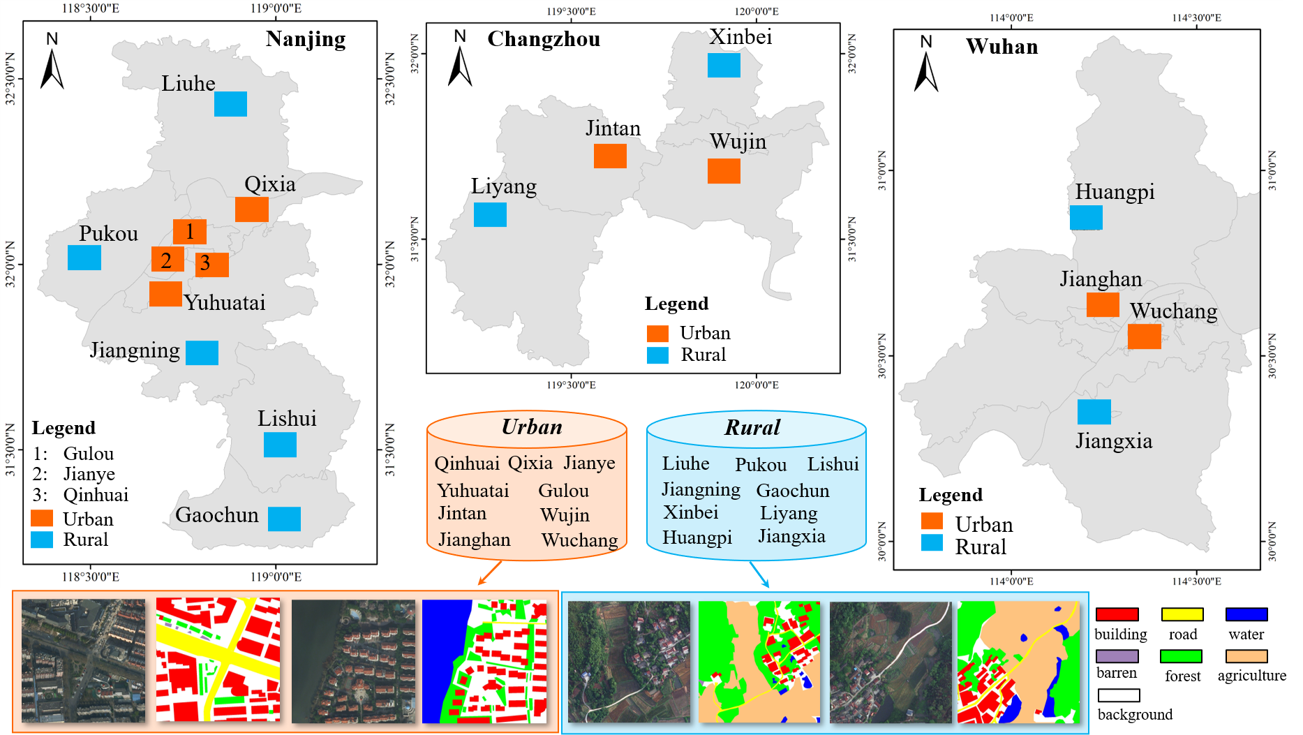
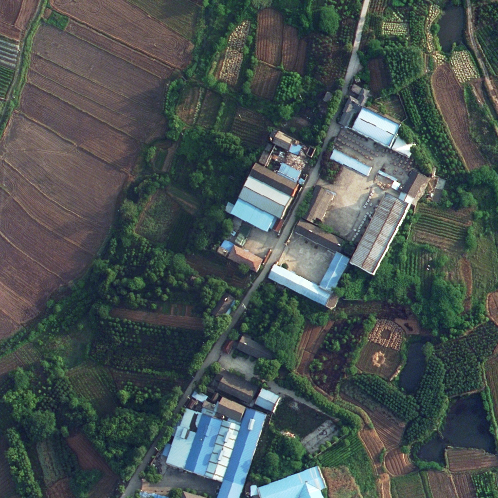
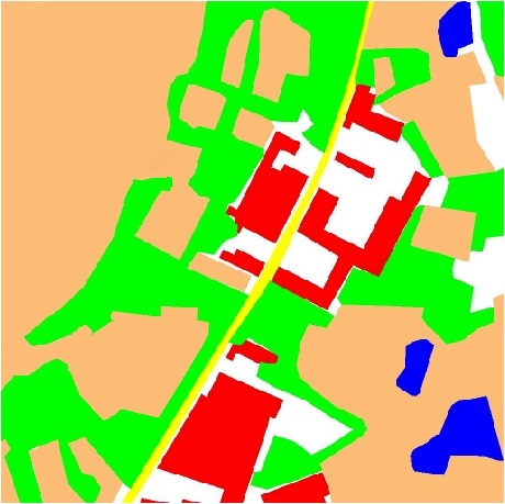
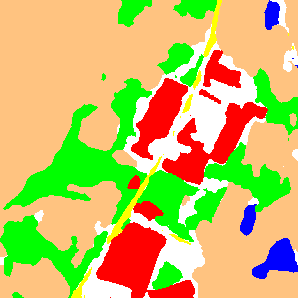
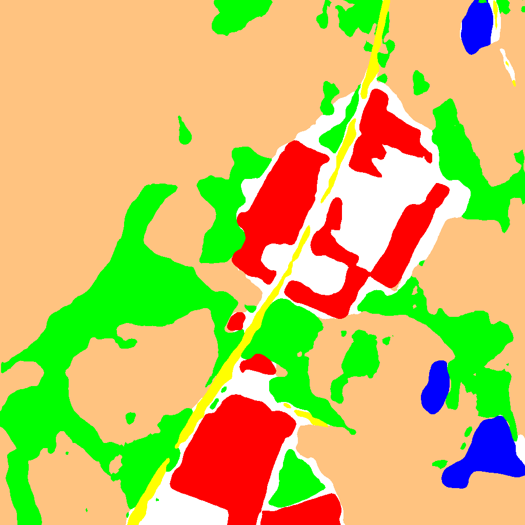
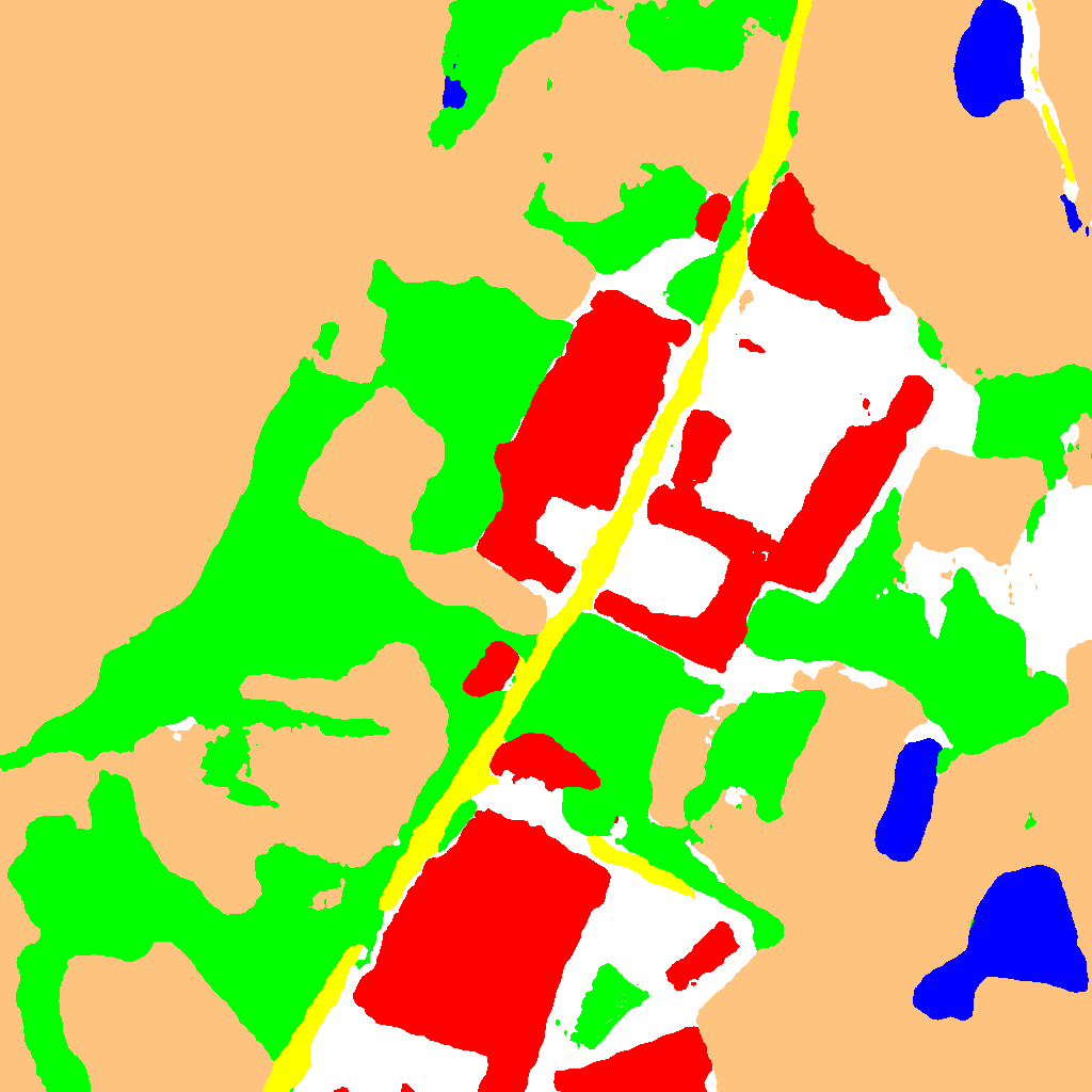
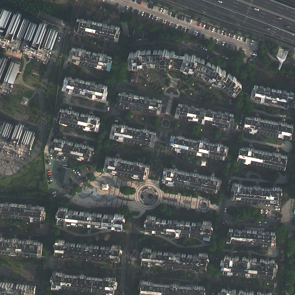
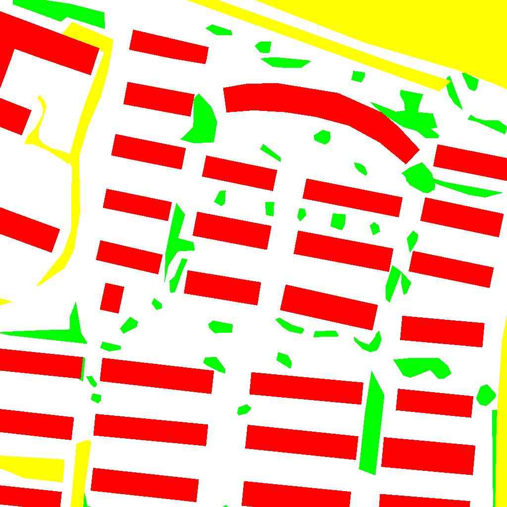
The LoveDA dataset was constructed using 0.3 m images obtained from Nanjing, Changzhou and Wuhan in July 2016, totally covering 536.15 (Figure 1). The historical images were obtained from the Google Earth platform. As each research area has its own planning strategy, the urban-rural ratio is inconsistent [52].
Data from the rural and urban areas were collected referring to the “Urban and Rural Division Code” issued by the National Bureau of Statistics. There are nine urban areas selected from different economically developed districts, which are all densely populated ( 1000 ) [52]. The other nine rural areas were selected from undeveloped districts. The spatial resolution is 0.3 m, with red, green, and blue bands. After geometric registration and pre-processing, each area is covered by images, without overlap. Considering Tobler’s First Law, i.e., everything is related to everything else, but near things are more related than distant things [37], the training, validation, and test sets were split so that they were spatially independent (Figure 1), thus enhancing the difference between the split sets. There are two tasks that can be evaluated on the LoveDA dataset: 1) Semantic segmentation. There are eight areas for training, and the others are for validation and testing. The training, validation, and test sets cover both urban and rural areas.2) Unsupervised domain adaptation. The UDA process considers two cross-domain adaptation sub-tasks: a) Urban Rural. The images from the Qinhuai, Qixia, Jianghan, and Gulou areas are included in the source training set. The images from Liuhe and Huangpi are included in the validation set. The Jiangning, Xinbei, and Liyang images included in the test set. The Oracle setting is designed to test the upper limit of accuracy in a single domain [31]. Hence, the training images were collected from the Pukou, Lishui, Gaochun, and Jiangxia areas. b) Rural Urban. The images from the Pukou, Lishui, Gaochun, and Jiangxia areas are included in the source training set. The images from Yuhuatai and Jintan are used for the validation set. The Jiangye, Wuchang, and Wujin images are used for the test set. In the Oracle setting, the training images cover the Qinhuai, Qixia, Jianghan, and Gulou areas.
3.2 Statistics for LoveDA
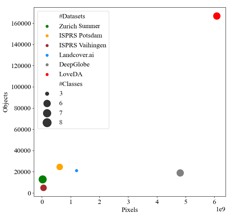
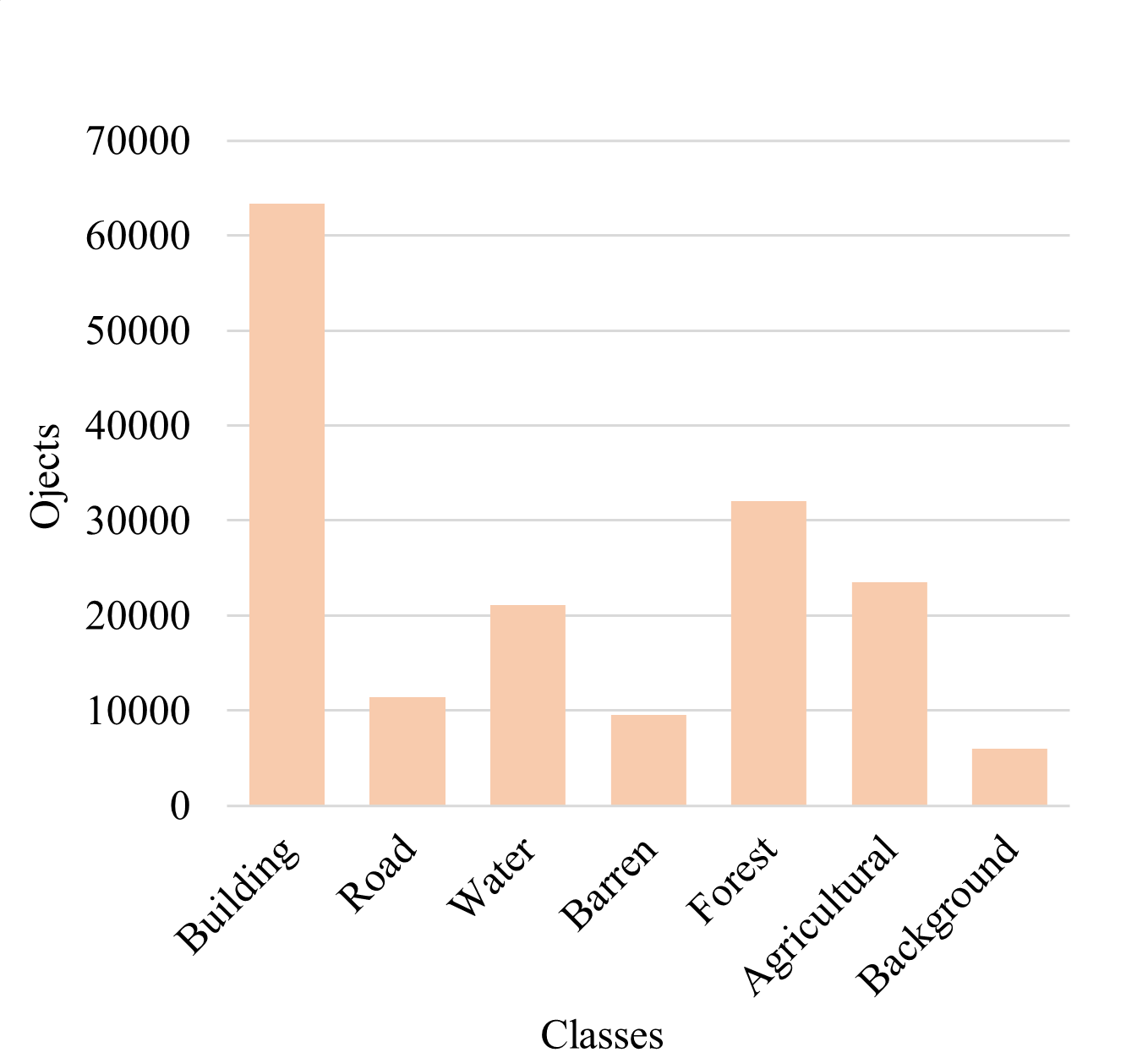
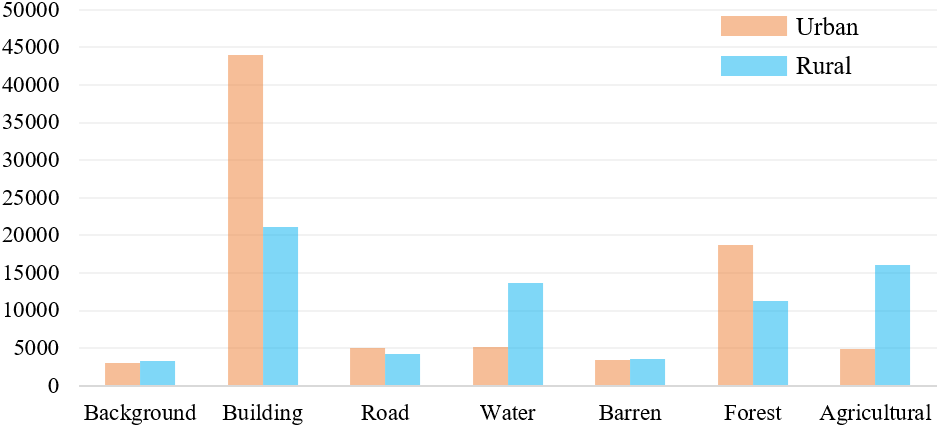
Some statistics of the LoveDA dataset are analyzed in this section. With the collection of public HSR land-cover datasets, the number of labeled objects and pixels has been counted. As is shown in the Figure 2, our proposed LoveDA dataset contains the largest number of labeled pixels as well as land-cover objects, which shows the advantage in data diversity. There are a lot of buildings because urban scenes have large populations (Figure 2). As is shown in Figure 2, the background class contains the most pixels with complex samples [29, 54]. The complex background samples have larger intra-class variance in the complex scenes and cause serious false alarms.
Urban
Rural
3.3 Differences Between Urban and Rural Scenes
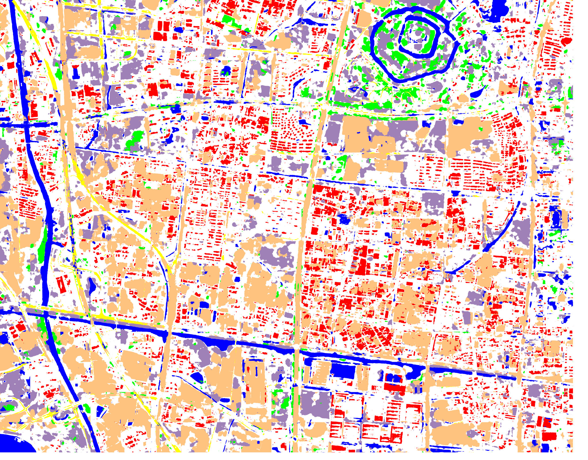
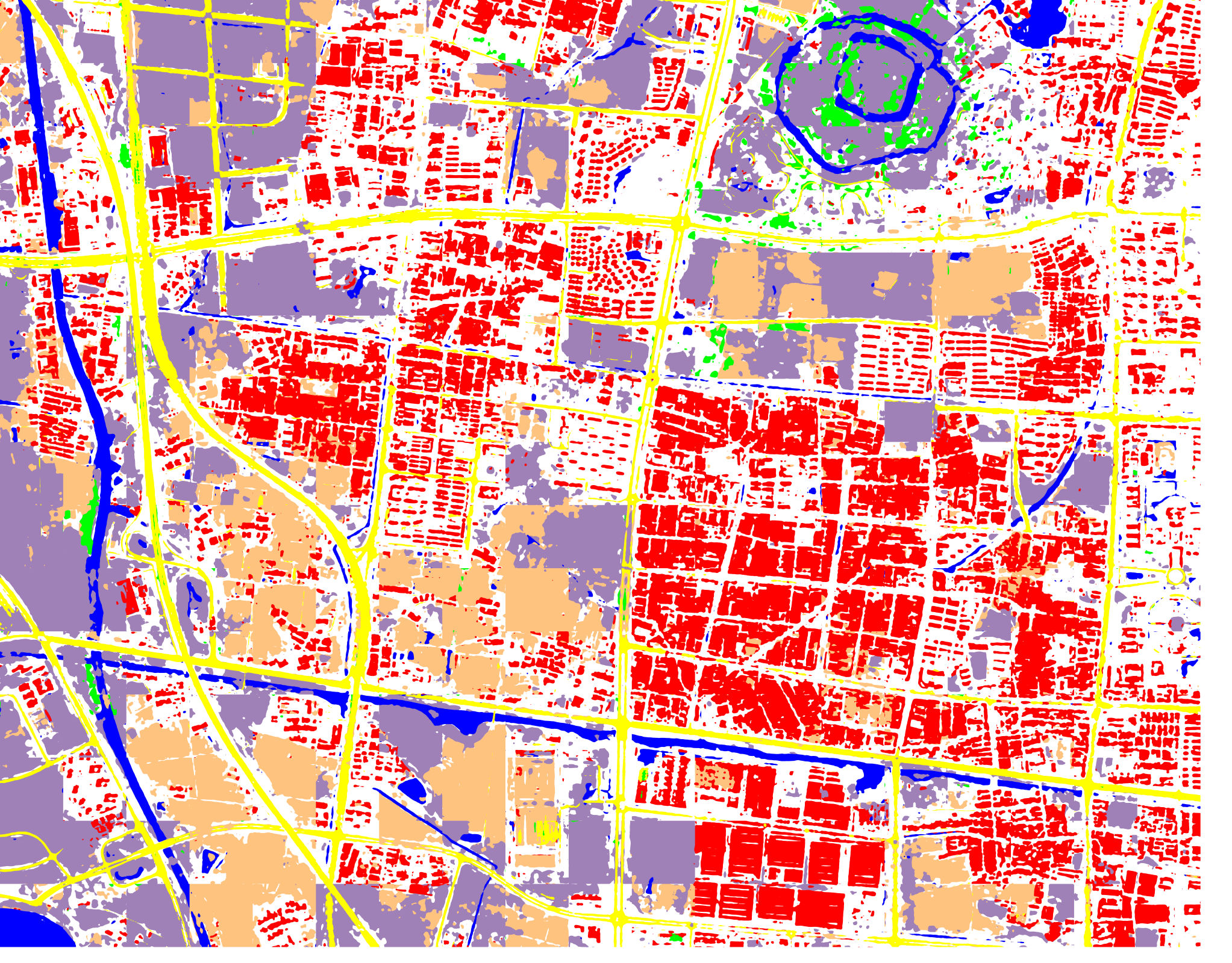
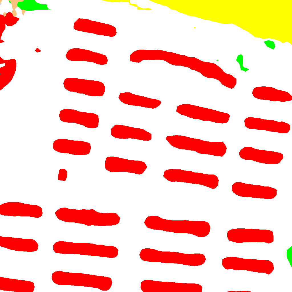
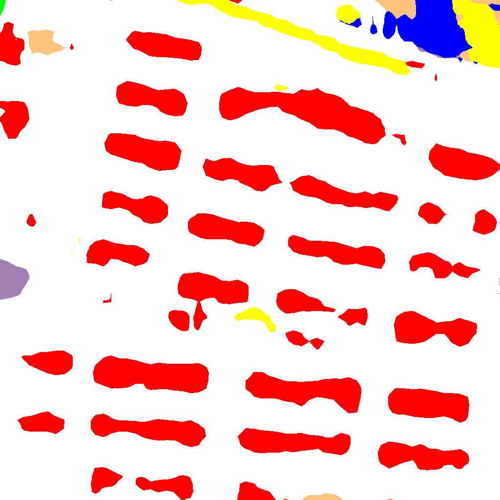
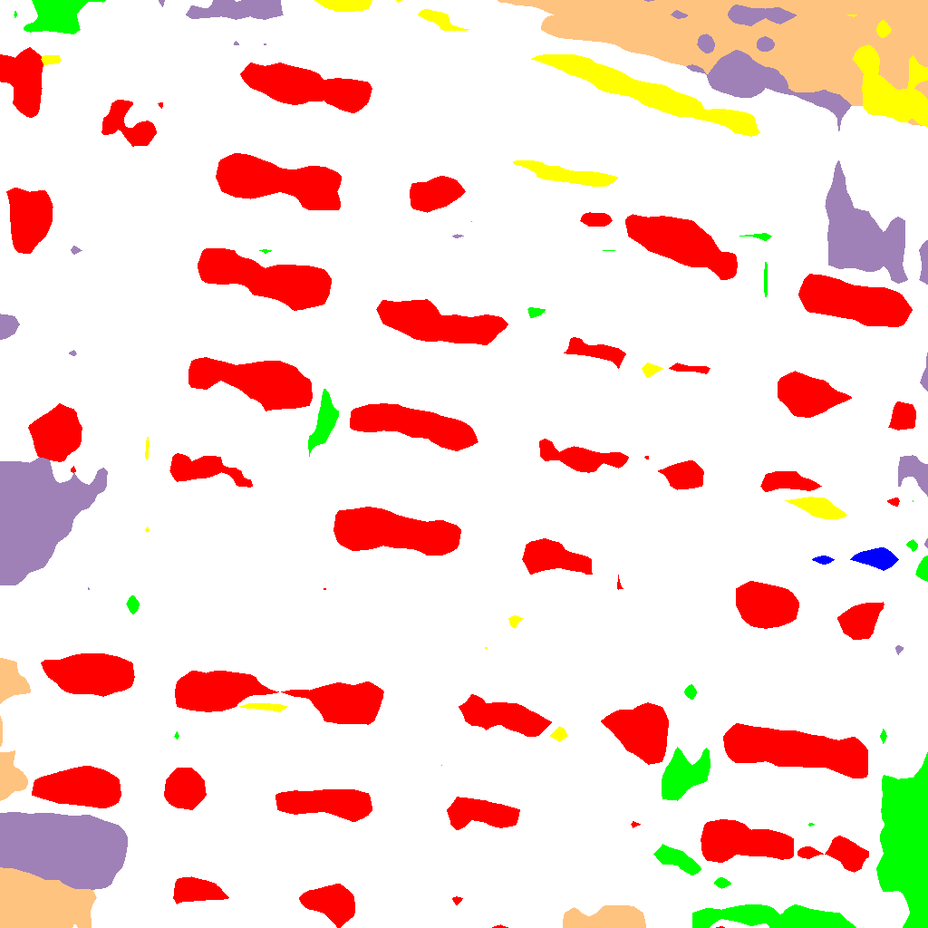
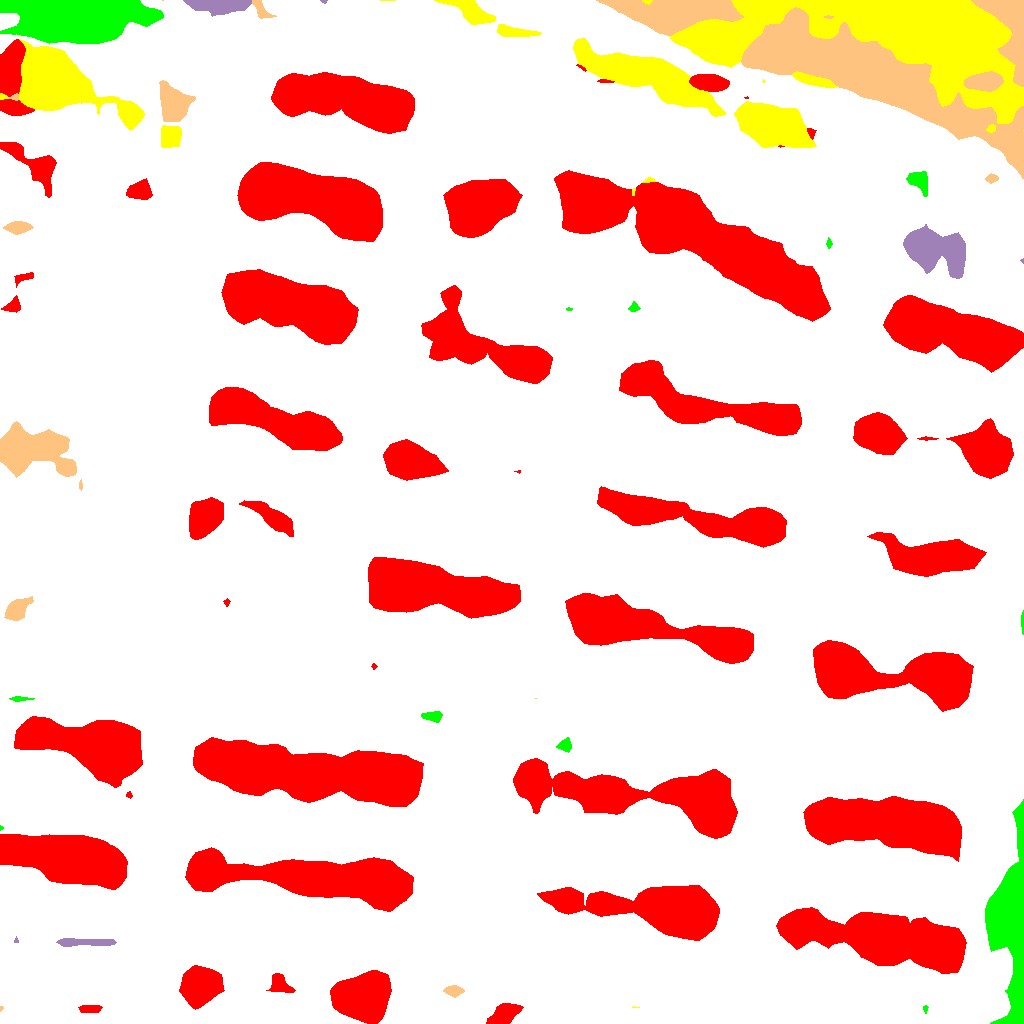
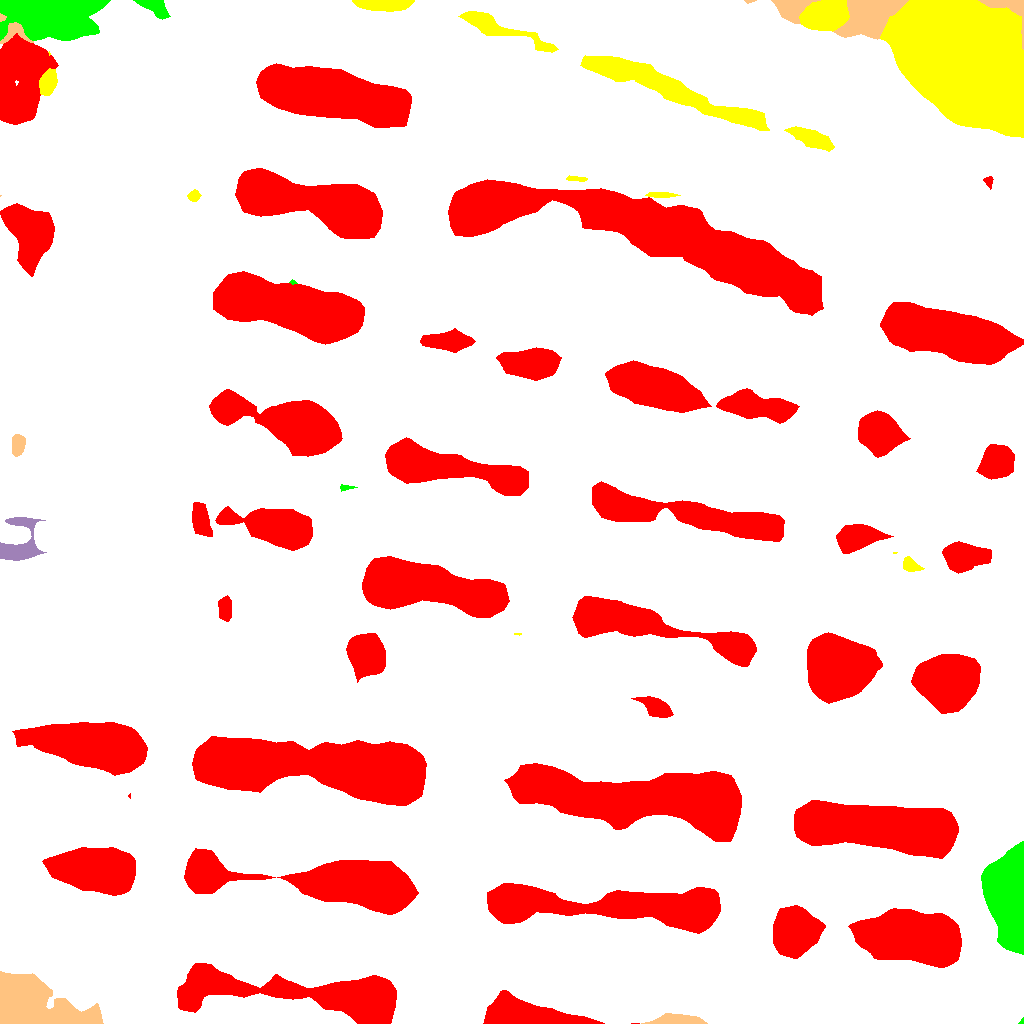
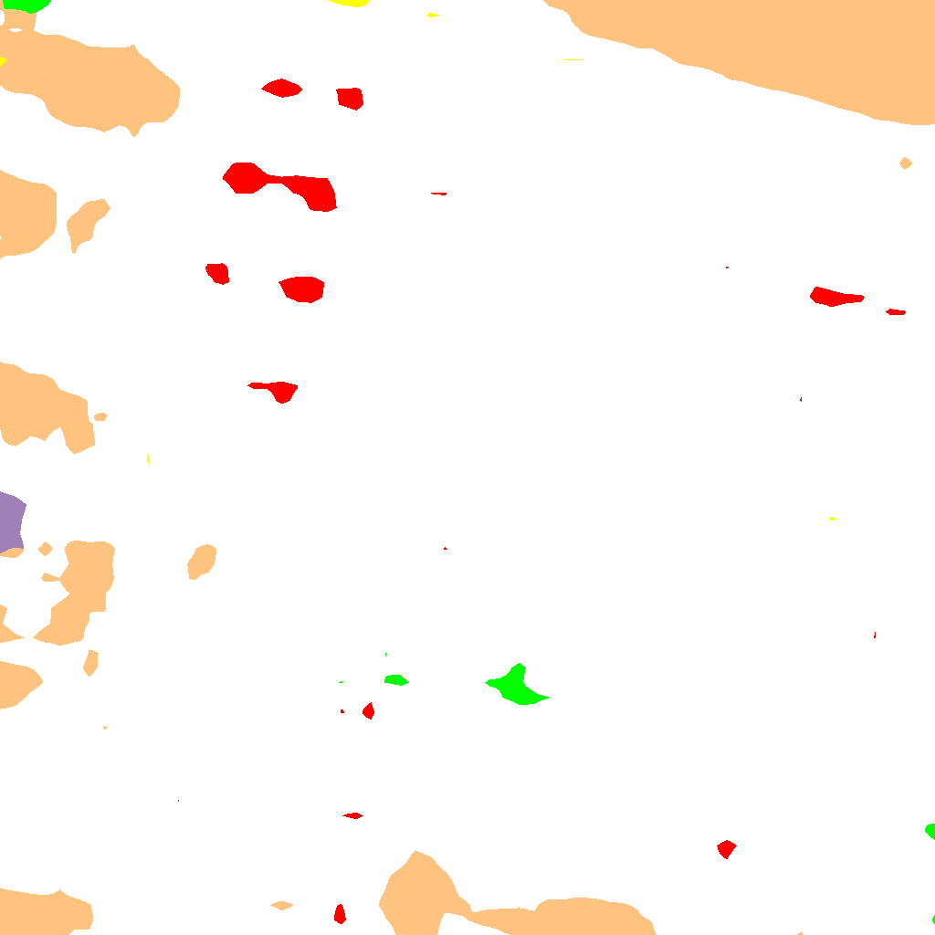
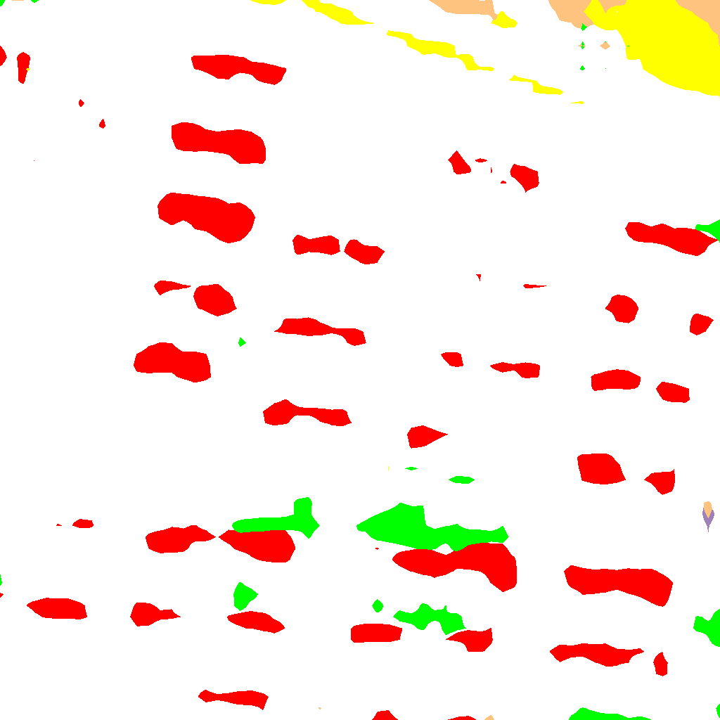
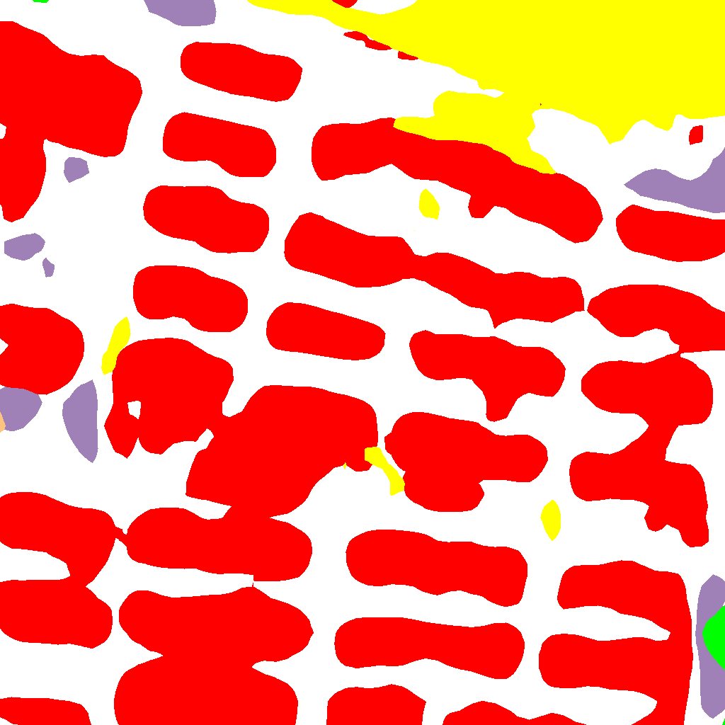
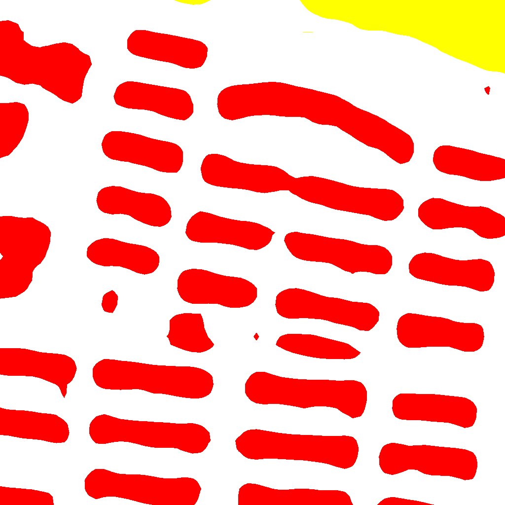
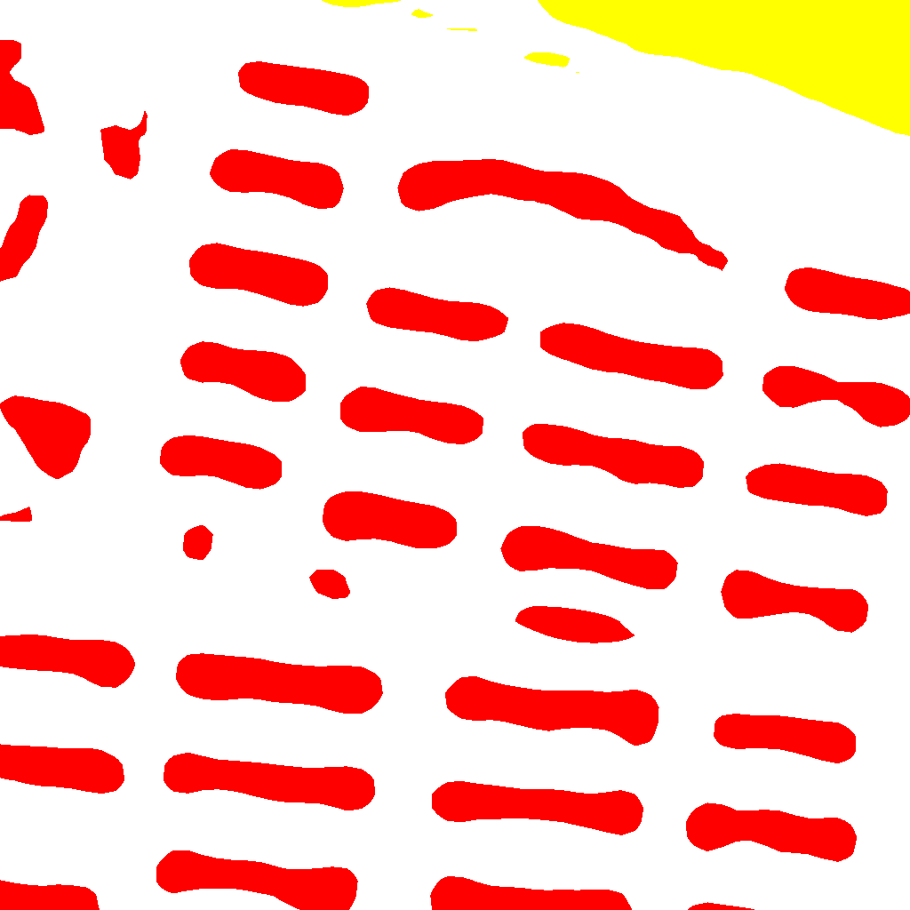
During the process of urbanization, cities differentiate into rural and urban forms. In this section, we list the main differences, which reveal the meaning and challenges of the remote sensing UDA task. For the Nanjing City, the main differences come from the shape, layout, scale, spectra, and class distribution. As is shown in Figure 1, the buildings in the urban area are neatly arranged, with various shapes, while the buildings in the rural area are disordered, with simpler shapes. The roads are wide in the urban scenes. In contrast, the roads are narrow in the rural scenes. Water is often presented in the form of large-scale rivers or lakes in the urban scenes, while small-scale ponds and ditches are common in the rural scenes. The agricultural is found in the gaps between the buildings in the urban scenes, but occurs in a large-scale and continuously distributed form in the rural scenes.
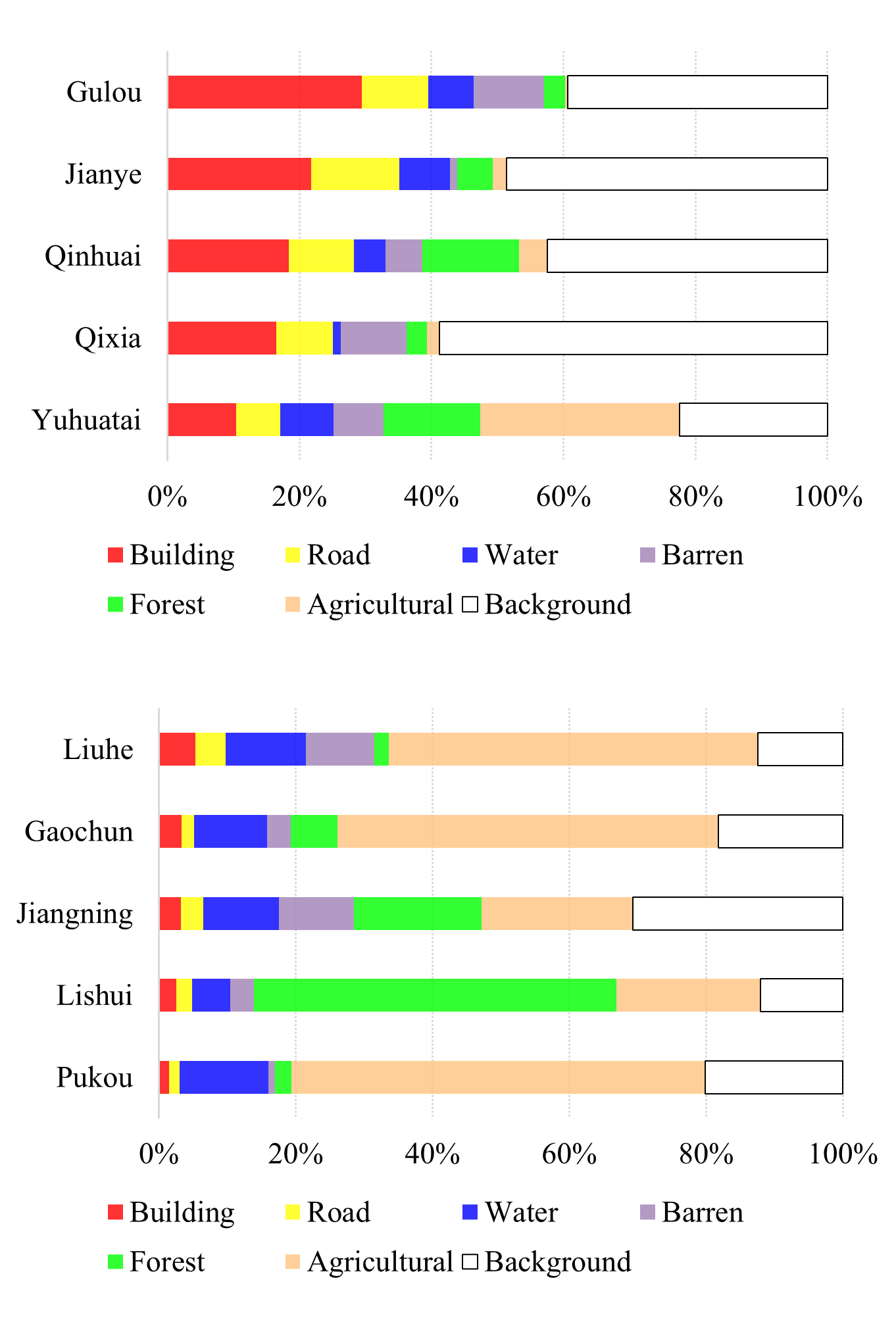
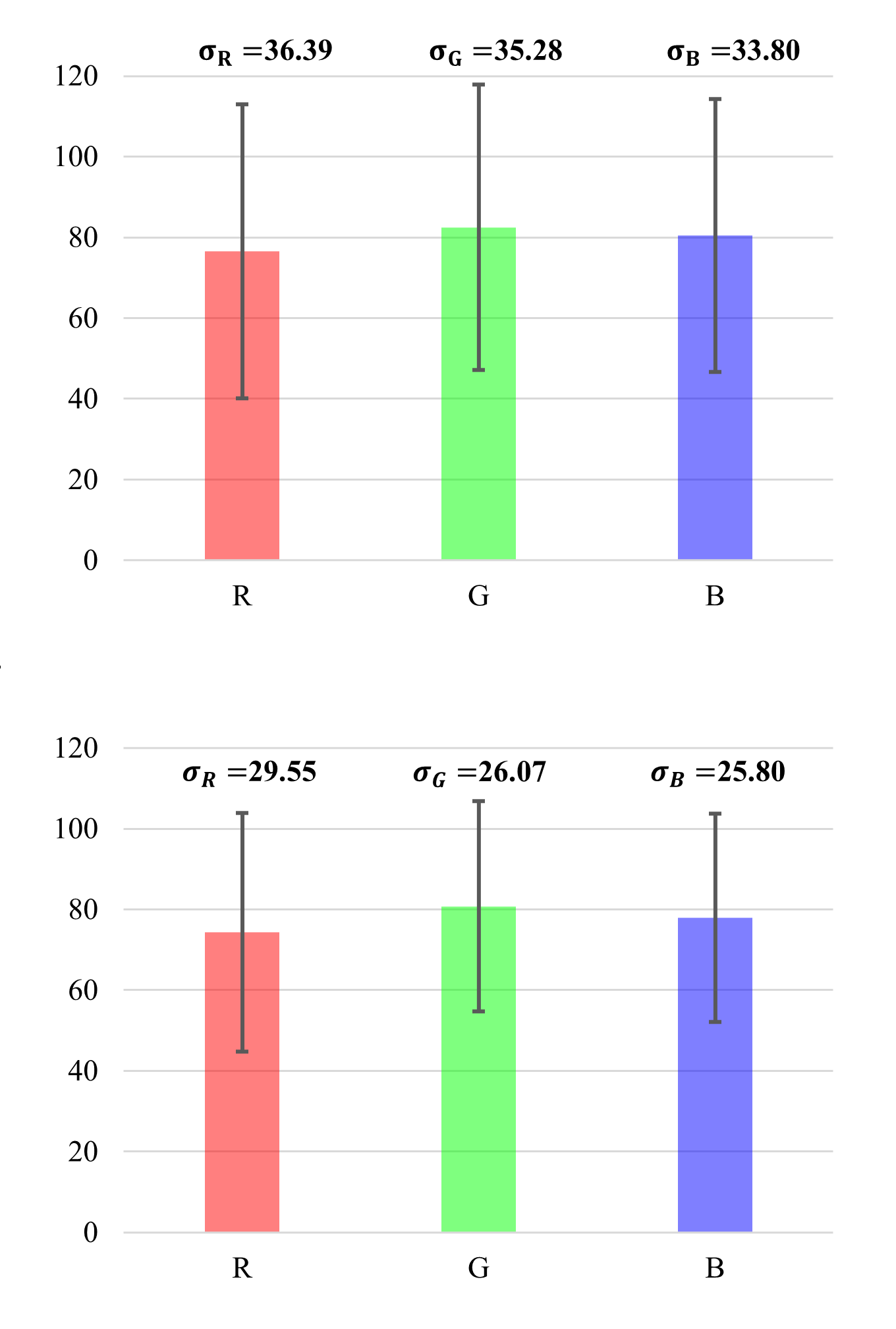
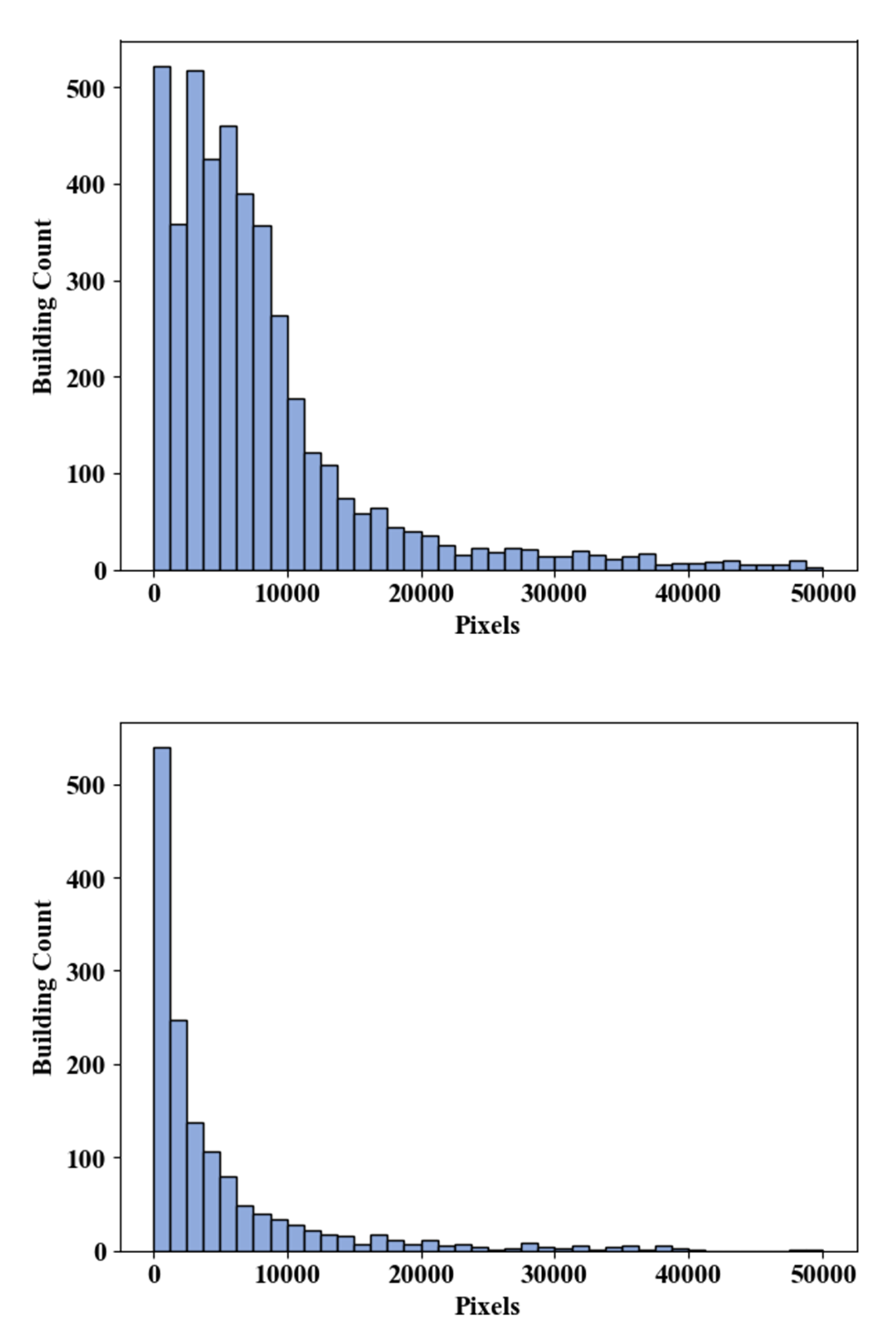
For the class distribution, spectra, and scale, the related statistics are reported in Figure 3. The urban areas always contain more man-made objects such as buildings and roads due to their high population density (Figure 3(a)). In contrast, the rural areas have more agricultural land. The inconsistent class distributions between the urban and rural scenes increases the difficulty of model generalization. For the spectral statistics, the mean values are similar (Figure 3(b)). Because of the large-scale homogeneous geographical areas, such as agriculture and water, the rural images have lower standard deviations. As is shown in Figure 3(c), most of the buildings have relatively small scales in the rural areas, representing the “long tail” phenomenon. However, the buildings in the urban scenes have a larger size variance. Scale differences also exist in the other categories, as shown in Figure 1. The multi-scale objects require the models to have multi-scale capture capabilities. When faced with large-scale land cover mapping tasks, the differences between urban and rural scenes bring new challenges to the model transferability.
4 Experiments
4.1 Semantic Segmentation
For the semantic segmentation task, the general architectures as well as their variants, and particularly those most often used in remote sensing, were tested on the LoveDA dataset. Specifically, the selected networks were: UNet[32], UNet++[55], LinkNet[3], DeepLabV3+[5], PSPNet[53], FCN8S[19], PAN[17], Semantic-FPN[16], HRNet[45], FarSeg[54], and FactSeg[23]. Following the common practice[45, 19], we use the intersection over union (IoU) to report the semantic segmentation accuracy. With respect to the IoU for each class, the mIoU represents the mean of the IoUs over all the categories. The inference speed is reported with a single input (repeated times), using frames per second (FPS).
| Method | Backbone | IoU per category (%) | mIoU (%) | Speed (FPS) | ||||||
| Background | Building | Road | Water | Barren | Forest | Agriculture | ||||
| FCN8S [19] | VGG16 | 42.60 | 49.51 | 48.05 | 73.09 | 11.84 | 43.49 | 58.30 | 46.69 | 86.02 |
| DeepLabV3+ [5] | ResNet50 | 42.97 | 50.88 | 52.02 | 74.36 | 10.40 | 44.21 | 58.53 | 47.62 | 75.33 |
| PAN [17] | ResNet50 | 43.04 | 51.34 | 50.93 | 74.77 | 10.03 | 42.19 | 57.65 | 47.13 | 61.09 |
| UNet [32] | ResNet50 | 43.06 | 52.74 | 52.78 | 73.08 | 10.33 | 43.05 | 59.87 | 47.84 | 71.35 |
| UNet++ [55] | ResNet50 | 42.85 | 52.58 | 52.82 | 74.51 | 11.42 | 44.42 | 58.80 | 48.20 | 27.22 |
| Semantic-FPN [16] | ResNet50 | 42.93 | 51.53 | 53.43 | 74.67 | 11.21 | 44.62 | 58.68 | 48.15 | 73.98 |
| PSPNet [53] | ResNet50 | 44.40 | 52.13 | 53.52 | 76.50 | 9.73 | 44.07 | 57.85 | 48.31 | 74.81 |
| LinkNet [3] | ResNet50 | 43.61 | 52.07 | 52.53 | 76.85 | 12.16 | 45.05 | 57.25 | 48.50 | 67.01 |
| FarSeg [54] | ResNet50 | 43.09 | 51.48 | 53.85 | 76.61 | 9.78 | 43.33 | 58.90 | 48.15 | 66.99 |
| FactSeg [23] | ResNet50 | 42.60 | 53.63 | 52.79 | 76.94 | 16.20 | 42.92 | 57.50 | 48.94 | 65.58 |
| HRNet [45] | W32 | 44.61 | 55.34 | 57.42 | 73.96 | 11.07 | 45.25 | 60.88 | 49.79 | 16.74 |
| Method | mIoU(%) | ||
| Baseline | +MSTr | +MSTrTe | |
| DeepLabV3+ | 47.62 | 49.97 | 51.18 |
| UNet | 48.00 | 50.21 | 51.13 |
| SFPN | 48.15 | 50.80 | 51.82 |
| HRNet | 49.79 | 51.51 | 52.14 |

Implementation details. The data splits followed the Table 8 in §A.1. During the training, we used the Stochastic Gradient Descent (SGD) optimizer with a momentum of and a weight decay of . The learning rate was initially set to , and a ‘poly’ schedule with power was applied. The number of training iterations was set to with a batch size of . For the data augmentation, patches were randomly cropped from the raw images, with random mirroring and rotation. The backbones used in all the networks were pre-trained on ImageNet.
Multi-scale architectures and strategies. As ground objects show considerable scale variance, especially in complex scenes (§3.3), we have analyzed the multi-scale architectures and strategies. There are three noticeable observations from Table 2: 1) UNet++ outperforms UNet due to its nested cross-scale connections between different scales. 2) Among the different fusion strategies, UNet++, Semantic-FPN, LinkNet and HRNet outperform DeepLabV3+. This demonstrates that the cross-layer fusion works better than the in-module fusion. 3) HRNet outperforms the other methods, due to its sophisticated architecture, where the features are repeatedly exchanged across different scales. As is shown in Table 3, multi-scale augmentation (with ) was conducted during the training (MSTr), significantly improving the performance of different methods. In the implementation, the multi-scale inference adopts multi-scale inputs and ensembles the rescaled multiple outputs using a simple mean function. With further use in the testing process, all methods were further improved. As for multi-scale fusion, hierarchical multi-scale architecture search [46] may also become an effective solution.
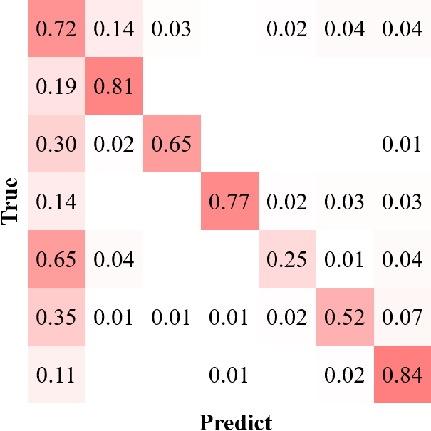
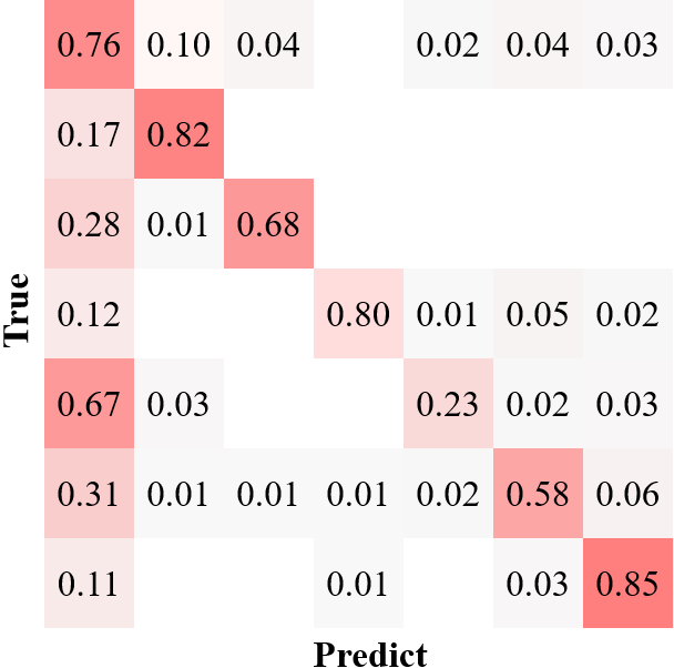
Additional background supervision. The complex background samples cause serious false alarms in HRS imagery semantic segmentation [54, 12]. As is shown in Figure 4, the confusion matrices show that lots of objects were misclassified into background, which is consistent with our analysis in §3.2. Based on Semantic-FPN, we designed the additional background supervision to address this problem. Dice loss [26] and binary cross-entropy loss were utilized with the corresponding modulation factors. We calculated the total loss as: , where denotes the original cross-entropy loss. Table 5 and Table 5 additionally report the precision (P), recall (R) and F1-score (F1) of the background class with varying modulation factors. Besides, the standard deviations are reported after runs. Table 5 shows that the addition of binary cross-entropy loss improves the background accuracy and the overall performance. The combination of and performs well because they optimize the background class from different directions. In the future, the spatial attention mechanism [27] may improve the background with adaptive weights.
| Background | mIoU (%) | |||
| P (%) | R (%) | F1(%) | ||
| 0 | 55.46 | 61.01 | 59.86 | 48.15 0.17 |
| 0.2 | 57.70 | 63.36 | 60.39 | 48.50 0.13 |
| 0.5 | 56.92 | 65.86 | 61.06 | 48.85 0.15 |
| 0.7 | 57.73 | 64.62 | 61.98 | 48.74 0.19 |
| 0.9 | 57.30 | 64.05 | 60.48 | 48.26 0.14 |
| 1.0 | 58.43 | 62.64 | 60.46 | 48.14 0.18 |
| Background | mIoU (%) | ||||
| P (%) | R (%) | F1(%) | |||
| 0.2 | 0.5 | 56.68 | 64.82 | 60.47 | 48.97 0.16 |
| 0.5 | 0.5 | 56.88 | 65.16 | 60.96 | 49.23 0.09 |
| 0.7 | 0.5 | 57.13 | 65.31 | 60.93 | 49.68 0.14 |
| 0.2 | 0.7 | 56.91 | 66.03 | 61.13 | 49.69 0.17 |
| 0.5 | 0.7 | 57.14 | 66.21 | 61.34 | 50.08 0.15 |
| 0.7 | 0.7 | 56.68 | 65.52 | 60.78 | 49.48 0.13 |
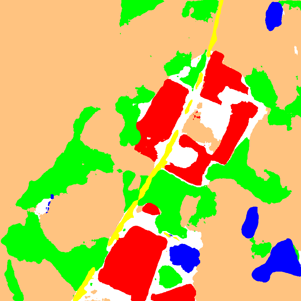
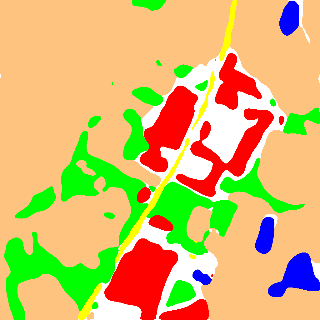
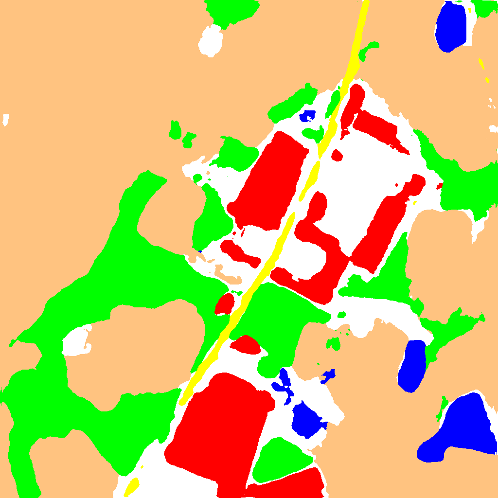
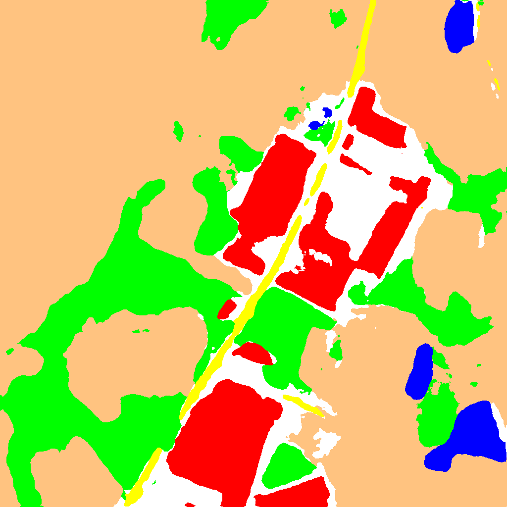
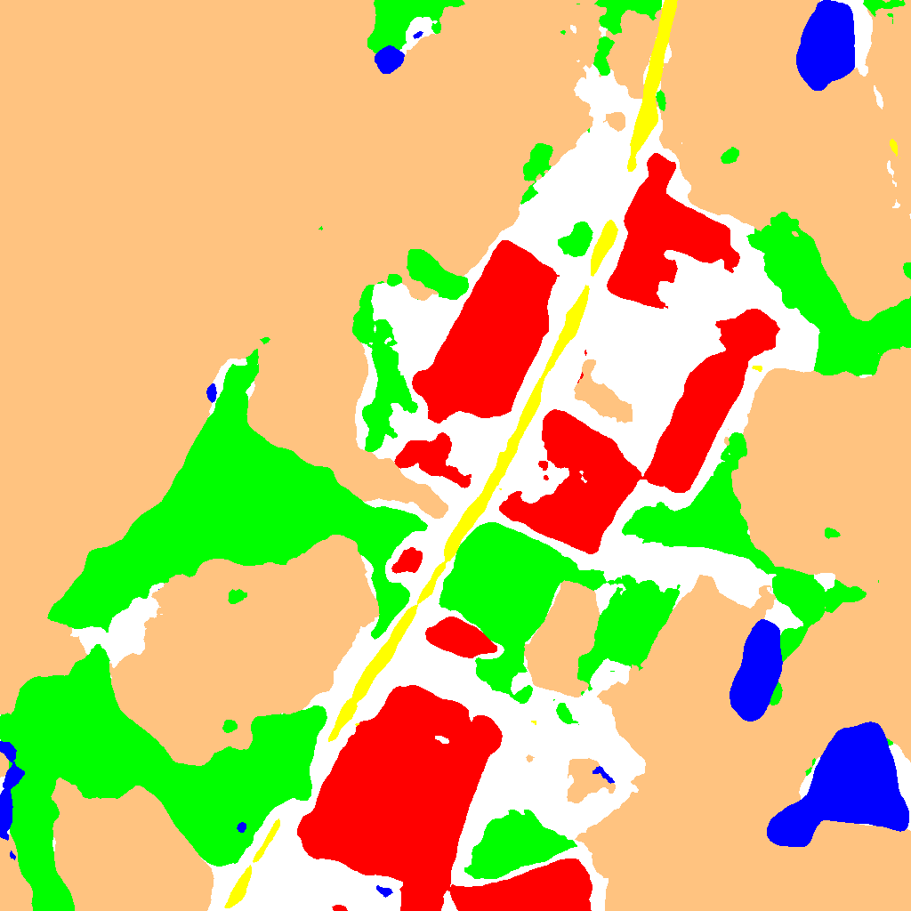
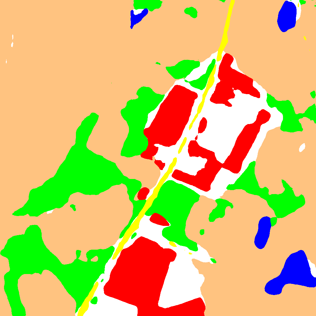
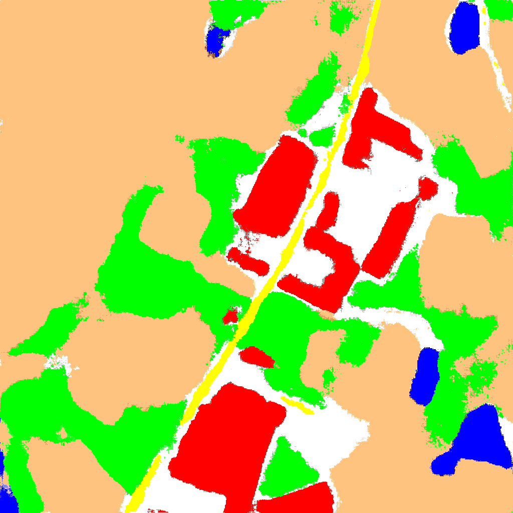

Visualization. Some representative results are shown in Figure 5. With the shallow backbone (VGG16), FCN8S can hardly recognize the road due to its lack of feature extraction capability. The other methods which utilize deep layers can produce better results. Because of the disorderly arrangement and varied scales, the edges of the buildings are hard to extract accurately. Some small-scale objects such as buildings and scattered trees are easy to miss. In contrast, water class achieves higher accuracies for all methods. This because water have strong spectral homogeneity and low intra-class variance [38]. The forest is easy to misclassify into agriculture because these classes have similar spectra. Because of the high-resolution retention and multi-scale fusion, HRNet produces the best visualization result, especially in the details.
4.2 Unsupervised Domain Adaptation
The advanced UDA methods were evaluated on the LoveDA dataset. In addition to the original metric-based approach of DDC [40], two mainstream UDA approaches were tested, i.e., adversarial training (AdaptSeg [39], CLAN [22], TransNorm [47], FADA [44]) and self-training (CBST [56], PyCDA [18], IAST [25]).
| Domain | Method | Type | IoU (%) | mIoU(%) | ||||||
| Background | Building | Road | Water | Barren | Forest | Agriculture | ||||
| Rural Urban | Oracle | - | 48.18 | 52.14 | 56.81 | 85.72 | 12.34 | 36.70 | 35.66 | 46.79 |
| Source only | - | 43.30 | 25.63 | 12.70 | 76.22 | 12.52 | 23.34 | 25.14 | 31.27 | |
| DDC [40] | - | 43.60 | 15.37 | 11.98 | 79.07 | 14.13 | 33.08 | 23.47 | 31.53 | |
| AdaptSeg [39] | AT | 42.35 | 23.73 | 15.61 | 81.95 | 13.62 | 28.70 | 22.05 | 32.68 | |
| FADA [44] | AT | 43.89 | 12.62 | 12.76 | 80.37 | 12.70 | 32.76 | 24.79 | 31.41 | |
| CLAN [22] | AT | 43.41 | 25.42 | 13.75 | 79.25 | 13.71 | 30.44 | 25.80 | 33.11 | |
| TransNorm [47] | AT | 38.37 | 5.04 | 3.75 | 80.83 | 14.19 | 33.99 | 17.91 | 27.73 | |
| PyCDA [18] | ST | 38.04 | 35.86 | 45.51 | 74.87 | 7.71 | 40.39 | 11.39 | 36.25 | |
| CBST [56] | ST | 48.37 | 46.10 | 35.79 | 80.05 | 19.18 | 29.69 | 30.05 | 41.32 | |
| IAST [25] | ST | 48.57 | 31.51 | 28.73 | 86.01 | 20.29 | 31.77 | 36.50 | 40.48 | |
| Urban Rural | Oracle | - | 37.18 | 52.74 | 43.74 | 65.89 | 11.47 | 45.78 | 62.91 | 45.67 |
| Source only | - | 24.16 | 37.02 | 32.56 | 49.42 | 14.00 | 29.34 | 35.65 | 31.74 | |
| DDC [40] | - | 25.61 | 44.27 | 31.28 | 44.78 | 13.74 | 33.83 | 25.98 | 31.36 | |
| AdaptSeg [39] | AT | 26.89 | 40.53 | 30.65 | 50.09 | 16.97 | 32.51 | 28.25 | 32.27 | |
| FADA [44] | AT | 24.39 | 32.97 | 25.61 | 47.59 | 15.34 | 34.35 | 20.29 | 28.65 | |
| CLAN [22] | AT | 22.93 | 44.78 | 25.99 | 46.81 | 10.54 | 37.21 | 24.45 | 30.39 | |
| TransNorm [47] | AT | 19.39 | 36.30 | 22.04 | 36.68 | 14.00 | 40.62 | 3.30 | 24.62 | |
| PyCDA [18] | ST | 12.36 | 38.11 | 20.45 | 57.16 | 18.32 | 36.71 | 41.90 | 32.14 | |
| CBST [56] | ST | 25.06 | 44.02 | 23.79 | 50.48 | 8.33 | 39.16 | 49.65 | 34.36 | |
| IAST [25] | ST | 29.97 | 49.48 | 28.29 | 64.49 | 2.13 | 33.36 | 61.37 | 38.44 | |
-
The abbreviations are: AT – adversarial training methods. ST – self-training methods.
Implementation details. All the UDA methods adopted the same feature extractor and discriminator, following the common practice [39, 22, 44]. Specifically, DeepLabV2 [4] with ResNet50 was utilized as the extractor, and the discriminator was constructed by fully convolutional layers [39]. For the adversarial training (AT), the classification and discriminator learning rates were set to and , respectively. The Adam optimizer was used for the discriminator with the momentum of and . The number of training iterations was set to , with a batch size of . The eight source images and eight target images were alternatively input. The other settings are the same in the semantic segmentation. and the learning schedule is the same as in semantic segmentation settings. For the self-training (ST), the classification learning rate was set to . Full implementation details are provided in the §A.4.
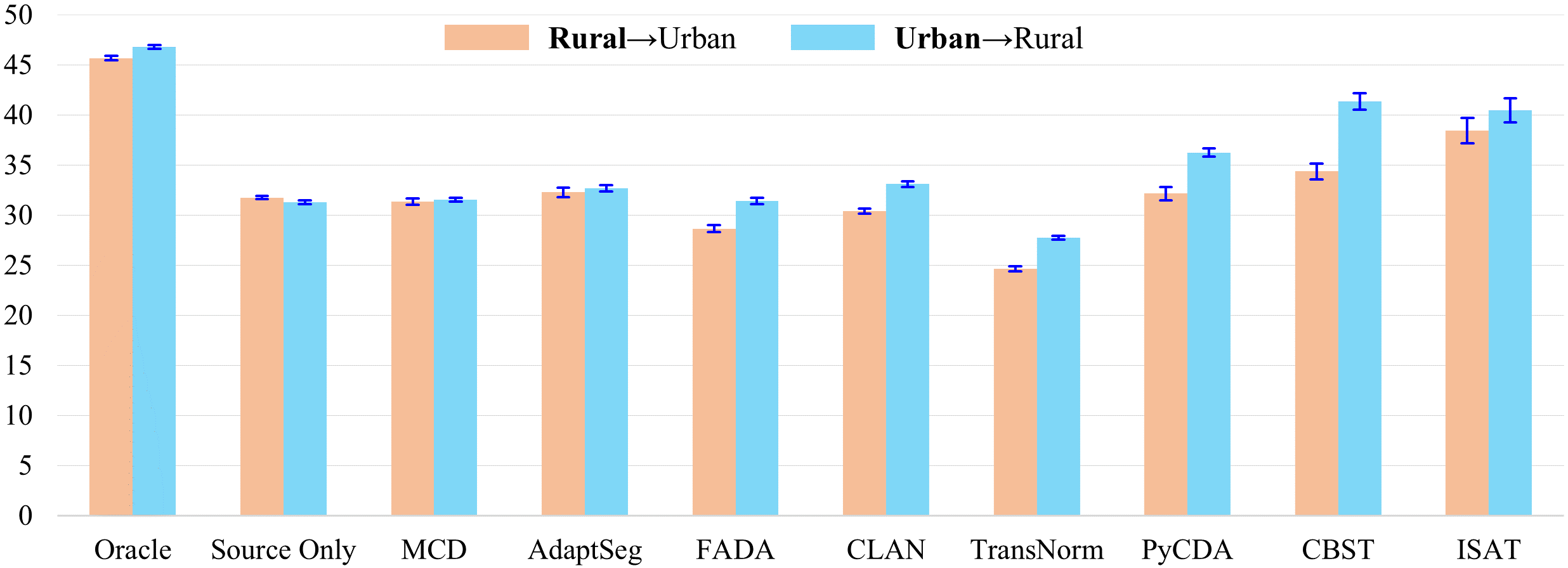
Benchmark results. As is shown in Table 6, the Oracle setting obtains the best overall performances. However, DeepLabV2 has lost its effectiveness due to the domain divergence, referring to the result of Source only setting. In the Rural Urban experiments, the accuracies of artificial classes (building and road) drop more than natural classes (forest and agricultural). Because of the inconsistent class distribution, the Urban Rural experiments show the opposite results. The transfer learning methods relatively improve the model transferability. Noticeably, TransNorm obtains the lowest mIoUs. This is because the source and target images were obtained by the same sensor, and their spectral statistics are similar (Figure 3(2)). These rural and urban domains require similar normalization weights, so that the adaptive normalization can lead to optimization conflicts (more analysis are provided in §A.6). The ST methods achieve better performances because they address the class imbalance problem with pseudo-label generation.
Inconsistent class distributions. It is noticeable to find that the ST methods surpass AT methods in cross-domain adaptation experiments. We conclude that the main reason for this is the extremely inconsistent class distribution (Figure 3(a)). The rural scenes only contain a few artificial samples and large-scale natural objects. In contrast, the urban scenes have a mixture of buildings and roads with few natural objects. The AT methods cannot address this difficulty, so that they report lower accuracies. However, differing from the AT methods, the ST methods generate pseudo-labels on the target images. With the addition of diverse target samples, the class distribution divergence is eliminated during the training. Overall, the ST methods show more potential in the UDA land-cover semantic segmentation task. In Urban Rural experiments, all UDA methods show negative transfer effects for the road class. Hence, more tailored UDA methods are worth exploring faced with these special challenges.
Visualization. The qualitative results for the Rural Urban experiments are shown in Figure 6. The Oracle result successfully recognizes the buildings and roads, and is the closest to the ground truth. According to the Table 2, it can be further improved by using a more robust backbone. The ST methods (j)–(l) produce better results than AT methods (f)–(i), but there is still much room for improvement. The large-scale mapping visualizations are provided in §A.7.
Pseudo-label analysis for CBST. As pseudo samples are important for addressing inconsistent class distribution problem, we varied the target class proportion in CBST, which is a hyper-parameter controlling the number of pseudo samples. The mean F1-score (mF1) and mIoU are reported in Table 7. Without pseudo-label learning (), the model degenerated into Source only setting and achieved low accuracy. The optimal range of is relatively large (), which proves that it is not sensitive to the remote sensing UDA task.
| 0. | 0.01 | 0.05 | 0.1 | 0.5 | 0.7 | 0.9 | 1.0 | |
| mF1(%) | 46.81 | 45.24 | 48.50 | 50.93 | 56.30 | 51.23 | 51.03 | 49.43 |
| mIoU(%) | 32.94 | 32.18 | 34.46 | 36.84 | 41.32 | 37.12 | 37.02 | 35.47 |
5 Conclusion
The differences between urban and rural scenes limit the generalization of deep learning approaches in land-cover mapping. In order to address this problem, we built an HSR dataset for Land-cOVEr Domain Adaptive semantic segmentation (LoveDA). The LoveDA dataset reflects three challenges in large-scale remote sensing mapping, including multi-scale objects, complex background samples, and inconsistent class distributions. The state-of-the-art methods were evaluated on the LoveDA dataset, revealing the challenges of LoveDA. In addition, multi-scale architectures and strategies, additional background supervision and pseudo-label analysis were conducted to find alternative ways to address these challenges.
6 Broader Impact
This work offers a free and open dataset with the purpose of advancing land-cover semantic segmentation in the area of remote sensing. We also provide two benchmarked tasks with three considerable challenges. This will allow other researchers to easily build on this work and create new and enhanced capabilities. The authors do not foresee any negative societal impacts of this work. A potential positive societal impact may arise from the development of generalizable models that can produce large-scale high-spatial-resolution land-cover mapping accurately. This could help to reduce the manpower and material resource consumption of surveying and mapping.
7 Acknowledgments
This work was supported by National Key Research and Development Program of China under Grant No. 2017YFB0504202, National Natural Science Foundation of China under Grant Nos. 41771385, 41801267, and the China Postdoctoral Science Foundation under Grant 2017M622522. This work was supported by the Nanjing Bureau of Surveying and Mapping.
References
- [1] H. Alemohammad and K. Booth. LandCoverNet: A global benchmark land cover classification training dataset. arXiv preprint arXiv:2012.03111, 2020.
- [2] A. Boguszewski, D. Batorski, N. Ziemba-Jankowska, T. Dziedzic, and A. Zambrzycka. LandCover.ai: Dataset for automatic mapping of buildings, woodlands, water and roads from aerial imagery. In Proceedings of the IEEE/CVF Conference on Computer Vision and Pattern Recognition, pages 1102–1110, 2021.
- [3] A. Chaurasia and E. Culurciello. Linknet: Exploiting encoder representations for efficient semantic segmentation. In 2017 IEEE Visual Communications and Image Processing (VCIP), pages 1–4. IEEE, 2017.
- [4] L.-C. Chen, G. Papandreou, I. Kokkinos, K. Murphy, and A. L. Yuille. Deeplab: Semantic image segmentation with deep convolutional nets, atrous convolution, and fully connected crfs. IEEE transactions on pattern analysis and machine intelligence, 40(4):834–848, 2017.
- [5] L.-C. Chen, Y. Zhu, G. Papandreou, F. Schroff, and H. Adam. Encoder-decoder with atrous separable convolution for semantic image segmentation. In Proceedings of the European conference on computer vision (ECCV), pages 801–818, 2018.
- [6] Q. Chen, L. Wang, Y. Wu, G. Wu, Z. Guo, and S. L. Waslander. Aerial imagery for roof segmentation: A large-scale dataset towards automatic mapping of buildings. ISPRS Journal of Photogrammetry and Remote Sensing, 147:42–55, 2019.
- [7] W. Chen, Z. Jiang, Z. Wang, K. Cui, and X. Qian. Collaborative global-local networks for memory-efficient segmentation of ultra-high resolution images. In Proceedings of the IEEE/CVF Conference on Computer Vision and Pattern Recognition, pages 8924–8933, 2019.
- [8] U. S. Commission et al. A recommendation on the method to delineate cities, urban and rural areas for international statistical comparisons. European Commission, 2020.
- [9] I. Demir, K. Koperski, D. Lindenbaum, G. Pang, J. Huang, S. Basu, F. Hughes, D. Tuia, and R. Raskar. Deepglobe 2018: A challenge to parse the earth through satellite images. In Proceedings of the IEEE Conference on Computer Vision and Pattern Recognition Workshops, pages 172–181, 2018.
- [10] Y. Dong, T. Liang, Y. Zhang, and B. Du. Spectral–spatial weighted kernel manifold embedded distribution alignment for remote sensing image classification. IEEE Transactions on Cybernetics, 51(6):3185–3197, 2020.
- [11] Y. Duan, H. Huang, Z. Li, and Y. Tang. Local manifold-based sparse discriminant learning for feature extraction of hyperspectral image. IEEE transactions on cybernetics, 2020.
- [12] M. Everingham, S. A. Eslami, L. Van Gool, C. K. Williams, J. Winn, and A. Zisserman. The pascal visual object classes challenge: A retrospective. International journal of computer vision, 111(1):98–136, 2015.
- [13] J. Iqbal and M. Ali. Weakly-supervised domain adaptation for built-up region segmentation in aerial and satellite imagery. ISPRS Journal of Photogrammetry and Remote Sensing, 167:263–275, 2020.
- [14] S. Jin, C. Homer, J. Dewitz, P. Danielson, and D. Howard. National land cover database (nlcd) 2016 science research products. In AGU Fall Meeting Abstracts, volume 2019, pages B11I–2301, 2019.
- [15] C. Jun, Y. Ban, and S. Li. Open access to earth land-cover map. Nature, 514(7523):434–434, 2014.
- [16] A. Kirillov, R. Girshick, K. He, and P. Dollár. Panoptic feature pyramid networks. In Proceedings of the IEEE/CVF Conference on Computer Vision and Pattern Recognition, pages 6399–6408, 2019.
- [17] H. Li, P. Xiong, J. An, and L. Wang. Pyramid attention network for semantic segmentation. arXiv preprint arXiv:1805.10180, 2018.
- [18] Q. Lian, F. Lv, L. Duan, and B. Gong. Constructing self-motivated pyramid curriculums for cross-domain semantic segmentation: A non-adversarial approach. In Proceedings of the IEEE/CVF International Conference on Computer Vision, pages 6758–6767, 2019.
- [19] J. Long, E. Shelhamer, and T. Darrell. Fully convolutional networks for semantic segmentation. In Proceedings of the IEEE conference on computer vision and pattern recognition, pages 3431–3440, 2015.
- [20] M. Long, Y. Cao, J. Wang, and M. Jordan. Learning transferable features with deep adaptation networks. In International conference on machine learning, pages 97–105. PMLR, 2015.
- [21] X. Lu, T. Gong, and X. Zheng. Multisource compensation network for remote sensing cross-domain scene classification. IEEE Transactions on Geoscience and Remote Sensing, 58(4):2504–2515, 2019.
- [22] Y. Luo, L. Zheng, T. Guan, J. Yu, and Y. Yang. Taking a closer look at domain shift: Category-level adversaries for semantics consistent domain adaptation. In Proceedings of the IEEE/CVF Conference on Computer Vision and Pattern Recognition, pages 2507–2516, 2019.
- [23] A. Ma, J. Wang, Y. Zhong, and Z. Zheng. Factseg: Foreground activation-driven small object semantic segmentation in large-scale remote sensing imagery. IEEE Transactions on Geoscience and Remote Sensing, 2021.
- [24] D. Marcos, M. Volpi, B. Kellenberger, and D. Tuia. Land cover mapping at very high resolution with rotation equivariant cnns: Towards small yet accurate models. ISPRS journal of photogrammetry and remote sensing, 145:96–107, 2018.
- [25] K. Mei, C. Zhu, J. Zou, and S. Zhang. Instance adaptive self-training for unsupervised domain adaptation. In Computer Vision–ECCV 2020: 16th European Conference, Glasgow, UK, August 23–28, 2020, Proceedings, Part XXVI 16, pages 415–430. Springer, 2020.
- [26] F. Milletari, N. Navab, and S.-A. Ahmadi. V-net: Fully convolutional neural networks for volumetric medical image segmentation. In 2016 fourth international conference on 3D vision (3DV), pages 565–571. IEEE, 2016.
- [27] L. Mou, Y. Hua, and X. X. Zhu. A relation-augmented fully convolutional network for semantic segmentation in aerial scenes. In Proceedings of the IEEE/CVF Conference on Computer Vision and Pattern Recognition, pages 12416–12425, 2019.
- [28] E. Othman, Y. Bazi, F. Melgani, H. Alhichri, N. Alajlan, and M. Zuair. Domain adaptation network for cross-scene classification. IEEE Transactions on Geoscience and Remote Sensing, 55(8):4441–4456, 2017.
- [29] J. Pang, C. Li, J. Shi, Z. Xu, and H. Feng. -CNN: Fast tiny object detection in large-scale remote sensing images. IEEE Transactions on Geoscience and Remote Sensing, 57(8):5512–5524, 2019.
- [30] X. Peng, Q. Bai, X. Xia, Z. Huang, K. Saenko, and B. Wang. Moment matching for multi-source domain adaptation. In Proceedings of the IEEE/CVF International Conference on Computer Vision, pages 1406–1415, 2019.
- [31] X. Peng, B. Usman, N. Kaushik, D. Wang, J. Hoffman, and K. Saenko. Visda: A synthetic-to-real benchmark for visual domain adaptation. In Proceedings of the IEEE Conference on Computer Vision and Pattern Recognition Workshops, pages 2021–2026, 2018.
- [32] O. Ronneberger, P. Fischer, and T. Brox. U-net: Convolutional networks for biomedical image segmentation. In International Conference on Medical image computing and computer-assisted intervention, pages 234–241. Springer, 2015.
- [33] D. Sulla-Menashe and M. A. Friedl. User guide to collection 6 modis land cover (mcd12q1 and mcd12c1) product. USGS: Reston, VA, USA, pages 1–18, 2018.
- [34] B. Sun and K. Saenko. Deep coral: Correlation alignment for deep domain adaptation. In European conference on computer vision, pages 443–450. Springer, 2016.
- [35] O. Tasar, Y. Tarabalka, A. Giros, P. Alliez, and S. Clerc. Standardgan: Multi-source domain adaptation for semantic segmentation of very high resolution satellite images by data standardization. In Proceedings of the IEEE/CVF Conference on Computer Vision and Pattern Recognition Workshops, pages 192–193, 2020.
- [36] C. Tian, C. Li, and J. Shi. Dense fusion classmate network for land cover classification. In Proceedings of the IEEE Conference on Computer Vision and Pattern Recognition Workshops, pages 192–196, 2018.
- [37] W. R. Tobler. A computer movie simulating urban growth in the Detroit region. Economic geography, 46(sup1):234–240, 1970.
- [38] X.-Y. Tong, G.-S. Xia, Q. Lu, H. Shen, S. Li, S. You, and L. Zhang. Land-cover classification with high-resolution remote sensing images using transferable deep models. Remote Sensing of Environment, 237:111322, 2020.
- [39] Y.-H. Tsai, W.-C. Hung, S. Schulter, K. Sohn, M.-H. Yang, and M. Chandraker. Learning to adapt structured output space for semantic segmentation. In Proceedings of the IEEE conference on computer vision and pattern recognition, pages 7472–7481, 2018.
- [40] E. Tzeng, J. Hoffman, N. Zhang, K. Saenko, and T. Darrell. Deep domain confusion: Maximizing for domain invariance. arXiv preprint arXiv:1412.3474, 2014.
- [41] A. Van Etten, D. Lindenbaum, and T. M. Bacastow. Spacenet: A remote sensing dataset and challenge series. arXiv preprint arXiv:1807.01232, 2018.
- [42] H. Venkateswara, J. Eusebio, S. Chakraborty, and S. Panchanathan. Deep hashing network for unsupervised domain adaptation. In Proceedings of the IEEE Conference on Computer Vision and Pattern Recognition, pages 5018–5027, 2017.
- [43] M. Volpi and V. Ferrari. Semantic segmentation of urban scenes by learning local class interactions. In Proceedings of the IEEE Conference on Computer Vision and Pattern Recognition Workshops, pages 1–9, 2015.
- [44] H. Wang, T. Shen, W. Zhang, L.-Y. Duan, and T. Mei. Classes matter: A fine-grained adversarial approach to cross-domain semantic segmentation. In European Conference on Computer Vision, pages 642–659. Springer, 2020.
- [45] J. Wang, K. Sun, T. Cheng, B. Jiang, C. Deng, Y. Zhao, D. Liu, Y. Mu, M. Tan, X. Wang, et al. Deep high-resolution representation learning for visual recognition. IEEE transactions on pattern analysis and machine intelligence, 2020.
- [46] J. Wang, Y. Zhong, Z. Zheng, A. Ma, and L. Zhang. RSNet: the search for remote sensing deep neural networks in recognition tasks. IEEE Transactions on Geoscience and Remote Sensing, 59(3):2520–2534, 2021.
- [47] X. Wang, Y. Jin, M. Long, J. Wang, and M. I. Jordan. Transferable normalization: Towards improving transferability of deep neural networks. In Advances in Neural Information Processing Systems, pages 1953–1963, 2019.
- [48] S. Waqas Zamir, A. Arora, A. Gupta, S. Khan, G. Sun, F. Shahbaz Khan, F. Zhu, L. Shao, G.-S. Xia, and X. Bai. isaid: A large-scale dataset for instance segmentation in aerial images. In Proceedings of the IEEE/CVF Conference on Computer Vision and Pattern Recognition Workshops, pages 28–37, 2019.
- [49] Y. Xiao, X. Su, Q. Yuan, D. Liu, H. Shen, and L. Zhang. Satellite video super-resolution via multiscale deformable convolution alignment and temporal grouping projection. IEEE Transactions on Geoscience and Remote Sensing, pages 1–19, 2021.
- [50] L. Yan, B. Fan, H. Liu, C. Huo, S. Xiang, and C. Pan. Triplet adversarial domain adaptation for pixel-level classification of vhr remote sensing images. IEEE Transactions on Geoscience and Remote Sensing, 58(5):3558–3573, 2019.
- [51] Q. ZHANG, J. Zhang, W. Liu, and D. Tao. Category anchor-guided unsupervised domain adaptation for semantic segmentation. Advances in Neural Information Processing Systems, 32:435–445, 2019.
- [52] H. Zhao. National urban population and construction land in 2016 (by cities). China Statistics Press, 2016.
- [53] H. Zhao, J. Shi, X. Qi, X. Wang, and J. Jia. Pyramid scene parsing network. In Proceedings of the IEEE conference on computer vision and pattern recognition, pages 2881–2890, 2017.
- [54] Z. Zheng, Y. Zhong, J. Wang, and A. Ma. Foreground-aware relation network for geospatial object segmentation in high spatial resolution remote sensing imagery. In Proceedings of the IEEE/CVF Conference on Computer Vision and Pattern Recognition, pages 4096–4105, 2020.
- [55] Z. Zhou, M. M. R. Siddiquee, N. Tajbakhsh, and J. Liang. Unet++: A nested u-net architecture for medical image segmentation. In Deep learning in medical image analysis and multimodal learning for clinical decision support, pages 3–11. Springer, 2018.
- [56] Y. Zou, Z. Yu, B. Kumar, and J. Wang. Unsupervised domain adaptation for semantic segmentation via class-balanced self-training. In Proceedings of the European conference on computer vision (ECCV), pages 289–305, 2018.
- [57] Y. Zou, Z. Yu, X. Liu, B. Kumar, and J. Wang. Confidence regularized self-training. In Proceedings of the IEEE/CVF International Conference on Computer Vision, pages 5982–5991, 2019.
Appendix A Appendix
A.1 Annotation Procedure and Data Division
The seven common land-cover types were developed according to the “Data Regulations and Collection Requirements for the General Survey of Geographical Conditions”, i.e., buildings, road, water, forest, agriculture, and background classes. Based on the advanced ArcGIS geo-spatial software , all the images were annotated by professional remote sensing annotators. With the division of these images, a comprehensive annotation pipeline was adopted referring to [48]. The annotators labeled all objects belonging to six categories (except background) using polygon features. As for the 18 selected areas, it took approximately 24.6 h to finish the single-area annotations, resulting in a time cost of 442.8 man hours in total. After the first round of labeling, self-examination and cross-examination were conducted, correcting the false labels, missing objects, and inaccurate boundaries. The team supervisors then randomly sampled 600 images for quality inspection. The unqualified annotations were then refined by the annotators. Finally, several statistics (e.g. object numbers per image, object areas, etc.) were computed to double check the outliers. Based on DeepLabV3, preliminary experiments were conducted to ensure the validity of the annotations.
| Domain | City | Region | #Images | Train | Val | Test |
| Urban | Nanjing | Qixia | 320 | |||
| Gulou | 320 | |||||
| Qinhuai | 336 | |||||
| Yuhuatai | 357 | |||||
| Jianye | 357 | |||||
| Changzhou | Jintan | 320 | ||||
| Wujin | 320 | |||||
| Wuhan | Jianghan | 180 | ||||
| Wuchang | 143 | |||||
| Rural | Nanjing | Pukou | 320 | |||
| Gaochun | 336 | |||||
| Lishui | 336 | |||||
| Liuhe | 320 | |||||
| Jiangning | 336 | |||||
| Changzhou | Liyang | 320 | ||||
| Xinbei | 320 | |||||
| Wuhan | Jiangxia | 374 | ||||
| Huangpi | 672 | |||||
| Total | 5987 | 2522 | 1669 | 1796 |
A.2 Top Performances Compared with Other Datasets
In order to support the "challeangability" of the proposed dataset compared to other land-cover datasets. By investigating the current researches, the top performances on different datasets have been reported in Table 9. The advanced method (HRNet) only achieved the lowest performance on the LoveDA dataset, showing the difficulty of this dataset
A.3 Instance Differences Between Urban and Rural Areas
For the LoveDA dataset, the differences between urban and rural areas at the instance level are shown in the Figure 7. Similar with the pixel analysis in §3.3, the instances across domains are imbalanced. Specifically, the urban areas have more buildings and fewer instances of agricultural land. The rural areas have more instances of agricultural land. This also highlights the inconsistent class distribution problem between different domains.
A.4 Implementation Details
All the networks were implemented under the PyTorch framework, using an NVIDIA 24 GB RTX TITAN GPU. The backbones used in all the networks were pre-trained on ImageNet. The number of training iterations was set to with a batch size of . The eight source images and eight target images were alternately input. The other settings were the same as in the semantic segmentation. As for self-training (ST), the pseudo-generation hyper-parameters remained the same as in the original literature. The classification learning rate was set to . All the ST-based networks were trained for steps including two stages: 1) for the first steps, the models were trained only on the source images for initialization; and 2) the pseudo-labels were then updated every steps during the remaining training process. Considering the training stability, IAST method was set steps for initialization in the Urban Rural experiments.
All the networks were then re-implemented following the original literature. The segmentation models followed the default settings in [39], including a modified ResNet50 and atrous spatial pyramid pooling (ASPP)[4]. By using dilated convolutions, the stride of the last two convolution layers was modified from to . The final output stride of the feature map was .
Following [39], the discriminator was made up of five convolutional layers with a kernel of and a stride of , where the channel numbers were , respectively. Each convolution was followed with a Leaky ReLU, and the parameter was set to . Bilinear interpolation was used for re-scaling the output to the size of the input.
As for the hyperparameter settings, the adversarial scale factor was set to following [22, 44]. With respect to the two segmentation outputs in [39], and were set to and , respectively. The weight discrepancy loss was used in CLAN[22], and the default settings were adopted, i.e., , , and . FADA [44] adopts the temperature to encourage a soft probability distribution over the classes, which was set to by default. The confidence of pseudo-label in PyCDA[18] was set to by default. The pseudo-label related hyperparameters for IAST remained the same as in [25]. The target proportion in CBST was set to and when transferring to the rural and urban domains, respectively.
A.5 Error Bar Visualization for the UDA Experiments
In order to make the results more convincing and reproducible, we ran all UDA methods five times using a random seed. The error bar visualization for the UDA experiments is shown in Figure 8. The adversarial training methods achieve smaller error fluctuations than the self-training methods. This is because the self-training methods assign and update the pseudo-labels alternately, which brings greater randomness. Hence, for the self-training methods, we suggest that three times more repeats are preferred to provide more convincing results.
A.6 Batch Normalization Statistics in the Different Domains
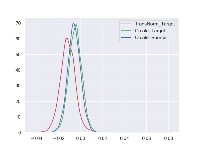
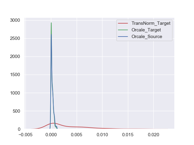
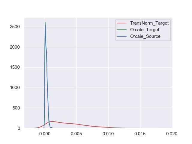
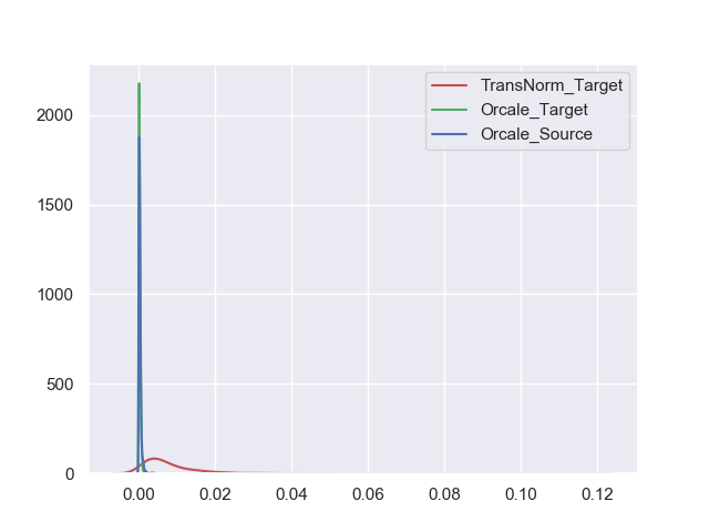
The batch normalization (BN) statistics are shown in Figure 9. We observe that in the Oracle source and target settings, the model has similar BN statistics in both mean and variance. This demonstrates that the gap between the source and target domains does not lie in the BNs, which is different from the conclusion in [47]. Hence, the modification of the BN statistics may have a negative effect, as in TransNorm[47], where the target BN statistics are far different from those of the Oracle target model. This observation is consistent with the results listed in Table 6. We speculate that the cause of this failure in the combined simulation dataset UDA experiments[44, 22, 47] is that the source and target domains have large spectral differences, and thus require domain-specific BN statistics. However, the LoveDA dataset is real data obtained from the same sensor at the same time. The spectral difference in the source and target domains is very small (Figure 3(b)), so the BN statistics are very similar (Figure 9).


A.7 Large-scale Visualizations on UDA Test Set
The large-scale visualizations are shown in the Figure 10. Compared with the baseline, CBST can produce better results on large-scale mapping, which highlights the importance of developing UDA methods. However, CBST still has a lot of room for improvement. More tailored UDA algorithms requires to be developed on the LoveDA dataset.