AE-StyleGAN: Improved Training of Style-Based Auto-Encoders

Abstract

StyleGANs have shown impressive results on data generation and manipulation in recent years, thanks to its disentangled style latent space. A lot of efforts have been made in inverting a pretrained generator, where an encoder is trained ad hoc after the generator is trained in a two-stage fashion. In this paper, we focus on style-based generators asking a scientific question: Does forcing such a generator to reconstruct real data lead to more disentangled latent space and make the inversion process from image to latent space easy? We describe a new methodology to train a style-based autoencoder where the encoder and generator are optimized end-to-end. We show that our proposed model consistently outperforms baselines in terms of image inversion and generation quality. Supplementary, code, and pretrained models are available on the project website.

1 Introduction

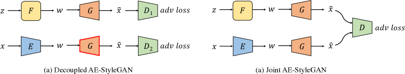
Figure 1: Model Architecture. (a) Decoupled AE-StyleGAN: $E$, $F$, $G$, $D$ are encoder, multi-layer perceptron, generator, and discriminator, respectively. We learn $E$ to map image space to $\mathcal{W}$ (or $\mathcal{W}^{+}$) space. The red outline around $G$ is to tell that in the encoder update step, generator is in gradient-freeze stage and only the encoder gets updated. (b) Joint AE-StyleGAN: Here, we train encoder along with generator at the same time with a shared discriminator. Please refer Algorithm 1 and Algorithm 2 for more details.

The generative adversarial networks (GAN) [11] in deep learning estimates how data points are generated in a probabilistic framework. It consists of two interacting neural networks: a generator, $G$, and a discriminator, $D$, which are trained jointly through an adversarial process. The objective of $G$ is to synthesize fake data that resemble real data, while the objective of $D$ is to distinguish between real and fake data. Through an adversarial training process, the generator can generate fake data that match the real data distribution. GANs have been applied to numerous tasks ranging from conditional image synthesis [25, 12, 15, 13], image translation [18, 41, 14, 27, 17], text-to-image generation [38, 32], image restoration [24, 26, 4] etc.

Most notably, StyleGANs [19, 20] propose a novel style-based generator architecture and attain state-of-the-art visual quality on high-resolution images. As it can effectively encode rich semantic information in the latent space [7, 34], we can edit the latent code and synthesize images with various attributes, such as aging, expression, and light direction. However, such manipulations in the latent space are only applicable to images generated from GANs rather than to any given real images due to the lack of inference functionality or the encoder in GANs.

In contrast, GAN inversion aims to invert a given image back into the latent space of a pretrained generator. The image can then be faithfully reconstructed from the inverted code by the generator. GAN inversion enables the controllable directions found in latent spaces of the existing trained GANs to be applicable to real image editing, without requiring ad-hoc supervision or expensive optimization. As StyleGAN is known to have a disentangled latent space which offers control and editing capabilities and has become common practice [2, 39, 1, 3] to encode real images into an extended latent space, $\mathcal{W}^{+}$, defined by the concatenation of ‘n’ different 512-dimensional $w$ vectors (or styles).

In this paper, we focus on a scientific question of how to train a style encoder along with a style-based generator. This essentially requires training a style-based autoencoder networks where the encoder and generator are optimized simultaneously end-to-end. This is different from GAN inversion literature where $G$ is fixed and autoencoding is implemented stage-wise. Adversarial Latent Autoencoders (or ALAE [30]) is one example to solve this problem, however, it often suffers from inferior generation quality (compared with original StyleGANs) and inaccurate reconstruction. We hypothesize that this is mainly because ALAE is trained to reconstruct fake images rather than real ones. Inspired by the success of in-domain GAN inversion [39], we propose a novel algorithm to train a style encoder jointly with StyleGAN generator to reconstruct real images during GAN training. We term our method AE-StyleGAN.

Another important aspect of autoencoders is their ability to learn disentangled representations. As stated in StyleGAN2 [20], a more disentangled generator is easier to invert. This motivates us to ask if its inverse proposition is also true. We thus interpret our AE-StyleGAN objective as a regularization and explore: whether enforcing the generator to reconstruct real data (easy to invert) leads to more disentangled latent space.

Finally, we list our contribution as follows: (1) We propose AE-StyleGAN as improved techniques for training style-based autoencoders; (2) We discovered that an easy-to-invert generator is also more disentangled; (3) AE-StyleGAN shows superior generation and reconstruction quality than baselines.

2 Related Works

GAN inversion. The AE-StyleGAN is closely related to GAN inversion methods. However, we aim to solve a different problem: GAN inversion [2, 1, 39, 5] aims at finding the most accurate latent code for the input image to reconstruct the input image with a pretrained and fixed GAN generator. While AE-StyleGAN aims to train an autoencoder-like structure where the encoder and generator are optimized end-to-end. There are two streams of GAN inversion approaches: (1) to optimize the latent codes directly [2, 1], or (2) to train an amortised encoder to predict the latent code given images [39, 5, 33, 37]. Notably, in-domain GAN inversion [39] proposes domain-guided encoder training that differs from traditional GAN inversion methods [40, 29] where encoders are trained with sampled image-latent pairs.

Learning a bidirectional GAN. There are two main approaches for learning a bidirectional GAN: (1) adversarial feature learning (BiGAN) [8] or adversarially learned inference (ALI) [9]; (2) combining autoencoder training with GANs, e.g. VAE/GAN [22], AEGAN [23]. We focus on the latter since it usually gives better reconstruction quality and its training is more stable [36]. Our AE-StyleGAN is different from these methods because these bidirectional models encode images in $\mathcal{Z}$ space (usually Gaussian) and are not designed for style-based generator networks.

Adversarial Latent Autoencoders. ALAE [30] is the most relevant work to ours. The proposed AE-StyleGAN is different from ALAE in that: (1) an ALAE discriminator is defined in latent space ($\mathcal{W}$) while ours is in image space; (2) ALAE reconstructs fake images by minimizing L2 between sampled $w$ and encoded fake image, while ours reconstruct real images.

3 Method

3.1 Background

GAN and StyleGAN. We denote image data as $\{x_{i}\}^{n}_{i=1}\subseteq\mathcal{X}$ drawn from the data distribution $P_{X}$. A generator is trained to transform samples $z\sim P_{Z}$ from a canonical distribution conditioned on labels to match the real data distributions. Real distributions are denoted as $P$ and generated distributions are denoted as $Q$. In this paper, we focus on StyleGANs and denote mapping network as $F:\mathcal{Z}\mapsto\mathcal{W}$, generator as $G:\mathcal{W}\mapsto\mathcal{X}$, and encoder as $E:\mathcal{X}\mapsto\mathcal{W}$ (or $\mathcal{W}^{+}$). We also denote fake and reconstructed images as $\tilde{x}=G(F(z))$ and $\hat{x}=G(E(x))$. The value function of GAN can be written as:

$$V_{\text{GAN}}(G\circ F,D)= -\mathbb{E}_{x\sim P_{X}}{\mathcal{A}(-\tilde{D}(x))}$$

$$-\mathbb{E}_{z\sim P_{Z}}{\mathcal{A}(\tilde{D}(G(F(z))))}$$ (1)

Here $\mathcal{A}$ is the activation function and $\tilde{D}$ is the logit or discriminator’s output before activation. Note that choosing $\mathcal{A}(t)=\text{softplus}(t)=\log{(1+\exp{(t)})}$ recovers the original GAN formulation [11, 19], and the resulting objective minimizes the Jensen-Shannon (JS) divergence between real and generated data distributions.

In-domain GAN inversion. In-domain GAN inversion [39] aims to learn a mapping from images to latent space. The encoder is trained to reconstruct real images (thus are “in-domain”) and guided by image-level loss terms, i.e. pixel MSE, VGG perceptual loss, and discriminator loss:

$$L_{\text{idinv}}(E,D,G)= \mathbb{E}_{x\sim P_{X}}[\|x-G(E(x))\|_{2}$$

$$+\lambda_{\text{vgg}}\|h(x)-h(G(E(x)))\|_{2}$$

$$-\lambda_{\text{adv}}\mathcal{A}({-\tilde{D}(G(E(x)))})],$$ (2)

where $h$ is perception network and here we keep the same as in-domain inversion as VGG network.

Negative data augmentation. NDA [35] produces out-of-distribution samples lacking the typical structure of natural images. NDA-GAN directly specifies what the generator should not generate through NDA distribution $\bar{P}$ and the resulting adversarial game is:

$$V_{\text{NDA}}(\lambda G\circ F+(1-\lambda)\bar{P},D)$$ (3)

where hyperparameter $\lambda$ is the mixture weight.

3.2 Auto-Encoding StyleGANs

Algorithm 1 Decoupled AE-StyleGAN Training

1:$\theta_{E},\theta_{D_{1}},\theta_{D_{2}},\theta_{F},\theta_{G}\leftarrow\text{Initialize network parameters}$

2:while not converged do

3:     $x\leftarrow\text{Random mini-batch from dataset}$

4:     $z\leftarrow\text{Samples from }\mathcal{N}(0,I)$

5:     Step I. Update $D_{1}$, $D_{2}$

6:     $L_{D}\leftarrow-V_{\text{GAN}}(G\circ F,D_{1})-V_{\text{GAN}}(G\circ E,D_{2})$ in 1

7:     $\theta_{D_{1}},\theta_{D_{2}}\leftarrow\text{ADAM}(\nabla_{\theta_{D_{1}},\theta_{D_{2}}}L_{D},\theta_{D_{1}},\theta_{D_{2}})$

8:     Step II. Update $E$

9:     $L_{E}\leftarrow L_{\text{idinv}}(E,{D_{2}},G)$ in 2 or 6

10:     $\theta_{E}\leftarrow\text{ADAM}(\nabla_{\theta_{E}}L_{E},\theta_{E})$

11:     Step III. Update $F$, $G$

12:     $L_{G}\leftarrow V_{\text{GAN}}(G\circ F,{D_{1}})$ in 1

13:     $\theta_{F},\theta_{G}\leftarrow\text{ADAM}(\nabla_{\theta_{F},\theta_{G}}L_{G},\theta_{F},\theta_{G})$

14:end while

Algorithm 2 Joint AE-StyleGAN Training

1:$\theta_{E},\theta_{D},\theta_{F},\theta_{G}\leftarrow\text{Initialize network parameters}$

2:while not converged do

3:     $x\leftarrow\text{Random mini-batch from dataset}$

4:     $z\leftarrow\text{Samples from }\mathcal{N}(0,I)$

5:     Step I. Update $D$

6:     $L_{D}\leftarrow-V_{\text{AEGAN}}(G\circ F,D)$ in 5

7:     $\theta_{D}\leftarrow\text{ADAM}(\nabla_{\theta_{D}}L_{D},\theta_{D})$

8:     Step II. Update $E$, $G$

9:     $L_{E}\leftarrow L_{\text{idinv}}(E,D,G)$ in 2 or 6

10:     $\theta_{E},\theta_{G}\leftarrow\text{ADAM}(\nabla_{\theta_{E},\theta_{G}}L_{E},\theta_{E},\theta_{G})$

11:     Step III. Update $F$, $G$

12:     $L_{G}\leftarrow V_{\text{AEGAN}}(G\circ F,D)$ in 5

13:     $\theta_{F},\theta_{G}\leftarrow\text{ADAM}(\nabla_{\theta_{F},\theta_{G}}L_{G},\theta_{F},\theta_{G})$

14:end while

Decoupled AE-StyleGAN. One straightforward way to train encoder and generator end-to-end is to simultaneously train an encoder with GAN inversion algorithms along with the generator. Here we choose in-domain inversion. To keep the generator’s generating ability intact, one can decouple GAN training and GAN inversion training by introducing separate discriminator models $D_{1}$ and $D_{2}$, and freezing $G$ in inversion step. Specifically, $D_{1}$ is involved in $V_{\text{GAN}}(G\circ F,D_{1})$ in Equation 1 for GAN training steps, and $D_{2}$ is involved in $L_{\text{idinv}}(E,D_{2},G)$ in Equation 2. Training of $D_{2}$ follows:

$$V_{\text{GAN}}(G\circ F,D_{2})= -\mathbb{E}_{x\sim P_{X}}{\mathcal{A}(-\tilde{D}_{2}(x))}$$

$$-\mathbb{E}_{x\sim P_{X}}{\mathcal{A}(\tilde{D}_{2}(G(E(x))))}.$$ (4)

Please refer to Figure 1-a and Algorithm 1 for details.

It is worth mentioning that this decoupled algorithm is similar to CR-GAN [36] except that we use decoupled discriminators.

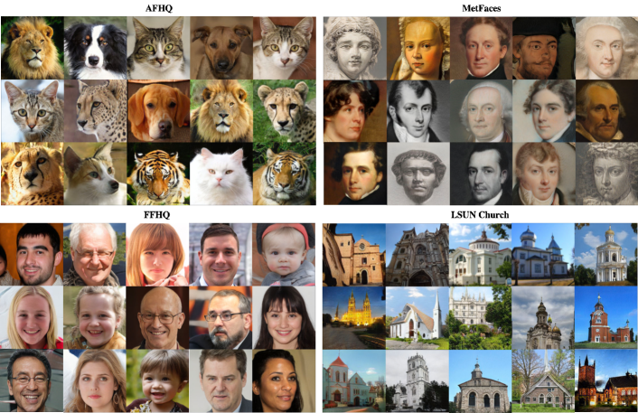
Figure 2: Generations with AE-StyleGAN ($\mathcal{W}^{+}$). The model generates lot of diverse images which is justified by its LPIPS score tabulated in Table 1.

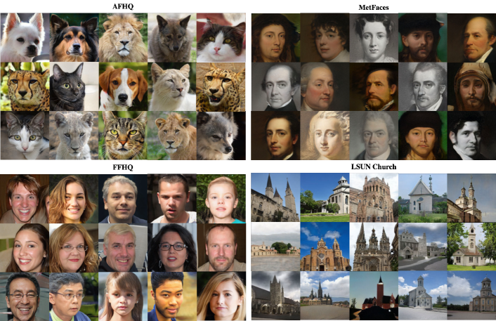
Figure 3: Generations with ALAE. Although, these are comparable in quality, AE-StyleGAN ($\mathcal{W}^{+}$) still outperforms ALAE by huge margin Table 1

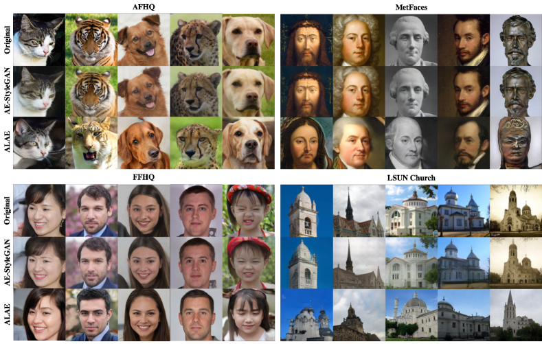
Figure 4: Reconstructions with AE-StyleGAN ($\mathcal{W}^{+}$) and ALAE. AE-StyleGAN not only reconstructs the main objects but also preserves details like background, color, expression, etc. While reconstructions with ALAE suffer with identity loss. For example, the Dog and Tiger images from AFHQ in this grid are reconstructed with modified expression, face shape, color.

Joint AE-StyleGAN. The generator of a decoupled AE-StyleGAN would be exactly equivalent to a standard StyleGAN generator, however, we often find the encoder not capable of faithfully reconstruct real images. This phenomenon is illustrated in Figure 5. We hypothesize that with $G$ frozen at inversion step, $E$ cannot catch up with $G$’s update, thus lags behind $G$. To cope with this issue, we propose to train $G$ jointly with $E$ in the inversion step. We also use a single discriminator for both pathways. For the GAN pathway, the value function is written as:

$$V_{\text{AEGAN}}(G\circ F,D)= -\mathbb{E}_{x\sim P_{X}}{\mathcal{A}(-\tilde{D}(x))}$$ (5)

$$-\lambda_{\text{adv}}\mathbb{E}_{x\sim P_{X}}{\mathcal{A}(\tilde{D}(G(E(x))))}$$

$$-(1-\lambda_{\text{adv}})\mathbb{E}_{z\sim P_{Z}}{\mathcal{A}(\tilde{D}(G(F(z))))}.$$

This can be viewed as a differentiable NDA, with $\bar{P}$ set to be the distribution of reconstructed real images, and $\lambda=1-\lambda_{\text{adv}}$. Please refer to Figure 1-b and Algorithm 2 for details. In the following text, we use AE-StyleGAN to refer Joint AE-StyleGAN, if not explicitly specified.

Adaptive discriminator weight. Inspired by VQGAN [10], we also experimented with adding an adaptive weight to automatically balance reconstruction loss and adversarial loss:

$$L^{\text{ada}}_{\text{idinv}}= L_{\text{rec}}+\beta L_{\text{adv}},$$

$$\text{where}~{}~{}L_{\text{rec}}= \mathbb{E}_{x\sim P_{X}}[\|x-G(E(x))\|_{2}$$

$$+\lambda_{\text{vgg}}\|h(x)-h(G(E(x)))\|_{2}],$$

$$\text{and}~{}~{}L_{\text{adv}}= -\lambda_{\text{adv}}\mathbb{E}_{x\sim P_{X}}[\mathcal{A}({-\tilde{D}(G(E(x)))})],$$

$$\text{with}\quad~{}~{}\beta= \frac{\nabla_{\theta^{l}_{G}}[L_{\text{rec}}]}{\nabla_{\theta^{l}_{G}}[L_{\text{adv}}]+\epsilon},$$ (6)

where $L_{\text{rec}}$ is the weighted sum of pixel reconstruction loss and VGG perceptual loss, $\nabla_{\theta^{l}_{G}}[\cdot]$ is the gradient of its input w.r.t. the last layer $l$ of generator, and $\epsilon=10^{-6}$ added for numerical stability. In the following text, we use AE-StyleGAN with adaptive $\beta$ for all experiments if not specified.

Table 1: Fréchet Inception Distances (FID), and the Learned Perceptual Image Patch Similarity (LPIPS) are computed for all the models over all datasets. Our proposed Joint AE-StyleGAN achieves the lowest FID and highest LPIPS in most cases. The top-two best performing methods are marked in boldface.

	StyleGAN		ALAE		AE-StyleGAN ($\mathcal{W}$)		AE-StyleGAN ($\mathcal{W}^{+}$)
	FID $\downarrow$	LPIPS $\uparrow$	FID $\downarrow$	LPIPS $\uparrow$	FID $\downarrow$	LPIPS $\uparrow$	FID $\downarrow$	LPIPS $\uparrow$
FFHQ	7.359	0.432	12.574	0.438	8.176	0.448	7.941	0.451
AFHQ	7.992	0.496	21.557	0.508	15.655	0.522	10.282	0.518
MetFaces	29.318	0.465	41.693	0.462	29.710	0.469	29.041	0.471
LSUN Church	27.780	0.520	29.999	0.552	29.387	0.603	29.358	0.592

Table 2: PPL. Perceptual path lengths on FFHQ, AFHQ, MetFaces and Church dataset are computed on all models over all datasets (lower is better). Our model is performing 13% to 20% better than ALAE on complex datasets like LSUN church and FFHQ. The top-two best performing methods are marked in boldface.

	StyleGAN		ALAE		AE-StyleGAN ($\mathcal{W}$)		AE-StyleGAN ($\mathcal{W}^{+}$)
	Full	End	Full	End	Full	End	Full	End
FFHQ	173.09	173.68	192.60	193.94	181.03	180.23	166.70	165.85
AFHQ	244.83	240.68	229.54	232.53	247.75	248.75	233.86	231.91
MetFaces	231.40	232.77	235.39	237.63	238.84	238.60	240.01	235.41
LSUN Church	245.22	239.62	298.06	295.01	241.46	231.73	240.01	231.49

Table 3: Reconstruction VGG, Per Pixel MSE and FID comparison. VGG perceptual loss, Pixel MSE and FID values are computed between real images and their reconstructions for ALAE, Joint AE-StyleGAN ($\mathcal{W}$) & Joint AE-StyleGAN ($\mathcal{W}^{+}$). The best performing methods are marked in boldface.

	ALAE			AE-StyleGAN ($\mathcal{W}$)			AE-StyleGAN ($\mathcal{W}^{+}$)
	VGG $\downarrow$	MSE $\downarrow$	FID $\downarrow$	VGG$\downarrow$	MSE $\downarrow$	FID $\downarrow$	VGG $\downarrow$	MSE $\downarrow$	FID $\downarrow$
FFHQ	0.81	64.82	21.68	0.28	26.10	16.76	0.26	25.34	14.67
AFHQ	0.99	73.77	25.30	0.29	29.21	5.37	0.27	28.75	4.90
MetFaces	0.54	49.72	52.55	0.05	13.48	27.38	0.05	13.34	25.34
LSUN Church	0.86	76.97	43.52	0.30	32.29	26.45	0.29	31.75	32.67

4 Experiments

Datasets. We evaluate AE-StyleGAN with four datasets: (1) FFHQ dataset which consists of 70,000 images of people faces aligned and cropped at resolution of $1024\times 1024$; (2) AFHQ dataset consisting of 15,000 images from domains of cat, dog, and wildlife; (3) MetFaces dataset consists of 1,336 high-quality human face images at $1024\times 1024$ resolution collected from art works in the Metropolitan Museum; (4) The LSUN Churches contains 126,000 outdoor photographs of churches of diverse architectural styles. For a fair comparison, we resized all images to $128\times 128$ resolution for training.

Baselines. We compare our proposed models with ALAE as a competitive baseline. For a fair comparison, we implemented ALAE following the paper [31], Joint AE-StyleGAN, Decoupled AE-StyleGAN on the same backbone StyleGAN2.

Evaluation metrics. Fréchet Inception Distances (FID) [16], learned perceptual image patch similarity (LPIPS), Perceptual Path Length (PPL) and are reported for quantitative evaluation in Table 1 and Table 2. Experimental setup and additional results are detailed in Appendix.

4.1 Implementation

The code is written in PyTorch [28] and heavily based on Rosinality’s implementation of StyleGAN2 [20]. For image encoders, we modify the last linear layer of the image discriminator to desired dimensions, and remove its mini-batch standard deviation layer. We keep the default values for hyperparameters of in-domain inversion and fix $\lambda_{\text{vgg}}=5\times 10^{-5}$ and $\lambda_{\text{adv}}=0.1$ for all experiments. For a fair comparison, we reimplemented ALAE under the same codebase.

4.2 Qualitative Analysis

Decoupled vs. Joint AE-StyleGAN. We also compare Decoupled AE-StyleGAN with Joint AE-StyleGAN with a visualization of real image reconstruction as the training progresses. From Figure 5, especially for a complex dataset like FFHQ, we see a lot of noise, artifacts in the reconstructions of Decoupled AE-StyleGAN which can be explained with the fact that the encoder is not being trained jointly with generator, hence it is failing to cope up with generator’s learning curve thus compromising on the reconstruction quality. However, as the encoder is being trained jointly with generator in Joint AE-StyleGAN, it does not lag behind generator which helps it to faithfully reconstruct the real image. Another interesting observation to support this argument is that the Decoupled AE-StyleGAN’s encoder is performing much better on AFHQ data which is a simple dataset when compared with FFHQ. However, we can observe strong facial deformation and Jointly trained encoder in Joint AE-StyleGAN is able to reconstruct it well unanimously. This analysis also adds strong weight on our claim that training an encoder jointly with generator helps in finding a more disentangled latent space thus, reinforcing a better real image reconstruction capability.

ALAE vs. Joint AE-StyleGAN. We compare Joint AE-StyleGAN with ALAE through sampled images and real image reconstructions. From Figure 2 and Figure 3 we can observe that the sample image generation quality of ALAE is comparable to Joint AE-StyleGAN qualitatively (Joint AE-StyleGAN still outperforms ALAE in terms of FID and LPIPS by a large margin, see Table 1). However, ALAE fails to reconstruct a real image accurately, where the reconstruction looses its identity from the original image which is very evident from Figure 4. On the other hand, Joint AE-StyleGAN does not only reconstruct a real image faithfully but also preserves details like background, color, expression, etc. outperforming ALAE as shown in Figure 4.

Style transfer. We also experimented with style transfer as shown in Figure 6 between real images from FFHQ to support our claim that Joint AE-StyleGAN’s training algorithm in fact creates a more disentangled $\mathcal{W}$ (or $\mathcal{W}^{+}$) space. We use an encoder trained via Joint AE-StyleGAN ($\mathcal{W}^{+}$) method and pass 11 real images that are randomly chosen from FFHQ dataset to the encoder to obtain $\mathcal{W}^{+}$ latent codes. As we are working with $128\times 128$ resolution images, our $\mathcal{W}^{+}$ latent code consists of 12 styles latent vectors, each of size 512. We experimented with various combinations of these latent vectors from source B to source A and found that mixing 7 to 11 style latents from source B’s $\mathcal{W}^{+}$ latent code to source A’s $\mathcal{W}^{+}$ latent code gave us meaningful style transfer results. Thus proving our argument that Joint AE-StyleGAN training methodology in fact helps in creating a more disentangled $\mathcal{W}$ (or $\mathcal{W}^{+}$) space and helps in real image editing.

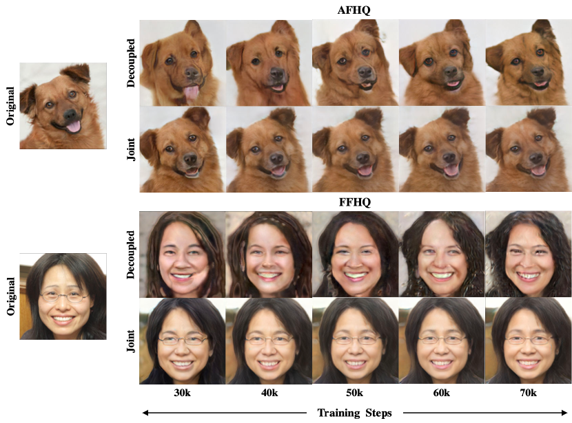
Figure 5: Reconstruction progress for AFHQ and FFHQ for Decoupled and Joint AE-StyleGAN. Decoupled model’s reconstructions are with noise, artifacts, identity loss. Joint AE-StyleGAN faithfully reconstructs the image as the training progresses.

4.3 Quantitative Analysis

We did a quantitative comparison of ALAE, AE-StyleGAN ($\mathcal{W}$), AE-StyleGAN ($\mathcal{W}^{+}$) and StyleGAN2 by computing FID, LPIPS. First, to be on the common ground, we use the same implementation of StyleGAN2 to serve as a backbone for ALAE and AE-StyleGAN. Upon optimising these models over four datasets FFHQ, AFHQ, MetFaces and LSUN Church we are reporting FID and LPIPS scores through Table 1. Our model surpassed ALAE in terms of FID and LPIPS in all datasets. To strengthen the evidence, we also did PPL computations on every model for all the datasets. It is interesting to note from Table 2 that our model beats ALAE in most cases. Especially, for complex datasets like FFHQ and LSUN Church, PPL scores of AE-StyleGAN is 13% to 22% better than those of ALAE. Although PPL scores of ALAE for simpler datasets like AFHQ ahd MetFaces is comparable, our model still outperforms ALAE. At last, we compared VGG loss (or perceptual loss), Pixel loss, FID of real images and reconstructed images for all the best models and tabulated them at Table 3. We can also see that Joint AE-StyleGAN outperforms ALAE in terms of inverting the generator with an observed VGG, MSE losses more than 50% less than ALAE.

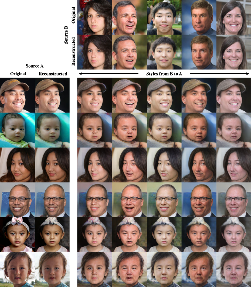
Figure 6: Style transfer within FFHQ. Style transfer experiment between two sets of real images from FFHQ dataset. We reconstruct real images via Joint AE-StyleGAN $\mathcal{W}^{+}$ and use $\mathcal{W}^{+}$ latent codes of all the images and copy specified subset of styles from source B to source A, thus creating an image grid as above that show original images and their reconstructions as well as the style mixed images from source B to source A

4.4 Ablation Study

In our early experiments, we ablate hyperparameters including whether to use decoupled discriminators, whether to jointly update $G$, and the number of $E$ step per $G$ step on VoxCeleb2 dataset [6] at resolution $64\times 64$. Sample FID and per pixel reconstruction MSE are reported in Table 4. We can observe that if $G$ is not jointly updated with $E$, the reconstruction MSE only decreases slightly even with 4 $E$-steps. While jointly updating $G$ improves MSE substantially.

Table 4: Ablation studies. Decouple $D$: whether to use decoupled discriminators; Joint $G$: whether to jointly update $G$; $\#$ $E$-step: number of $E$ step per $G$ step. All metrics are evaluated at 20000 iterations.

Decouple $D$	Joint $G$	$\#$ $E$-step	FID $\downarrow$	MSE $\downarrow$
✓	✗	1	36.101	13.716
✓	✗	4	34.632	12.202
✓	✓	1	35.384	8.701
✓	✓	4	35.409	5.872
✗	✗	1	39.611	13.229
✗	✗	4	37.559	12.822
✗	✓	1	35.048	8.454
✗	✓	4	36.602	5.924

Table 5: Adaptive discriminator weight. Comparing sample FID and reconstruction MSE evaluated on FFHQ dataset. With adaptive weight $\beta$, generator achieves better FID and MSE.

	AE-StyleGAN ($\mathcal{W}$)		AE-StyleGAN ($\mathcal{W}^{+}$)
	w/o $\beta$	w/ $\beta$	w/o $\beta$	w/ $\beta$
FID $\downarrow$	8.620	8.177	8.241	7.941
MSE $\downarrow$	30.683	26.107	29.726	25.341

We also ablate adaptive discriminator weight defined in Equation 6 on FFHQ at $128\times 128$ resolution. Sample FID and per pixel reconstruction MSE are reported in Table 5. We can observe that using adaptive weight consistently improves both FID and MSE metrics.

5 Conclusion

In this paper, we proposed AE-StyleGAN, a novel algorithm that jointly trains an encoder with a style-based generator. With empirical analysis, we confirmed that this methodology provides an easy-to-invert encoder for real image editing. Extensive results showed that our model has superior image generation and reconstruction capability than baselines. We have explored the problem of training an end-to-end autoencoder. With improved generation fidelity and reconstruction quality, the proposed AE-StyleGAN model can serve as a building-block for further development and applications. For example, it could potentially improve CR-GAN [36] where an encoder is involved in generator training. It also enables further improvement of disentanglement by borrowing techniques such as Factor-VAE [21]. We leave these for future work.

References

- [1] Rameen Abdal, Yipeng Qin, and Peter Wonka. Image2stylegan++: How to edit the embedded images? CoRR, abs/1911.11544, 2019.
- [2] Rameen Abdal, Yipeng Qin, and Peter Wonka. Image2stylegan: How to embed images into the stylegan latent space?, 2019.
- [3] Rameen Abdal, Peihao Zhu, Niloy J. Mitra, and Peter Wonka. Styleflow: Attribute-conditioned exploration of stylegan-generated images using conditional continuous normalizing flows. CoRR, abs/2008.02401, 2020.
- [4] Mahmoud Afifi, Marcus A Brubaker, and Michael S Brown. Histogan: Controlling colors of gan-generated and real images via color histograms. In Proceedings of the IEEE/CVF Conference on Computer Vision and Pattern Recognition, pages 7941–7950, 2021.
- [5] Yuval Alaluf, Or Patashnik, and Daniel Cohen-Or. Restyle: A residual-based stylegan encoder via iterative refinement. In Proceedings of the IEEE/CVF International Conference on Computer Vision, pages 6711–6720, 2021.
- [6] Joon Son Chung, Arsha Nagrani, and Andrew Zisserman. Voxceleb2: Deep speaker recognition. arXiv preprint arXiv:1806.05622, 2018.
- [7] Edo Collins, Raja Bala, Bob Price, and Sabine Süsstrunk. Editing in style: Uncovering the local semantics of gans. CoRR, abs/2004.14367, 2020.
- [8] Jeff Donahue, Philipp Krähenbühl, and Trevor Darrell. Adversarial feature learning. arXiv preprint arXiv:1605.09782, 2016.
- [9] Vincent Dumoulin, Ishmael Belghazi, Ben Poole, Olivier Mastropietro, Alex Lamb, Martin Arjovsky, and Aaron Courville. Adversarially learned inference. arXiv preprint arXiv:1606.00704, 2016.
- [10] Patrick Esser, Robin Rombach, and Bjorn Ommer. Taming transformers for high-resolution image synthesis. In Proceedings of the IEEE/CVF Conference on Computer Vision and Pattern Recognition, pages 12873–12883, 2021.
- [11] Ian Goodfellow, Jean Pouget-Abadie, Mehdi Mirza, Bing Xu, David Warde-Farley, Sherjil Ozair, Aaron Courville, and Yoshua Bengio. Generative adversarial nets. In Advances in neural information processing systems, pages 2672–2680, 2014.
- [12] Ligong Han, Ruijiang Gao, Mun Kim, Xin Tao, Bo Liu, and Dimitris Metaxas. Robust conditional gan from uncertainty-aware pairwise comparisons. In Proceedings of the AAAI Conference on Artificial Intelligence, volume 34, pages 10909–10916, 2020.
- [13] Ligong Han, Martin Renqiang Min, Anastasis Stathopoulos, Yu Tian, Ruijiang Gao, Asim Kadav, and Dimitris N. Metaxas. Dual projection generative adversarial networks for conditional image generation. In Proceedings of the IEEE/CVF International Conference on Computer Vision (ICCV), pages 14438–14447, October 2021.
- [14] Ligong Han, Robert F Murphy, and Deva Ramanan. Learning generative models of tissue organization with supervised gans. In 2018 IEEE Winter Conference on Applications of Computer Vision (WACV), pages 682–690. IEEE, 2018.
- [15] Ligong Han, Anastasis Stathopoulos, Tao Xue, and Dimitris Metaxas. Unbiased auxiliary classifier gans with mine. arXiv preprint arXiv:2006.07567, 2020.
- [16] Martin Heusel, Hubert Ramsauer, Thomas Unterthiner, Bernhard Nessler, and Sepp Hochreiter. Gans trained by a two time-scale update rule converge to a local nash equilibrium. In Advances in neural information processing systems, pages 6626–6637, 2017.
- [17] Xun Huang, Ming-Yu Liu, Serge J. Belongie, and Jan Kautz. Multimodal unsupervised image-to-image translation. CoRR, abs/1804.04732, 2018.
- [18] Phillip Isola, Jun-Yan Zhu, Tinghui Zhou, and Alexei A Efros. Image-to-image translation with conditional adversarial networks. In Proceedings of the IEEE conference on computer vision and pattern recognition, pages 1125–1134, 2017.
- [19] Tero Karras, Samuli Laine, and Timo Aila. A style-based generator architecture for generative adversarial networks. In Proceedings of the IEEE/CVF Conference on Computer Vision and Pattern Recognition, pages 4401–4410, 2019.
- [20] Tero Karras, Samuli Laine, Miika Aittala, Janne Hellsten, Jaakko Lehtinen, and Timo Aila. Analyzing and improving the image quality of stylegan. In Proceedings of the IEEE/CVF Conference on Computer Vision and Pattern Recognition, pages 8110–8119, 2020.
- [21] Hyunjik Kim and Andriy Mnih. Disentangling by factorising. In International Conference on Machine Learning, pages 2649–2658. PMLR, 2018.
- [22] Anders Boesen Lindbo Larsen, Søren Kaae Sønderby, Hugo Larochelle, and Ole Winther. Autoencoding beyond pixels using a learned similarity metric. In International conference on machine learning, pages 1558–1566. PMLR, 2016.
- [23] Conor Lazarou. Autoencoding generative adversarial networks. arXiv preprint arXiv:2004.05472, 2020.
- [24] Christian Ledig, Lucas Theis, Ferenc Huszár, Jose Caballero, Andrew Cunningham, Alejandro Acosta, Andrew Aitken, Alykhan Tejani, Johannes Totz, Zehan Wang, et al. Photo-realistic single image super-resolution using a generative adversarial network. In Proceedings of the IEEE conference on computer vision and pattern recognition, pages 4681–4690, 2017.
- [25] Mehdi Mirza and Simon Osindero. Conditional generative adversarial nets. arXiv preprint arXiv:1411.1784, 2014.
- [26] Kamyar Nazeri, Eric Ng, and Mehran Ebrahimi. Image colorization using generative adversarial networks. In International conference on articulated motion and deformable objects, pages 85–94. Springer, 2018.
- [27] Taesung Park, Ming-Yu Liu, Ting-Chun Wang, and Jun-Yan Zhu. Semantic image synthesis with spatially-adaptive normalization. In Proceedings of the IEEE/CVF Conference on Computer Vision and Pattern Recognition, pages 2337–2346, 2019.
- [28] Adam Paszke, Sam Gross, Francisco Massa, Adam Lerer, James Bradbury, Gregory Chanan, Trevor Killeen, Zeming Lin, Natalia Gimelshein, Luca Antiga, et al. Pytorch: An imperative style, high-performance deep learning library. In Advances in neural information processing systems, pages 8026–8037, 2019.
- [29] Guim Perarnau, Joost van de Weijer, Bogdan Raducanu, and Jose M. Álvarez. Invertible conditional gans for image editing. CoRR, abs/1611.06355, 2016.
- [30] Stanislav Pidhorskyi, Donald A Adjeroh, and Gianfranco Doretto. Adversarial latent autoencoders. In Proceedings of the IEEE/CVF Conference on Computer Vision and Pattern Recognition, pages 14104–14113, 2020.
- [31] Stanislav Pidhorskyi, Donald A. Adjeroh, and Gianfranco Doretto. Adversarial latent autoencoders. CoRR, abs/2004.04467, 2020.
- [32] Scott Reed, Zeynep Akata, Xinchen Yan, Lajanugen Logeswaran, Bernt Schiele, and Honglak Lee. Generative adversarial text to image synthesis. arXiv preprint arXiv:1605.05396, 2016.
- [33] Elad Richardson, Yuval Alaluf, Or Patashnik, Yotam Nitzan, Yaniv Azar, Stav Shapiro, and Daniel Cohen-Or. Encoding in style: a stylegan encoder for image-to-image translation. In Proceedings of the IEEE/CVF Conference on Computer Vision and Pattern Recognition, pages 2287–2296, 2021.
- [34] Yujun Shen, Jinjin Gu, Xiaoou Tang, and Bolei Zhou. Interpreting the latent space of gans for semantic face editing. CoRR, abs/1907.10786, 2019.
- [35] Abhishek Sinha, Kumar Ayush, Jiaming Song, Burak Uzkent, Hongxia Jin, and Stefano Ermon. Negative data augmentation. arXiv preprint arXiv:2102.05113, 2021.
- [36] Yu Tian, Xi Peng, Long Zhao, Shaoting Zhang, and Dimitris N Metaxas. Cr-gan: learning complete representations for multi-view generation. arXiv preprint arXiv:1806.11191, 2018.
- [37] Omer Tov, Yuval Alaluf, Yotam Nitzan, Or Patashnik, and Daniel Cohen-Or. Designing an encoder for stylegan image manipulation. ACM Transactions on Graphics (TOG), 40(4):1–14, 2021.
- [38] Han Zhang, Tao Xu, and Hongsheng Li. Stackgan: Text to photo-realistic image synthesis with stacked generative adversarial networks. 2017 IEEE International Conference on Computer Vision (ICCV), pages 5908–5916, 2016.
- [39] Jiapeng Zhu, Yujun Shen, Deli Zhao, and Bolei Zhou. In-domain gan inversion for real image editing. In European conference on computer vision, pages 592–608. Springer, 2020.
- [40] Jiapeng Zhu, Deli Zhao, and Bo Zhang. LIA: latently invertible autoencoder with adversarial learning. CoRR, abs/1906.08090, 2019.
- [41] Jun-Yan Zhu, Taesung Park, Phillip Isola, and Alexei A Efros. Unpaired image-to-image translation using cycle-consistent adversarial networks. In Proceedings of the IEEE international conference on computer vision, pages 2223–2232, 2017.