Multifractal of mass function

Abstract

Multifractal plays an important role in many fields. However, there is few attentions about mass function, which can better deal with uncertain information than probability. In this paper, we proposed multifractal of mass function. Firstly, the definition of multifractal spectrum of mass function is given. Secondly, the multifractal dimension of mass function is defined as $D_{\alpha}$. When mass function degenerates to probability distribution, $D_{\alpha}$ degenerates to $d_{\alpha}$, which is information dimension proposed by Renyi. One interesting property is that the multifractal dimension of mass function with maximum Deng entropy is 1.585 no matter the order. Other interesting properties and numerical examples are shown to illustrate proposed model.

1 Introduction

In recently years, much research has focus on fractal theory [1, 2] since many natural phenomenon [3, 4] and system [5, 6] can be characterized by the fractal properties. Thus, fractal plays a vital role in many fields such as mechanical engineering [7, 8], geotechnical engineering [9, 10, 11], oscillator model [12, 13], molecular structure [14, 15] and so on. Lots of models about fractal dimension are proposed [16, 17], which is the main parameter of measuring irregular objects. To better analyse the property of fractal, many models about multifractal [18, 19, 20] were proposed, which as a generalization of fractal can better describe the variation of local features. For example, the characteristics of multifractal spectrum was analysed to study the stability of the China’s stock market [21]. A generalization of classical multifractal detrended fluctuation analysis was proposed by Wang [22]. A method named multifractal cross wavelet analysis was developed to characterizes the properties of complex system [23].

How to deal with uncertain information has attracted a lot of attention [24, 25, 26]. Many models like probability theory [27, 28], fuzzy sets [29, 30, 31], evidence theory [32, 33, 34], rough sets [35, 36] are developed. Mass function is a significant component of evidence theory [37, 38] and has an advantage over probability distribution in dealing with uncertainty problem [39]. Lots of parameters of mass function were studied like divergence [40], correlation coefficient [41, 42], distance [43, 44]. In addition, the uncertainty of mass function has been studied extensively [45, 46]. The negation of mass function was developed by Gao [47] and Mao [48]. Some effective combination rule of conflict mass function were proposed [49, 50, 51]. Transform mass function into probability is still a hot topic [52, 53]. However, there is few attentions paid to mass function from the perspective of multifractal. In this paper, the multifractal analysis of mass function are given including multifractal spectrum and multifractal dimension.

This article is organized as follows. Section 2 is a brief introduction about preliminaries. Multifractal spectrum of mass function is showed in Section 3. In Section 4, the definition of multifractal dimension is given. Detailed calculation and numerical examples are following. Finally is a simple conclusion for whole work.

2 Preliminaries

2.1 Multifractal spectrum

Consider a measure space $(\chi,B(\chi),\mu)$. There is a lattice covering of $\chi$ by $d-$dimensional boxes of width $\delta_{n}$, where $B_{\delta_{n}}(x)$ is the box that contains the point $x$ [54]. $U_{n}(x)$ is function with the condition $\delta_{n}\rightarrow 0$ as $n\rightarrow\infty$ [54].

$$U_{n}(x)=-log\mu\left[B_{\delta_{n}}(x)\right],\ if\ \mu\left[B_{\delta_{n}}(x)\right]>0\,.$$ (1)

Let $Y_{n}(x)$ be a rescaled version of $U_{n}(x)$ with the condition $\lim_{n\rightarrow\infty}Pr\left\{Y_{n}=y\right\}=0$ if $y\neq y_{0}$ [54].

$$Y_{n}(x)=\frac{U_{n}(x)}{-log\delta_{n}}\,.$$ (2)

The multifractal spectrum is defined as follows [54].

$$\widetilde{f}(y)=\lim_{n\rightarrow\infty}\frac{logN_{n}}{-log\delta_{n}}+\lim_{\epsilon\rightarrow 0}\lim_{n\rightarrow 0}\frac{Pr\left\{|Y_{n}-y|<\epsilon\right\}}{-log\delta_{n}}\,.$$ (3)

Where $N_{n}$ is the number of boxes at the $n$th stage with positive $\mu$ measure [54]. The first term is the box counting dimension of the support of $\mu$ and the second term is the rate of the probability function $Y_{n}$ approaches zeros [54].

2.2 Renyi entropy and Renyi information dimension

2.2.1 Renyi entropy

Entropy is an important measure in many fields [55, 56]. A classic entropy named Renyi entropy is defined as follows [57].

Consider a probability distribution $P_{X}$ of a discrete random variable $X$: $P_{X}=\left\{p_{i}|i=1,2,...,n\right\}$, its Renyi entropy is,

$$H_{\alpha}(P)=\frac{1}{1-\alpha}log\sum_{i}^{n}p_{i}^{\alpha}\,.$$ (4)

Where $\alpha\geq 0$. When $\alpha\rightarrow 1$, Renyi entropy degenerates to Shannon entropy [58].

$$\lim_{\alpha\rightarrow 1}H_{\alpha}(P)=\sum_{i}^{n}p_{i}logp_{i}=H_{S}\,.$$ (5)

2.2.2 Renyi information dimension

The dimension of the probability distribution of $X$ defined by Renyi is as follows [59].

$$d_{\alpha}=\lim_{n\rightarrow\infty}\frac{H_{\alpha}(P)}{log_{2}n}\,.$$ (6)

When $\alpha\rightarrow 1$, $d_{\alpha}$ represents the rate of Shannon entropy grows with scale.

2.3 Mass function

Mass function assigns mass on power set and its definition is as follows.

Let $\Theta$ is the framework of discernment in evidence theory [37, 38],

$$\Theta=\{\theta_{1},\cdots,\theta_{n}\},n\in N^{+}\,.$$ (7)

Its power set is,

$$\begin{split}2^{\Theta}=&\{A_{1},\ A_{2},...,\ A_{2^{n}}\}\\ =&\{\{\theta_{1}\},\cdots,\ \{\theta_{1},\theta_{2}\},\cdots,\ \{\Theta\},\ \emptyset\},\,.\end{split}$$ (8)

Mass function is a mapping $m:2^{\Theta}\rightarrow[0,1]$ satisfing [37, 38],

$$m(\emptyset)=0,\,$$ (9)

$$\quad\sum_{A_{i}\in 2^{\Theta}}m(A_{i})=1\,.$$ (10)

where $A_{i}$ is called focal element when $m(A_{i})>0$.

2.4 Deng entropy

Given a framework of discernment is $\Theta$ and a mass function is $m(A_{i})$. Deng entropy is defined as follows [60].

$$H_{D}=-\sum_{A_{i}\in 2^{\Theta}}m(A_{i})log(\frac{m(A_{i})}{2^{|A_{i}|}-1})\,.$$ (11)

Where $|A_{i}|$ is the cardinal of focal element. When mass function satisfies the condition,

$$m(A_{i})=\frac{2^{|A_{i}|}-1}{\sum_{i}2^{|A_{i}|}-1},\,$$ (12)

Deng entropy reaches the maximum [60].

$$H_{maxD}=-\sum_{i}m(A_{i})log(\frac{m(A_{i})}{2^{|A_{i}|}-1})=log\sum_{i}({2^{|A_{i}|}-1})\,.$$ (13)

Deng entropy considers the non-specificity of mass function and is studied widely [61, 62, 63].

3 Multifractal spectrum of mass function

We first generalizes the concept of multifractal spectrum of mass function, then some examples are shown to illustrate the proposed model.

Definition 3.1.

A measure space in evidence theory is $(\Theta,2^{\Theta},m)$. Where $m$ is a mass function of $2^{\Theta}$. The multifractal spectrum is defined as follows.

$$\widetilde{f}(y)=\frac{log_{2}N_{n}}{-log_{2}(2^{|\Theta|}-1)^{-1}}\,.$$ (14)

Where $N_{n}$ is the number of focal elements that have the same mass and $y$ is calculated as follows.

$$y(A_{i})=\frac{-log_{2}m(A_{i})}{-log_{2}(2^{|\Theta|}-1)^{-1}}\,.$$ (15)

$y$ can be explained as the rate at which mass function changes with respect to the size of $\Theta$. $\widetilde{f(y)}$ is a function of $y$ and following is a detailed process.

Example 1: Consider a framework of discernment is $\Theta=\left\{\theta_{1},\theta_{2},\theta_{3}\right\}$. A mass function assignment with maximum Deng entropy is $m(\theta_{1})=m(\theta_{2})=m(\theta_{3})=1/19$, $m(\theta_{1},\theta_{2})=m(\theta_{1},\theta_{3})=m(\theta_{2},\theta_{3})=3/19$, $m(\theta_{1},\theta_{2},\theta_{3})=7/19$. According to Eq. (14) and Eq. (15)

$$y(\theta_{1})=y(\theta_{2})=y(\theta_{3})=\frac{-log_{2}(1/19)}{-log_{2}(2^{3}-1)^{-1}}=1.5131\,.$$ (16)

$$y(\theta_{1},\theta_{2})=y(\theta_{1},\theta_{3})=y(\theta_{2},\theta_{3})=\frac{-log_{2}(3/19)}{-log_{2}(2^{3}-1)^{-1}}=0.9486\,.$$ (17)

$$y(\theta_{1},\theta_{2},\theta_{3})=\frac{-log_{2}(1/19)}{-log_{2}(2^{3}-1)^{-1}}=0.5131\,.$$ (18)

$$\widetilde{f}(y(\theta_{1}))=\widetilde{f}(y(\theta_{2}))=\widetilde{f}(y(\theta_{3}))=\frac{log_{2}(3)}{-log_{2}(2^{3}-1)^{-1}}=0.5646\,.$$ (19)

$$\widetilde{f}(y(\theta_{1},\theta_{2}))=\widetilde{f}(y(\theta_{1},\theta_{3}))=\widetilde{f}(y(\theta_{2},\theta_{3}))=\frac{log_{2}(3)}{-log_{2}(2^{3}-1)^{-1}}=0.5646\,.$$ (20)

$$\widetilde{f}(y(\theta_{1},\theta_{2},\theta_{3}))=\frac{log_{2}(1)}{-log_{2}(2^{3}-1)^{-1}}=0\,.$$ (21)

From above calculations, if the cardinal of the focal elements is equal, their mass functions are the same and have the same $y$. These pairs of points are drawn in Fig. 1.

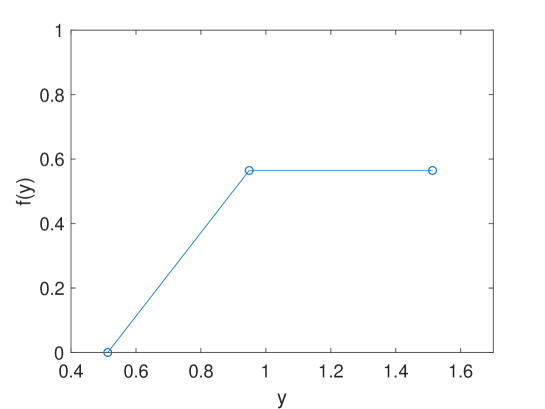
Figure 1: The multifractal spectrum of Example 1

Example 2: Consider a framework of discernment is $\Theta$, $|\Theta|=2,...,n$. A series of mass functions assigned with maximum Deng entropy are $m_{i}$, $i=2,...,n$. The multifractal spectrums are shown in Fig. 2. and Fig. 3. Part of the values of $y$ and $\widetilde{f}(y)$ are shown in Table 1 and Table 2.

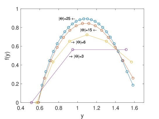
Figure 2: The multifractal spectrum of Example 2 when $|\Theta|=3,6,15,25$

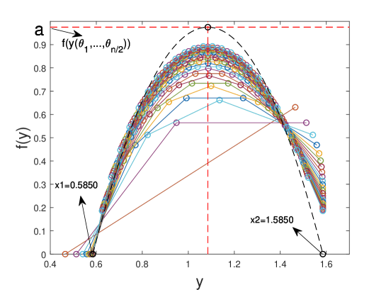
Figure 3: The multifractal spectrum of Example 2 with $|\Theta|=1,...,25$

The value of $y$ with the increase of $|\Theta|$ of Example 2. $y(\theta_{1})$ $y(\theta_{1},\theta_{2})$ $y(\theta_{1},...,\theta_{3})$ $y(\theta_{1},...,\theta_{4})$ $y(\theta_{1},...,\theta_{5})$ $y(\theta_{1},...,\theta_{6})$ $...$ $|\Theta|=2$00 01.4650 00.4650 $|\Theta|=3$00 01.5131 00.9486 00.5131 $|\Theta|=4$00 01.5415 01.1358 00.8229 00.5415 $|\Theta|=5$00 01.5585 01.2386 00.9918 00.7699 00.5585 $|\Theta|=6$00 01.5688 01.3036 01.0991 00.9152 00.7400 00.5688

The value of $\widetilde{f}(y)$ with the increase of $|\Theta|$ of Example 2. $\widetilde{f}(y(\theta_{1}))$ $\widetilde{f}(y(\theta_{1},\theta_{2}))$ $\widetilde{f}(y(\theta_{1},...,\theta_{3}))$ $\widetilde{f}(y(\theta_{1},...,\theta_{4}))$ $\widetilde{f}(y(\theta_{1},...,\theta_{5}))$ $\widetilde{f}(y(\theta_{1},...,\theta_{6}))$ $...$ $|\Theta|=2$00 00.6309 00 $|\Theta|=3$00 00.5646 00.5646 00 $|\Theta|=4$00 00.5119 00.6616 00.5119 00 $|\Theta|=5$00 00.4687 00.6705 00.6705 00.4687 00 $|\Theta|=6$00 00.4325 00.6536 00.7231 00.6536 00.4325 00

As can be seen from Fig. 3, the multifractal spectrum in this example is plotted by solid colored lines. The black dotted line is the case that $\lim_{|\Theta|\rightarrow\infty}$. In other words, the multifractal spectrum of of mass function with maximum Deng entropy when $n\rightarrow\infty$ can be approximated by a quadratic function $F(x)=-a(x-0.585)(x-1.585)$, where $a=\frac{4log_{2}C_{n}^{\frac{n}{2}}}{n}$. Proof is as follows. According to Eq. (12), Eq. (14) and Eq. (15).

$$\lim_{n\rightarrow\infty}m(\theta_{1})=\frac{2^{1}-1}{C_{n}^{1}(2^{1}-1)+C_{n}^{2}(2^{2}-1)+...+C_{n}^{n}(2^{n}-1)}=\frac{1}{3^{n}-2^{n}}\,.$$ (22)

$$\lim_{n\rightarrow\infty}m(\theta_{1},...,\theta_{\frac{n}{2}})=\frac{2^{\frac{n}{2}}-1}{C_{n}^{1}(2^{1}-1)+C_{n}^{2}(2^{2}-1)+...+C_{n}^{n}(2^{n}-1)}=\frac{2^{\frac{n}{2}}-1}{3^{n}-2^{n}}\,.$$ (23)

$$\lim_{n\rightarrow\infty}m(\theta_{1},...,\theta_{n})=\frac{2^{n}-1}{C_{n}^{1}(2^{1}-1)+C_{n}^{2}(2^{2}-1)+...+C_{n}^{n}(2^{n}-1)}=\frac{2^{n}-1}{3^{n}-2^{n}}\,.$$ (24)

$$\begin{split}\lim_{n\rightarrow\infty}y(\theta_{1})=\frac{-log_{2}(3^{n}-2^{n})^{-1}}{-log_{2}(2^{n}-1)^{-1}}=\frac{log_{2}(2^{n})+log_{2}(\frac{3}{2}^{n}-1)}{log_{2}(2^{n}-1)}\approx 1.5850\,.\end{split}$$ (25)

$$\lim_{n\rightarrow\infty}y(\theta_{1},...,\theta_{\frac{n}{2}})=\frac{-log_{2}(\frac{2^{\frac{n}{2}}-1}{3^{n}-2^{n}})}{-log_{2}(2^{n}-1)^{-1}}=\frac{-log_{2}(2^{\frac{n}{2}})+log_{2}(\frac{3}{2}^{n}-1)}{log_{2}(2^{n}-1)}\approx 1.0850\,.$$ (26)

$$\lim_{n\rightarrow\infty}y(\theta_{1},...,\theta_{n})=\frac{-log_{2}(\frac{2^{n}-1}{3^{n}-2^{n}})}{-log_{2}(2^{n}-1)^{-1}}=0.5850\,.$$ (27)

$$\lim_{n\rightarrow\infty}\widetilde{f}(y(\theta_{1})=\frac{log_{2}(C_{n}^{1})}{-log_{2}(2^{n}-1)^{-1}}\approx\frac{log_{2}(n)}{n}\approx 0\,.$$ (28)

$$\lim_{n\rightarrow\infty}\widetilde{f}(y(\theta_{1},...,\theta_{\frac{n}{2}}))=\frac{log_{2}(C_{n}^{\frac{n}{2}})}{-log_{2}(2^{n}-1)^{-1}}=\approx\frac{log_{2}(C_{n}^{\frac{n}{2}})}{n}\,.$$ (29)

$$\lim_{n\rightarrow\infty}\widetilde{f}(y(\theta_{1},...,\theta_{n}))=\frac{log_{2}(C_{n}^{n})}{-log_{2}(2^{n}-1)^{-1}}\approx\frac{log_{2}(1)}{n}=0\,.$$ (30)

$$\left\{(y(\theta_{1}),\widetilde{f}(y(\theta_{1}))),(1.5850,0)\right\}$$

$$\left\{(y(\theta_{1},...,\theta_{n}),\widetilde{f}(y(\theta_{1},\theta_{n}))),(0.5850,0)\right\}$$

There are three points $(0.5850,0)$, $(1.0850,\frac{log_{2}(C_{n}^{\frac{n}{2}})}{n})$, $(1.5850,0)$, thus the quadratic function is calculated as $F(x)=-a(x-0.585)(x-1.585)$, where $a=\frac{4log_{2}C_{n}^{\frac{n}{2}}}{n}$.

Example 3: Consider a framework of discernment is $\Theta$, $|\Theta|=2,...,n$. A mass function averagely assigned on $2^{\Theta}$ is $m_{i}(A)=\frac{1}{2^{|\Theta|}-1}$, $i=2,...,n$. The multifractal spectrums is only one point $(1,1)$ in Fig. 4.

$$y(\theta_{1})=...=y(\theta_{1},\theta_{2})=...=y(\theta_{1},...,\theta_{n})=\frac{-log_{2}(2^{n}-1)^{-1}}{-log_{2}(2^{n}-1)^{-1}}=1\,.$$ (31)

$$\widetilde{f}(y(\theta_{1}))=...=\widetilde{f}(y(\theta_{1},...,\theta_{n}))=\frac{log_{2}(2^{n}-1)}{-log_{2}(2^{n}-1)^{-1}}=1\,.$$ (32)

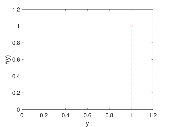
Figure 4: The multifractal spectrum of Example 3 with $|\Theta|=1,...,25$

Example 4: Consider a framework of discernment is $\Theta$, $|\Theta|=2,...,n$. A mass function is $m_{i}(\Theta)=1$, $i=2,...,n$. The multifractal spectrums is only one point $(0,0)$ in Fig. 5.

$$y(\Theta)=\frac{-log_{2}(1)^{-1}}{-log_{2}(2^{n}-1)^{-1}}=0\,.$$ (33)

$$\widetilde{f}(y(\Theta))=\frac{log_{2}(1)}{-log_{2}(2^{n}-1)^{-1}}=0\,.$$ (34)

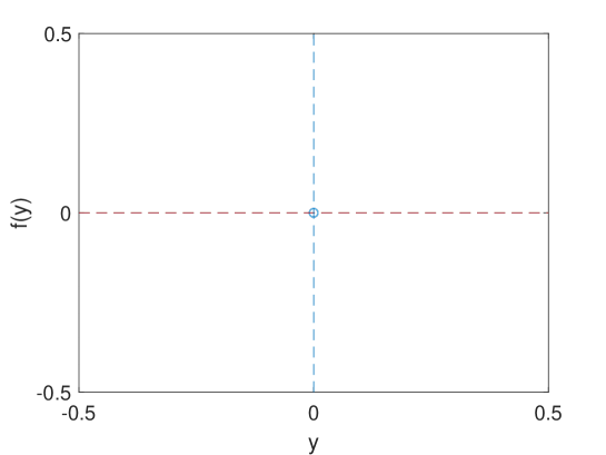
Figure 5: The multifractal spectrum of Example 4 with $|\Theta|=1,...,25$

4 Multifractal dimension of mass function

Definition 4.1.

The multifractal dimension of mass function is defined as follows.

$$D_{\alpha}(m(A_{i}))=\frac{\frac{1}{1-\alpha}log_{2}\left[\sum_{i}(\frac{m(A_{i})}{2^{|A_{i}|}-1|})^{\alpha}(2^{|A_{i}|}-1)\right]}{log_{2}\sum_{i}(2^{|A_{i}|}-1)^{m(A_{i})^{\alpha}}}\,.$$ (35)

Theorem 4.2.

$\lim_{\alpha\rightarrow 1}D_{\alpha}(m(A_{i}))=\frac{-\sum_{i}m(A_{i})log_{2}(\frac{m(A_{i})}{2^{|A_{i}|}-1})}{log_{2}\sum_{i}(2^{|A_{i}|}-1)^{m(A_{i})}}$, where the numerator is Deng entropy.

Proof 4.3.

$$\begin{split}\lim_{\alpha\rightarrow 1}D_{\alpha}(m(A_{i}))=&\lim_{\alpha\rightarrow 1}\frac{\frac{\partial}{\partial\alpha}\left[log_{2}\sum_{i}(\frac{m(A_{i})}{2^{|A_{i}|}-1|})^{\alpha}(2^{|A_{i}|}-1)\right]}{\frac{\partial}{\partial\alpha}\left[(1-\alpha)(log_{2}\sum_{i}(2^{|A_{i}|}-1)^{m(A_{i})^{\alpha}})\right]}\\ =&\frac{\sum_{i}\left[(\frac{m(A_{i})}{2^{|A_{i}|}-1|})^{\alpha}(2^{|A_{i}|}-1)log_{2}(\frac{m(A_{i})}{2^{|A_{i}|}-1})\right]}{(-log_{2}\sum_{i}(2^{|A_{i}|}-1)^{m(A_{i})^{\alpha}})+(1-\alpha)T}\\ =&\frac{-\sum_{i}m(A_{i})log_{2}(\frac{m(A_{i})}{2^{|A_{i}|}-1})}{log_{2}\sum_{i}(2^{|A_{i}|}-1)^{m(A_{i})}}\,.\end{split}$$ (36)

Where $T$ is $\left[log_{2}\sum_{i}(2^{|A_{i}|}-1)^{m(A_{i})^{\alpha}}\right]^{{}^{\prime}}$, which multipled by $(1-\alpha)$ tend to be 0 when $\alpha\rightarrow 1$.

Theorem 4.4.

When mass function degenerates to probability distribution, the proposed multifractal dimension degenerates to Renyi information dimension.

Proof 4.5.

$$\begin{split}D_{\alpha}(m_{i}\rightarrow P_{i})=&\frac{\frac{1}{1-\alpha}log_{2}\left[\sum_{i}(\frac{p_{i}}{2^{1}-1})^{\alpha}(2^{1}-1)\right]}{log_{2}\sum_{i}(2^{1}-1)^{p_{i}^{\alpha}}}\\ =&\frac{\frac{1}{1-\alpha}log_{2}\sum_{i}p_{i}^{\alpha}}{log_{2}n}\\ =&d_{\alpha}\,.\end{split}$$ (37)

Theorem 4.6.

Let $\Theta$ has $n$ elements, a mass function with maximum Deng entropy is $m(A_{i})=\frac{2^{|A_{i}|-1}}{\sum_{i}2^{|A_{i}|}-1}$, $\lim_{n\rightarrow\infty}D_{\alpha}=1.585$, where $\alpha\in R$.

Proof 4.7.

$$\begin{split}\lim_{n\rightarrow\infty}D_{\alpha}(m(A_{i}))=&\frac{\frac{1}{1-\alpha}log_{2}\left[\sum_{i}(\frac{\frac{2^{|A_{i}|}-1}{\sum_{i}(2^{|A_{i}|}-1)}}{2^{|A_{i}|}-1|})^{\alpha}(2^{|A_{i}|}-1)\right]}{log_{2}\sum_{i}(2^{|A_{i}|}-1)^{\frac{2^{|A_{i}|}-1}{\sum_{i}(2^{|A_{i}|}-1)}^{\alpha}}}\\ =&\frac{\frac{1}{1-\alpha}log_{2}(3^{n}-2^{n})^{-\alpha}(\sum_{i}2^{|A_{i}|}-1)}{log_{2}(2^{|\Theta|}-1)}\\ =&\frac{\frac{1}{1-\alpha}log_{2}(3^{n}-2^{n})^{1-\alpha}}{log_{2}2^{n}}\\ \approx&1.585\,.\end{split}$$ (38)

Where $\lim_{n\rightarrow\infty}(2^{|A_{i}|}-1)^{\frac{2^{|A_{i}|}-1}{\sum_{i}(2^{|A_{i}|}-1)}^{\alpha}}=(2^{|A_{i}|}-1)^{(\frac{2^{|A_{i}|}-1}{3^{n}-2^{n}})^{\alpha}}\approx((2^{|A_{i}|}-1)^{0})^{\alpha}=1$ and there are $(2^{|\Theta|}-1)$ terms.

Theorem 4.8.

Let $\Theta$ has $n$ elements, a mass function is $m(\theta_{i})=\frac{1}{|\Theta|}=\frac{1}{n}$, $i=1,2,...,n$. $\lim_{n\rightarrow\infty}D_{\alpha}=1$, where $\alpha\in R$.

Proof 4.9.

$$\begin{split}\lim_{n\rightarrow\infty}D_{\alpha}(m(A_{i}))=&\frac{\frac{1}{1-\alpha}log_{2}\sum_{i}(\frac{n^{-1}}{2^{|\theta_{i}|}-1|})^{\alpha}(2^{|\theta_{i}|}-1)}{log_{2}\sum_{i}(2^{|\theta_{i}|}-1)^{(n^{-1})^{\alpha}}}\\ =&\frac{\frac{1}{1-\alpha}log_{2}\sum_{i}({n^{-1}})^{\alpha}}{log_{2}\sum_{i}^{n}(1)}\\ =&\frac{\frac{1}{1-\alpha}log_{2}n^{1-\alpha}}{log_{2}n}\\ =&1\,.\end{split}$$ (39)

It should be noted that in this theorem, mass function degenerates to probability and the proposed multifractal dimension degenerates to Renyi information dimension. This theorem can be written as: the Renyi information dimension of uniform distribution is a fixed point 1 no matter what $\alpha$ is.  

Example 5: Given a framework of discernment is $\Theta=\left\{\theta_{1},\theta_{2},\theta_{3}\right\}$. A mass function is $m(\theta_{1})=0.2,\ m(\theta_{2},\theta_{3})=0.8$. The results of multifractal dimension are shown in Table 3. The detailed calculations are as follows.

When $\alpha=1$, according to Theorem 1,

$$D_{\alpha}=\frac{-(0.2\times log_{2}(\frac{0.2}{2^{1}-1})+0.8\times log_{2}(\frac{0.8}{2^{2}-1}))}{log_{2}((2^{1}-1)^{0.2}+(2^{2}-1)^{0.8})}=1.1249\,.$$ (40)

When $\alpha=2$,

$$D_{\alpha}=\frac{-\frac{1}{1-2}\times log_{2}\left[(\frac{0.2}{2^{1}-1})^{2}\times(2^{1}-1)+(\frac{0.8}{2^{2}-1})^{2}\times(2^{2}-1)\right]}{log_{2}\left[((2^{1}-1)^{0.2})^{2}+((2^{2}-1)^{0.8})^{2}\right]}=0.7163\,.$$ (41)

The result of Example 5. $\alpha=3$ $\alpha=9$ $\alpha=15$ $\alpha=21$ $\alpha=27$ $\alpha=33$ $...$ $D_{\alpha}$00 00.5759 00.2390 00.1472 00.1060 00.0828 00.0679

As can be seen from Table 3, $D_{\alpha}$ goes to zero as $\alpha$ increasing.

Example 6: Given a framework of discernment is $\Theta$, $|\Theta|=2,...,n$. A mass function is $m_{i}(\Theta)=1$, $i=2,...,n$. The results are show in Table 4 and Fig. 6. Detailed calculations are as follows.

$$\begin{split}D_{\alpha}=&\frac{\frac{1}{1-\alpha}log_{2}(\frac{m(\Theta)}{2^{|\Theta|}-1})^{\alpha}(2^{|\Theta|}-1)}{log_{2}\left[(2^{|\Theta|}-1)^{m(\Theta)}\right]^{\alpha}}\\ =&\frac{\frac{1}{1-\alpha}log_{2}(\frac{1}{2^{n}-1})^{\alpha-1}}{log_{2}\left[(2^{n}-1)^{1}\right]^{\alpha}}\\ =&\frac{log_{2}(2^{n}-1)}{\alpha log_{2}(2^{n}-1)}\\ =&\frac{1}{\alpha}\,.\end{split}$$ (42)

From Eq. (42), the multifractal dimensions of $m(\Theta)=1$ are only related to the order $\alpha$ and as $\alpha$ increases, $D_{\alpha}$ decreases.

The result of Example 6. $|\Theta|=n$ $\setminus$ $\alpha$ $1$ $4$ $7$ $10$ $13$ $16$ $19$ $D_{\alpha}$00 01 00.25 00.1429 00.1 00.0769 00.0625 00.0526

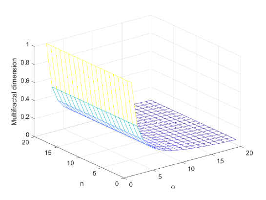
Figure 6: The change of multifractal dimension of Example 6

Example 7: Given a framework of discernment is $\Theta$, $|\Theta|=2,...,n$. A mass function is $m(\theta_{i})=\frac{1}{|\Theta|}$. The result is calculated as follows.

$$d_{\alpha}=\frac{\frac{1}{1-\alpha}log_{2}\sum_{i}^{n}(\frac{1}{n})^{\alpha}}{log_{2}n}=\frac{log_{2}n}{log_{2}n}=1\,.$$ (43)

In this example, the mass function degenerates to probability distribution. According to Theorem 2, the proposed dimension degenerates to Renyi information dimension. From Eq. (43), the multifractal dimension of $m(\theta_{i})=\frac{1}{n}$ is 1. It doesn’t depend on $\alpha$ and $n$. This example illustrates Theorem 4.

Example 8: Given a framework of discernment is $\Theta$, $|\Theta|=2,...,n$. A mass function is $m(A_{i})=\frac{1}{2^{|\Theta|}-1)}$. The results are shown in Table 5 and Fig. 7.

The result of Example 8. $|\Theta|$ $\setminus$ $\alpha$ $1$ $5$ $9$ $13$ $17$ $21$ $25$ $29$ $2$00 01.1850 00.5682 00.3413 00.2370 00.1804 00.1455 00.1218 00.1048 $4$00 01.3811 00.9707 00.8180 00.7146 00.6321 00.5637 00.5061 00.4462 $6$00 01.4520 01.0988 01.0023 00.9518 00.9138 00.8814 00.8521 00.8251 $8$00 01.4798 01.1433 01.0599 01.0265 01.0062 00.9911 00.9787 00.9679 $10$00 01.4911 01.1620 01.0788 01.0491 01.0333 01.0230 01.0156 01.0097 $12$00 01.4959 01.1724 01.0865 01.0568 01.0417 01.0324 01.0261 01.0215 $14$00 01.4981 01.1795 01.0907 01.0603 01.0450 01.0357 01.0296 01.0251 $16$00 01.4991 01.1851 01.0973 01.0624 01.0467 01.0373 01.0311 01.0266 $18$00 01.4995 01.1897 01.0960 01.0640 01.0480 01.0384 01.0320 01.0264 $20$00 01.4998 01.1935 01.0980 01.0653 01.0490 01.0392 01.0327 01.0280

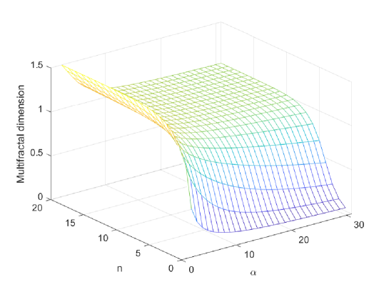
Figure 7: The change of multifractal dimension of Example 8

As can be seen from Table 5, the multifractal dimension is getting closer and closer to 1 when the size of framework of discernment bigger with higher order $\alpha$. This rule of change can be seen more intuitively in Fig. 7. Actually, we can come to this conclusion directly from the definition as follows.

$$\begin{split}\lim_{n\rightarrow\infty,\alpha\rightarrow\infty}D_{G\alpha}=&\frac{\frac{1}{1-\alpha}log_{2}\left[\sum_{i}(\frac{\frac{1}{2^{n}-1}}{2^{|A_{i}|}-1|})^{\alpha}(2^{|A_{i}|}-1)\right]}{log_{2}\sum_{i}(2^{|A_{i}|}-1)^{(\frac{1}{2^{n}-1})^{\alpha}}}\\ \approx&\frac{\frac{1}{1-\alpha}log_{2}\sum_{i}^{2^{n}-1}(\frac{1}{2^{n}-1})^{\alpha}}{log_{2}\sum_{i}^{2^{n}-1}(1)^{\alpha}}\\ \approx&\frac{\frac{1}{1-\alpha}log_{2}(2^{n}-1)^{1-\alpha}}{log_{2}(2^{n}-1)}\\ =&1\,.\end{split}$$ (44)

Example 9: Given a framework of discernment is $\Theta$, $|\Theta|=2,...,n$. A mass function with maximum Deng entropy is $m(A_{i})=\frac{2^{|A_{i}|}-1}{\sum_{i}(2^{|A_{i}|}-1)}$. The multifractal dimensions are shown in Table 6 and Fig. 8.

The result of Example 9. $|\Theta|$ $\setminus$ $\alpha$ $1$ $4$ $7$ $10$ $13$ $16$ $19$ $2$00 01.1752 00.5809 00.3473 00.2441 00.1878 00.1526 00.1285 $4$00 01.4699 01.1962 00.8893 00.6589 00.5124 00.4172 00.3515 $6$00 01.5516 01.4904 01.4065 01.2899 01.1437 00.9919 00.8575 $8$00 01.5747 01.5611 01.5457 01.5275 01.5052 01.4770 01.4406 $10$00 01.5816 01.5784 01.5750 01.5715 01.5677 01.5637 01.5593 $12$00 01.5838 01.5830 01.5822 01.5814 01.5806 01.5797 01.5789 $14$00 01.5846 01.5844 01.5842 01.5840 01.5838 01.5836 01.5834 $16$00 01.5848 01.5848 01.5847 01.5847 01.5846 01.5846 01.5845 $18$00 01.5849 01.5849 01.5849 01.5849 01.5849 01.5848 01.5848 $20$00 01.5849 01.5849 01.5849 01.5849 01.5849 01.5849 01.5849

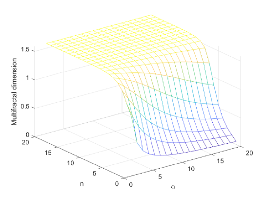
Figure 8: The change of multifractal dimension of Example 9

It can be seen from Table 6 and Fig. 8 that when the order $\alpha$ is determined, the multifractal dimension increases and finally tends to a constant with the increase of the framework of discernment. When the size of $|\Theta|$ is determined, the multifractal dimension decreases with the improvement of $\alpha$. More specifically, when the size of the framework of discernment is small, the multifractal dimension will decrease to 0 finally. When $n$ get bigger, the tendency to decrease gets smaller and smaller until it doesn’t change and remains $1.5850$. This example demonstrates Theorem 3.

5 Conclusion

In this paper, the multifractal spectrum of mass function is defined. Three special assignments are studied. The multifractal spectrum of mass function with maximum Deng entropy approximates quadratic function $F=-a(x-0.585)(x-1.585)$, where $a=\frac{4log_{2}C_{n}^{\frac{n}{2}}}{n}$. The multifractal spectrum of mass function with total uncertainty is the point (0,0) and with average assignment on power set is the point (1,1). Another important work is that we propose multifractal dimension of mass function. It noted that when mass function degenerates to probability and is distributed averagely, the proposed dimension degenerates to Renyi information dimension and is a constant 1. In addition, the multifractal dimension of mass function with maximum Deng entropy goes to 1.585 with the condition $\alpha\rightarrow\infty,\ |\Theta|\rightarrow\infty$. Other interesting properties are discussed. The changes of proposed dimension with differnet parameters $\alpha$ and the size of the framework of discernment $\Theta$ are shown by numerical examples.

References

- [1] Mandelbrot and B. Benoit, “The fractal geometry of nature”, American Journal of Physics 51 (1998) 468 p.
- [2] C. L. Kiew, A. Brahmananda, K. T. Islam, H. N. Lee, S. A. Venier, A. Saraar and H. Namazi, “Analysis of the relation between fractal structures of machined surface and machine vibration signal in turning operation”, Fractals 28 (2020) 2050019.
- [3] H. Yu, X. Liu, B. Kong, R. Li and G. Wang, “Landscape ecology development supported by geospatial technologies: A review”, Ecological Informatics 51 (2019) 185–192.
- [4] L. Liu, S. Li, X. Li, Y. Jiang, W. Wei, Z. Wang and Y. Bai, “An integrated approach for landslide susceptibility mapping by considering spatial correlation and fractal distribution of clustered landslide data”, Landslides 16 (2019) 715–728.
- [5] A. Harabagiu, O. Niculescu, M. Colotin, T. D. Bibire, I. Gottlieb and M. Agop, “Particle in a box by means of a fractal hydrodynamic model”, Romanian Reports in Physics 61 (2009) 395–400.
- [6] H. Namazi, A. Daneshi, H. Azarnoush, S. Jafari and F. Towhidkhah, “Fractal-based analysis of the influence of auditory stimuli on eye movements”, Fractals 26 (2018) 1850040.
- [7] H. Zhao and Q. Wu, “Application study of fractal theory in mechanical transmission”, Chinese Journal of Mechanical Engineering 29 (2016) 871–879.
- [8] G. Fang, X. Chang, P. Zhang and L. Wei, “Simulation calculation of temperature of the end face for mechanical seals based on fractal theory”, in Journal of Physics: Conference Series (IOP Publishing, 2019), volume 1168, p. 052060.
- [9] B. Li, R. Bao, Y. Wang, R. Liu and C. Zhao, “Permeability evolution of two-dimensional fracture networks during shear under constant normal stiffness boundary conditions”, Rock Mechanics and Rock Engineering 54 (2021) 409–428.
- [10] L. Li, W. Wu, M. H. El Naggar, G. Mei and R. Liang, “Characterization of a jointed rock mass based on fractal geometry theory”, Bulletin of Engineering Geology and the Environment 78 (2019) 6101–6110.
- [11] R. Guo, T. Nian, P. Li, J. Fu and H. Guo, “Anti-erosion performance of asphalt pavement with a sub-base of cement-treated mixtures”, Construction and Building Materials 223 (2019) 278–287.
- [12] K.-L. Wang, “A new fractal transform frequency formulation for fractal nonlinear oscillators”, Fractals 29 (2021) 2150062–1251.
- [13] A. Elías-Zúñiga, L. M. Palacios-Pineda, I. H. Jiménez-Cedeño, O. Martínez-Romero and D. O. Trejo, “Equivalent power-form representation of the fractal toda oscillator”, Fractals 29 (2021) 2150034–115.
- [14] M. K. Siddiqui, M. Imran and M. A. Iqbal, “Molecular descriptors of discrete dynamical system in fractal and cayley tree type dendrimers”, Journal of Applied Mathematics and Computing 61 (2019) 57–72.
- [15] J. Ding, M. Asta and R. O. Ritchie, “On the question of fractal packing structure in metallic glasses”, Proceedings of the National Academy of Sciences 114 (2017) 8458–8463.
- [16] T. Wen and K. H. Cheong, “The fractal dimension of complex networks: A review”, Information Fusion 73 (2021) 87–102.
- [17] A. Gires, I. Tchiguirinskaia, D. Schertzer, S. Ochoa-Rodriguez, P. Willems, A. Ichiba, L.-P. Wang, R. Pina, J. V. Assel, G. Bruni et al., “Fractal analysis of urban catchments and their representation in semi-distributed models: imperviousness and sewer system”, Hydrology and Earth System Sciences 21 (2017) 2361–2375.
- [18] R. Lopes and N. Betrouni, “Fractal and multifractal analysis: a review”, Medical image analysis 13 (2009) 634–649.
- [19] F. Landais, F. Schmidt and S. Lovejoy, “Multifractal topography of several planetary bodies in the solar system”, Icarus 319 (2019) 14–20.
- [20] S. Sanyal, A. Banerjee, S. Nag, U. Sarkar, S. Roy, R. Sengupta and D. Ghosh, “Tagore and neuroscience: A non-linear multifractal study to encapsulate the evolution of tagore songs over a century”, Entertainment Computing 37 (2021) 100367.
- [21] Y. Li, A. L. Vilela and H. E. Stanley, “The institutional characteristics of multifractal spectrum of china’s stock market”, Physica A: Statistical Mechanics and its Applications 550 (2020) 124129.
- [22] J. Wang and W. Shao, “Multifractal analysis with detrending weighted average algorithm of historical volatility”, Fractals 29 (2021) 2150193–114.
- [23] Z.-Q. Jiang, X.-L. Gao, W.-X. Zhou and H. E. Stanley, “Multifractal cross wavelet analysis”, Fractals 25 (2017) 1750054.
- [24] C. Wang, Z. X. Tan, Y. Ye, L. Wang, K. H. Cheong and N.-g. Xie, “A rumor spreading model based on information entropy”, Scientific reports 7 (2017) 1–14.
- [25] Y. Xue and Y. Deng, “Tsallis extropy”, Communications in Statistics-Theory and Methods (2021) 10.1080/03610926.2021.1921804.
- [26] K. H. Cheong, J. M. Koh and M. C. Jones, “Paradoxical survival: Examining the parrondo effect across biology”, BioEssays 41 (2019) 1900027.
- [27] X. Liu, W. Zhang, X. Gu and Z. Ye, “Probability distribution model of stress impact factor for corrosion pits of high-strength prestressing wires”, Engineering Structures 230 (2021) 111686.
- [28] W. Jiang, C. Huang and X. Deng, “A new probability transformation method based on a correlation coefficient of belief functions”, International Journal of Intelligent Systems 34 (2019) 1337–1347.
- [29] T. Senapati and R. R. Yager, “Fermatean fuzzy sets”, Journal of Ambient Intelligence and Humanized Computing 11 (2020) 663–674.
- [30] F. Kutlu Gündoğdu and C. Kahraman, “Spherical fuzzy sets and spherical fuzzy topsis method”, Journal of intelligent & fuzzy systems 36 (2019) 337–352.
- [31] F. Xiao, “CaFtR: A fuzzy complex event processing method”, International Journal of Fuzzy Systems (2021) DOI: 10.1007/s40815–021–01118–6.
- [32] F. Xiao, “CEQD: A complex mass function to predict interference effects”, IEEE Transactions on Cybernetics (2021) DOI: 10.1109/TCYB.2020.3040770.
- [33] Y. Deng, “Information volume of mass function”, International Journal of Computers Communications & Control 15 (2020) 3983.
- [34] L. Zhou, H. Cui, H. Huang, B. Kang and J. Zhang, “Counter deception in belief functions using shapley value methodology”, International Journal of Fuzzy Systems (2021) DOI:10.1007/s40815–021–01139–1.
- [35] R. Yan, Z. Wu and Q. Han, “A short note on rough set over dual-universes”, Journal of Experimental & Theoretical Artificial Intelligence 30 (2018) 725–731.
- [36] J. C. R. Alcantud, F. Feng and R. R. Yager, “An -soft set approach to rough sets”, IEEE Transactions on Fuzzy Systems 28 (2019) 2996–3007.
- [37] A. P. Dempster, “Upper and lower probabilities induced by a multivalued mapping”, The annals of mathematical statistics (1967) 325–339.
- [38] G. Shafer, A mathematical theory of evidence, volume 42 (Princeton university press, 1976).
- [39] D. Chen and H. Xie, “Fire safety evaluation for scenic spots: An evidential best-worst method”, Journal of Mathematics 2021 (2021) https://doi.org/10.1155/2021/5592150.
- [40] H. Wang, X. Deng, W. Jiang and J. Geng, “A new belief divergence measure for dempster–shafer theory based on belief and plausibility function and its application in multi-source data fusion”, Engineering Applications of Artificial Intelligence 97 (2021) 104030.
- [41] W. Jiang, “A correlation coefficient for belief functions”, International Journal of Approximate Reasoning 103 (2018) 94–106.
- [42] C. Qiang and Y. Deng, “A new correlation coefficient of mass function in evidence theoty and its application in fault diagnosis.”, Applied Intelligence 21 (2021) 10.1007/s10489–021–02797–2.
- [43] F. Xiao, “Ced: A distance for complex mass functions”, IEEE transactions on neural networks and learning systems 32 (2020) 1525–1535.
- [44] D. Han, J. Dezert and Y. Yang, “Belief interval-based distance measures in the theory of belief functions”, IEEE Transactions on Systems, Man, and Cybernetics: Systems 48 (2016) 833–850.
- [45] Y. Xue and Y. Deng, “Interval-valued belief entropies for Dempster Shafer structures”, Soft Computing 25 (2021) 8063–8071.
- [46] M. Khalaj, R. Tavakkoli-Moghaddam, F. Khalaj and A. Siadat, “New definition of the cross entropy based on the dempster-shafer theory and its application in a decision-making process”, Communications in Statistics-Theory and Methods 49 (2020) 909–923.
- [47] X. Gao and Y. Deng, “Generating method of Pythagorean fuzzy sets from the negation of probability”, Engineering Applications of Artificial Intelligence 105 (2021) DOI: https://doi.org/10.1016/j.engappai.2021.104403.
- [48] H. Mao and Y. Deng, “Negation of BPA: a belief interval approach and its application in medical pattern recognition”, Applied Intelligence (2021) 10.1007/s10489–021–02641–7.
- [49] L. Xiong, X. Su and H. Qian, “Conflicting evidence combination from the perspective of networks”, Information Sciences 580 (2021) 408–418.
- [50] L. Huang, Z. Liu, Q. Pan and J. Dezert, “Evidential combination of augmented multi-source of information based on domain adaptation”, Science China Information Sciences 63 (2020) 1–14.
- [51] Y. Song, J. Zhu, L. Lei and X. Wang, “Self-adaptive combination method for temporal evidence based on negotiation strategy”, Science China Information Sciences 63 (2020) 1–13.
- [52] L. Chen, Y. Deng and K. H. Cheong, “Probability transformation of mass function: A weighted network method based on the ordered visibility graph”, Engineering Applications of Artificial Intelligence 105 (2021) 104438.
- [53] C. Huang, X. Mi and B. Kang, “Basic probability assignment to probability distribution function based on the shapley value approach”, International Journal of Intelligent Systems 36 (2021) 4210–4236.
- [54] D. Harte, Multifractals: theory and applications (Chapman and Hall/CRC, 2001).
- [55] S. Babajanyan, A. Allahverdyan and K. H. Cheong, “Energy and entropy: Path from game theory to statistical mechanics”, Physical Review Research 2 (2020) 043055.
- [56] Y. Song and Y. Deng, “Entropic explanation of power set”, International Journal of Computers Communications & Control 16 (2021) 4413.
- [57] T. Van Erven and P. Harremos, “Rényi divergence and kullback-leibler divergence”, IEEE Transactions on Information Theory 60 (2014) 3797–3820.
- [58] N. Lassance and F. Vrins, “Minimum rényi entropy portfolios”, Annals of Operations Research 299 (2021) 23–46.
- [59] S. Duan, T. Wen and W. Jiang, “A new information dimension of complex network based on rényi entropy”, Physica A: Statistical Mechanics and its Applications 516 (2019) 529–542.
- [60] Y. Deng, “Uncertainty measure in evidence theory”, Science China Information Sciences 63 (2020) 1–19.
- [61] H. Liao, Z. Ren and R. Fang, “A deng-entropy-based evidential reasoning approach for multi-expert multi-criterion decision-making with uncertainty”, International Journal of Computational Intelligence Systems 13 (2020) 1281–1294.
- [62] F. Buono and M. Longobardi, “A dual measure of uncertainty: The deng extropy”, Entropy 22.
- [63] M. R. Kazemi, S. Tahmasebi, F. Buono and M. Longobardi, “Fractional deng entropy and extropy and some applications”, Entropy 23 (2021) 623.