Black-box Adversarial Attacks on Network-wide Multi-step Traffic State Prediction Models

Abstract

Traffic state prediction is necessary for many Intelligent Transportation Systems applications. Recent developments of the topic have focused on network-wide, multi-step prediction, where state of the art performance is achieved via deep learning models, in particular, graph neural network-based models. While the prediction accuracy of deep learning models is high, these models’ robustness has raised many safety concerns, given that imperceptible perturbations added to input can substantially degrade the model performance. In this work, we propose an adversarial attack framework by treating the prediction model as a black-box, i.e., assuming no knowledge of the model architecture, training data, and (hyper)parameters. However, we assume that the adversary can oracle the prediction model with any input and obtain corresponding output. Next, the adversary can train a substitute model using input-output pairs and generate adversarial signals based on the substitute model. To test the attack effectiveness, two state of the art, graph neural network-based models (GCGRNN [1] and DCRNN [2]) are examined. As a result, the adversary can degrade the target model’s prediction accuracy up to $54\%$. In comparison, two conventional statistical models (linear regression and historical average) are also examined. While these two models do not produce high prediction accuracy, they are either influenced negligibly (less than $3\%$) or are immune to the adversary’s attack.

I Introduction

Traffic state prediction is a crucial component of Intelligent Transportation Systems (ITS) and has many applications in traffic control and management. Various statistical and machine learning methods, ranging from traditional techniques [3, 4, 5] to deep learning models [6, 7, 8, 1], have been applied to improve the prediction accuracy. The spatial-temporal resolution of prediction has also evolved from a single timestep on one link [9, 10, 11] to multiple timesteps on the entire road network [12, 13, 14, 15, 1]. In this work, we focus on network-wide, multi-step prediction models as they represent the latest advancements regarding the subject.

While accuracy is an apparent measure of prediction, robustness is another desired feature. A model that can produce high prediction accuracy but acts violently to small perturbations on input has limited use in practice. A better model should be robust under adversarial attacks [16]. The demand of robustness is more pronounced during critical conditions such as the pandemic [17, 18] and the deep learning era: while deep learning models can deliver state of the art performance, they are known to be fragile to adversarial examples—small crafted perturbations to the input can lead to highly unpredictable behaviors of the model [19]. As an example, a state of the art deep learning model can mis-classify a stop sign as a 45 mph speed limit sign with minor changes to the sign [20]. These types of attacks have serious safety implications for vehicles equipped with such a technology, e.g., autonomous driving.

The adversarial attack in ITS has been studied under the context of recognition tasks for traffic signs [20] and licence plates [21], and control and coordination of the vehicle platoon [22]. However, its influence on traffic state prediction has not been receiving equal attention [16]. In this paper, we propose an adversarial attack framework to degrade network-wide, multi-step traffic state prediction models by treating the model as a black-box, i.e., we assume no knowledge of the model architecture, training data, and (hyper)parameters. Nevertheless, we assume the adversary can oracle a deployed model (i.e., the target model) using arbitrary input to obtain its output. The input-output pairs are then used to train a substitute model to mimic the target model’s behaviors. Next, adversarial signals are generated based on the substitute model via Fast Gradient Sign Method (FGSM) [23] and Basic Iterative Method (BIM) [24], respectively. Using the transferability property [25], the adversary then attacks the target model using the produced adversarial signals with the goal to degrade the target model’s prediction performance.

We test our black-box adversarial attack framework on two deep learning models, namely graph convolutional gated recurrent neural network (GCGRNN) [1] and diffusion convolutional recurrent neural Network (DCRNN) [2], which correspond to state of the art performance on network-wide, multi-step traffic state prediction. In comparison, we also test two traditional methods, namely linear regression and historical average. Using substitute models trained on the hourly traffic flow data from the Caltrans Performance Measurement System (PeMS) [26], we show that the adversary can degrade the performance of GCGRNN up to $26.41\%$ and DCRNN up to $54.07\%$. Compared to deep learning models, traditional models are robust against adversarial attacks with less than $3\%$ or no performance degradation.

II Related Work

In this section, we first introduce relevant deep learning-based studies of network-wide multi-step traffic state prediction. Then, we discuss related studies of adversarial attacks in ITS.

II-A Traffic State Prediction

Traffic state prediction models need to capture both spatial and temporal dependencies embedded in traffic data for high prediction accuracy [27]. Many deep learning models have been developed for this task. One approach is to use convolutional neural network (CNN). As an example, the traffic state of a city-wide network is converted to a grid map which acts as an “image” to be processed by CNN [28]. Since traffic data have varying structures, researchers have adopted a more nature structure—graph—to represent traffic data (e.g., treat traffic sensors as nodes). This has motivated the use of graph convolutional neural network (GCNN) [29]. One example is diffusion convolutional recurrent neural Network (DCRNN) [2], which combines GCNN with recurrent neural network (RNN) to capture the spatial-temporal dependencies. More recently, graph convolutional gated recurrent neural network (GCGRNN) is proposed to integrate data-driven graph filter and gated recurrent neural network for capturing hidden correlations among traffic sensors without requiring a predefined graph representation [1]. In this work, we treat GCGRNN and DCRNN, along with two traditional methods (linear regression and historical average), as our target models, and examine their adversarial vulnerability.

II-B Adversarial Attacks in ITS

Adversarial attacks have been studied extensively for recognition tasks in ITS. Examples include mis-classifying traffic signs at various angles and distances to a vehicle [20] and mis-classifying license plates to an optical character recognition system [21]. For control tasks in ITS, there exist studies concerning the coordination of autonomous vehicles. In particular, a single adversarial vehicle is found capable of destabilizing an entire vehicular platoon, causing possible catastrophic accidents [22]. More recently, adversarial attacks are crafted for in-vehicle networks, where a black-box attacker successfully degrades the performance of the deep learning model [30]. While adversarial attacks in ITS have received increasing attention in recent years, to the best of our knowledge, studies that explore the adversarial vulnerability of traffic state prediction models are scarce. In this work, we develop a black-box adversarial attack framework for network-wide, multi-step traffic state prediction models.

III Preliminaries

In this section, we briefly introduce the concept of adversarial attack, the attack algorithms used in this work, and the traffic state prediction models considered for attack.

III-A Network-wide Multi-step Traffic State Prediction

Both deep learning and traditional methods have been used to conduct network-wide, multi-step traffic state prediction. For our attacks, we use two deep learning models and two traditional models as target models. While deep learning models provide state of the art performance, traditional models are easier to interpret and implement. Among traditional models, linear regression is conceptually simple and requires a few parameters to train and historical average is non-parameterized, which requires no training and uses less data and computation for prediction. These models have been widely used in traffic forecasting [31, 32] and benchmarking [33, 1].

III-A1 Diffusion convolutional recurrent neural network (DCRNN)

DCRNN [2] requires a predefined spatial graph of sensor networks represented using the adjacency matrix:

$$A_{ij}=\text{exp}\frac{-dist(s_{i},s_{j})}{{\sigma}^{2}},$$ (1)

where $dist(s_{i},s_{j})$ is the spatial distance between the sensors $s_{i}$ and $s_{j}$, and $\sigma$ is the standard deviation of the distance. DCRNN predicts traffic state by capturing a) spatial features of traffic data via random walk on the graph and b) temporal features though an encoder-decoder architecture.

III-A2 Graph convolutional gated recurrent neural network (GCGRNN)

While graph convolution on DCRNN assumes a strong correlation between two sensors that are topologically-close, GCGRNN [1] does not make the same assumption. It achieves state of the art performance in traffic state prediction by integrating data-driven graph filter and gated recurrent neural network to automatically learn the adjacency matrix and capture hidden correlations among traffic sensors. In addition, by using gated recurrent unit cells, GCGRNN enjoys better training efficiency.

III-A3 Linear Regression (LR)

LR estimates the traffic state of the next timestep as a linearly weighted sum of traffic states from historical timesteps. In a network-wide prediction task, each sensor in the network is trained with the ordinary least squares objective (no regularization) and combined over the prediction horizon for estimation.

III-A4 Historical Average (HA)

HA assumes traffic state is periodic: the traffic state of the current period is the average traffic state of previous periods. For example, if we take one week as a period and consider four periods, the predicted traffic state of current Monday is taken as the average state of past four Mondays.

III-B Adversarial Attack

An adversarial attack on deep neural network $f$ is conducted through crafting an adversarial signal $\operatorname*{\mathbf{x}}^{*}$ by imposing minimal perturbation $\delta_{\operatorname*{\mathbf{x}}}$ to the original signal $\operatorname*{\mathbf{x}}$. $\operatorname*{\mathbf{x}}^{*}$ can be obtained via solving the following optimization problem [19]:

$$\begin{array}[]{rl}{\text{minimize}}&D(\operatorname*{\mathbf{x}},\operatorname*{\mathbf{x}}+\delta_{\operatorname*{\mathbf{x}}})\\ \text{s.t.}&f(\operatorname*{\mathbf{x}})\neq f(\operatorname*{\mathbf{x}}^{*}),\end{array}$$ (2)

where $D$ is a distance metric such as ${L_{0}}$, ${L_{2}}$ or ${L_{\infty}}$. Multiple methods can be used to solve Eq. 2. Two are examined in this work which are introduced in the following.

III-B1 Fast Gradient Sign Method (FGSM)

FGSM [23] is designed to produce an adversarial signal in a fast, non-iterative manner. It computes the gradient of the cost function $J$ w.r.t input $\operatorname*{\mathbf{x}}$ and scales the sign of the gradient by a ${L_{\infty}}$ constraint for generating $\delta_{\operatorname*{\mathbf{x}}}$:

$$\mathbf{x}^{*}=\operatorname*{\mathbf{x}}+{\varepsilon}{\cdot}sign\left({\nabla}_{x}J\left(\theta,\operatorname*{\mathbf{x}},y\right)\right),$$ (3)

where ${\theta}$ represents the parameters of $f$; $y$ is the target; and ${\varepsilon}$ is the ${L_{\infty}}$ constraint parameter controlling the attack magnitude. Increasing the value of ${\varepsilon}$ will increase the attack effectiveness but also make the adversarial example more distinguishable (i.e., having large $\delta_{\operatorname*{\mathbf{x}}}$).

III-B2 Basic Iterative Method (BIM)

BIM [24] is a refined, iterative method of FGSM that generates an adversarial signal. At each iteration, BIM will take a small step $\alpha$ and clip the result using ${\varepsilon}$:

$$\mathbf{x}^{*}_{n+1}=clip_{\operatorname*{\mathbf{x}},{\varepsilon}}\left(\mathbf{x}_{n}^{*}+\alpha\cdot sign\left(\nabla_{\operatorname*{\mathbf{x}}}J\left(\theta,{\mathbf{x}^{*}_{n}},y\right)\right)\right),$$ (4)

where $\theta$ denotes the parameters of $f$. Compared to FGSM, BIM can produce a less distinguishable adversarial signal compared to the original signal $\operatorname*{\mathbf{x}}$ at a cost of more computation.

IV Methodology

Our attack takes the form of a black-box threat model, where an adversary is assumed to possess no knowledge about the target model’s architecture, training data, and (hyper)parameters. However, the adversary can oracle the target model by feeding any input data to it and obtain corresponding output. The goal of the adversary is then to perturb the input data so that the target model’s prediction accuracy will be degraded. The perturbed input is the adversarial signal and can be obtained by solving the optimization program in Eq. 2 based on a substitute model that mimics the target model’s behavior.

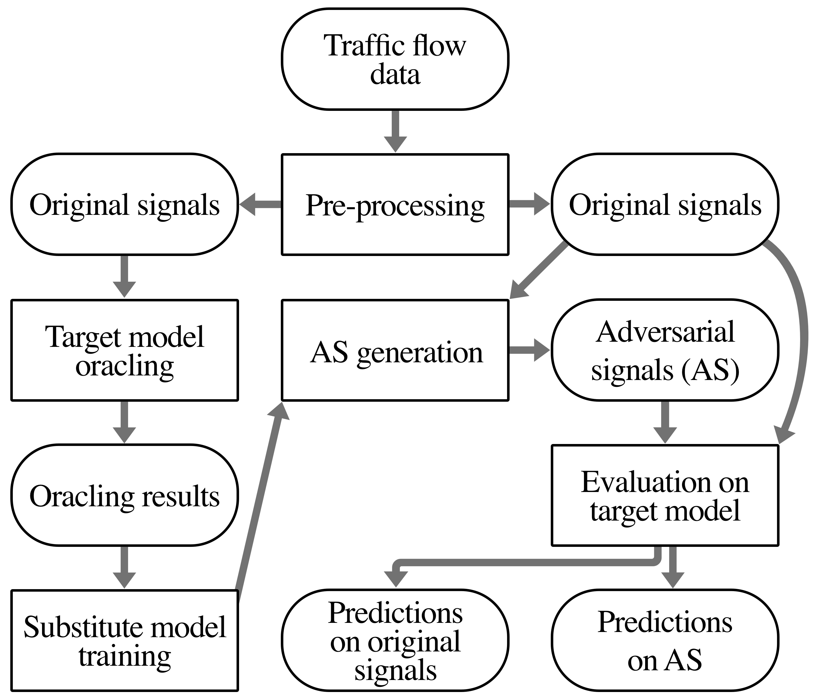
Figure 1: Systematic diagram of our framework. Network-wide traffic flow data is pre-processed and split into two parts, one is used by the adversary to oracle the target model to obtain input-output pairs for training the substitute model; the other is used by the adversary to generate adversarial signals based on the trained substitute model. The attack effectiveness is conducted on the target model using original signals and their corresponding adversarial signals.

The systematic diagram of our framework is shown in Fig. 1. The network-wide traffic flow data is pre-processed and split into input data for oracling the target model and ground-truth data for later evaluation of the attack effectiveness. The adversary feeds the input data into the target model and obtains corresponding output predictions. These input-output pairs are then used to train and tune a substitute model such that the substitute model produces similar prediction performance as the target model. Once this is done, adversarial signals are generated using the substitute model to attack the target model. In the following, we detail these steps.

TABLE I: LEFT: Average L2 distance between the 2 616 original signals and their adversarial signals as well as average L2 distance between the target model’s predictions on 2 616 original signals and their corresponding adversarial signals. All values are normalized by $10^{8}$. RIGHT: Performance evaluation of target models before and after the attack. Deep Learning models suffer severe degradation in terms of their prediction performance, compared to traditional models. DCRNN has the highest performance degradation among all models.

	Change on original signal (L2)		Change on prediction (L2)		Pre-attack RMSE	Post-attack RMSE		RMSE Degradation(%)
Model	FGSM	BIM	FGSM	BIM	N/A	FGSM	BIM	FGSM	BIM
GCGRNN	3.35	1.67	3.27	1.80	529.88	669.87	607.14	26.41%	14.58%
DCRNN	3.35	1.45	17.5	10.1	770.04	1186.41	1013.66	54.07%	31.63%
LR	3.35	1.45	3.16	1.38	1870.43	1916.83	1891.21	2.48%	1.11%
HA	132	129	0	0	935.46	935.46	935.46	0	0

IV-1 Data pre-processing

The traffic flow data is obtained from PeMS [26], which consists of hourly data from Jan 1, 2018 to Jun 30, 2019 of 150 sensors in Los Angeles, California. To prepare this network-wide data for multi-step prediction, 12 timesteps of data in the past are treated as inputs and next 12 timesteps of data are treated as outputs (i.e., ground truth). In total, we obtain 13 081 network-wide, 12-step traffic flow input-output data.

IV-2 Substitute model training

In order to train the substitute model, 9 157 (sampled from 13 081) input data is used to oracle the target model to obtain the corresponding predictions (which are different from the ground-truth output data for the 9 157 input data). These input-output pairs form our training data for the substitute model, which are z-score normalized using:

$$\operatorname*{\mathbf{x}}=(\operatorname*{\mathbf{x}}-{\mu})/{\sigma},$$ (5)

where ${\mu}$ and ${\sigma}$ are the mean and standard deviation of the 9 157 input data, respectively.

The substitute model is chosen to be the 50-layered residual network (ResNet-50) [34] as it achieves state of the art performance in time series classification on various UCR datasets [35]. To make the model more suitable for our purpose, we alter the model’s architecture by removing the pooling operation from initial layers to better preserve temporal correlations embedded in traffic data, and change the input and output layers to match the prediction task of 150 sensors across 12 timesteps. For each target model examined (four in total), a substitute model with randomly initialized parameters and the same set of hyperparameters is trained, using the 9 157 input-output pairs.

IV-3 Adversarial attack

In total, 2 616 adversarial signals are generated using both Fast Gradient Sign Method (FGSM) [23] and Basic Iterative Method (BIM) [24] by constraining the optimization program given in Eq. 2 with the maximum and minimum values of normalized inputs obtained from Eq. 5. This ensures that the adversarial signals are physically plausible, i.e., no negative traffic flows should occur. The adversarial signals generated on the substitute model are fed into the target model to obtain the “post-attack predictions” as the attack results. To measure the attack effectiveness, the inputs that are used to generate these adversarial signals are also fed into the target model to obtain “pre-attack predictions.” Root mean squared error (RMSE) is used as an evaluation metric to measure the model performance:

$$\textrm{RMSE}=\sqrt{\frac{1}{S\times F\times N}{\sum_{{i}}^{S}}{\sum_{{d}}^{F}}{\sum_{{n}}^{N}}{(y^{i}_{dn}-\hat{y}^{i}_{dn})}^{2}},$$ (6)

where $S$ = 2 616 is the number of adversarial signals; $F$ = 12 is the number of timesteps; $N$ = 150 is the number of sensors; $y_{dn}$ is the ground-truth data from PeMS and $\hat{y}_{dn}$ is either the “post-attack prediction” or “pre-attack predcition”. Denoting $\text{RMSE}_{pre}$ the difference between “pre-attack predictions” and the ground-truth, and $\text{RMSE}_{post}$ the difference between “post-attack predictions” and the ground-truth, the performance degradation is calculated as

$$\textrm{RMSE Degradation}=\frac{\textrm{RMSE}_{post}-\textrm{RMSE}_{pre}}{\textrm{RMSE}_{pre}}.$$ (7)

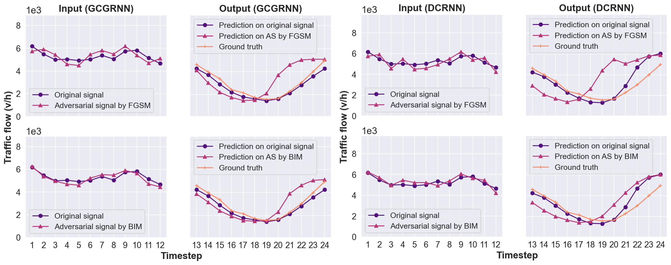
Figure 2: Examples of original signals and their corresponding adversarial signals’ impact on model prediction results. For both GCGRNN and DCRNN, we can see that the adversarial signals can cause large deviation between the prediction results and the ground truth than the original signals.

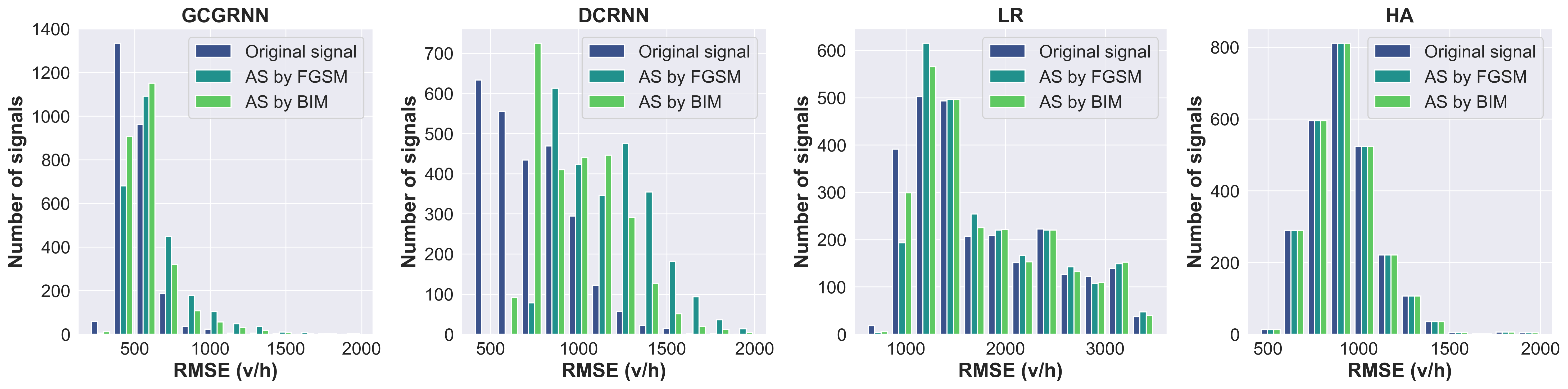
Figure 3: The RMSE distributions on both original signals and their adversarial signals (AS) of four target models ($2~{}616$ in total). Between GCGRNN and DCRNN, DCRNN shows larger distribution shift in RMSE values, which demonstrates the comparative robustness of GCGRNN against adversarial attacks. For LR, the shift is marginal; for HA, no shift is observed. These results demonstrate that traditional models can be more robust or even immune against adversarial attacks.

V Experiments

In this section, we first describe the experiment set-up and then present and discuss the experiment results. All experiments are conducted using an Intel(R) Core(TM) i7-10700 CPU, a Nvidia RTX 2080 SUPER GPU, and 32G RAM. PyTorch [36] is used to implement the substitute model and Advertorch [37] is used to generate adversarial signals.

The training data obtained by oracling the four pre-trained target models is respectively used to train four substitute models under the objective to minimize RMSE. The values of the hyperparameters are as follows: learning rate $=0.005$, optimizer $=$ Adam [38], batch size $=24$, number of epochs $=50$. To generate adversarial signals, RMSE is used as the cost function for both FGSM (with $\varepsilon=0.2$) and BIM (with $\alpha=0.05,~{}\varepsilon=0.2$, number of iterations $=10$). The upper and lower limit constraints on the optimization program in Eq. 2 are set to $3.49$ and $-1.89$, respectively.

Table I LEFT shows the results of using L2 distance as the metric to measure 1) the difference between the original signal and its corresponding adversarial signal and 2) the difference between the target model’s prediction on the original signal and the corresponding adversarial signal. Except for HA, the changes produced on the original signal by FGSM ($3.35\times 10^{8}$) are almost doubled than that of BIM ($1.67\times 10^{8}$, $1.45\times 10^{8}$), indicating that the adversarial signal from BIM are in general closer to the original signals than those from FGSM. For HA, the changes produced by FGSM ($1.32\times 10^{10}$) and BIM ($1.29\times 10^{10}$) to the original signals are much higher.

This may due to the inability of the substitute model to mimic HA’s behaviour: HA makes a periodic assumption on traffic state prediction i.e., to make a prediction on next 12 timesteps from an input of 12 historical timesteps, it does not use the input flow values, rather it looks at the hours of day, and day of the week (assuming period = week) of the input and averages the flow values over the same hours of day on the same day of the week from previous weeks. The substitute model makes predictions based on the learned features from the flow values of 12 historical timesteps, which does not contain periodic information. In other words, there is no way to tell if two network-wide multi-step inputs belong to the same period (e.g., the same hours of the same day of week). As a result, the substitute model fails to learn HA’s behavior, causing FGSM and BIM to produce large changes to the input signal while maximizing RMSE.

Regarding the changes on predictions, for GCGRNN and LR, changes under FGSM ($3.27\times 10^{8}$, $3.16\times 10^{8}$) are almost doubled than that of the changes under BIM ($1.80\times 10^{8}$, $1.38\times 10^{8}$). These changes are similar to the changes produced on the original signals to craft adversarial signals using FGSM and BIM respectively. In contrast, no changes are produced on the predictions for HA, this is again explained by the periodic assumption of HA since HA does not consider the flow values in the current input rather it considers the historical periods that it belongs. Hence, changes produced on current input cannot influence the prediction.

DCRNN suffers the largest changes at $17.5\times 10^{8}$ under FGSM and $10.1\times 10^{8}$ under BIM, indicating that the substitute model highly resembles DCRNN. Fig. 2 shows the predictions of GCGRNN and DCRNN on both original signals and their corresponding adversarial signals from either FGSM or BIM. As shown, the adversarial signals can cause much larger deviation between the model prediction and the ground truth than that of the original signals.

Table I RIGHT gives information about the target model predictions before the attack, after the attack, and RMSE degradation. Under no attack, GCGRNN has the smallest RMSE of $529.88$, which has increased to $699.87~{}(26.41\%~{}\text{RMSE degradation})$ using FGSM and $607.14~{}(14.58\%~{}\text{RMSE degradation})$ using BIM under adversarial attacks, respectively. The highest performance drop is for DCRNN where the RMSE of $770.4$ under no attack has increased to $1186.41~{}(54.07\%~{}\text{RMSE degradation})$ using FGSM and $1013.66~{}(31.63\%~{}\text{RMSE degradation})$ using BIM under adversarial attacks, respectively. The RMSE distributions on both original signals and their adversarial signals are shown in Fig. 3. DCRNN corresponds to more dramatic distribution shift to higher RMSE values than GCGRNN, which demonstrates the comparative robustness of GCGRNN against adversarial attacks than DCRNN.

For traditional models’ performance shown in Table I RIGHT, LR operates at high RMSE under no attack ($1870.43$) because of the linearity assumption (linearly combines historical timesteps for prediction). The RMSE has increased to $1916.83~{}(2.48\%~{}\text{RMSE degradation})$ using FGSM and $1891.21~{}(1.11\%~{}\text{RMSE degradation})$ using BIM under adversarial attacks, respectively. The “RMSE degradation” values for LR are relatively small compared to that for GCGRNN and DCRNN. From Table I LEFT, we can see that although the “change on prediction” under both FGSM and BIM for LR are similar to “change on prediction” for GCGRNN, the difference between “Pre-attack RMSE” and “Post-attack RMSE” is higher for GCGRNN than LR. This indicates that for LR, although the predictions on adversarial signals are far from predictions on original signals, their distances to the ground truth remain similar, i.e., the LR’s prediction already has high RMSE due to the model limitation in capturing temporal correlations embedded in historical traffic flow. In case of HA, the performance remains invariant to any attack, i.e., RMSE remains the same for original signals and adversarial signals due to the periodicity assumption explained before.

The lower prediction performance of both traditional models under no attack, due to their inability to accurately capture spatial and temporal correlations embedded in traffic data (owing to their simplistic assumptions of either linearity (LR) or periodicity (HA)), may be a contributor to their robustness. As can seen from Fig. 3, there exists marginal distribution shift to higher RMSE values for LR and no distribution shift for HA.

VI Conclusion and Future Work

In this work, we propose a black-box adversarial attack framework where an adversary can attack traffic state prediction models using publicly available dataset to oracle a target model, train a substitute model on prediction results, and attack the target model using the produced adversarial signals based on the substitute model. We have analyzed two deep learning models and two traditional models and find that traditional models are more robust to the proposed adversarial attack. Among the deep learning models, we find that GCGRNN is comparatively more robust against adversarial attacks than DCRNN.

There are many future research directions of this work. First of all, the input data for oracling the target model is complete and accurate. It would be interesting to study the influence of compressing data [39] or even missing data [40] on the attack. Secondly, our work could be extended to adversarial attacks on other traffic measurements such as speed and travel time. Another interesting topic is to study the impact of adversarial attack on existing techniques to navigate and coordinate autonomous vehicles [41, 42], which heavily rely on accurate prediction of traffic states to operate. This line of research can benefit from the use of virtual traffic platforms [43, 44] for experimenting, since the real-world deployment of the algorithms has safety implications.

Last but not least, deep learning models (e.g., GCGRNN and DCRNN) are data-driven, which in general do not consider domain knowledge such as short-term seasonality (e.g., weekdays vs. weekend), long-term seasonality (e.g., Spring vs. Summer), and special events (e.g., holidays). Given that the real-world traffic is associated with such information, it would be worthwhile to explore their inclusion as a part of the input.

References

- [1] L. Lin, W. Li, and L. Zhu, “Network-wide multi-step traffic volume prediction using graph convolutional gated recurrent neural network,” Technical Report, 2021.
- [2] Y. Li, R. Yu, C. Shahabi, and Y. Liu, “Diffusion convolutional recurrent neural network: Data-driven traffic forecasting,” in International Conference on Learning Representations (ICLR), 2018.
- [3] M. S. Ahmed and A. R. Cook, Analysis of freeway traffic time-series data by using Box-Jenkins techniques, 1979, no. 722.
- [4] O. Anacleto, C. Queen, and C. J. Albers, “Multivariate forecasting of road traffic flows in the presence of heteroscedasticity and measurement errors,” Journal of the Royal Statistical Society: Series C (Applied Statistics), vol. 62, no. 2, pp. 251–270, 2013.
- [5] L. Zhang, Q. Liu, W. Yang, N. Wei, and D. Dong, “An improved k-nearest neighbor model for short-term traffic flow prediction,” Procedia-Social and Behavioral Sciences, vol. 96, pp. 653–662, 2013.
- [6] Y. Lv, Y. Duan, W. Kang, Z. Li, and F.-Y. Wang, “Traffic flow prediction with big data: a deep learning approach,” IEEE Transactions on Intelligent Transportation Systems, vol. 16, no. 2, pp. 865–873, 2014.
- [7] L. Lin, W. Li, and S. Peeta, “Predicting station-level bike-sharing demands using graph convolutional neural network,” in Transportation Research Board 98th Annual Meeting (TRB), 2019.
- [8] L. Lin, W. Li, H. Bi, and L. Qin, “Vehicle trajectory prediction using LSTMs with spatial-temporal attention mechanisms,” IEEE Intelligent Transportation Systems Magazine, 2021.
- [9] S. R. Chandra and H. Al-Deek, “Predictions of freeway traffic speeds and volumes using vector autoregressive models,” Journal of Intelligent Transportation Systems, vol. 13, no. 2, pp. 53–72, 2009.
- [10] X. Ma, Z. Tao, Y. Wang, H. Yu, and Y. Wang, “Long short-term memory neural network for traffic speed prediction using remote microwave sensor data,” Transportation Research Part C: Emerging Technologies, vol. 54, pp. 187–197, 2015.
- [11] L. Lin, J. C. Handley, Y. Gu, L. Zhu, X. Wen, and A. W. Sadek, “Quantifying uncertainty in short-term traffic prediction and its application to optimal staffing plan development,” Transportation Research Part C: Emerging Technologies, vol. 92, pp. 323–348, 2018.
- [12] P. Cai, Y. Wang, G. Lu, P. Chen, C. Ding, and J. Sun, “A spatiotemporal correlative k-nearest neighbor model for short-term traffic multistep forecasting,” Transportation Research Part C: Emerging Technologies, vol. 62, pp. 21–34, 2016.
- [13] W. Li, D. Nie, D. Wilkie, and M. C. Lin, “Citywide estimation of traffic dynamics via sparse GPS traces,” IEEE Intelligent Transportation Systems Magazine, vol. 9, no. 3, pp. 100–113, 2017.
- [14] W. Li, M. Jiang, Y. Chen, and M. C. Lin, “Estimating urban traffic states using iterative refinement and wardrop equilibria,” IET Intelligent Transport Systems, vol. 12, no. 8, pp. 875–883, 2018.
- [15] Y. Luo, Q. Liu, H. Zhu, H. Fan, T. Song, C. W. Yu, and B. Du, “Multistep flow prediction on car-sharing systems: A multi-graph convolutional neural network with attention mechanism,” 2019.
- [16] A. K. Haghighat, V. Ravichandra-Mouli, P. Chakraborty, Y. Esfandiari, S. Arabi, and A. Sharma, “Applications of deep learning in intelligent transportation systems,” Journal of Big Data Analytics in Transportation, vol. 2, no. 2, pp. 115–145, 2020.
- [17] S. Wang, K. Wei, L. Lin, and W. Li, “Spatial-temporal analysis of COVID-19’s impact on human mobility: the case of the united states,” in The 20th and 21st Joint COTA International Conference of Transportation Professionals, 2021.
- [18] L. Lin, F. Shi, and W. Li, “Assessing inequality, irregularity, and severity regarding road traffic safety during covid-19,” Scientific Reports, vol. 11, p. 13147, 2021.
- [19] C. Szegedy, W. Zaremba, I. Sutskever, J. Bruna, D. Erhan, I. Goodfellow, and R. Fergus, “Intriguing properties of neural networks,” arXiv preprint arXiv:1312.6199, 2013.
- [20] K. Eykholt, I. Evtimov, E. Fernandes, B. Li, A. Rahmati, C. Xiao, A. Prakash, T. Kohno, and D. Song, “Robust physical-world attacks on deep learning visual classification,” in Proceedings of the IEEE Conference on Computer Vision and Pattern Recognition, 2018, pp. 1625–1634.
- [21] C. Song and V. Shmatikov, “Fooling ocr systems with adversarial text images,” arXiv preprint arXiv:1802.05385, 2018.
- [22] S. Dadras, R. M. Gerdes, and R. Sharma, “Vehicular platooning in an adversarial environment,” in Proceedings of the 10th ACM Symposium on Information, Computer and Communications Security, 2015, pp. 167–178.
- [23] I. J. Goodfellow, J. Shlens, and C. Szegedy, “Explaining and harnessing adversarial examples,” arXiv preprint arXiv:1412.6572, 2014.
- [24] A. Kurakin, I. Goodfellow, and S. Bengio, “Adversarial machine learning at scale,” arXiv preprint arXiv:1611.01236, 2016.
- [25] N. Papernot, P. McDaniel, and I. Goodfellow, “Transferability in machine learning: from phenomena to black-box attacks using adversarial samples,” arXiv preprint arXiv:1605.07277, 2016.
- [26] “Caltrans performance measurement system (pems),” http://pems.dot.ca.gov, accessed: 2021-02-28.
- [27] L. Zhao, Y. Song, C. Zhang, Y. Liu, P. Wang, T. Lin, M. Deng, and H. Li, “T-gcn: A temporal graph convolutional network for traffic prediction,” IEEE Transactions on Intelligent Transportation Systems, vol. 21, no. 9, pp. 3848–3858, 2019.
- [28] X. Ma, Z. Dai, Z. He, J. Ma, Y. Wang, and Y. Wang, “Learning traffic as images: a deep convolutional neural network for large-scale transportation network speed prediction,” Sensors, vol. 17, no. 4, p. 818, 2017.
- [29] Z. Cui, K. Henrickson, R. Ke, and Y. Wang, “Traffic graph convolutional recurrent neural network: A deep learning framework for network-scale traffic learning and forecasting,” IEEE Transactions on Intelligent Transportation Systems, 2019.
- [30] Y. Wang, D. W. M. Chia, and Y. Ha, “Vulnerability of deep learning model based anomaly detection in vehicle network,” in 2020 IEEE 63rd International Midwest Symposium on Circuits and Systems (MWSCAS). IEEE, 2020, pp. 293–296.
- [31] R. A. Rixey, “Station-level forecasting of bikesharing ridership: Station network effects in three us systems,” Transportation research record, vol. 2387, no. 1, pp. 46–55, 2013.
- [32] Y. Kamarianakis, W. Shen, and L. Wynter, “Real-time road traffic forecasting using regime-switching space-time models and adaptive lasso,” Applied stochastic models in business and industry, vol. 28, no. 4, pp. 297–315, 2012.
- [33] B. L. Smith and M. J. Demetsky, “Traffic flow forecasting: comparison of modeling approaches,” Journal of transportation engineering, vol. 123, no. 4, pp. 261–266, 1997.
- [34] K. He, X. Zhang, S. Ren, and J. Sun, “Deep residual learning for image recognition,” in Proceedings of the IEEE conference on computer vision and pattern recognition, 2016, pp. 770–778.
- [35] Z. Wang, W. Yan, and T. Oates, “Time series classification from scratch with deep neural networks: A strong baseline,” in 2017 International joint conference on neural networks (IJCNN). IEEE, 2017, pp. 1578–1585.
- [36] A. Paszke, S. Gross, S. Chintala, G. Chanan, E. Yang, Z. DeVito, Z. Lin, A. Desmaison, L. Antiga, and A. Lerer, “Automatic differentiation in pytorch,” 2017.
- [37] G. W. Ding, L. Wang, and X. Jin, “Advertorch v0. 1: An adversarial robustness toolbox based on pytorch,” arXiv preprint arXiv:1902.07623, 2019.
- [38] D. P. Kingma and J. Ba, “Adam: A method for stochastic optimization,” in International Conference on Learning Representations, 2015.
- [39] L. Lin, W. Li, and S. Peeta, “Efficient data collection and accurate travel time estimation in a connected vehicle environment via real-time compressive sensing,” Journal of Big Data Analytics in Transportation, vol. 1, no. 2, pp. 95–107, 2019.
- [40] W. Li, D. Wolinski, and M. C. Lin, “City-scale traffic animation using statistical learning and metamodel-based optimization,” ACM Trans. Graph., vol. 36, no. 6, pp. 200:1–200:12, Nov. 2017.
- [41] C. Wu, A. M. Bayen, and A. Mehta, “Stabilizing traffic with autonomous vehicles,” in 2018 IEEE International Conference on Robotics and Automation (ICRA). IEEE, 2018, pp. 6012–6018.
- [42] W. Li, D. Wolinski, and M. C. Lin, “ADAPS: Autonomous driving via principled simulations,” in IEEE International Conference on Robotics and Automation (ICRA), 2019, pp. 7625–7631.
- [43] D. Wilkie, J. Sewall, W. Li, and M. C. Lin, “Virtualized traffic at metropolitan scales,” Frontiers in Robotics and AI, vol. 2, p. 11, 2015.
- [44] Q. Chao, H. Bi, W. Li, T. Mao, Z. Wang, M. C. Lin, and Z. Deng, “A survey on visual traffic simulation: Models, evaluations, and applications in autonomous driving,” Computer Graphics Forum, vol. 39, no. 1, pp. 287–308, 2020.