GP-MOOD: A positive-preserving high-order finite volume method for hyperbolic conservation laws

Abstract

We present an a posteriori shock-capturing finite volume method algorithm called GP-MOOD that solves a compressible hyperbolic conservative system at high-order solution accuracy (e.g., third-, fifth-, and seventh-order) in multiple spatial dimensions. The GP-MOOD method combines two methodologies, the polynomial-free spatial reconstruction methods of GP (Gaussian Process) and the a posteriori detection algorithms of MOOD (Multidimensional Optimal Order Detection). The spatial approximation of our GP-MOOD method uses GP’s unlimited spatial reconstruction that builds upon our previous studies on GP reported in Reyes et al., Journal of Scientific Computing, 76 (2017) and Journal of Computational Physics, 381 (2019). This paper focuses on extending GP’s flexible variability of spatial accuracy to an a posteriori detection formalism based on the MOOD approach. We show that GP’s polynomial-free reconstruction provides a seamless pathway to the MOOD’s order cascading formalism by utilizing GP’s novel property of variable $(2R+1)$th-order spatial accuracy on a multidimensional GP stencil defined by the GP radius $R$, whose size is smaller than that of the standard polynomial MOOD methods. The resulting GP-MOOD method is a positivity-preserving method. We examine the numerical stability and accuracy of GP-MOOD on smooth and discontinuous flows in multiple spatial dimensions without resorting to any conventional, computationally expensive a priori nonlinear limiting mechanism to maintain numerical stability.

1 Introduction

Nonlinear shock waves and discontinuities are ubiquitous in compressible flows. Therefore, a strong gradient control algorithm is an essential building block in a numerical method for compressible flow simulations. A well-suited numerical discretization should be accompanied by a robust mechanism that can feel such gradient flows and evolve its solution stably and accurately, suppressing any adverse evolution of numerical oscillations and unphysical states. Practitioners have devised novel ways to meet such computational needs to maximize solution accuracy (at the cost of lowering numerical dissipation) on smooth flows while maximizing numerical stability (or increasing numerical dissipation at the cost of lowering solution accuracy) on strong gradient flows. Numerically, the corresponding resolution can be classified as one of the two approaches, namely: an a priori method and an a posteriori method, depending on how a given method detects and controls smooth vs. non-smooth local flows.

A more popular and traditional path has been the a priori approach, in which all cells are spatially discretized by utilizing one or more nonlinear limiting procedures, integrated with a stable temporal update to the next time step. Well-known examples of a priori limiting methods include second-order piecewise linear TVD (Total Variation Diminishing) methods (e.g.,  [1, 2, 3, 4]), higher-order polynomial approximations such as piecewise parabolic method (PPM) [5, 6], essentially non-oscillatory methods (ENO) (e.g.,  [7, 8]), weighted ENO (WENO) methods (e.g.,  [9, 10, 11, 12]) and other variants such as central WENO (CWENO) [13, 14, 15, 16], Hermite WENO (HWENO) [17], adaptive-order WENO (AO-WENO) [18, 19], polynomial-free Gaussian Process WENO (GP-WENO) [20, 21, 22], to name a few.

In these shock-capturing methods, nonlinear mechanisms or switches are necessary to detect the magnitude of local flow gradients in an a priori fashion to evolve numerical solutions stably while meeting underlying physical principles (e.g., positivity, conservation). From the computational perspective, major drawbacks in these a priori nonlinear switches are two-fold: “the computational expense” due to the required cell-by-cell calculation of nonlinear limiters and “the presence of unavoidable numerical dissipation” resulting in degraded solution accuracy. In [23], Kent et al. studied the impact of monotone and quasi-monotone limiters on effective grid resolutions for finite difference (FD) and finite volume (FV) methods. The study shows that a large increase in numerical diffusion and dispersion errors is observed at the first time step, significantly reducing the effective grid resolution compared to the corresponding unlimited schemes. The disparity between the limited and unlimited schemes then grows at a slower rate as simulations progress to longer time steps.

Compared to the a priori approach, the a posteriori approach is a relatively newer paradigm for compressible shock-capturing schemes. For this approach, there have been growing interests in the so-called Multidimensional Optimal Order Detection (MOOD) method in the past decade, which takes a different strategy in handling shocks and discontinuities in compressible flow simulations. Since its first introduction in [24], the MOOD method has become a new a posteriori detection principle alternative to the conventional a priori shock-capturing techniques based on nonlinear limiting procedures. The original MOOD in [24] focused on developing high-order (up to third-order) two-dimensional polynomial approximations on unstructured grids. This study introduced the first idea of its kind where the initial unlimited polynomial order of accuracy cascades down to lower ones until a discrete candidate solution on each cell meets a predefined admissibility condition called the Discrete Maximum Principle (DMP). In this context, the troubled cells that fail to meet the prescribed DMP condition need to be recomputed locally, hence referred to as an a posteriori scheme. In [25], the accuracy of the MOOD method was extended to sixth-order on unstructured grids with an improved detection criterion called the $u$2 detection that relaxes the order-reduction criterion on smooth extrema. Besides, the positivity-preserving property under an admissible CFL (Courant-Fredirichs-Lewy) condition was made explicit by imposing the Physical Admissibility Detection (PAD) that checks the positivity of density and pressure variables on each cell. The MOOD method was further extended to general three-dimensional unstructured meshes with simplifications of the $u$2 detection [26, 27]; to a third-order FV adaptive mesh refinement (AMR) scheme in [28].

The MOOD paradigm of “repeat-until-valid” has also been adopted in the Discontinuous Galerkin (DG) method, where the first pass of discrete updates is done by a target high-order unlimited DG solver. Then, the invalid cells that fail to meet prescribed admissibility conditions such as PAD and Numerical Admissibility Detection (NAD) are recomputed using other more stable (but lower accurate) limited solvers (such as WENO) at a more refined subcell resolution on each of those invalid cell, e.g., see examples of the MOOD limiter in ADER-DG applications  [32, 33].

On the other hand, there has been a new attempt [34] to use a trained Neural Network (NN) with hidden layers and few perceptrons to design an NN-based classification model. In this NN approach, the standard a posterior MOOD detection strategy is replaced by an educated guess of the appropriate order of polynomial accuracy. Thus, the potential imbalance in parallel efficiency caused by the extra recomputing need in the standard MOOD treatment could be ameliorated. Moreover, the NN-based approach alters the original a posteriori nature of the MOOD paradigm to a trained a priori version, which would be better suited for extending the MOOD method to an implicit scheme. Although promising, the work in [34] has some limitations; namely, it only explored shallow NNs of two hidden layers; investigated 1D tests only; trained their NNs on a relatively moderate size of a training set; the positivity and NAN checks are not in the part of NNs but imposed separately as part of the a posteriori MOOD loop.

There are two core building blocks in the MOOD method. The first building block is the MOOD detection criteria themselves to tag invalid cells. These problematic cells are subsequently recomputed using a more stable but less accurate discretization method, repeating the so-called MOOD iterative loop until they become valid. The second building block is a set of multiple choices (at least two, e.g., a high-order unlimited method and a first-order method) of spatial discretization methods so that the invalid cells become valid physically (i.e., PAD) and numerically (i.e., NAD) at the end of the MOOD loop. To date, the MOOD method has exclusively employed the use of multidimensional polynomial reconstruction [24, 25, 26, 27, 34]. By far, piecewise polynomial reconstruction and interpolation of stencil data have been among the most understood and well-established mathematical tools in computing discrete approximations to underlying functions in computational fluid dynamics (CFD).

Regardless, there seem at least two challenges in function approximations using piecewise multidimensional polynomials. The first issue appears to be well-known complications where the interpolated/reconstructed solutions of piecewise multidimensional polynomials may lead to an ill-conditioned or unsolvable linear system. One workaround could be to utilize a tensor product of one-dimensional $n$th-order (or $(n-1)$th degree) polynomials  [35, 36, 37] whose degrees of freedom (i.e., the number of unknown polynomial coefficients) is $\mbox{DoF}(n)=n(n+1)/2$. Another workaround is to solve a least-squares problem (LSP) to compute polynomial coefficients with a number of stencil points larger than $\mbox{DoF}(n)$ [38, 39]. The LSP pathway is also taken by the existing MOOD methods  [24, 25, 26, 27, 28, 34], wherein 2D at least 5 cells are required for 2nd-order MOOD, 8 cells for 3rd-order MOOD, 16 cells for 4th-order MOOD, 20 cells for 5th-order MOOD, and 26 cells for 6th-order MOOD [25]. The second challenging issue is the computational cost. Ideally, in the existing MOOD approach, a new least-squares solution is required for all cells in the first pass and for each troubled cell at every subsequent MOOD iteration to compute lower-order polynomials. To minimize this computationally intensive polynomial reconstruction, an effort of ‘truncating’ the highest degree polynomial to lower-order polynomials was proposed in [24], although it was found later to be undesirable at discontinuities for 3rd-order or higher MOOD methods [25].

Here lies the main emphasis of this paper. In the context of FV MOOD, we propose a new set of Gaussian Process (GP) reconstruction methods that are polynomial-free and computationally efficient. We will show that the prime advantage in our GP reconstruction is afforded by GP’s re-usable high-order spatial reconstructors that seamlessly vary its solution accuracy. Thereby, we advance the MOOD’s second building block significantly in solution accuracy, stability, and efficiency. Our approach builds around the recent developments of GP methods  [20, 21, 22]. First introduced by Reyes et al. [20], FV GP reconstruction has shown a versatile selectable-order property in modeling the 1D Euler equations [20]. The FV GP method followed WENO’s a priori shock-handling control with modified GP smoothness indicators, called GP-WENO. An extension of GP-WENO to a full 3D FD method (FD-prim) was reported in [21]. In the most recent work [22] by Reeves et al., the GP-WENO method was extended to a 3rd-order prolongation algorithm in FV AMR simulations using AMReX [40]. In addition, we further relax the existing MOOD admissibility conditions in the current study. This new relaxed detection strategy is found to be crucial for simulating key flow structures on some of the well-known benchmark test problems (e.g., non-systematic solution behaviors in the 1D Shu-Osher test in Section 5.2.1; the diagonal jet formation in the 2D implosion test in Section 5.2.4). The new relaxation improves the issue in the existing MOOD method, in which the order decrement takes place on cells where the local flow is weakly compressible but has not yet built steep gradients. Such local flows are an important powerhouse to trigger a more nonlinear regime (e.g., formations of shocks, vortex roll-ups, reflected jets) in the subsequent flow dynamics. However, in the existing MOOD method, we observed that a low order method is activated too soon on such cells, which often suppresses the onset of such signature flow structures by the excessive numerical dissipation.

We organize the paper as follows. In Section 2 we briefly review the discretization strategy of the existing MOOD method. We present a group of unlimited, selectable-order GP reconstruction methods whose spatial accuracy is linearly varying at $(2R+1)$th-order with an integer GP radius $R$. Demonstrated in this paper include GP methods of 3rd-order ($R=1$), 5th-order ($R=2$), and 7th-order ($R=3$). In Section 2 we describe a new relaxed MOOD strategy that combines a multidimensional shock-detector and the MOOD method. A description of a step-wise implementation of GP-MOOD is given in Section 4. The test results of our new GP-MOOD method are presented in Section 5. We conclude our paper with a brief summary in Section 6.

2 Finite volume discretization of GP-MOOD

The FV spatial discretization of the GP-MOOD method is introduced in this section. We focus on designing a set of selectable-order GP-MOOD algorithms on Cartesian grid configurations, which reconstruct point-wise Riemann states at cell faces using cell-centered volume averages. As will be shown, the GP reconstructor is a covariance kernel-based posterior mean function that computes the $(2R+1)$th-order accurate Riemann states at cell faces directly (i.e., without the conventional Taylor series expansion) from the cell-centered average values on the multidimensional GP stencil of radius $R$. The Riemann states are computed at multiple Gaussian quadrature points on each cell face to deliver the anticipated $(2R+1)$th spatial accuracy. The spatial solutions are temporally evolved with strong stability preserving Runge-Kutta (SSP-RK) methods.

2.1 Governing equations and the basic finite volume discretization form

We are interested in solving a general hyperbolic system of conservative laws in 2D,

$$\partial_{t}\mathbf{U}+\partial_{x}\mathbf{F}(\mathbf{U})+\partial_{y}\mathbf{G}(\mathbf{U})=0,$$ (1)

where $\mathbf{U}$ is the vector of conservative variables and $\bm{\mathcal{F}}=(\mathbf{F},\mathbf{G})$ are the flux functions in $x$- and $y$-direction. In the Euler equations in 2D, the conservative variables and the flux functions are defined as,

$$\mathbf{U}=\begin{bmatrix}\rho\\ \rho u\\ \rho v\\ \rho E\end{bmatrix},\quad\mathbf{F}(\mathbf{U})=\begin{bmatrix}\rho u\\ \rho u^{2}+p\\ \rho uv\\ u\left(\rho E+p\right)\end{bmatrix},\quad\mathbf{G}(\mathbf{U})=\begin{bmatrix}\rho v\\ \rho uv\\ \rho v^{2}+p\\ v\left(\rho E+p\right)\end{bmatrix},\quad$$ (2)

where $\rho$ denotes the fluid density, $u$ and $v$ represent the $x$ and $y$ fluid velocity respectively, and $\rho E$ is the total energy. The system is closed with an ideal gas equation of state (EoS), $p=(\gamma-1)\left(\rho E-\frac{1}{2}\rho({u^{2}+v^{2})}\right),$ where $\gamma$ is the ratio of specific heats. The hyperbolic system in Eq. (2) is physically admissible if both $p>0$ and $\rho>0$, and the numerical method that maintains the positivity property is referred to as a positivity-preserving method.

The basic form of the finite volume discretization of Eq. 1 is derived by integrating the equation over each cell $I_{ij}=[x_{i-1/2},x_{i+1/2}]\times[y_{j-1/2},y_{j+1/2}]$ and over a time interval $[t^{n},t^{n+1}]$, yielding

$$\overline{\mathbf{U}}^{n+1}_{ij}=\overline{\mathbf{U}}^{n}_{ij}-\Delta t\,\mathbb{F}_{\nabla},$$ (3)

where $\overline{\mathbf{U}}^{n}_{ij}$ is a vector of the volume-averaged conservative variables and $\mathbb{F}_{\nabla}$ is a collection of the rest of spatial derivatives terms, including the face-averaged and temporally-averaged flux in each spatial direction. A popular choice for the discrete temporal update in Eq. 3 for high-order simulations is to use either a one-step ADER method [29, 30, 31] or a multi-stage SSP-RK method [41, 42] (the latter is our choice in this paper).

It leaves us to determine how to update the spatial approximations of the relevant terms in $\mathbb{F}_{\nabla}$ to meet the expected high-order accuracy. To this end, we design a family of multidimensional FV reconstruction algorithms of GP with the following set of attentions [43, 25]:

• make a clear distinction between the integral quantities (e.g., face-averaged, volume-averaged) and the pointwise values,

• use volume-averaged conservative quantities in high-order reconstruction, viz., avoid the use of primitive variables in reconstruction, which often are derived by inappropriate nonlinear operations such as the $x$-velocity computed as a division of the volume-averaged $x$-momentum by the volume-averaged density, e.g., $u\leftarrow\overline{\rho u}/\overline{\rho}$ or $\overline{u}\leftarrow\overline{\rho u}/\overline{\rho}$,

• avoid any nonlinear operations that use inappropriately converted primitive variables to construct conservative variables and use them in the evolution of conservative solution updates, e.g., any nonlinear operations that use the $x$-velocity in (ii) to replace any volume-averaged conservative variables, $\overline{\rho u}\leftarrow(\overline{\rho})(\overline{u}$).

In this paper, we use a $q$-point Gaussian quadrature rule to approximate the face-averaged fluxes at $2q$-th order accuracy using $q$ many pointwise fluxes on each cell face. For the sake of simplicity, we assume a uniform Cartesian grid configuration in 2D. This gives us to write $\mathbb{F}_{\nabla}$ as

$$\mathbb{F}_{\nabla}=\frac{1}{\Delta x}\sum_{j_{g}=1}^{q}\omega_{j_{g}}\Big{(}\mathbf{F}^{*}_{i+1/2,j_{g}}-\mathbf{F}^{*}_{i-1/2,j_{g}}\Big{)}+\frac{1}{\Delta y}\sum_{i_{g}=1}^{q}\omega_{i_{g}}\Big{(}\mathbf{G}^{*}_{i_{g},j+1/2}-\mathbf{G}^{*}_{i_{g},j-1/2}\Big{)},$$ (4)

where $i_{g}$ and $j_{g}$ are the indices of the $q$-point Gaussian quadrature point locations on each $x$ and $y$ cell face; the corresponding $\omega_{i_{g}}$ and $\omega_{j_{g}}$ are the quadrature weights for the $2q$-th order numerical integration. The numerical fluxes $\mathbf{F}^{*}$ and $\mathbf{G}^{*}$ are pointwise fluxes at each respective cell face, obtained by solving the corresponding Riemann problems at the Gaussian quadrature points. A pair of high-order accurate pointwise Riemann states, $(\mathbf{U}_{L},\mathbf{U}_{R})$, are used as inputs to calculate the corresponding Riemann problems at each quadrature point. In each pair, the left $\mathbf{U}_{L}$ and the right $\mathbf{U}_{R}$ states are computed using a $(2R+1)$th-order GP reconstruction method that takes inputs of the volume-averaged cell-centered conservative variables $\overline{\mathbf{U}}^{n}_{ij}$ on a multidimensional GP stencil determined by the size of a GP radius $R$.

In the next section, we describe a family of $(2R+1)$th-order GP reconstruction methods. More specifically, we aim to provide a family of three GP solvers, including a 3rd-order GP method with $R=1$ (GP-R1), a 5th-order GP method with $R=2$ (GP-R2), and a 7th-order GP method with $R=3$ (GP-R3). It should be noted that our GP algorithm is general and is not limited to the 7th-order GP-R3 method. As expected, however, the computational cost increases as $R$ increases, primarily due to the increase in the size of the resulting linear system to solve and the increase in the number of the needed Gaussian quadrature points. For this reason, we present our GP method up to 7th-order in this paper.

2.2 The GP stencil

This section presents how to configure local GP stencils in the context of a two-dimensional FV reconstruction. The $(2R+1)$th-order GP reconstruction operates on:

• Input: a vector $\mathbf{q}$ consisting of the volume-averaged conservative variables (e.g., $\overline{\rho}^{n}_{ij}$) on a 2D local GP stencil of radius $R$, where the GP radius $R$ is a runtime parameter.

• Output: an unlimited $(2R+1)$th-order accurate conservative pointwise Riemann state of the same input variable (e.g., density) at each Gaussian quadrature point (e.g., $\rho_{*}=\rho(\mathbf{x}_{*})$, where $\mathbf{x}_{*}=(x_{i\pm 1/2},y_{j_{g}})$ or $\mathbf{x}_{*}=(x_{i_{g}},y_{j\pm 1/2})$)

Let us first give a geometrical description of how our GP local stencil of size $R$ is configured. We begin with the simplest case with $R=1$ for the 3rd-order GP reconstruction. The GP radius $R$ is an integer value in the unit of grid spacing, $\Delta x$ and $\Delta y$. For example, in a 2D uniform grid configuration the GP stencil of $R=1$ defines a five-point cross-shape stencil that extends the local stencil centered at $\mathbf{x}_{ij}=(x_{i},y_{j})$ to one neighboring cell in each $x$ and $y$ direction, drawing hypothetically a blocky-diamond in 2D around $\mathbf{x}_{ij}$. In general, $\Delta x$ could be different from $\Delta y$, in which case the GP stencil becomes a stretched-cross consisting of the five volume-averaged data around $\mathbf{x}_{ij}$.

Fig. 1 illustrates how the GP-R1 stencil is configured around the central cell $\mathbf{x}_{ij}$. For exposition purposes, we also show ordered labeling, which is used for reshaping the five volume-averaged quantities at those cells in Fig. 1 into a one-dimensional array, denoted by $\overline{\mathbf{q}}_{ij}$. At each timestep $t=t^{n}$, the five local volume-averaged conservative variables, $\bar{q}_{m}=\bar{q}(\mathbf{x}_{m},t^{n})$, $m=1,\dots,5$, are cast into $\overline{\mathbf{q}}_{ij}$ in the order as shown in Fig. 1, starting from the data $\bar{q}_{1}$ at the central cell $\mathbf{x}_{ij}$,

$$\overline{\mathbf{q}}_{ij}=\left(\bar{q}_{1},\bar{q}_{2},\bar{q}_{3},\bar{q}_{4},\bar{q}_{5}\right)^{T}.$$ (5)

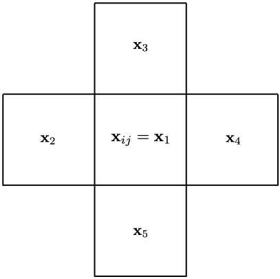
Figure 1: The five-point GP stencil of radius $R=1$ for the 3rd-order GP reconstruction method. The ordered labeling illustrates how the local volume-averaged conservative variables at $t=t^{n}$ are rearranged into a one-dimensional five-point array, $\overline{\mathbf{q}}_{ij}$.

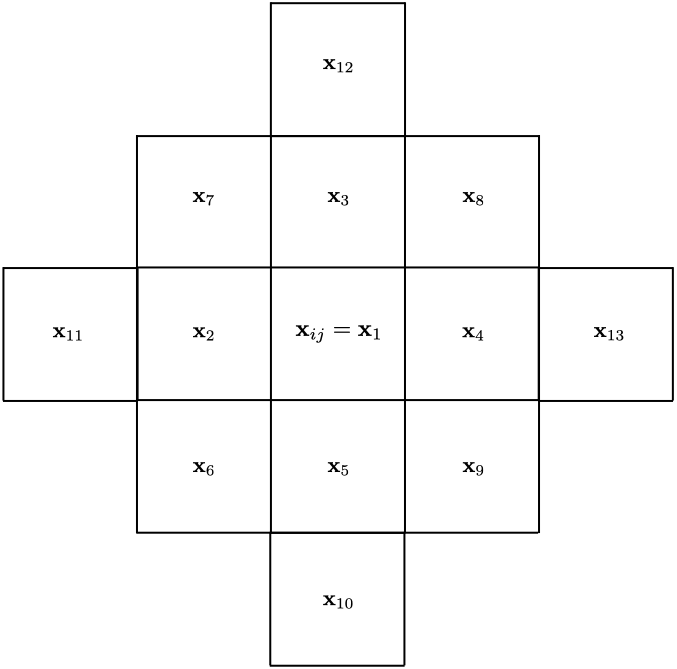
(a)

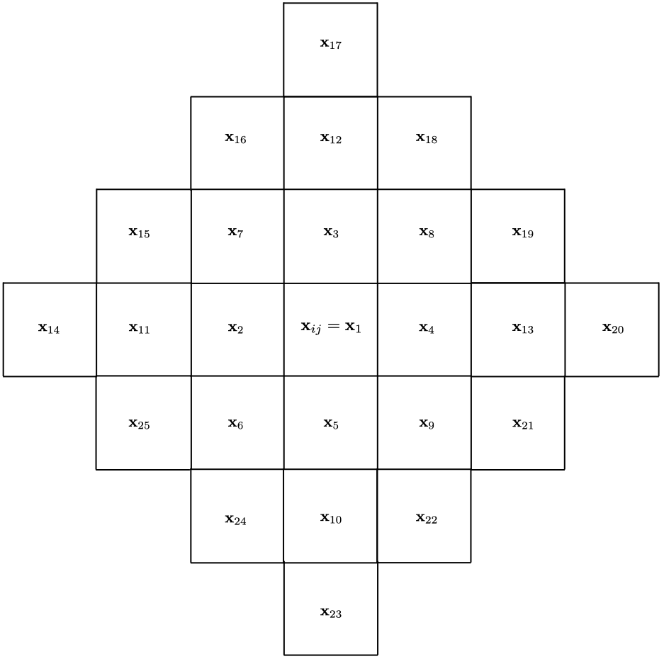
(b)

Figure 2: (a) The 13-point GP stencil of radius $R=2$ for the 5th-order GP reconstruction method. (b) The 25-point GP stencil of radius $R=3$ for the 7th-order GP reconstruction method. In both, the ordered labeling illustrates how the local volume-averaged conservative variables at $t=t^{n}$ are rearranged into a one-dimensional five-point array, $\overline{\mathbf{q}}_{ij}$.

In a similar fashion, we form the blocky-diamond GP stencils that group the neighboring 13 cell data for the GP-R2 stencil in Fig. 2(a) and the 25 cell data for the GP-R3 stencil in Fig. 2(b). The one-dimensional array $\overline{\mathbf{q}}_{ij}$ will hold 13 cell data for GP-R2 and 25 for GP-R3, following the orderly fashion indicated in Fig. 2. This finalizes our discussion on the GP stencils for the 3rd-, 5th-, and 7th-order methods. We remark that the size of our GP stencils is smaller than the local stencil size of the existing polynomial-based MOOD methods at the same or comparable accuracy in 2D [25], e.g., 5 cells for the 2nd-order polynomial MOOD methods, 8 for 3rd-order, 20 for 5th-order, and 26 for 6th-order.

The orderly-grouped GP stencil data in $\overline{\mathbf{q}}_{ij}$ are used as inputs to the GP reconstructor. We extend our earlier work in [20] to designing two-dimensional GP reconstruction schemes that convert the local volume-averaged data $\overline{\mathbf{q}}_{ij}$ to a $(2R+1)$th-order accurate pointwise conservative quantity at each Gaussian quadrature point, $g_{m}$, as displayed in Fig. 3.

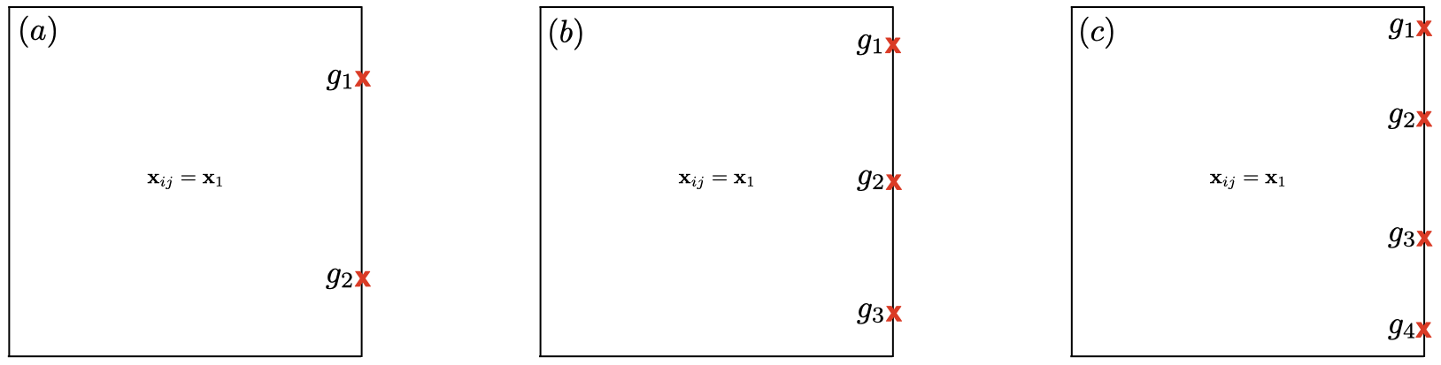
Figure 3: Multi-point Gaussian quadrature points, $g_{m}$, at the $x$-normal cell-face of the central cell $\mathbf{x}_{ij}=\mathbf{x}_{1}$. (a) The 4th-order two-point quadrature rule with two quadrature points is used with the 3rd-order GP-R1 method. (b) The 6th-order three-point quadrature rule with three quadrature points is used with the 5th-order GP-R2 method. (c) The 8th-order four-point quadrature rule with four quadrature points is used with the 7th-order GP-R3 method. The values of the quadrature points $g_{m}$ and the corresponding weights $\omega_{m}$ are given in Table 1.

Table 1: Multi-point Gaussian quadrature rules (QR) are used in combination with GP. The quadrature points, $g_{m}$, are tabulated over the reference interval $[-0.5,0.5]$ that maps to the unit length of each cell-face, e.g., $[y_{j-1/2},y_{j+1/2}]$ at the $x$-normal cell-face. See also Fig. 3.

QR	$g_{1}$	$\omega_{1}$		$g_{2}$	$\omega_{2}$		$g_{3}$	$\omega_{3}$		$g_{4}$	$\omega_{4}$
2-point QR	$\frac{1}{2\sqrt{3}}$	$\frac{1}{2}$		$-\frac{1}{2\sqrt{3}}$	$\frac{1}{2}$		—	—		—	—
3-point QR	$\frac{1}{2}\sqrt{\frac{3}{5}}$	$\frac{5}{18}$		0.0	$\frac{8}{18}$		$-\frac{1}{2}\sqrt{\frac{3}{5}}$	$\frac{5}{18}$		—	—
4-point QR	$\frac{1}{2}\sqrt{\frac{3}{7}+\frac{2}{7}\sqrt{\frac{6}{5}}}$	$\frac{18-\sqrt{30}}{72}$		$\frac{1}{2}\sqrt{\frac{3}{7}-\frac{2}{7}\sqrt{\frac{6}{5}}}$	$\frac{18+\sqrt{30}}{72}$		$-\frac{1}{2}\sqrt{\frac{3}{7}-\frac{2}{7}\sqrt{\frac{6}{5}}}$	$\frac{18+\sqrt{30}}{72}$		$-\frac{1}{2}\sqrt{\frac{3}{7}+\frac{2}{7}\sqrt{\frac{6}{5}}}$	$\frac{18-\sqrt{30}}{72}$

2.3 Basic theory on GP regression

Formally speaking, a GP is a collection of random variables (agnostic functions in our case), any finite number of which have a joint Gaussian distribution [44]. We follow [20] to derive the GP reconstructor from the GP regression models [44]. The perspective of the GP regression defines GP as a distribution over functions, by which GP can make a probabilistic inference on those sample functions. In this way, a GP constructs a random function space from which the GP can draw samples (i.e., random variables or agnostic functions) probabilistically based on the built-in stochastic property in the function space. A GP is fully specified by the two functions:

• a mean function $m(\mathbf{x})$ defined as an expectation of $f(\mathbf{x})$, i.e., $m(\mathbf{x})=\mathbb{E}\Big{[}f(\mathbf{x})\Big{]}$ over $\mathbb{R}^{N}$, and

• a covariance function that is a symmetric, positive-definite kernel $K(\mathbf{x},\mathbf{y})=\mathbb{E}\Big{[}\Big{(}f(\mathbf{x})-m(\mathbf{x})\Big{)}\Big{(}f(\mathbf{y})-m(\mathbf{y})\Big{)}\Big{]}$ over $\mathbb{R}^{N}\times\mathbb{R}^{N}$.

The two functions give rise to the GP prior, leading us to write $f\sim\mathcal{GP}\Big{(}m(\mathbf{x}),K(\mathbf{x},\mathbf{y})\Big{)}$ , meaning that any randomly drawn functions $f$ from this distribution of functions (or GP’s function space) are sampled with mean function $m(\mathbf{x})$ and covariance kernel function $K(\mathbf{x},\mathbf{y})$ probabilistically.

Following [20, 21, 22], we choose a constant zero mean function, $m(\mathbf{x})=0$. As will be shown, this choice simplifies the GP reconstruction procedure without impacting the solution accuracy. Also, we set the squared exponential (SE) kernel function to be our default choice of $K(\mathbf{x},\mathbf{y})$, defined by

$$K(\mathbf{x},\mathbf{y})=K_{\mathrm{SE}}(\mathbf{x},\mathbf{y})=\exp\left[-\frac{(\mathbf{x}-\mathbf{y})^{2}}{2\ell^{2}}\right],$$ (6)

where the length hyperparameter, $\ell$, controls the characteristic length scale of the functions in the GP function space distributed with $m(\mathbf{x})$ and $K(\mathbf{x},\mathbf{y})$. Operationally, we have found the choice $\ell=6\Delta$ or $\ell=12\Delta$, where $\Delta=\min\{\Delta x,\Delta y\}$, produces satisfactory results  [20, 21, 22], which will continue to be our default choice.

The GP approach to regression (or interpolation) begins with making a set of observed data (or training points). To this end, let us first begin with a simple example in the context of the present study, where the pointwise training points $\mathbf{q}_{ij}$ are pointwise function values $f(\mathbf{x}_{m})$ evaluated at each GP stencil point $\mathbf{x}_{m}$. Note that we will discuss the volume-averaged training points $\overline{\mathbf{q}}_{ij}$ in Section 2.4, which is more relevant to the FV reconstruction. These function values are stored in a one-dimensional array, $\mathbf{q}_{ij}$, in the orderly fashion described in Figs. 1 and 2. The observed data, $\mathbf{q}_{ij}$, are assumed to be probabilistically known, or ${\mathbf{q}}_{ij}\sim\mathcal{GP}\Big{(}m(\mathbf{x}),K(\mathbf{x},\mathbf{y})\Big{)}$, in terms of the prior GP distribution. Trained on the observed data, the GP regression yields a pointwise posterior distribution on the function values $f(\mathbf{x}_{*})$ at any new point $\mathbf{x}_{*}$ by applying the conditioning property of Bayes’ Theorem to the joint Gaussian distribution on the observed data ${\mathbf{q}}_{ij}$, that is, the GP makes inference on $f(\mathbf{x}_{*})$ given ${\mathbf{q}}_{ij}$. Here, $\mathbf{x}_{*}$ refers to a new point where no observation has been made, or in other words, the function $f$ has no observed information at $\mathbf{x}_{*}$.

Assuming a zero mean, the conditioning property furnishes a new pointwise posterior mean function $\tilde{m}(\mathbf{x}_{*})$ given by

$$\tilde{m}(\mathbf{x}_{*})=\mathbf{k}_{*}^{T}\mathbf{K}^{-1}{\mathbf{q}}_{ij}=\mathbf{z}_{*}^{T}{\mathbf{q}}_{ij},$$ (7)

where $[\mathbf{K}]_{mn}\equiv K(\mathbf{x}_{m},\mathbf{x}_{n})$ and $[\mathbf{k}_{*}]_{m}=K(\mathbf{x}_{*},\mathbf{x}_{m})$. The data-independent vector $\mathbf{z}_{*}^{T}=\mathbf{k}_{*}^{T}\mathbf{K}^{-1}$ is called the prediction vector, following the same convention in [20, 21, 22]. For us, $\mathbf{x}_{m}$ and $\mathbf{x}_{n}$ correspond to the GP stencil coordinates in Figs. 1 and 2, while $\mathbf{x}_{*}$ is the Gaussian quadrature point locations on each cell-face in Figs. 3 and 1. Again, for FV GP-MOOD, we will need to consider the the volume-averaged quantities $\overline{\mathbf{q}}_{ij}$ as inputs instead of the pointwise inputs ${\mathbf{q}}_{ij}$ in Eq. 7, together with the kernel modifications (see Section 2.4). The size of the resulting linear system in Eq. 7 is characterized to be $\mathbf{K}\in\mathbb{R}^{5}\times\mathbb{R}^{5}$ for GP-R1, $\mathbb{R}^{13}\times\mathbb{R}^{13}$ for GP-R2, and $\mathbb{R}^{25}\times\mathbb{R}^{25}$ for GP-R3, while $\mathbf{k}_{*}$ and ${\mathbf{q}}_{ij}\in\mathbb{R}^{5}\times\mathbb{R}^{1}$ for GP-R1, $\mathbb{R}^{13}\times\mathbb{R}^{1}$ for GP-R2, and $\mathbb{R}^{25}\times\mathbb{R}^{1}$ for GP-R3.

We emphasize here that the new posterior mean function in Eq. 7 is to be viewed as a new high-order GP interpolator (but not a reconstructor yet) [20, 21], which makes a probabilistic statement about the unobserved pointwise function value at $\mathbf{x}_{*}$. As a CFD interpolation algorithm, Eq. 7 demonstrates a $(2R+1)$th convergence rate on a smooth input data set, $\mathbf{q}_{ij}$. Of importance is the same data type in the input and the output data, e.g., pointwise function values in both. For this reason, Eq. 7 cannot be directly used as a finite volume reconstruction algorithm where the input and output data types are different. The required modification for FV will be discussed in Section 2.4.

So far, we have briefly outlined the underlying GP-based Bayesian prior and posterior distributions. As will be shown in the following sections, our discussion on the basic Bayesian theory is sufficient for us to construct the proposed GP reconstruction methods. Interested readers are encouraged to refer to our former studies [20, 21, 22] for more detailed discussions on the relevant mathematical derivations. For a more general discussion on GP theory, see  [44, 45].

2.4 The $(2R+1)$th-order GP reconstruction

One of the attractive properties in GP regression is that the underlying GP prediction models, such as Eq. 7, are preserved under a linear operation. Let us denote a linear operator by $\mathcal{L}$ over the function space GP has generated. It can be shown that $\mathcal{L}(f)\sim\mathcal{GP}\bigg{(}m\Big{(}\mathcal{L}(\mathbf{x})\Big{)},\mathbf{K}\Big{(}\mathcal{L}(\mathbf{x}),\mathcal{L}(\mathbf{y})\Big{)}\bigg{)}$ if $f\sim\mathcal{GP}\Big{(}m(\mathbf{x}),\mathbf{K}(\mathbf{x},\mathbf{y})\Big{)}$, i.e., GP is invariant under linear operations.

This nice invariant property enables us to modify the GP regression model in Eq. 7 to a GP finite volume reconstruction scheme that constitutes two operations in parallel into one compact linear system, similar to Eq. 7. The two operations include (i) a high-order data discretization at $\mathbf{x}_{*}$ using input data, and at the same time (ii) a high-order data type conversion from the volume-averaged input data $\overline{\mathbf{q}}_{ij}$ to a pointwise output at $\mathbf{x}_{*}$.

We apply the same linear operations taking volume averages of a given function to $m(\mathbf{x})$. This task can be done by conducting the following three steps [20]:

• Take integral averages of the pointwise function $q$ on each $\mathbf{x}_{m}=\mathbf{x}_{ij}=(x_{i_{m}},y_{j_{m}})$ to get

  $$\overline{q}_{m}=\frac{1}{\Delta_{m}}\int_{\mathcal{V}_{m}}q(\mathbf{x})d\mathcal{V}(\mathbf{x}),$$ (8)

  which simplifies to $\frac{1}{\Delta x\Delta y}\int_{I_{j_{m}}}\int_{I_{i_{m}}}q(x,y)dxdy$ in a uniform 2D Cartesian geometry with $\mathcal{V}_{m}=I_{i_{m}}\times I_{j_{m}}=[x_{i_{m}-1/2},x_{i_{m}+1/2}]\times[y_{j_{m}-1/2},y_{j_{m}+1/2}]$. Nothing needs to be done if the volume-averages are given as initialized values; otherwise, each pointwise value needs to be converted explicitly to the corresponding volume-averaged values; see Section 5.1.

• Take integral averages of the GP covariance kernel function $\mathbf{K}$ over both $\mathbf{x}$ on each $\mathcal{V}_{m}$ and $\mathbf{y}$ on each $\mathcal{V}_{n}$ to get a new volume-averaged covariance kernel $\mathbf{C}$. Writing in component-wise form,

  $$[\mathbf{C}]_{mn}=\frac{1}{\Delta_{m}\Delta_{n}}\int_{\mathcal{V}_{n}}\int_{\mathcal{V}_{m}}K(\mathbf{x},\mathbf{y})d\mathcal{V}(\mathbf{x})d\mathcal{V}(\mathbf{y}).$$ (9)

• Take integral averages of $\mathbf{k}_{*}=\mathbf{k}(\mathbf{x}_{*},\mathbf{x})$ over $\mathbf{x}$ on each $\mathcal{V}_{m}$, with $\mathbf{x}_{*}$ being fixed, to obtain a new volume-averaged covariance kernel vector $\mathbf{t}_{*}$. In componentwise form,

  $$[\mathbf{t}_{*}]_{m}=\frac{1}{\Delta_{m}}\int_{\mathcal{V}_{m}}q(\mathbf{x})d\mathcal{V}(\mathbf{x}).$$ (10)

We take a computational benefit of using the SE kernel in Eq. 6: their exact integrations are readily available, in which the procedures become simplified since the SE kernel can be split in a product per dimension. The result is to obtain two integral-averaged covariance kernels, $\mathbf{C}$ and $\mathbf{t}_{*}$. The explicit forms in 1D are obtained in [20], which are straightforwardly extended to a general 3D case in this study,

$$[\mathbf{t}_{*}]_{m}=\prod_{d=x,y,z}\sqrt{\frac{\pi}{2}}\frac{\ell}{\Delta_{d}}\left\{\operatorname{erf}\left[\frac{\Delta_{m*,d}+1/2}{\sqrt{2}\ell/\Delta_{d}}\right]-\operatorname{erf}\left[\frac{\Delta_{m*,d}-1/2}{\sqrt{2}\ell/\Delta_{d}}\right]\right\},$$ (11)

and

$$[\mathbf{C}]_{mn}=\prod_{d=x,y,z}\sqrt{\pi}\left(\ \frac{\ell}{\Delta_{d}}\right)^{2} \left\{\left(\frac{\Delta_{mn,d}+1}{\sqrt{2}\ell/\Delta_{d}}\operatorname{erf}\left[\frac{\Delta_{mn,d}+1}{\sqrt{2}\ell/\Delta_{d}}\right]+\frac{\Delta_{mn,d}-1}{\sqrt{2}\ell/\Delta_{d}}\operatorname{erf}\left[\frac{\Delta_{mn,d}-1}{\sqrt{2}\ell/\Delta}\right]\right)\right.$$

$$+\frac{1}{\sqrt{\pi}} \left.\left(\exp\left[-\frac{(\Delta_{mn,d}+1)^{2}}{2(\ell/\Delta_{d})^{2}}\right]+\exp\left[-\frac{(\Delta_{mn,d}-1)^{2}}{2(\ell/\Delta_{d})^{2}}\right]\right)\right.$$

$$-2 \left.\left(\frac{\Delta_{mn,d}}{\sqrt{2}\ell/\Delta_{d}}\operatorname{erf}\left[\frac{\Delta_{mn,d}}{\sqrt{2}\ell/\Delta_{d}}\right]+\frac{1}{\sqrt{\pi}}\exp\left[-\frac{\Delta_{mn,d}^{2}}{2(\ell/\Delta_{d})^{2}}\right]\right)\right\},$$ (12)

where

$$\Delta_{mn,d}=\frac{\mathbf{e}_{d}\cdot(\mathbf{x}_{n}-\mathbf{x}_{m})}{\Delta_{d}},\;\;{\mathbf{x}_{m}}=(x_{i_{m}},y_{j_{m}},z_{k_{m}})^{T},{\mathbf{x}_{n}}=(x_{i_{n}},y_{j_{n}},z_{k_{n}})^{T},\;\;$$ (13)

with $\mathbf{e}_{d}$ and $\Delta_{d}$ being the unit vector and the grid delta (e.g., $\Delta x,\Delta y,\Delta z$) in each $d$-direction, respectively.

Finally, we obtain a new GP reconstructor for FV by taking the volume-averaged quantities as input and computes a $(2R+1)$th accurate pointwise function value $\tilde{m}$ at $\mathbf{x}_{*}$ by way of designing the integral version of the posterior mean function, which reads as

$$\tilde{m}_{*}=\tilde{m}({\mathbf{x}_{*}})=\mathbf{t}_{*}^{T}\mathbf{C}^{-1}\overline{\mathbf{q}}_{ij}=\mathbf{z}_{*}^{T}\overline{\mathbf{q}}_{ij},$$ (14)

where $\mathbf{z}_{*}^{T}=\mathbf{t}_{*}^{T}\mathbf{C}^{-1}$ is called the prediction vector. To ensure the interpolation of constants function by GP, i.e., $\mathbf{z}_{*}^{T}\bm{1}=1$, we further normalize the prediction vector by its $L_{1}$ norm,

$$\mathbf{z}_{*}^{T}\longrightarrow{\mathbf{z}_{*}^{T}}/{||\mathbf{z}_{*}^{T}||_{1}}.$$ (15)

As noted in [20, 21, 22], the prediction vector $\mathbf{z}_{*}$ is data-independent, only depending on the grid configuration. Therefore, in practice, $\mathbf{z}_{*}$ can (and should) be pre-computed before each simulation as soon as the grid geometry is configured .

We note the close resemblance between Eq. 7 and Eq. 14. They both are defined as a linear system whose size is characterized by the sizes of the $N\times N$ square covariance kernel matrix and two one-dimensional vectors of the input data and the covariance kernel vector that are $N\times 1$. At first glance, the total number of operations seems to be $\mathcal{O}(N^{3})$, including a vector-matrix multiplication of $\mathcal{O}(N^{2})$ to get the prediction vector $\mathbf{z}_{*}^{T}$, followed by the $\mathcal{O}(N)$ dot-product calculation between $\mathbf{z}_{*}^{T}$ and the input vector. In practice, however, the overall operation count in Eq. 7 and Eq. 14 is much lower since the calculation of the prediction vector, $\mathbf{z}_{*}^{T}$, is pre-computed only once and for all for the entire domain. $\mathbf{z}_{*}^{T}$ is then saved and reused throughout the simulation, requiring only the $\mathcal{O}(N)$ dot-product calculation between $\mathbf{z}_{*}^{T}$ and the input vector during the simulation.

Besides, we use Cholesky decomposition to invert the $N\times N$ covariance kernel matrices, $\mathbf{K}$ and $\mathbf{C}$, as they both are symmetric positive definite, which further reduces the computational load by half compared to the other general non-symmetric solvers (e.g., Gaussian elimination, LU decomposition). The consequence is the GP interpolator in Eq. 7 or the GP reconstructor in Eq. 14, whose computational expense is simply governed by the $\mathcal{O}(N)$ dot-product calculation per cell between the constant prediction vector and the time-space-varying input vector.

In the case of a 2D regular Cartesian mesh using a $q$-point Gaussian quadrature rule, we need $4q$ prediction vectors ($q$ per cell-face). An example of values of $\Delta_{mn,d}$ for each $d=x,y$ can be found in A for the GP radius $R=1$ stencil and the two-point Gaussian quadrature rule.

2.5 Singularity of the covariance kernel matrix

The covariance kernels $\mathbf{K}$ and $\mathbf{C}$ in Eqs. 7 and 14 become nearly singular when the covariance kernel flattens out in the limit of $(\mathbf{x}-\mathbf{y})^{2}/2\ell^{2}\to 0.$ This can happen in the following cases: (i) the hyperparameter $\ell\to\infty$, or (ii) the computational grid is progressively refined, approaching $\Delta_{d}\to 0$. As reported in [20], this issue is persistent at high resolutions and negatively impacts the quality of GP’s reconstruction. The outcome is manifested by non-convergent solution behaviors in all forms of grid convergence studies when the covariance kernel’s condition number reaches a sufficiently large value, e.g., $\kappa\gtrsim 10^{8}.$

There are two workarounds to resolve this computational issue. The first approach is found in the radial basis function (RBF) community, where practitioners have suggested alternative computational methods that help effectively avoid the ill-conditioning issue  [46, 47, 48, 49, 50]. One of the well-known methods is the Contour-Padé type algorithm  [51, 46], originally referred as RBF-CP, which has been proposed to improve RBF approximations, where the same ill-conditioning issue arises in the limit of flat basis functions. The noble idea in RBF-CP is to interpret the target RBF interpolant at a finite number of evaluation points as a complex vector-valued function of the length scale parameter, called the shape-parameter, $\epsilon$ . Putting in the context of GP, RBF-CP is equivalent to considering the prediction vector $\mathbf{z}_{*}$ a complex function of $\ell$ in the complex $\ell$-plane by way of considering a contour path, from which a vector-valued Padé rational approximation of $\mathbf{z}_{*}$ is derived and is used as a proxy for computing the function evaluation at $\mathbf{x}_{*}$ stably in the limit of Im$(\ell)=0$ and Re$(\ell)\to\infty$. A recent study [52] extends the original RBF-CP [51, 46] to a new RBF-RA (RA for rational approximation) that has higher accuracy for the same computational cost, is simpler in code implementation, and is more robust for computing the poles of the rational approximation.

The second approach is the use of higher precision floating-point values, e.g., quadruple precision. Practically speaking, this approach is much more straightforward than the first approach with the Contour-Padé algorithm, but it comes at the price of expensive precision handling since the approach involves compiling computer codes with quadruple precision. Fortunately in GP, there are only a couple of routines in need of quadruple precision, and there is no negative impact as a result (see below); hence the second approach is our choice in the current study. They are the routines that correspond to the calculation of the prediction vector, $\mathbf{z}^{T}_{*}$, in Eq. 14, including the calculations of $\mathbf{C}$, the Cholesky decomposition to compute its inverse $\mathbf{C}^{-1}$, $\mathbf{t}^{T}_{*}$, and finally the multiplications of $\mathbf{t}^{T}_{*}$ and $\mathbf{C}^{-1}$. These routines are compiled with quadruple-precision once-and-for-all and saved at the beginning of each simulation since they are independent of local fluid data. They only depend on the grid configuration of the GP stencil for each $R$ and the grid distance to $\mathbf{x}_{*}$ from each grid location, but nothing else. The computed results with quadruple-precision are stored and saved in double-precision arrays (therefore truncated to double-precision) once-and-for-all. For the rest of the simulation, they are re-used for the multiplication with the volume-averaged data, $\overline{\mathbf{q}}_{ij}$, in Eq. 14. For the scope of our study, the added computational cost with quadruple-precision is found to be very minimal [20, 21] since the GP kernels, $\mathbf{t}^{T}_{*}$ and $\mathbf{C}^{-1}$, are configured only once initially and multiplied to get $\mathbf{z}_{*}^{T}$. What remains during the simulation is the $\mathcal{O}(2R+1)$ dot-product operations between the saved prediction vector $\mathbf{z}_{*}^{T}$ and the local flow data vector $\overline{\mathbf{q}}_{ij}^{n}$ in Eq. 14. The extra precision handling barely impacts the overall performance. As such, we continue following our previous work [20, 21] and take the second approach in the present study. We state that, in another ongoing study, we have successfully implemented and tested the Contour-Padé algorithm for GP, the work of which will be reported in a forthcoming study.

2.6 The full set of spatial reconstruction methods

To this point, we have designed a set of three high-order GP reconstruction methods, the 3rd-order GP-R1, the 5th-order GP-R2, and the 7th-order GP-R3. They are all genuinely multidimensional, unlimited, and their order of accuracy varies by choosing one of the three GP stencil configurations described in Section 2.2 depending on the GP radius, $R=1,2,3$.

By construction, our GP methods deliver meaningfully high-order solutions (i.e., third-order or higher) with $R\geq 1$; otherwise, the GP regression with $R=0$ becomes a constant function, $\mathbf{K}=K(\mathbf{x},\mathbf{x})=1$, which is equivalent to the classic first-order Godunov (FOG) method [53]. In this case, we simply switch to the FOG reconstruction that directly copies the cell-centered conservative variables to the Riemann states at cell-faces without any further consideration of high-order spatial approximations such as our GP reconstructions. As known, the FOG method is very robust and is a positivity-preserving method, always guaranteeing the physically admissible conditions without unphysical oscillations at shocks and discontinuities.

This completes our discussion on different reconstruction methods, consisting of FOG, GP-R1, GP-R2, and GP-R3, where the order of accuracy ranges from as low as the 1st-order to as high as the 7th-order in the odd integer sequence. In preparation for designing our GP-MOOD algorithm, we group these methods into three different classes: (i) GP-MOOD3 (FOG and GP-R1), (ii) GP-MOOD5 (FOG, GP-R1, and GP-R2), and (iii) GP-MOOD7 (FOG, GP-R1, and GP-R3).

For the sake of comparison studies of GP, we introduce the 4th group, labeled as (iv) POL-MOOD3 (FOG and Poly3), which uses two polynomial-based methods only, including FOG and the unlimited 3rd-order polynomial reconstruction, Poly3, on the five-point stencil in Fig. 1 defined by,

$$p_{3}(x,y)=a_{0}+a_{1}x+a_{2}x^{2}+a_{3}y+a_{4}y^{2}+a_{5}xy.$$ (16)

The coefficients are determined by matching the volume averages, $\overline{\mathbf{q}}_{i_{m}j_{m}}$, on each of the five cells in the five-point stencil, giving rise to the following $5\times 5$ system,

$$\frac{1}{\Delta x\Delta y}\int_{I_{j_{m}}}\int_{I_{i_{m}}}p_{3}(x,y)dxdy=\overline{\mathbf{q}}_{i_{m}j_{m}},\;\;\;1\leq i_{m}j_{m}\leq 5.$$ (17)

At first glance, there seem to be more unknowns, $a_{0},\dots,a_{5}$, than knowns, $\overline{\mathbf{q}}_{i_{m}j_{m}}$, $1\leq i_{m}j_{m}\leq 5$. However, the last term with $a_{5}$ always cancels out on Cartesian grids, leaving the remaining five coefficients to be uniquely determined using the five knowns. The solution to the system Eq. 17 provides the five coefficients (see C), from which the Riemann states are obtained directly by evaluating $p_{3}(x,y)$ at the 4th-order Gaussian quadrature points, e.g., $g_{1}$ and $g_{2}$ from the left panel of Fig. 3. Using the indexing from Fig. 2, we have,

$$p_{3}(x_{g_{1}},y_{g_{1}})=\frac{5}{6}\overline{\mathbf{q}}_{1}-\frac{1}{6}\overline{\mathbf{q}}_{2}+\frac{1}{4\sqrt{3}}\overline{\mathbf{q}}_{3}+\frac{1}{3}\overline{\mathbf{q}}_{4}-\frac{1}{4\sqrt{3}}\overline{\mathbf{q}}_{5},$$ (18)

$$p_{3}(x_{g_{2}},y_{g_{2}})=\frac{5}{6}\overline{\mathbf{q}}_{1}-\frac{1}{6}\overline{\mathbf{q}}_{2}-\frac{1}{4\sqrt{3}}\overline{\mathbf{q}}_{3}+\frac{1}{3}\overline{\mathbf{q}}_{4}+\frac{1}{4\sqrt{3}}\overline{\mathbf{q}}_{5}.$$ (19)

The Riemann states on the other cell faces (top, bottom, and left) are computed in a similar way by rotating the above expressions correspondingly.

3 Integrating GP into the MOOD framework

The GP reconstruction methods are now ready to be integrated into the MOOD framework. As briefly introduced in Section 1, the main idea in the MOOD method is the a posteriori limiting strategy [24, 25, 26, 27], which updates each cell with the highest accurate solver available first, followed by the cell-by-cell inspection to see if a set of MOOD admissibility conditions are met locally. For example, suppose the updated solution at $\mathbf{x}_{ij}$ after the first pass with the highest accurate solver fails to meet the admissibility constraints. In that case, the process is repeated until the constraints are met with the next highest accurate solver. In the worst case, a local solution could end up with the most diffusive – but most stable – solver, e.g., FOG, in the regions where shocks and discontinuities are present. Reportedly, and also will be seen in our results in Section 5, the regions of such troubled cells are only about a few percent (e.g., less than 10% in practice) of the entire domain  [26, 27, 34].

The MOOD method, by design, is endowed with the positivity-preserving property of FOG near sharp flow gradients while utilizing high-order solutions away from the cells that experience gradients build-ups. This paradigm of MOOD’s a posteriori limiting is conceptually different from the conventional a priori limiting strategies that depend on computationally expensive nonlinear shock/discontinuity controls required on every single cell in the simulation. Fig. 4 displays the logical pipeline in conventional a priori shock-capturing FV methods, where nonlinear controls play an essential role in a stable evolution of discrete solutions. The nonlinear nature of their operations inevitably increases computational intensity.

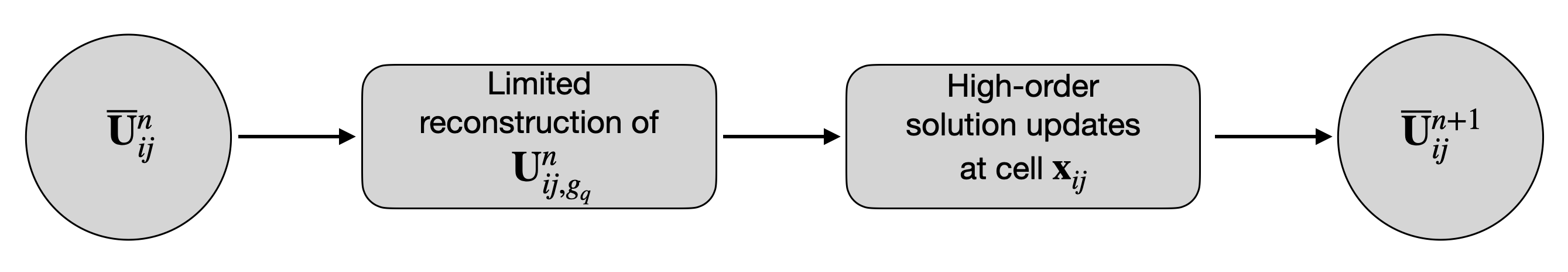
Figure 4: The logical flow line of the solution updating procedure. Shown is the principle flow line in conventional a priori high-order methods where limited spatial data reconstructions are applied to all available cells as a fundamental building-block, regardless of local flow smoothness.

For this reason, the MOOD method is considered to be an alternative paradigm that has computational benefits over the classic a priori compressible flow algorithms. This paper explores this attractive MOOD paradigm by integrating the high-order GP reconstruction methods in the MOOD framework. We emphasize that the resulting GP-MOOD method seamlessly provides the pairwise integration between the GP reconstruction methods and MOOD’s order cascading mechanism. The primary advantage of our GP-MOOD method is the performance gain and the paradigm simplification by removing the need for least-squares solves in the existing polynomial-based MOOD methods. Also will be shown are the smaller GP stencils compared to the corresponding polynomial MOOD methods at the same solution accuracy, further decreasing the computational workload and the associated memory footprint in GP-MOOD relative to the existing polynomial-based MOOD methods.

3.1 Three building blocks in GP-MOOD

The fundamental principle of the MOOD paradigm centers around three important building blocks, the detection criteria, the safe scheme, and the scheme cascade [28]. We adopt these three basic components to devise the following relaxed version for our GP-MOOD methods:

1. The detection criteria: The first component is a sequence of prescribed properties that the discrete numerical solution has to fulfill to be considered acceptable. These conditions are of two types: “Physical Admissibility Detection” (PAD) and “Numerical Admissible Detection” (NAD). In most fluid dynamics simulations, PAD ensures that the numerical solution represents an admissible flow state (e.g., positivity in pressure and density). More generally, they ensure that the numerical solution makes sense from the physical model’s point of view. They only depend on the set of PDE solved.

   On the other hand, NAD ensures that the solution produced by the solver is essentially non-oscillatory. It is based on a relaxed discrete maximum principle (DMP). It also includes the detection of non-numeric values such as NAN’s and Inf’s, that is, the admissibility of the state from a computer science point of view (Computer science Admissibility Detection or CAD). CAD is identical for all sets of PDEs. If a candidate solution does not satisfy either of the PAD and NAD criteria in some cells, such cells are recorded as troubled cells and their discrete updates are repeated with a lower order method (see (iii) below).

   Newly added to the conventional detection criteria is the so-called Compressibility-Shock Detection (CSD) check in our study. Operationally, this new condition is run after PAD and CAD (but not DMP) to measure the strengths of fluid compressibility and local shocks by measuring the local gradient of pressure ($\nabla p$) and the divergence of the velocity field ($\nabla\cdot\mathbf{V}$). We proceed to the next step of DMP only when cells undergo strong compressibility with rapid build-ups of pressure gradients. The CSD check is motivated by the early work on 1D GP reported in [54], where GP’s unlimited reconstructed solutions are used away from shocks. In contrast to the current GP-MOOD methods, the second-order limited piecewise linear method (PLM) was used where shocks are present in [54]. In this early work, local shocks were tracked by a generic shock detector [55] to selectively choose GP versus PLM depending on the local shock strengths.

   To summarize, we have the following three categories:

   • PAD: positivity preservation on density and pressure variables,

   • NAD: numerical validity that monitors CAD (NAN & Inf) and DMP (see more Section 3.3.2),

   • CSD: compressibility and shock strengths, i.e., $\nabla p>\sigma_{p}$ and $\nabla\cdot\mathbf{V}<-\sigma_{v}$, where $\sigma_{p}>0$ and $\sigma_{v}>0$ are (heuristically) tunable threshold parameters.

2. The safe scheme: The second component is the choice of a numerical method used as the last resort when all the other high order schemes have failed to produce an acceptable solution according to the detection criteria in (i). Therefore, the selection choice has to focus on scheme’s robustness and stability that guarantee to produce an admissible solution state. To this end, the first-order Godunov (FOG) scheme is most popular, while the second-order MUSCL method could be used as well to improve the results on contact discontinuity (e.g., see [57]). In this study, we use FOG for the choice of the safe scheme.

3. The scheme cascade: A family of reconstruction schemes is the third component that provides a sequential pipeline of different reconstruction methods, starting from the most accurate available method to the safe scheme. The conventional MOOD method uses a set of unlimited polynomial reconstruction methods in different orders up to the 6th-order accuracy [25, 26]. Alternatively, for the present study, we use the three unlimited linear GP reconstruction methods of 3rd-, 5th-, and 7th-order, namely, GP-R1, GP-R2, and GP-R3. As briefly introduced in Section 2.6, these GP methods and the simple 3rd-order polynomial MOOD method are used in this study.

   To summarize, we has the following four families of methods, each of which have the specific ordered cascading scheme depicted by the arrows on troubled cells:

   • the 7th-order GP-MOOD7: the cascading follows as GP-R3 $\to$ GP-R1 $\to$ FOG,

   • the 5th-order GP-MOOD5: the cascading follows as GP-R2 $\to$ GP-R1 $\to$ FOG,

   • the 3rd-order GP-MOOD3: the cascading follows as GP-R1 $\to$ FOG,

   • the 3rd-order POL-MOOD3: the cascading follows as Poly3 $\to$ FOG.

   The decrement pattern of our order-cascading within each group is consistent with the finding in [26], which simplifies the original, long-listed one-by-one polynomial degree decrement procedure (e.g., Poly 5 $\to$ Poly4 $\to$ Poly3 $\to$ Poly2 $\to$ FOG) to a shorter list of two or three methods.

The logical MOOD loop pipelines of the standard polynomial and the GP-MOOD methods are summarized and compared in Fig. 5. The primary difference between the polynomial-MOOD and GP-MOOD methods is the split of the detection criteria (the grey diamond in Fig. 5(a)) of the polynomial-MOOD method into two groups, placing PAD and CAD in the first group and the rest DMP in the second group (the two sky blue diamonds Fig. 5(b)) in the GP-MOOD loop. The newly added compressibility-shock detection check (CSD) is monitored between the two separated detection criteria groups, allowing a relaxed MOOD framework that promotes the use of GP’s high-order solution updates as much as possible.

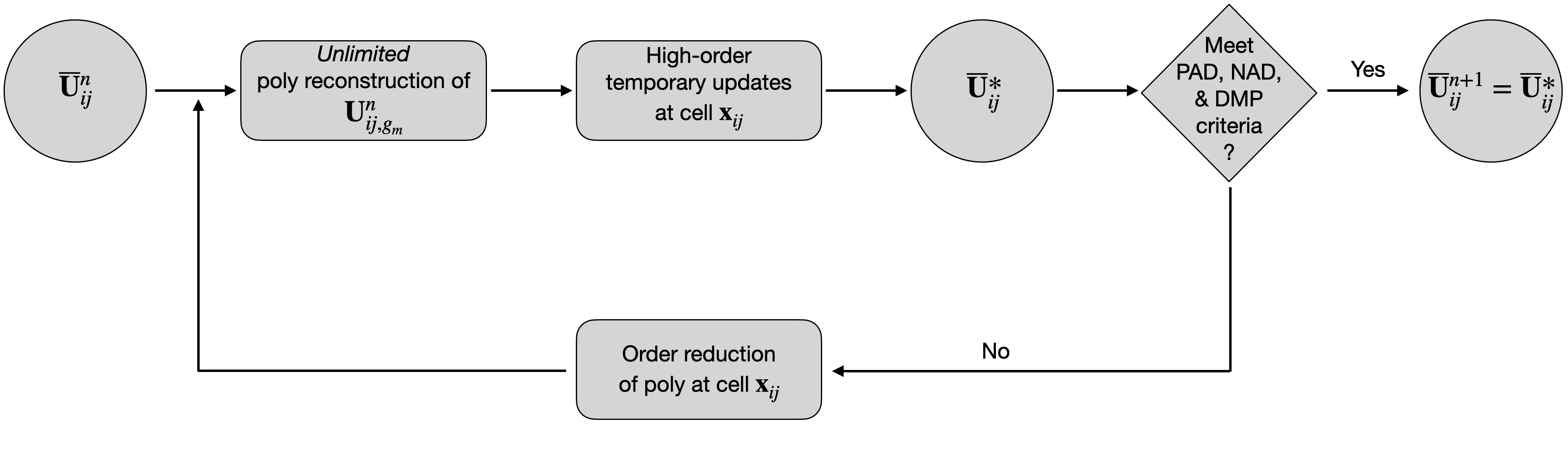
(a)

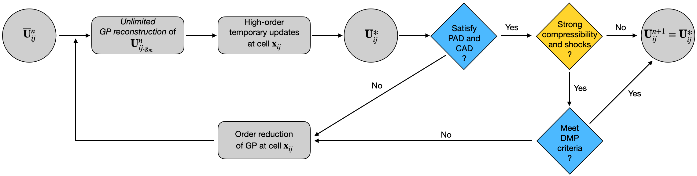
(b)

Figure 5: The logical flow of the solution updating procedure in the MOOD loop. (a) The flow chart in the existing a posteriori polynomial MOOD method. The solution accuracy of a group of unlimited polynomial data reconstruction methods cascades down from high to low until all the MOOD criteria are met in each troubled cell. (b) The flow chart of the GP-MOOD method. An extra CSD condition that checks the strength of flow compressibility (the yellow diamond) is added between the positivity and NAN & Inf check (i.e., PAD and CAD in the top sky blue diamond) and the rest MOOD criteria on DMP (the bottom sky blue diamond). The conditions in the grey diamond in Fig. 5(a) are split into the two sky blue diamonds in Fig. 5(b) for GP-MOOD. The overall order-reduction MOOD concept is relaxed with the compressibility-shock admissibility (CDS) check to maximize the use of GP’s unlimited high-order reconstructed solutions before they are reduced to lower order ones. In both, $\mathbf{U}_{ij,g_{m}}^{n}$ denotes the pointwise Riemann states at each Gaussian quadrature point, $g_{m}$, $1\leq m\leq q$, in Fig. 3; $\overline{\mathbf{U}}^{\ast}_{ij}$ denotes a volume-averaged, pre-validated candidate solution using the highest-order method available in each MOOD cascading loop.

We detail the GP-MOOD strategies described above in the next following subsections. For this paper to be self-contained, we provide concise descriptions of those existing concepts while we give sufficient details on new strategies for GP-MOOD. Interested readers refer to [24, 25, 26, 27, 28, 34] for reviewing the existing MOOD methodologies.

3.2 PAD – Physical Admissibility Detection

The PAD criterion is drawn from considering the most constitutional condition inferred from the underlying physics. As we solve the Euler equations, it is indispensable to ensure positivity in both density and pressure variables to guarantee stable discrete evolutions of numerical solutions regardless of how extreme the flow in simulations may turn into. The candidate solution $\overline{\mathbf{q}}^{*}_{ij}$ on each $\mathbf{x}_{ij}$ satisfies the PAD criterion if:

$$\overline{\rho}^{*}_{ij}>0\quad\text{and}\quad\overline{p}_{ij}^{*}>0.$$ (20)

For those cells that fail to meet this positivity condition, the solution order of accuracy gets reduced according to the decrement patterns, a) through d), described in (iii) The scheme cascade in the previous section. The logical flow repeats the MOOD loop for the next iteration.

It is important to re-emphasize that obtaining the derived primitive variable, $\overline{p}_{ij}^{*}$, from the updated conservative quantities, $\overline{\mathbf{q}}^{*}_{ij}$, involves nonlinear conversion processes such as an EoS call, which can have an impact on the solution accuracy if $\overline{p}_{ij}^{*}$ is subsequently re-used to construct any relevant conservative variables without respecting the difference between the pointwise and volume-averaged quantities. As clearly noted in Section 2.1, such a conversion is strictly prohibited. However, there is no negative impact on the solution accuracy as long as the derived pressure is used for PAD and is no longer used afterward, which is the case here.

3.3 NAD – Numerical Admissibility Detection

Below, we discuss two types of criteria that are monitored in NAD, including the CAD and the relaxed DMP criteria.

3.3.1 CAD – Computer science Admissibility Detection

The CAD criterion ensures that the updated candidate solutions $\overline{\mathbf{q}}^{*}_{ij}$ do not represent either NANs or Infs, which are direct outcomes of invalid floating-point operations, such as division by zero, square root of a negative number, arithmetics with $\pm\infty$, etc. In most hydrodynamics codes that use a priori limitings, these invalid states are considered physically violated in a strong sense because the process of a priori limitings should explicitly prohibit such states. As such, these codes are often compiled with “crash-if-NAN/Inf” flag options.

The situation is different in a posteriori MOOD paradigms, where there is no such an explicit monitoring process until a candidate solution is available, only after which invalid solutions are rejected via MOOD’s post processes. Another view to see this is that the Riemann states computed by the unlimited MOOD reconstruction are not necessarily physically valid. Indeed, those invalid states are well justified (and should be allowed) as proper outputs within the MOOD paradigm. Thus, “crash-if-NAN/Inf” compiler flags are not an option for the a posteriori MOOD-type codes. Instead, these invalid states are separately controlled via the CAD process, i.e., we say the candidate solution $\overline{\mathbf{q}}^{*}_{ij}$ satisfies the CAD criterion if:

$$\overline{\rho}^{*}_{ij}\neq(\texttt{NAN}\mbox{ or }\texttt{Inf})\quad\text{and}\quad\overline{p}_{ij}^{*}\neq(\texttt{NAN}\mbox{ or }\texttt{Inf}).$$ (21)

We also make an important note on CAD in connection to preserving the assumed symmetry in symmetry-preserving simulations. Our experiments have shown that a broken symmetry can be induced if any one of the Riemann state input pair, $(U^{n}_{L},U^{n}_{R})$ at each Gaussian quadrature point happens to be an invalid state. For example, assume that the left state vector $U^{n}_{L}$ contains several state variables that are NAN but a valid normal velocity. If the normal velocity is negative, and all the state variables in $U^{n}_{R}$ are physically valid with a negative normal velocity as well, the Riemann problem will still be able to calculate the interface flux based on the valid right states based on the upwinding nature of the Riemann problem. Since this upwind flux has been computed with such a physically non-admissible input pair, the resulting flux has no guarantee to produce a physically admissible candidate solution, albeit it qualifies all of the MOOD criteria. If this type of incident continues in simulations, this inconsistency can trigger the onset of unphysical asymmetries, which could lead to the development of erroneous flow instabilities.

To prevent this issue from happening, we check the CAD condition also on the reconstructed densities (and nonlinearly derived pressures) in all Riemann states from the high-order GP reconstruction, in addition to the updated candidate solutions at cell centers. To our knowledge, the previous studies on the MOOD methods [24, 25, 26, 27] are mostly intact from this asymmetry issue, primarily because their applications heavily focus on unstructured grid geometries where symmetry is not rigorously expected in the first place.

3.3.2 Relaxed DMP criteria: plateau + DMP + u2

The discrete maximum principle (DMP) is the crux of the MOOD method, which was single-handed to detect the solution admissibility in the original MOOD method [24]. For the exposition purposes, let us assume that we use the density variable to run the DMP check. The original DMP monitors if there is any excessive numerical oscillation produced in the resulting candidate solution $\overline{\rho}^{*}_{ij}$ at $\mathbf{x}_{ij}$ in comparison to the adjacent neighboring input states, $\overline{\rho}^{n}_{m}$,

$$\underset{m\in\mathcal{N}(ij)}{\min}\Bigl{(}\overline{\rho}_{m}^{n},\overline{\rho}_{ij}^{n}\Bigr{)}\leq\overline{\rho}_{ij}^{*}\leq\underset{m\in\mathcal{N}(ij)}{\max}\Bigl{(}\overline{\rho}_{m}^{n},\overline{\rho}_{ij}^{n}\Bigr{)},$$ (22)

where $\mathcal{N}(ij)$ is a set of all indices, including the immediate neighbors that share a common cell-face with the cell $\mathbf{x}_{ij}$. For example, in our structured 2D Cartesian grid configuration for GP-MOOD3 depicted in Fig. 1, the set $\Bigl{\{}\overline{\rho}^{n}_{m}:m\in\mathcal{N}(ij)\Bigr{\}}$ is given as $\Bigl{\{}\overline{\rho}^{n}_{m}:m=2,3,4,5\Bigr{\}}$. This concept is extended to the following DMP check for a $p$-stage RK method,

$$\underset{m\in\mathcal{N}(ij)}{\min}\Bigl{(}\overline{\rho}_{m}^{n,rk(s)},\overline{\rho}_{ij}^{n,rk(s)}\Bigr{)}\leq\overline{\rho}_{ij}^{*,rk(s)}\leq\underset{m\in\mathcal{N}(ij)}{\max}\Bigl{(}\overline{\rho}_{m}^{n,rk(s)},\overline{\rho}_{ij}^{n,rk(s)}\Bigr{)},\quad\text{for each }1\leq s\leq p,$$ (23)

where $\overline{\rho}_{m}^{n,rk(s)}$ and $\overline{\rho}_{ij}^{*,rk(s)}$ are respectively the adjacent initial states and the resulting candidate solution at each stage $s$ over the course of the $p$-stage RK updates.

In the follow-up studies [25, 26, 27, 28], this single-handed DMP criterion has been further revised and relaxed by two additional detections, namely the Plateau detection and the u2 detection. Hereunder, we describe them briefly in the order they are used during the NAD procedure. Following [28], the Plateau detection is executed before the original DMP in Eq. 23 in order to avoid the loss of precision on constant flat plateau states as a consequence of the criterion in Eq. 23 that detects not only large unphysical oscillations but also micro-oscillations. To improve such situations, the first relaxation takes place in the form of skipping the DMP criterion in Eq. 23 if micro-oscillations (hence the name Plateau detection) are present:

$$\underset{m\in\mathcal{N}(ij)}{\max}\Bigl{(}\overline{\rho}_{m}^{n,rk(s)},\overline{\rho}_{ij}^{n,rk(s)}\Bigr{)}-\underset{m\in\mathcal{N}(ij)}{\min}\Bigl{(}\overline{\rho}_{m}^{n,rk(s)},\overline{\rho}_{ij}^{n,rk(s)}\Bigr{)}<\min(\Delta x^{3},\Delta y^{3}).$$ (24)

The second relaxation called the u2 detection aligns with overcoming the second-order-accuracy bottleneck if the MOOD loop strictly satisfies the original DMP in Eq. 23 [26]. A resolution is made available by allowing the violation of Eq. 23 on smooth extrema via the u2 detection. Executed after Eq. 23, the u2 detection reinstates the admissibility of the rejected candidate solutions from Eq. 23. The u2 detection checks if the rejection is the consequence of the situation where a new extremum state $\overline{\rho}_{ij}^{*,rk(s)}$ happens to be present in the region where local flows experience smooth variations. If this is the case, the rejection is revoked, and its admissibility is reinstated. To meet this, u2 calculates local second derivative quantities to measure local curvatures,

$$\mathcal{C}_{d,ij}^{\min}=\underset{m\in\mathcal{N}(ij)\cup\{ij\}}{\min}\left(\frac{\partial^{2}\overline{\rho}_{m}^{n,rk(s)}}{\partial{\eta^{2}}}\right)\;\;\text{, }\quad\mathcal{C}_{d,ij}^{\max}=\underset{m\in\mathcal{N}(ij)\cup\{ij\}}{\max}\left(\frac{\partial^{2}\overline{\rho}_{m}^{n,rk(s)}}{\partial{\eta^{2}}}\right),\quad\text{for each }1\leq s\leq p,$$ (25)

where $\eta=\mathbf{e}_{d}\cdot\mathbf{x}$ denotes each of $x,y,$ respectively for each $d=x,y$. With these curvatures, a candidate solution $\overline{\mathbf{q}}_{ij}^{*,rk(s)}$ rejected by Eq. 23 after the $s$th RK substage update, nonetheless regains its admissibility if the initial states $\overline{\rho}_{m}^{n,rk(s)}$ at each $s$th RK stage fall on a smooth extrema region, checked by either of the followings:

$$\mathcal{C}_{d,ij}^{\min}\mathcal{C}_{d,ij}^{\max}>-\delta\;\;\mbox{ and }\;\;\max\Biggl{(}\Big{|}\mathcal{C}_{d,ij}^{\max}\Big{|},\Big{|}\mathcal{C}_{dir,ij}^{\min}\Big{|}\Biggr{)}<\delta,$$ (26)

or

$$\mathcal{C}_{d,ij}^{\min}\mathcal{C}_{d,ij}^{\max}>-\delta\;\;\mbox{ and }\;\;\frac{\Big{|}\mathcal{C}_{d,ij}^{\min}\Big{|}}{\Big{|}\mathcal{C}_{d,ij}^{\max}\Big{|}}\geq\frac{1}{2},$$ (27)

for all $d=x,y$ with $\delta=\min\{\Delta x,\Delta y\}$. One can use the standard centered differencing for the second partial derivatives in Eq. 25. To provide another application of GP, we instead use a new second-derivative GP formula that can be derived by taking second derivatives of the GP prediction vector, $\mathbf{t}_{*}$, in Eq. 14. We show its derivation in B.

3.4 CSD – Compressibility-Shock Detection

As shown in Fig. 5(b), an extra layer called CSD is added to the MOOD loop between the PAD/CAD checks and the relaxed DMP check in order to early-accept a candidate solution as the final high-order solution without DMP if the candidate solution does not reside inside a strong shock. A multidimensional shock detection switch is employed for this purpose. Following  [56], a candidate solution $\overline{\mathbf{q}}^{*,rk(s)}_{ij}$ is recorded as valid and exits the MOOD loop if the local flow is weakly compressible,

$$\nabla\cdot\overline{\mathbf{V}}_{ij}^{n,rk(s)}\equiv\frac{\overline{u}_{i+1,j}^{n,rk(s)}-\overline{u}_{i-1,j}^{n,rk(s)}}{2\Delta x}+\frac{\overline{v}_{i,j+1}^{n,rk(s)}-\overline{v}_{i,j-1}^{n,rk(s)}}{2\Delta y}\geq-\sigma_{v}$$ (28)

and the local (normalized) pressure gradient is weak,

$$\widetilde{\nabla}\overline{p}_{ij}^{n,rk(s)}\equiv\frac{\Big{|}\overline{p}_{i+1,j}^{n,rk(s)}-\overline{p}_{i-1,j}^{n,rk(s)}\Big{|}}{2\Delta x\min\{\overline{p}_{i+1,j}^{n,rk(s)},\overline{p}_{i-1,j}^{n,rk(s)}\}}+\frac{\Big{|}\overline{p}_{i,j+1}^{n,rk(s)}-\overline{p}_{i,j-1}^{n,rk(s)}\Big{|}}{2\Delta y\min\{\overline{p}_{i,j+1}^{n,rk(s)},\overline{p}_{i,j-1}^{n,rk(s)}\}}\leq\sigma_{p},$$ (29)

where $\sigma_{v}$ and $\sigma_{p}$ are both positive tunable parameters. Similar to [56], our default choice is heuristically set to 5 for both, which sufficiently and satisfactorily reroutes candidate solutions to early acceptance at each $s$th RK sub-stage according to the two conditions in Eqs. 28 and 29, promoting the use of GP’s high-order solutions without further order decrement.

We have observed that this new CSD criterion is necessary to control numerical dissipation on the right scale. Otherwise, the final validated solutions channeled directly to the next DMP check without early acceptance become too diffusive to trigger subsequent nonlinear flow patterns that have been well-understood as unique signatures of such benchmark problems. Examples are discussed in Sections 5.2.1 and 5.2.4.

3.5 The safe scheme

The first order Godunov (FOG) scheme is our choice for “the safe scheme” to guarantee the inherent solution robustness with strong positivity preservation if all tried high-order solutions turn out to be inadmissible during the MOOD loop. As will be seen in Section 5, the FOG solutions are employed near shocks and discontinuities in most shock dominant simulations, taking less than 10% of the entire domain in practice. Another possible choice could be to use a limited 2nd-order TVD linear method as a safe scheme to improve the solution quality around contact discontinuities with extra care for positivity preservation (e.g., see [57]). However, compared to the safe scheme with FOG, this choice could potentially compromise the strong positivity preservation as well as the rest desirable properties monitored in the MOOD loop since those properties are no longer to be checked once the solution cascades down to the safe scheme but to admit it.

3.6 The scheme cascade with GP

In GP-MOOD, the original strategy in polynomial-based MOOD methods with polynomial reconstruction schemes, their grouping, and the order decrement in the MOOD loop are replaced by the GP alternatives of high-order unlimited linear GP reconstruction with different choices of $R=1,2,3$. Three GP groups for the MOOD cascade, introduced in Section 3.1, are our GP alternatives to the polynomial-based MOOD methods. They are the 7th-order GP-MOOD7 (GP-R3 $\to$ GP-R1 $\to$ FOG), the 5th-order GP-MOOD5 (GP-R2 $\to$ GP-R1 $\to$ FOG), and the 3rd-order GP-MOOD3 (GP-R1 $\to$ FOG) for GP-MOOD. The additional 3rd-order POL-MOOD3 (Poly3 $\to$ FOG) will be used for comparison.

In [24], three systematic strategies called EdgePD have been introduced. The main idea is to provide a consistent way to assign a specific choice of reconstruction order of accuracy at each cell face when the two neighboring cells that share the cell face in common are at different orders or accuracy as a result of different paths in the MOOD order decrement.

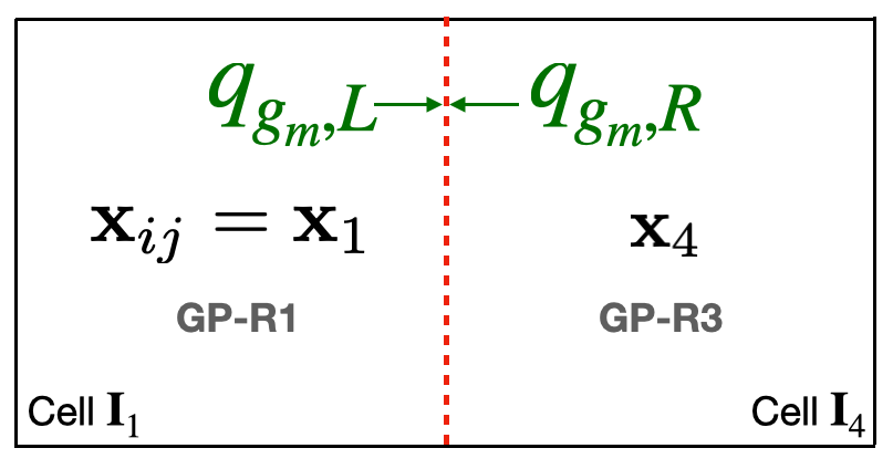
Figure 6: A GP-MOOD7 example for determining reconstruction orders for two Riemann states, $q_{g_{m},L}$ and $q_{g_{m},R}$, which respectively belong to the cell $\mathbf{I}_{1}$ on the left and $\mathbf{I}_{4}$ on the right. The Riemann states are displayed at one of the Gaussian quadrature points, $g_{m}$, $m=1,\dots,q$, on the cell face $\mathbf{x}_{i+1/2,j}=(x_{i+1/2},y_{j})$ (red dotted line) for the $q$-point Gaussian quadrature rule. In this example with GP-MOOD7, we specifically use the 4-point quadrature rule (i.e., $q=4$) that provides the 8th-order quadrature rule, sufficient for the 7th-order GP-MOOD7.

For example, assume that the computation is being done with the 7th-order GP-MOOD7, which is integrated with the 4-point Gaussian quadrature rule (i.e., $q=4$, see Fig. 3). Consider a situation in Fig. 6, where the cell face at $(x_{i+1/2},y_{j})$ is depicted in a red dotted line. Two cells that share this face, namely $\mathbf{I}_{1}$ and $\mathbf{I}_{4}$, are centered at $\mathbf{x}_{1}=(x_{i},y_{j})$ and $\mathbf{x}_{4}=(x_{i+1},y_{j})$, respectively. Readers can see that these two cells are extracted from Fig. 2(b). What can happen is that, at any $s$th RK sub-stage, the reconstruction order at $\mathbf{I}_{4}$ remains at the highest 7th-order with GP-R3 while it has been reduced to the 3rd-order with GP-R1 on $\mathbf{I}_{1}$. There are three different ways to assign a reconstruction order at each of the left and right Riemann state pair $(q_{g_{m},L},q_{g_{m},R})$ at each Gaussian quadrature point, $g_{m}$. See also Fig. 3. The first option called $\mbox{EDP}_{0}$ is to assign the Riemann state that belongs to each of the cells the same order each cell is at. That is, GP-R1 is assigned to $q_{g_{m},L}$ while GP-R3 to $q_{g_{m},R}$. The second option, $\mbox{EDP}_{1}$, takes the minimum of the two, GP-R1 and GP-R3, and assigns the minimum to both, i.e., GP-R1 is assigned to both $q_{g_{m},L}$ and $q_{g_{m},R}$. The last option, $\mbox{EDP}_{2}$, considers other three neighboring cells around $\mathbf{x}_{1}$ as well (e.g., they are $\mathbf{I}_{2},\mathbf{I}_{3}$, and $\mathbf{I}_{5}$ in Fig. 2(b)) and extend the minimum search to these cells to assign the resulting minimum order to all 16 Riemann states (i.e., four faces times four Riemann states per face) that belong to $\mathbf{I}_{1}$. The study in [24] points out that $\mbox{EDP}_{0}$ should not be used to properly exit the MOOD loop within a finite number of cascades; hence it is not our choice. On the other hand, $\mbox{EDP}_{2}$ is more aggressive than $\mbox{EDP}_{1}$ in reducing the reconstruction order at the cell under consideration. For this reason, our choice for GP-MOOD is $\mbox{EDP}_{1}$ in this study.

3.7 Quick summary of the GP-MOOD procedures

Putting all things together, we summarize the GP-MOOD procedures in Fig. 7, focusing on the individual detection criterion at each stage. Fig. 5(b) (the top portion) is revisited in Fig. 7 to map to the corresponding sub-steps (the bottom portion).

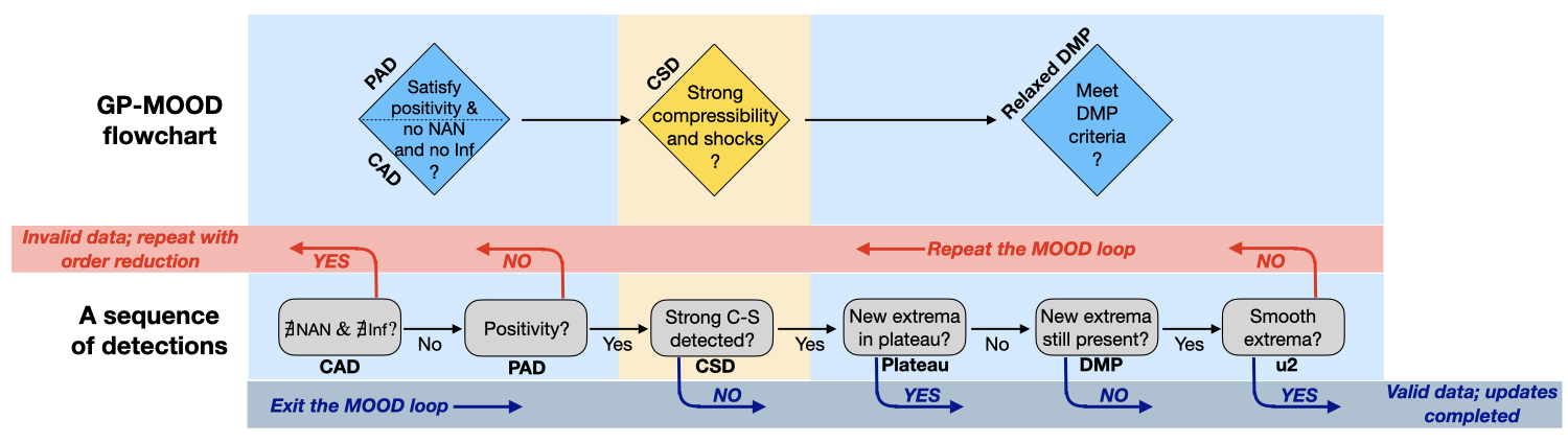
Figure 7: Flowchart of the detection at each sub-step used in the GP-MOOD loop. The sub-steps in the bottom portion with “A sequence of detections” belong to the corresponding steps in the top portion with “GP-MOOD flowchart.” Accordingly, the candidate solutions are rerouted from each of those sub-steps to either the next MOOD loop (invalid data on the red horizontal stripe in the middle) or the exit of the MOOD loop (valid data on the grey-blue horizontal stripe in the bottom). All criteria except for PAD and CSD belong to NAD.

3.8 Time integration

To achieve the anticipated target solution accuracy at 3rd-, 5th-, and 7th-order in GP-MOOD, it is necessary that the consideration of temporal accuracy also needs to be accounted for correspondingly. Any simulations that are integrated with a temporal solver, whose accuracy is lower than the spatial solver, will be penalized by the lower temporal accuracy. The situation is easily understood when a $p$th order spatial method is integrated with a $q$th order temporal solver. The error in discrete updates will be dominated by the leading error determined by either of the two cases, $\mathcal{O}(\Delta s^{p})>\mathcal{O}(\Delta t^{q})$ or $\mathcal{O}(\Delta s^{p})<\mathcal{O}(\Delta t^{q})$ with $\Delta s=\min\{\Delta x,\Delta y,\Delta z\}$ in 3D generally. Two recent studies by Lee et al.  [58, 59] have shown that, in the case with the lower order temporal method, $q<p$, there exist a critical grid delta $\Delta s_{\text{crit}}$ beyond which (i.e., the grid delta $\Delta s$ becomes smaller than $\Delta s_{\text{crit}}$) the numerical error is severely penalized and follow the convergence rate dictated by the lower temporal accuracy. In numerical simulations, this temporal error dominance becomes more influential at high resolutions, creating a computational dilemma of not making the expected solution improvements by refining spatial grids.

As such, our strategy is to employ SSP-RK solvers and match temporal accuracy with GP’s spatial accuracy in all our convergence studies on smooth flows. In other shock dominant simulations, where a rigorous convergence rate can be lifted, we choose a relevant SSP-RK solver whose accuracy may be lower than the spatial GP solvers to reduce the computational cost.

Two choices of our SSP-RK solvers include the optimal three-stage, 3rd-order SSP-RK3 solver  [8, 41] given as (we drop the cell index $ij$ for simplicity),

$$\overline{\mathbf{U}}^{n+1}=\frac{\overline{\mathbf{U}}^{n}+2\overline{\mathbf{U}}^{(3)}}{3},\;\;\text{ where }\;\;\;\begin{cases}\overline{\mathbf{U}}^{(1)}=\overline{\mathbf{U}}^{n}\ -\Delta t\,\mathbb{F}_{\nabla}(\overline{\mathbf{U}}^{n}),\\ \overline{\mathbf{U}}^{(2)}=\overline{\mathbf{U}}^{(1)}-\Delta t\,\mathbb{F}_{\nabla}(\overline{\mathbf{U}}^{(1)}),\\ \overline{\mathbf{U}}^{(3)}=\hat{{\mathbf{U}}}^{(2)}-\Delta t\,\mathbb{F}_{\nabla}(\hat{{\mathbf{U}}}^{(2)})\;\mbox{ with }\;\hat{{\mathbf{U}}}^{(2)}=\frac{1}{4}(3\overline{\mathbf{U}}^{n}+\overline{\mathbf{U}}^{(2)}),\\ \end{cases}$$ (30)

and the optimal five-stage 4th-order SSP-RK4 solver [42],

$$\begin{aligned} \overline{\mathbf{U}}^{n+1}&=0.517231671970585\,\overline{\mathbf{U}}^{(2)}\\ &+0.096059710526147\,\overline{\mathbf{U}}^{(3)}+0.063692468666290\,\Delta t\,\mathbb{F}_{\nabla}(\overline{\mathbf{U}}^{(3)})\\ &+0.386708617503269\,\overline{\mathbf{U}}^{(4)}-0.226007483236906\,\Delta t\,\mathbb{F}_{\nabla}(\overline{\mathbf{U}}^{(4)}),\end{aligned}$$ (31)

where the intermediate solutions at each sub-step are given as

$$\begin{cases}\overline{\mathbf{U}}^{(1)}=\overline{\mathbf{U}}^{n}-0.391752226571890\,\Delta t\,\mathbb{F}_{\nabla}(\overline{\mathbf{U}}^{n}),\\ \overline{\mathbf{U}}^{(2)}=0.444370493651235\,\overline{\mathbf{U}}^{n}+0.555629506348765\,\overline{\mathbf{U}}^{(1)}-0.368410593050371\,\Delta t\,\mathbb{F}_{\nabla}(\overline{\mathbf{U}}^{(1)}),\\ \overline{\mathbf{U}}^{(3)}=0.620101851488403\,\overline{\mathbf{U}}^{n}+0.379898148511597\,\overline{\mathbf{U}}^{(2)}-0.251891774271694\,\Delta t\,\mathbb{F}_{\nabla}(\overline{\mathbf{U}}^{(2)}),\\ \overline{\mathbf{U}}^{(4)}=0.178079954393132\,\overline{\mathbf{U}}^{n}+0.821920045606868\,\overline{\mathbf{U}}^{(3)}-0.544974750228521\,\Delta t\,\mathbb{F}_{\nabla}(\overline{\mathbf{U}}^{(3)}).\end{cases}$$ (32)

The SSP property ensures that if each sub-step solution is admissible, so is the final updated solution $\overline{\mathbf{U}}^{n+1}_{ij}$.

3.9 Numerical stability and performance comparison

For the simulations reported in this paper, we find empirically that the GP-MOOD methods are readily stable up to a CFL number of 0.8. This stability limit is larger than the theoretical limits of the above SSP-RK methods set by the so-called CFL coefficient $\mathcal{C}$ (e.g., [42]) (or also known as the SSP coefficient, e.g., [60]), with which the stable time step is defined as $\Delta t=\mathcal{C}\Delta t_{\mbox{\tiny{FE}}}$. The stability theory prescribes that $\mathcal{C}=1/D$ for SSP-RK3 in Eq. (30) and $\mathcal{C}=1.508/D$ for SSP-RK4 in Eq. (31), where $D$ is the spatial dimensionality of each problem. As pointed out in [60], $\mathcal{C}$ depends solely on time discretization, and the first-order accurate Forward-Euler time step $\Delta t_{\mbox{\tiny{FE}}}$ depends solely on spatial discretization. In our MOOD approach, the dependency of $\Delta t_{\mbox{\tiny{FE}}}$ is related to all participating high-order GP methods as well as FOG. The a posteriori nature of the MOOD order cascading algorithm makes it hard to perform a formal theoretical stability analysis of our methods. As such, we instead conduct a numerical test to determine the numerical stability bound of our methods empirically.

To see this, we set up a 2D Sedov problem (see Section 5.2.2) on a $400\times 400$ grid resolution and monitor the stability of a baseline model chosen for the stability test purpose. The choice of our baseline model consists of the 3rd-order setting, namely GP-MOOD3 and SSP-RK3, solved with the HLLC Riemann solver. The 4th-order accurate two-point quadrature rule is used by default for the 3rd-order setting. Besides, we tested our baseline model with the 2nd-order one-point quadrature rule to illustrate the stability sensitivity to different quadrature rules. Lastly, we compare our baseline model to the FOG-only model with one-point quadrature to help provide the stability gain afforded by the 3rd-order GP solution in GP-MOOD3. Note that, for FOG, the use of the two-point (and other multi-point) quadrature rule is identical to the use of the one-point quadrature rule since each volume-averaged quantity is constant on each cell.

Let us first realize that there are a couple of typical signatures when a numerical method becomes unstable. They include the presence of checkerboard patterns (or odd-even decoupling) that appear due to the lack of numerical stability used in a simulation; unphysical oscillations near shocks and discontinuities, which grow rapidly in time. The former issue can be cured by imposing added numerical dissipation, which can be alleviated by switching to a more diffusive reconstruction method or a Riemann solver, adding multidimensional wave information, or reducing a CFL number. Similarly, the latter situation can also be improved by adopting a more limited reconstruction (irrelevant for GP-MOOD), a more diffusive Riemann solver, or reducing a CFL number. In our GP-MOOD methods, we expect solutions to evolve with unlimited high-order GP methods as long as numerical stability is sufficiently provided, except at shocks and discontinuities where FOG is to be chosen as the last resort after all unlimited high-order GP solutions (should) fail there.

Based on these considerations, we grant a method is numerically stable if the method satisfies the following criteria: (i) there is no checkerboard pattern, particularly in the low dense central region (see Fig. 8), (ii) there is no unphysical growth of variables in magnitude, (iii) there is no crash caused by NAN or Inf, (iv) there is no FOG solution present in the smooth central region, i.e., the unlimited 3rd-order GP solver successfully produced stable solutions in the central region (see the right panel in Fig. 8), and finally (v) the Sedov explosion retains self-similar and symmetry.

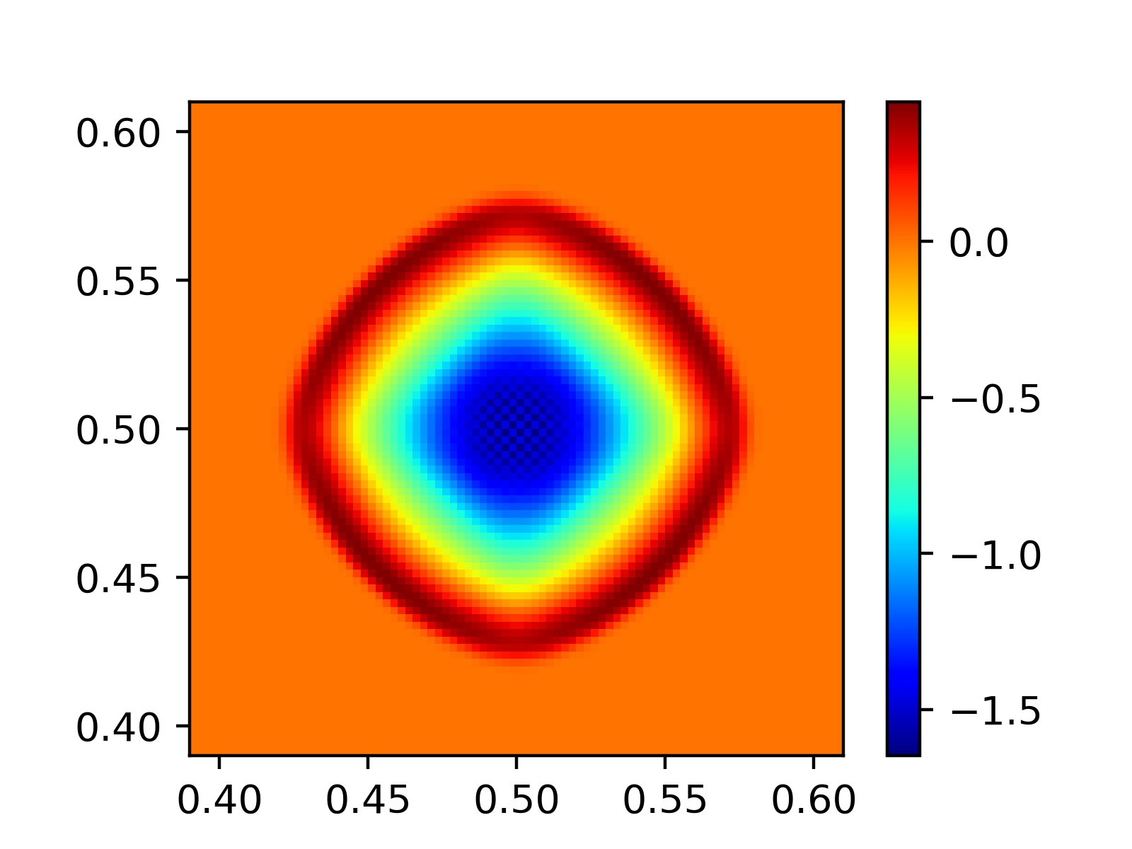
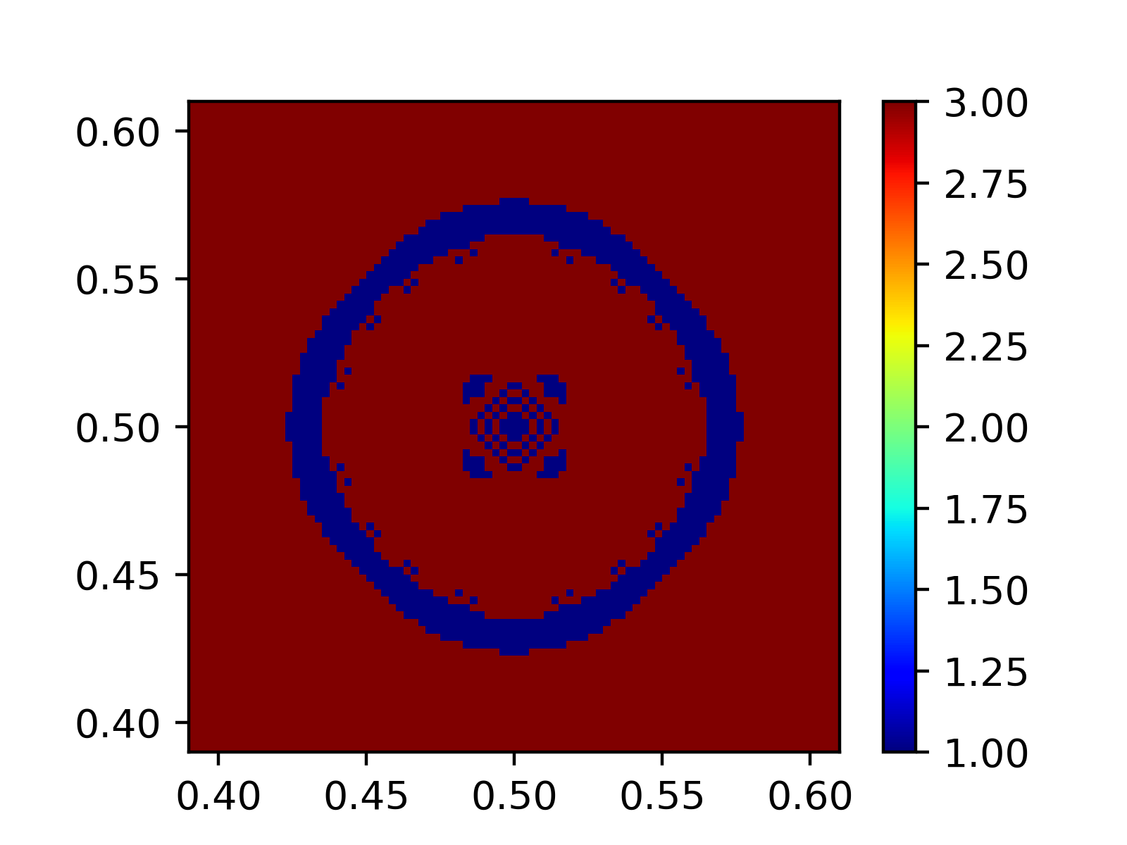
Figure 8: Examples of unstable runs of the Sedov explosion problem. (left) A checkerboard pattern appears in the central low-density region due to insufficient numerical stability in the simulation, configured with the FOG-only model using CFL=0.8. The plot displays the zoomed-in density at $t=5.5225\times 10^{-3}$. The checkerboard pattern grows in time and eventually leads the run to crash. (right) Another unstable run using the baseline model with 1-point QR and CFL=0.85. The solution order distribution (i.e., either “1” or “3” to display the local regions of the flow corresponding to the solutions with FOG and GP-R1, respectively) is plotted at $t=3.9044\times 10^{-3}$. The FOG solutions (dark blue) are present not only at shocks but also in the low-dense, smooth central region, the latter of which is related to a checkerboard-patterned density formation (not shown) similar to the left panel.

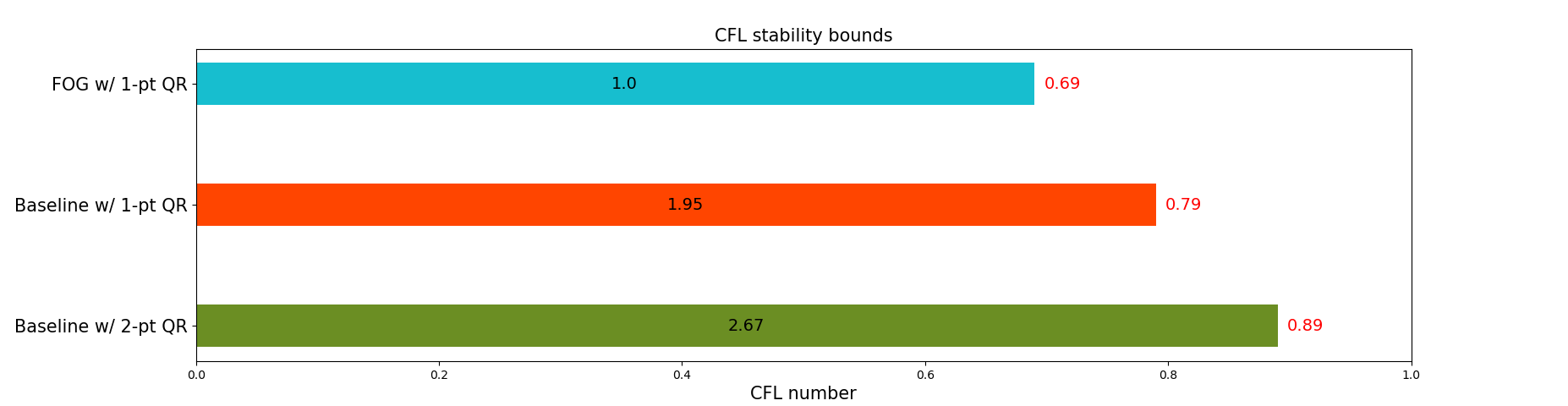
Figure 9: Empirical CFL stability bounds for GP-MOOD3 and FOG. The baseline model is the combination of GP-MOOD3 with HLLC and SSP-RK3. The FOG-only model (top) is solved using 1-point quadrature rule (QR), while the baseline models are solved using 1-point (middle) and 2-point (bottom) QRs to test the 2D Sedov problem resolved on a $400\times 400$ grid resolution. The numbers in black labeled on each bar graph represent the CPU performance for each corresponding CFL bound, normalized by the CPU performance of the FOG-only model (top). The numbers in red next to each bar are the empirical CFL bounds that ensure numerical stability in each test case. The performance results are the average of five independent runs using non-parallel, serial calculations on a 2.4 GHz 8-Core Intel Core i9 CPU.

The results are displayed in Fig. 9. The FOG-only model is shown to be stable up to CFL=0.69, beyond which the central region exhibits severe checkerboard patterns, leading to crash. This odd-even decoupling in the central region is significantly improved using the multidimensional 3rd-order GP-R1, which gains more stability by adding wave information from each transverse direction. As a result, the CFL stability bound grows from CFL=0.69 with FOG-only to CFL=0.79 with the baseline model with the 1-point quadrature rule (QR). Doubling the number of quadrature points to the 2-point QR further enhances the CFL bounds to CFL=0.89 with the baseline model. We also measured the CPU performance of the time-to-solution in each model, respectively, with CFL=0.69, 0.79, and 0.89. Normalized by the FOG-only model, the baseline run with the 1-point QR is 1.95 times more expensive than FOG-only, while the ratio becomes 2.67 for the baseline run with the 2-point QR. In addition, the baseline run with the 2-point QR and CFL=0.89 (the bottom dark green bar in Fig. 9) is 1.37 times more expensive than the baseline run with the 1-point QR and CFL=0.79 (the middle red bar in Fig. 9). On the other hand, the CPU performance ratio at CFL=0.69 of the baseline model with the 1-point QR (not shown) to the FOG-only model (the top cyan bar in Fig. 9) is observed to be 2.07, while the ratio at CFL=0.79 of the baseline model with 2-point QR (not shown) to the baseline model with the 1-point QR (the middle red bar in Fig. 9) is 1.60.

Note that the baseline model with the 2-point QR (the bottom dark green bar in Fig. 9) is the least stable option among the test cases in Section 5. From the results herein, we conclude that the GP-MOOD methods studied in this paper are sufficiently stable with CFL = 0.8; hence is the default choice in Section 5. In all stable GP-MOOD3 runs tested in this section, the percentage of those cells solved by FOG as the result of MOOD’s order reduction never exceeds 2% of the entire cells, leaving about 98% of the domain solved by the unlimited 3rd-order GP method. This fact can also be viewed as an algorithmic efficacy of GP-MOOD’s a posteriori approach over the classical a priori paradigm, where, in the latter, the use of computationally intensive nonlinear limiters is required to be always fully activated and calculated on all cells for stability. This experiment indicates that the nonlinear limiters are not required on 98% of them. Such an unnecessary computation is efficiently circumvented in GP-MOOD.

4 Stepwise implementation of the GP-MOOD method

In this section, we summarize the GP-MOOD method proposed in this study in a stepwise fashion. We intend to provide a bird-eye view of GP-MOOD for ease of practical implementation.

1. Step 1: Choose a hyperparameter, $\ell$, for each simulation. We recommend a constant value (see Section 5.1) for a convergence study while our default choice $\ell=6\Delta$ or $\ell=12\Delta$ with $\Delta=\min\{\Delta x,\Delta y\}$ works well for most of the problems in  Section 5.

2. Step 2: Once a grid is configured, calculate the GP covariance kernels in Eqs. 11 and 2.4 and compute the GP prediction vector $\mathbf{z}_{*}^{T}$ according to  Eqs. 14 and 15 for $R=1$ with the chosen $\ell$. Save the computed $\mathbf{z}_{*}^{T}$ for later use. Repeat the same for $R=2$ if GP-MOOD5 is considered. Instead, repeat the same for $R=3$ if GP-MOOD7 is considered. Group these GP methods according to the GP-MOOD3, GP-MOOD5, and GP-MOOD7 cascading families alongside FOG.

3. Step 3: Start a simulation. The 3rd-order GP-R1 is solved with the 2-point quadrature rule; the 5th-order GP-R2 with the 3-point rule; the 7th-order GP-R3 with the 4-point rule. Choose a proper SSP-RK method. After each $s$th RK sub-stage at $n$th timestep, each of the procedures in the MOOD loop in Fig. 5(b) will be tested on the $s$th candidate solution, $\overline{\mathbf{U}}^{*,rk(s)}_{ij}$.

4. Step 4: Execute the CAD criteria in Eq. 21. If there are no NAN’s and no Inf’s, the solution moves to Step 5; otherwise, record the solution as inadmissible and conduct the MOOD order reduction. Repeat the MOOD loop with the next accurate reconstruction method starting from Step 4.

5. Step 5: Execute the PAD criteria in Eq. 20. If the candidate solution passes PAD, go to Step 6; otherwise, record the solution as inadmissible and conduct the MOOD order reduction. Repeat the MOOD loop with the next accurate reconstruction method starting from Step 4. Note that the order of operations between Step 4 and Step 5 can be swapped.

6. Step 6: Run the CSD criteria in Eqs. 28 and 29. If there are no strong compression and no strong pressure gradients in the local gas, record the candidate solution as admissible and accept it as the final solution. Finish the MOOD loop. Otherwise, go to Step 7.

7. Step 7: Check the Plateau criterion in Eq. 24. If the solution satisfies Eq. 24, record the candidate solution as admissible and take it as the final solution. Finish the MOOD loop. Otherwise, go to Step 8.

8. Step 8: Check DMP in Eq. 23. If the solution satisfies Eq. 23, record it as admissible and take it as the final solution. Exit the MOOD loop. Otherwise, go to Step 9.

9. Step 9: Run the u2 checks in Eqs. 25, 26 and 27 as the last MOOD test. If the candidate solution meets either Eq. 26 or  Eq. 27, take it as the final admissible solution and exit the MOOD loop. Otherwise, conduct the MOOD order reduction by one cascade. Repeat the MOOD loop with the next accurate reconstruction method starting from Step 4.

10. Step 10: Once the MOOD loop reaches the safe method, FOG, take it as the final admissible solution. Exit the MOOD loop. No further MOOD check is needed at this point.

The entire GP-MOOD pipeline is pictured as a flowchart in Fig. 5(b), while a zoomed-in view that focuses more on the MOOD criteria is schematically provided in Fig. 7.

5 Numerical results

This section displays three types of test problems, including

• a grid convergence test problem in 2D that assesses the accuracy of the proposed GP-MOOD methods (see Section 5.1),

• standard shock-dominant benchmark problems in 1D and 2D that test the validity of our GP-MOOD solvers on a set of well-known CFD problems (see Section 5.2), and finally,

• highly compressible, strong shock problems that are known as stringent for numerical testing purposes. These problems require a strong positivity-handling and expensive nonlinear shock-limiters in the a priori FV literature (see Section 5.3).

The choice of a Riemann solver is default to be the HLLC Riemann solver [61] in all test problems, except that the HLL Riemann solver [62] is used for the last two test problems in Section 5.3 to suppress the grid-aligned carbuncle instabilities [63]. For GP, we follow  [20, 21] to set $\ell=1$ for the 2D convergence test problem in Section 5.1 and $\ell=6\Delta$ for the 1D Shu-Osher shock tube problem in Section 5.2.1, while we set $\ell=12\Delta$ in all other problems in this section. As discussed in Section 3.9, we take a CFL number of 0.8 by default. The ratio of specific heats is set to be $\gamma=1.4$ in all test problems.

5.1 Grid convergence – The isentropic vortex test

The accuracy of the GP-MOOD schemes is considered on a well-known 2D test problem called the nonlinear isentropic vortex advection presented by Shu [64]. As in [21] we double the original domain size to avoid self-interactions of the vortex across the periodic domain. It sets up a circular region centered at $(x_{c},y_{c})=(10,10)$ on a periodic square domain, $[0,20]\times[0,20]$, where a Gaussian-shaped vortex with rotating velocity fields are initialized. As the problem consists of the smooth advection of the vortex along the diagonal direction, any departure from the initial condition (or the exact solution of the problem) will be considered numerical errors of the numerical method under consideration.

We follow the standard initial condition in [64] to initialize pointwise values of the primitive variables as

$$\rho(x,y) = \left[1-\left(\gamma-1\right)\frac{\beta^{2}}{8\gamma\pi^{2}}e^{1-r^{2}}\right]^{\frac{1}{\gamma-1}},$$ (33)

$$u(x,y) = 1-\frac{\beta}{2\pi}e^{\frac{1}{2}\left(1-r^{2}\right)}(y-y_{c}),$$ (34)

$$v(x,y) = 1+\frac{\beta}{2\pi}e^{\frac{1}{2}\left(1-r^{2}\right)}(x-x_{c}),$$ (35)

$$p(x,y) = \rho(x,y)^{\gamma},$$ (36)

with $r=r(x,y)=\sqrt{(x-x_{c})^{2}+(y-y_{c})^{2}}$ and the vortex strength $\beta=5.$ With the mean diagonal flow velocity fields, $(u,v)=(1,1)$, the vortex makes one period of diagonal advection and returns to the initial position at $t_{\tiny{\max}}=20,$ at which point we measure numerical errors.

For a successful error analysis, it is crucial to convert these pointwise values to the volume-averaged conservative quantities – the data type evolved in FV – to ensure that there is no accuracy loss in FV evolutions. If one initializes conservative quantities with the pointwise values without converting to volume-averaged quantities, the simulation will introduce an error of order two (i.e., $\mathcal{O}(\Delta x^{2}+\Delta y^{2})$) right at the initial step even before any solution evolution. This initial error will deter us from assessing the correct convergence rates of our GP-MOOD methods. This concern was clearly pointed out in our earlier discussion, (i), (ii), and (iii) in Section 2.1. To this end, we perform the followings:

1. We convert the pointwise primitive variables (i.e., the initial conditions in Eq. (33) – Eq. (36)) to the corresponding pointwise conservative variables and use a sufficiently highly accurate quadrature rule to convert them to the corresponding volume-averaged conservative quantities. We use the 10th-order accurate 5-point Gauss-Legendre quadrature for the conversion to guarantee that the initial setup accuracy is much higher than all of the rest discrete operations in the simulation.

2. To match the temporal accuracy of SSP-RK3 and SSP-RK4 with those of GP’s spatial accuracy, we further reduce time steps $\Delta t$ so that the temporal error is scaled down to (or smaller than or equal to) the spatial error. For example, the time step size of SSP-RK4 is scaled as constant according to $\Delta t=\Delta^{\frac{5}{4}}$, $\Delta=\min\{\Delta x,\Delta y\}$, when used with the 5th-order GP-MOOD5.

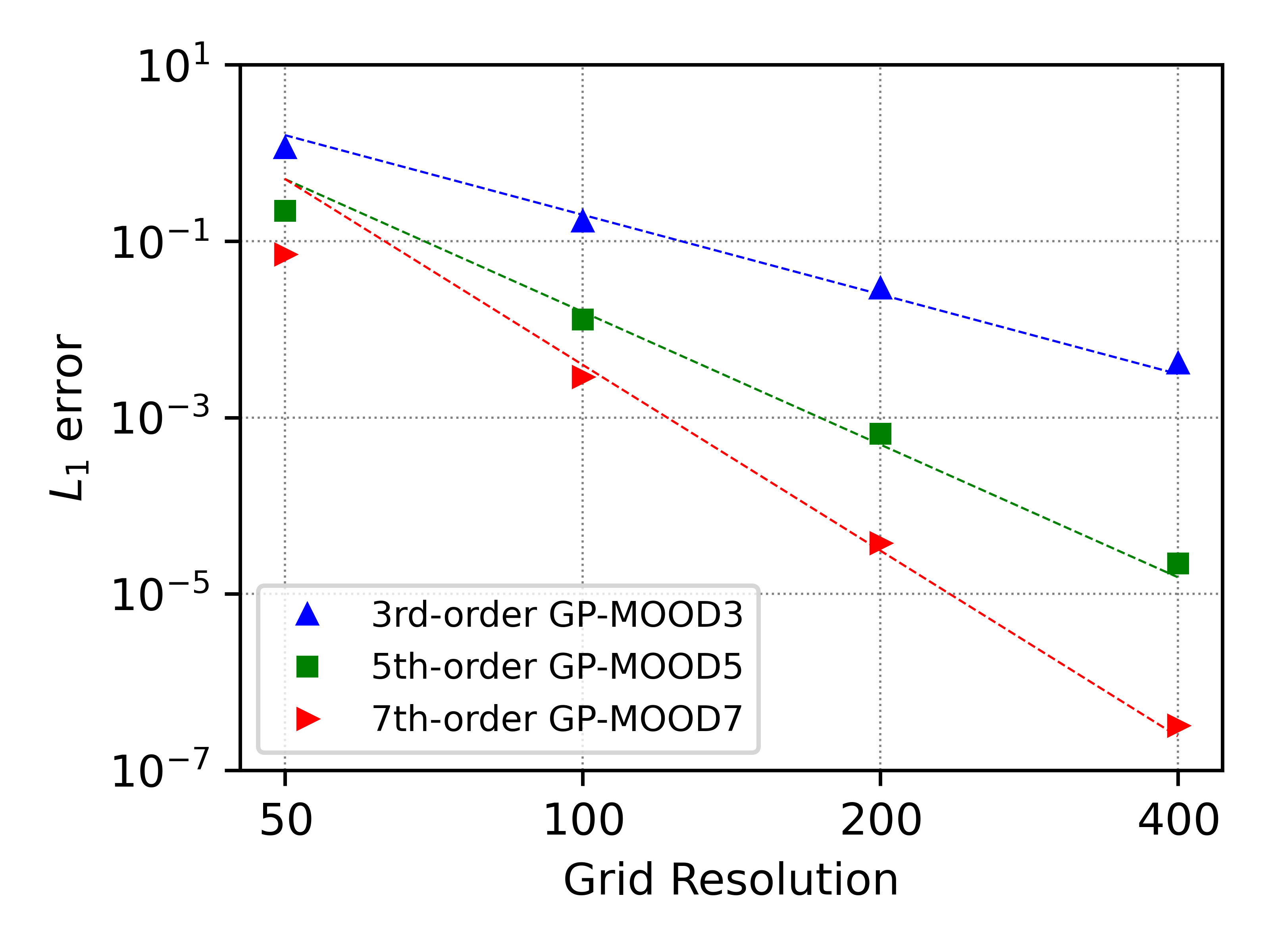
(a)

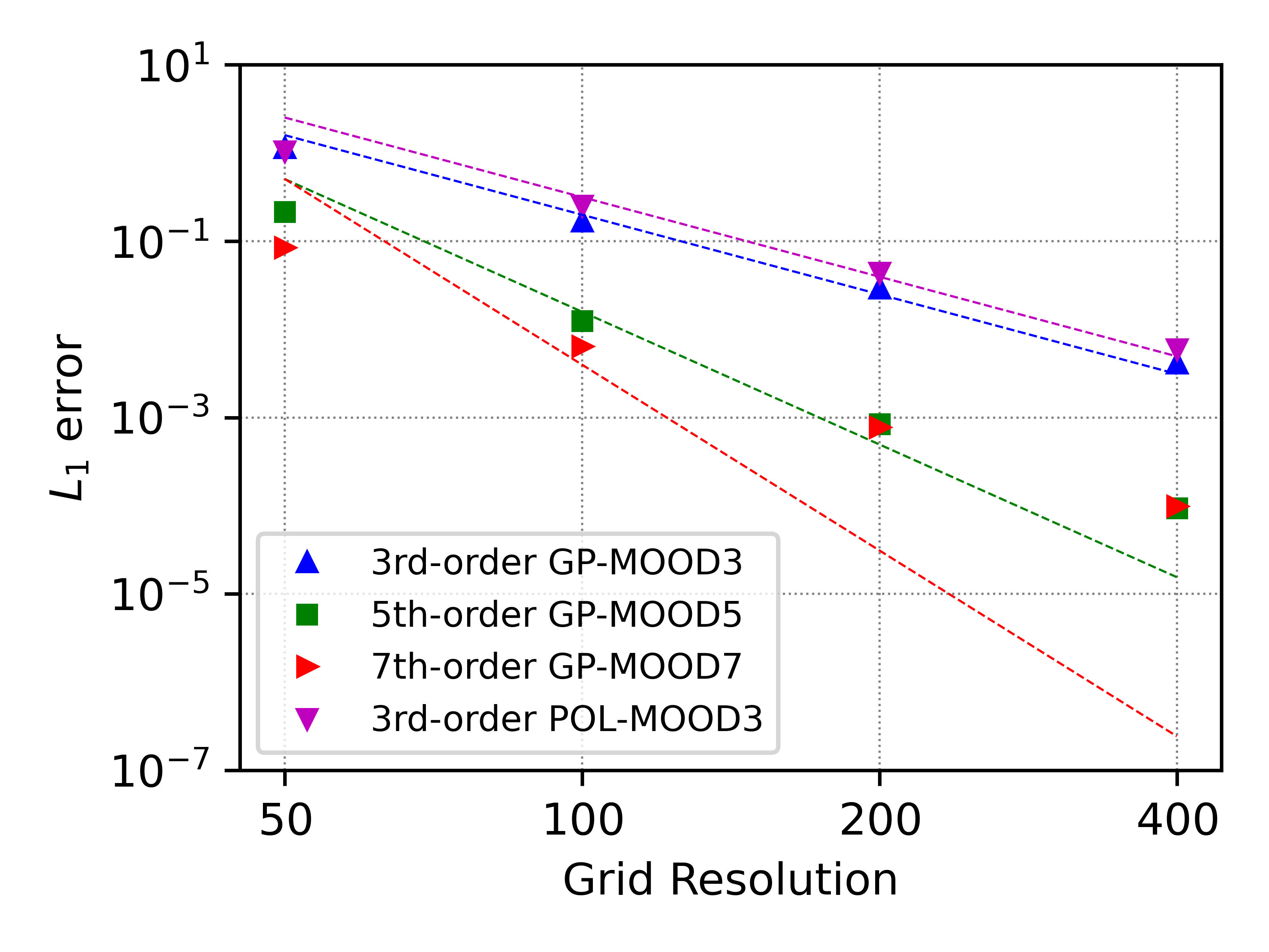
(b)

Figure 10: Convergence study on the 2D isentropic vortex advection for three different radii, stencils, and reconstructions. (left) The convergence rates on the blocky-diamond GP stencils. (right) The convergence rates on the cross-shaped stencils. CFL=0.8 is used for all cases with proper time step size reductions.

For GP, we set $\ell=1$ in all test cases considered here, based on our former studies on the a priori GP methods [20, 21]. Tested in Fig. 10 include the 3rd-order GP-MOOD3 (GP-R3 $\to$ FOG), the 5th-order GP-MOOD5 (GP-R5 $\to$ GP-R3 $\to$ FOG), and the 7th-order GP-MOOD7 (GP-R7 $\to$ GP-R3 $\to$ FOG). In Fig. 10(a), the results are solved on the blocky-diamond GP stencils as depicted in Figs. 1 and 2. In Fig. 10(b) though, the same tests are repeated on cross-shaped GP stencils that are the direct extension of the GP-R1 stencil in Fig. 1 to a bigger cross stencil by adding extra cells in each normal direction only according to the GP radius $R$. While the cross GP stencil and the blocky sphere stencil are the same for GP-R1, the size of the cross increases to the 9-point stencil for GP-R2 and 13-point for GP-R3.

The results of $L_{1}$ errors are reported in  Fig. 10 on four different grid resolutions, $N_{x}=N_{y}=50,100,200$, and $400$. In Fig. 10(a), the convergence rates of the three GP-MOOD methods on the corresponding diamond GP stencil follow the analytical convergence rates (dotted lines) of $(2R+1)$, showing the expected 3rd-, 5th-, and 7th-order rates, respectively. See also Table 2. The experimental order of convergence (EOC) is computed as

$$\mbox{EOC}=\frac{\ln(E_{c}/E_{r})}{\ln(2)},$$ (37)

where $E_{c}$ and $E_{r}$ are the $L_{1}$ errors on the coarse and the next coarse resolutions (e.g., $E_{c}$ on $50\times 50$ and $E_{r}$ on $100\times 100$), respectively. The demonstration of the full convergence rate in each GP-MOOD method proves that the GP-MOOD detection algorithms operate successfully without any erroneous order reduction on this smooth advection problem, and the solution evolves with the highest accurate, unlimited GP reconstruction method in each case.

However, in Fig. 10(b) and Table 3, the accuracy of GP-MOOD is heavily compromised when the solutions evolve on the smaller cross-shaped stencils (i.e., 9 vs. 13 stencil points for GP-MOOD5; 13 vs. 25 for GP-MOOD7. See Fig. 2). We see that the rate of convergence is disturbed in GP-MOOD5 and GP-MOOD7. In both cases, the orders of accuracy asymptotically converge at 3rd-order, with both errors reduced by about two orders of magnitude compared to the GP-MOOD3 error. We also show the convergence rate of the polynomial counterpart, POL-MOOD3, in Fig. 10(b) and Table 3. Similar to that of GP-MOOD3, the 3rd-order rate of convergence is achieved except that POL-MOOD3’s magnitude of the error on each grid resolution is about 1.5 times larger than the reported error with GP-MOOD3.

Table 2: Performance results of three different GP-MOOD algorithms on the blocky-diamond GP stencils.

Grid Resolution	GP-MOOD3			GP-MOOD5			GP-MOOD7
	$L_{1}$ errors	EOC		$L_{1}$ errors	EOC		$L_{1}$ errors	EOC
$50\times 50$	1.13746068e+00	–		2.22016430e-01	–		7.11860045e-02	–
$100\times 100$	1.67459246e-01	2.76		1.29737576e-02	4.10		2.90834888e-03	4.61
$200\times 200$	2.91650062e-02	2.52		6.60244975e-04	4.30		3.76226930e-05	6.27
$400\times 400$	4.11626679e-03	2.82		2.23315572e-05	4.89		3.21581083e-07	6.87

Table 3: Performance results of GP-MOOD5, GP-MOOD7, and POL-MOOD3 on the cross GP stencils. The performance of GP-MOOD3 is omitted here since there is no discrepancy between the cross and diamond stencil configurations for GP-MOOD3; see Table 2 for its performance.

Grid Resolution	GP-MOOD5			GP-MOOD7			POL-MOOD3
	$L_{1}$ errors	EOC		$L_{1}$ errors	EOC		$L_{1}$ errors	EOC
$50\times 50$	2.15245127e-01	–		8.50162184e-02	–		1.04593597e+00	–
$100\times 100$	1.24973881e-02	4.10		6.39925304e-03	3.73		2.54731899e-01	2.04
$200\times 200$	8.42402789e-04	3.89		7.75915293e-04	3.04		4.40709959e-02	2.53
$400\times 400$	9.37519200e-05	3.17		9.92175024e-05	2.97		5.96194298e-03	2.89

5.2 Shock-dominant benchmark test problems

Well-known standard shock-dominant benchmark problems in 1D and 2D are tested in this section to discuss the validity of our GP-MOOD solvers.

5.2.1 The Shu-Osher shock tube test in 1D

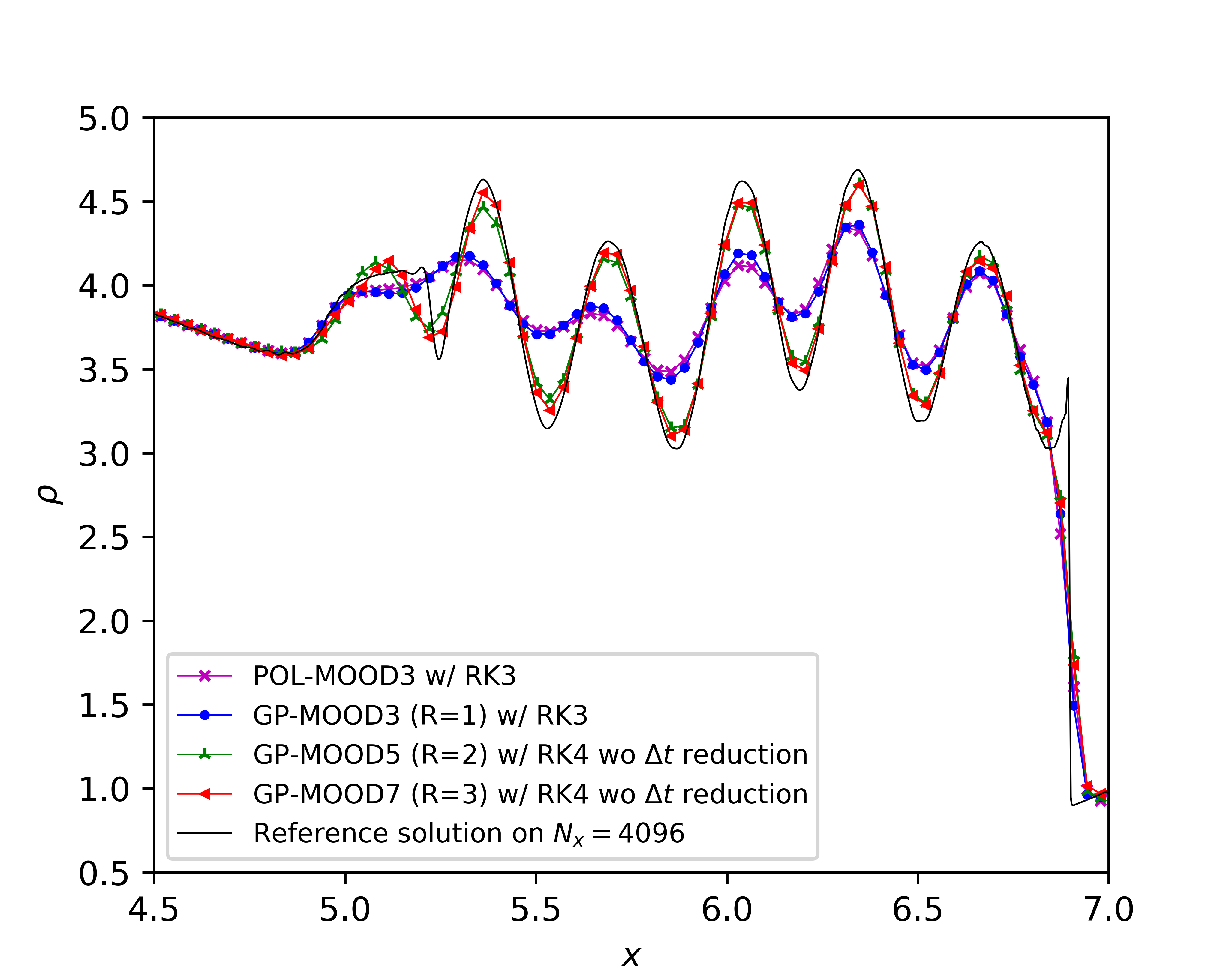
Figure 11: Result of the Shu-Osher shock tube test at $t=1.8$ using GP-MOOD3, GP-MOOD5, GP-MOOD7 with $\ell=6\Delta x$, CFL =0.8, resolved on 256 grid cells. The GP solutions are plotted along with the POL-MOOD3 solution on the same grid resolution. The reference solution is computed using POL-MOOD3 with SSP-RK3 without reducing $\Delta t$ on $N_{x}=4,096$.

The Shu-Osher shock tube problem [65] provides a good comparison study of different numerical algorithms to measure relative accuracy and diffusivity. The point of interest in this problem is to see how well different methods can produce the high and low-frequency regions of the density profile, as the Mach 3 shock wave travels from left to right into the initial low-frequency sinusoidal profile. As a result, the perturbed density is compressed at the shock-smooth profile interactions, creating a high-frequency trail of doubled-frequency waves to the left of the immediate post-shock region. Further down to the left in the post-shock region, attached to the tail of the high-frequency region is the low-frequency structure – now substantially sharpened from the initial sinusoidal profile due to the shock-steeping – where the perturbation returns to the original frequency of the unshocked initial wave. We follow the standard setup of the initial condition [65],

$$(\rho,u,p)=\begin{cases}(3.857143,\ 2.629369,\ 10.33333)&\text{if}\quad x<0.5,\\ (1+0.2\sin(5(x-4.5)),\ 0,\ 1)&\text{if}\quad x>0.5,\end{cases}$$ (38)

on a one-dimensional domain $[0,9]$ and we evolve the solution until $t=1.8$. The boundary condition at $x=0$ and $x=9$ is the fixed boundary condition that sets the initial values during the simulation. All simulations are computed on a grid resolution, $N_{x}=256$, except for the reference solution resolved on the 16 times more refined resolution, $N_{x}=4,096$, using POL-MOOD3 and SSP-RK3 without any time step reduction. The time steps of SSP-RK4 are reduced for GP-MOOD5 and GP-MOOD7 to match the accuracy of the spatial and temporal solvers.

Simulated results are compared in Fig. 11, where we display a zoomed-in view of the entire profile to focus on the solution comparison over the high-frequency region. Overall, all results produce acceptable density profiles capturing the assumed high-frequency amplitudes fairly well, conforming with the reference solution. The amplitude closest to the reference profile is achieved by GP-MOOD7, followed by GP-MOOD5, GP-MOOD3, and POL-MOOD3. It is quite impressive to see how closely the solutions produced by GP-MOOD5 and GP-MOOD7 follow the reference profile, with only on the grid resolution 16 times lower than the reference solution. To be more quantitative, we compare the maximum values of the density, measured at $x\approx 6.34$. The reference solution reaches $\rho\approx 4.69$, while both GP-MOOD5 and GP-MOOD7 give $\rho\approx 4.60$, providing 98% accuracy in predicting the largest amplitude with only utilizing 6.25% of the reference grid resolution. For GP-MOOD3, $\rho\approx 4.36$, yielding 93% accuracy, while $\rho\approx 4.32$ with 92% accuracy for POL-MOOD3.

Lastly, we remark that it is crucial to utilize the CSD criterion described in Section 3.4 in order to produce the well-systematic solutions as in Fig. 11, namely, GP-MOOD7 being the most accurate, GP-MOOD5 intermediate, and GP-MOOD3 the least accurate. If CSD is not employed, numerical diffusivity of the GP solutions becomes excessive, and their solution qualities turn into a disorderly fashion, e.g., the GP-MOOD5 solution turns out to be as diffusive as the GP-MOOD3 solution.

5.2.2 The Sedov explosion test in 2D

Next, we revisit the Sedov blast test [66]. The primary purpose is to test how well the GP methods retain the symmetry of the self-similar evolution of the spherical shock propagation outward from a highly pressurized point-source at the domain center, $(x,y)=(0,0)$. We discretize a 2D outflow domain, $[-0.5,0.5]\times[-0.5,0.5]$, at a grid resolution, $256\times 256$, where the initial condition is configured by following the description in [67].

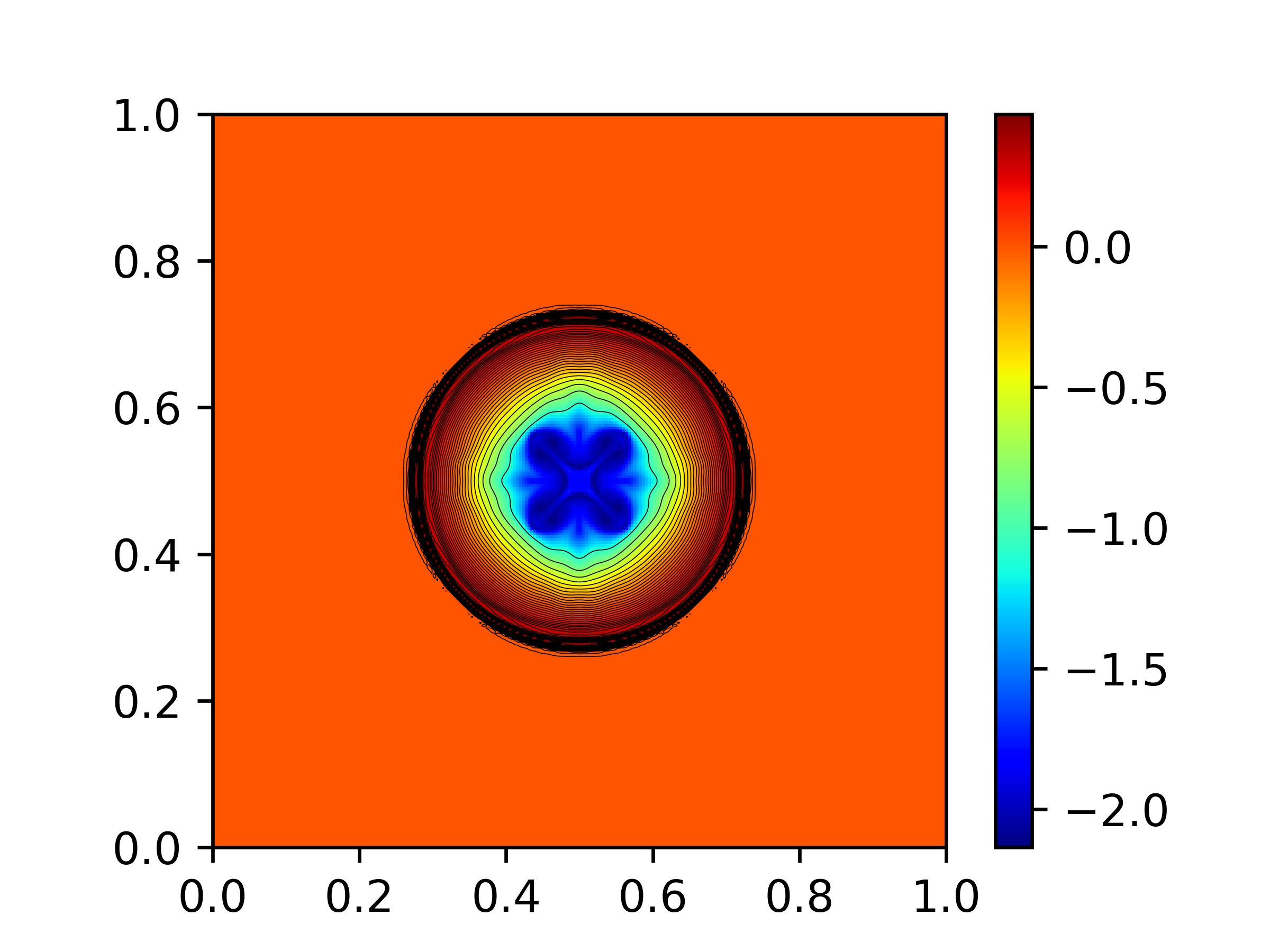
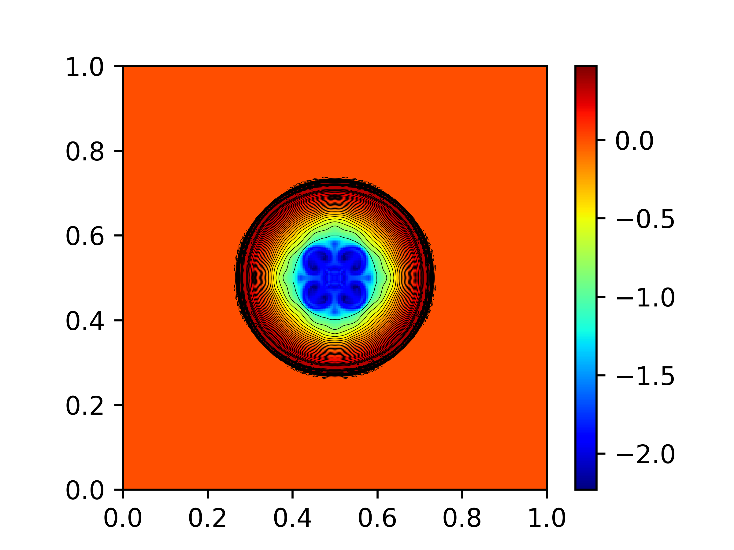
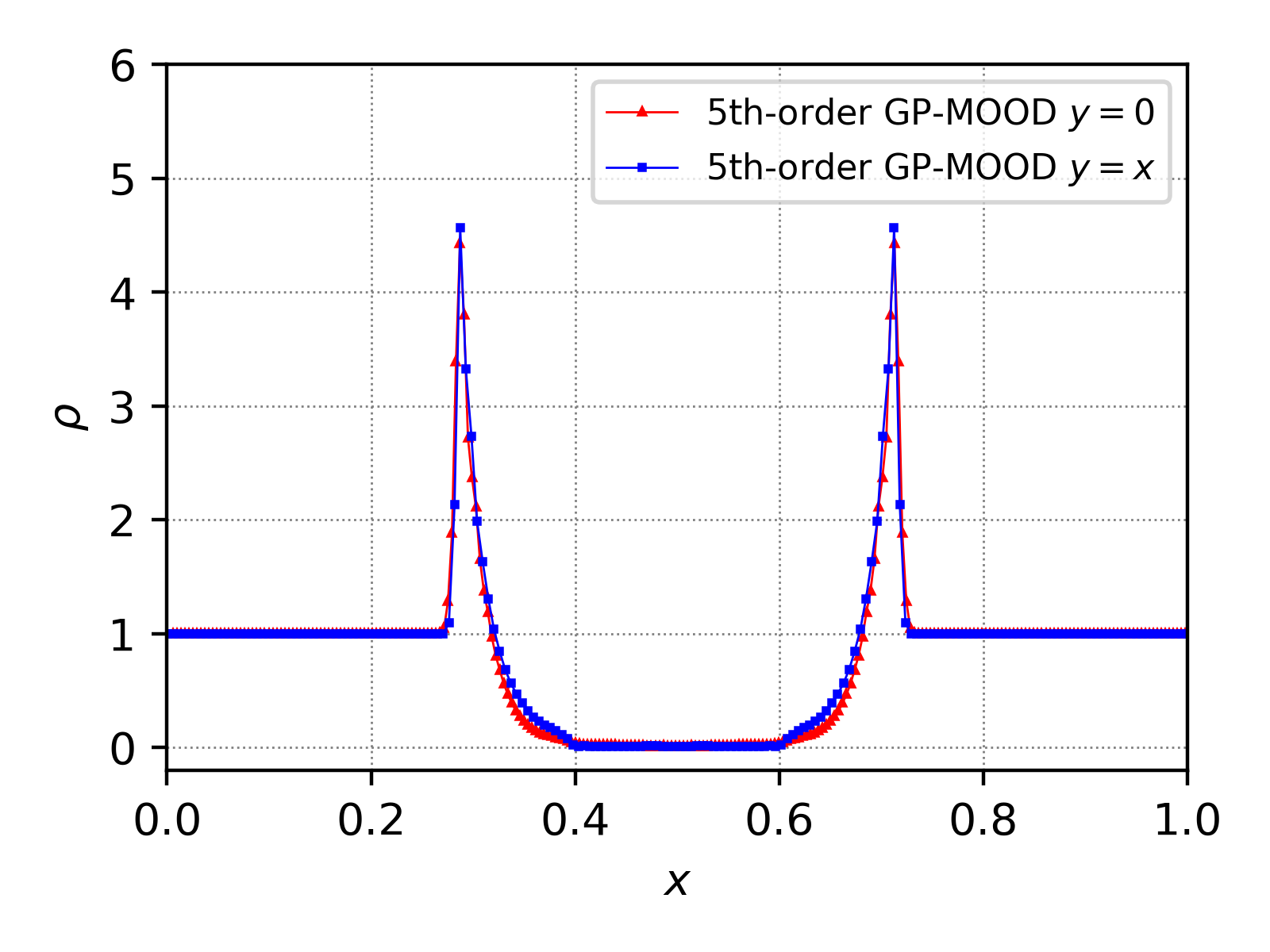
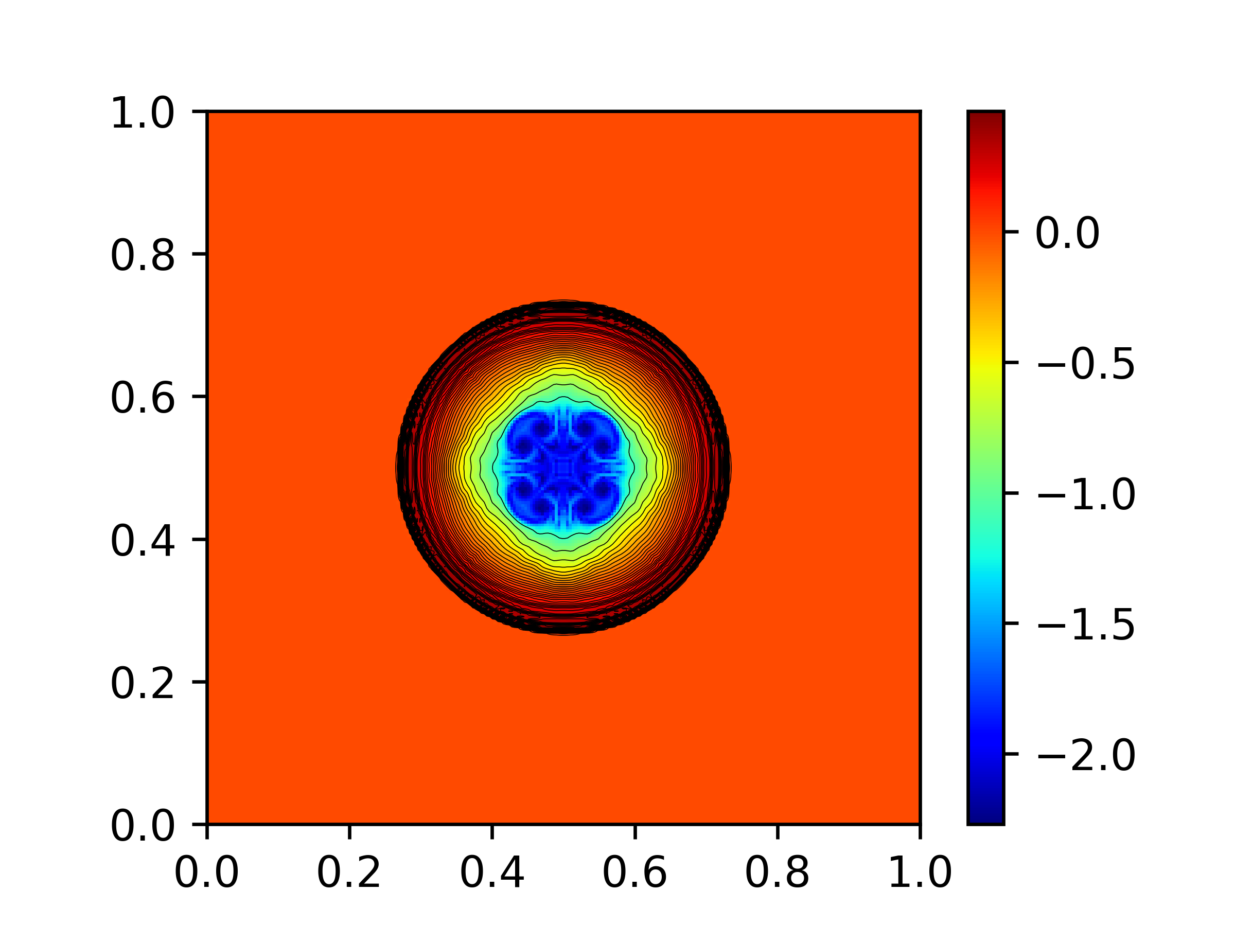
Figure 12: Density profiles of the Sedov test problem at $t=0.2$ on a $256\times 256$ grid resolution. Three GP-MOOD methods are solved using $\ell=12\Delta$ with $\Delta=\Delta x=\Delta y$ and CFL = 0.8. We over-plot 40 contour lines. (top) The 2D density profile (log scale) of GP-MOOD3 (left); the corresponding sectional profiles (linear scale) along the $x$-axis (red) and the diagonal $y=x$ (blue) (right). (middle) The solutions of GP-MOOD5. (bottom) The solutions of GP-MOOD7.

Three test results are shown in Fig. 12, including the density profiles of GP-MOOD3, GP-MOOD5, and GP-MOOD7. All three results maintain the spherical evolution of the exploding shock satisfactorily. Unlike the failed cases in Fig. 8, the central region exhibits the details of the low-density flow structures as the flow is driven radially outward with the expansion. The expanding flow feels unavoidably the grid-aligned dependency, leaving in the central region the grid-aligned artifacts along the $x$- and $y$-axis, as well as the round-shaped diagonally-aligned structures. We observe that those structures become more expressive as the accuracy order of GP-MOOD increases. The sectional density profiles show that the peak amplitudes along the $x$-axis and the domain diagonal $y=x$ agree well with each other.

5.2.3 The double Mach reflection problem in 2D

The next 2D test problem is the double Mach reflection problem by Woodward and Colella [68]. This test problem has been widely chosen to demonstrate the code capability of handling a strong shock propagation, reflections, and subsequent developments of vortical roll-ups, including our former study on the a priori GP-WENO finite difference method [21].

The initial configuration sets up an inclined planar Mach 10 shock initially positioned on the left side of the rectangular domain. $[0,4]\times[0,1]$. The shock front makes a $60^{\circ}$ incident angle to the reflecting wall at the bottom. As the shock propagates to the right side of the domain, the shock is reflected from the bottom wall, which forms two Mach stems, two contact discontinuities, and the dense jet along the bottom reflecting wall. One of the contact discontinuities emanates from the triple-point, where the contact discontinuity meets the unreflected Mach 10 shock and the Mach stem perpendicular to the bottom wall. The slip surface of this contact discontinuity undergoes Kelvin-Helmholtz instabilities, the amount of which is a sensitive function of the amount of numerical dissipation in the algorithm under consideration. Thereby, the problem is often used as an indication to quantify each method’s numerical dissipation by monitoring the number of Kelvin-Helmholtz vortical roll-ups at the end of the simulation. We run the test until $t=0.25$. See [68] for details of the initial and boundary setup configurations.

Fig. 13 displays three density plots of GP-MOOD3, GP-MOOD5, and GP-MOOD7, all integrated using SSP-RK3 without any time step reduction. They are solved on a grid resolution of $800\times 200$ with CFL=0.8. We set the GP hyperparameter, $\ell=12\Delta$, where $\Delta=\Delta x=\Delta y$. We see that the degree of the Kelvin-Helmholtz instability formation is most pronounced with GP-MOOD7 and intermediate with GP-MOOD5. On the other hand, the instability development is suppressed with GP-MOOD3 at the slip surface without any sign of vortical roll-up. The results can also be compared with our previous results obtained by the a priori GP-WENO finite difference method, see Fig. 15 in [21]. On the same grid resolution, it is seen that the roll-ups are more evident with GP-MOOD3 than the result previously predicted by the 5th-order GP-WENO method therein, namely, panel (c) of Fig. 15 in [21]. Although this comparison may not be a direct point-to-point lateral comparison, given the two different methods in comparison are the finite difference method (GP-MOOD5) with CFL=0.8 and the finite volume method (GP-WENO GP-R2) with CFL=0.4, this comparison demonstrates that there is smaller numerical dissipation in GP-MOOD5 than GP-WENO GP-R2. This result can provide a guideline for our future study to conduct a more direct comparison between the two same consistent discretization methods, e.g., two finite volume methods of the a posteriori GP-MOOD5 scheme and a new a priori GP-WENO GP-R2 scheme. Such a comparison study will shed light on understanding how much numerical dissipation is present in the two different shock capturing paradigms, a posteriori and a priori methods.

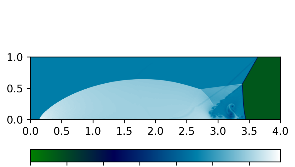
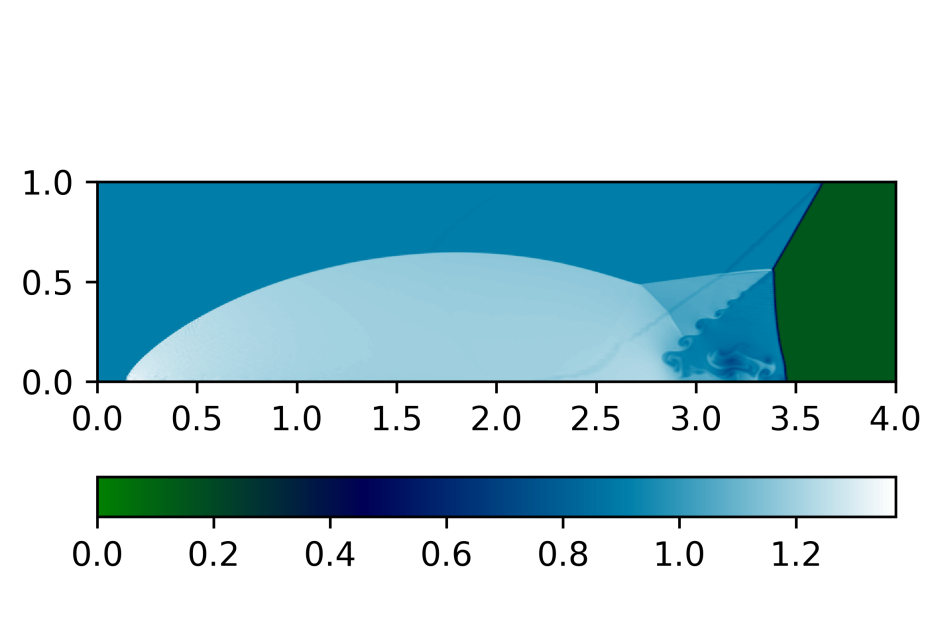
Figure 13: The 2D double Mach reflection problem on an $800\times 200$ mesh resolution. The density at $t=0.25$ is plotted using three different GP-MOOD methods, all integrated with SSP-RK3, CFL=0.8, and the HLLC fluxes. The choice of $\ell=12\Delta$ with $\Delta=\Delta x=\Delta y$ is used in all cases. (top) The 3rd-order GP-MOOD3. (middle) The 5th-order GP-MOOD5. (bottom) The 7th-order GP-MOOD7.

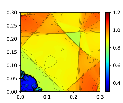
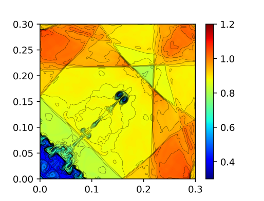
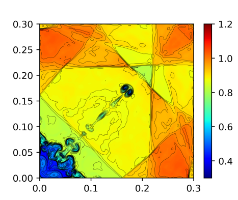
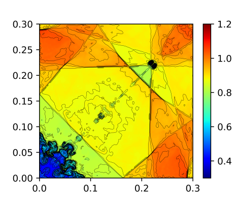
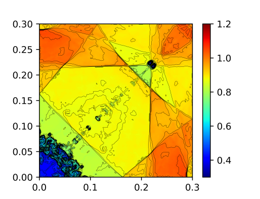
Figure 14: The density plots at $t=2.5$ of the implosion test in 2D. From top left to top right and bottom left to bottom right, the solutions are computed using POL-MOOD3 without CSD, GP-MOOD3 without CSD, POL-MOOD3 method with CSD, GP-MOOD3 with CSD, GP-MOOD5 with CSD, and GP-MOOD7 with CSD. SSP-RK3 is used in all cases without $\Delta t$ reduction and using CFL=0.8. The choice of $\ell=12\Delta$ with $\Delta=\Delta x=\Delta y$ is used in all cases. The contour lines are plotted for 40 evenly-spaced density values.

5.2.4 The implosion problem in 2D

As for our last benchmark test, we consider the 2D implosion problem introduced by Hui et al. [69] and further simplified by Liska and Wendroff [70]. We set up the initial condition by following [70] on a square domain, $[0,0.3]\times[0,0.3]$. All four boundaries are reflecting walls, which bounce off a converging shock wave that is initially launched by the initial planar discontinuity along $x+y=0.15$. The over-pressurized flow above the line will send the planar shock wave towards the origin,$(x,y)=(0,0)$. As it moves, the shock wave interacts with the reflecting walls and produces a formation of a double Mach reflection sliding along the left and the bottom wall boundaries. This Mach reflection forms two jets that move into the origin along the boundaries at the exact same time, ultimately colliding each other simultaneously at $(x,y)=(0,0)$. This dynamics is similar to that of the double Mach reflection test in Section 5.2.3. The two-jet collision then ejects a new collimated narrow jet from the origin toward the upward domain diagonal direction. Due to the reflecting walls, the subsequent shocks are continuously bounced back into the domain, creating unceasing nonlinear shock-jet interactions. These interactions progressively push the diagonal jet diagonally upward while at the same time turning its shape into a longer and narrower jet over time. The mushroom heads, fingers, and the fine elongated filaments are generated at the diagonal jet surface – the contact discontinuity separating two density regions – as a result of the Richtmyer-Meshkov instability. Their morphology is sensitive to numerical dissipation, thereby can be a good indicator to distinguish differing methods. Besides, it is crucial to maintain the diagonal symmetry at all times during the simulation.

In Fig. 14, we present six results of the density profiles at $t=2.5$ computed on a $400\times 400$ grid resolution. We find that the CSD switch introduced in Section 3.4 plays an imperative role in simulating the diagonal jet dynamics successfully. To demonstrate its impact, we ran the test with and without the CSD switch. The test cases in the comparison include, in the order from top left to top right and bottom left to bottom right, the 3rd-order polynomial POL-MOOD3 method without CSD, the 3rd-order GP-MOOD3 method without CSD, the 3rd-order polynomial POL-MOOD3 method with CSD, the 3rd-order GP-MOOD3 method with CSD, the 5th-order GP-MOOD5 method with CSD, and finally the 7th-order GP-MOOD7 method with CSD. All spatial solvers are integrated with SSP-RK3 without any time step reduction using CFL=0.8.

As can be seen in the first two panels, no diagonal jet is present without CSD in both of the 3rd-order results based on polynomial and GP reconstructions. On the contrary, the jet propagation is clearly captured in the same solver calculations with CSD (the third and fourth panels), by which numerical dissipation is better controlled without being too diffusive. From this experiment, we conclude that the complete absence of the jet dynamics in the first two results is related to the excessive amount of numerical dissipation in the conventional MOOD approach [24, 25, 26, 27], which suppresses the anticipated jet formation at the early stage of the evolution. Activating the CSD check addresses this issue and imposes the proper amount of diffusivity in the flow. Apart from the presence of the jet, its shape is also interesting. In all four results with CSD the jet retains exact symmetry, a key indication that has been widely adopted to test each method’s capability of maintaining reflective symmetry to machine precision [71, 72, 58]. We also observe that the distance the jet head travels from the origin is related to the amount of numerical dissipation in the tested methods. The tip of the mushroom head reaches $x=y\approx 0.22$ for GP-MOOD5 and GP-MOOD7, $x=y\approx 0.18$ for GP-MOOD3, and $x=y\approx 0.17$ for POL-MOOD3. Similarly, a long-traveled jet is reported in [72] using the polynomial-based PPM method.

5.3 Highly compressible flow tests with strong Mach jets in 2D

This section considers two configurations of highly compressible supersonic astrophysical jets that propagate into dense and light ambient gases.

5.3.1 Single Mach 100 light jet

Our first selection of a test problem in highly compressible flows is the extragalactic astrophysical jet evolution studied by Balsara [73]. This setup is the second type of the two jet configurations tested in [73], called the Mach 100 light adiabatic jet that enters the ten times denser ambient fluid from a narrow slit in the domain bottom. Of the two configurations therein, this light jet problem is considered to be more stringent than the first jet problem to simulate, where the first jet problem considers the Mach 800 dense jet propagation into the ten times less dense ambient fluid [74, 73]. We report our GP-MOOD results on the more challenging light dense jet case only, although we were able to run the dense jet problem successfully. Magnetized versions of the astrophysical jet have been also reported in [75, 76].

The computational domain is a square outflow box, $[0,1.5]\times[0,1.5]$, except for the narrow slit, $[0.7,0.8]$ at $y=0$, through which the Mach 100 jet is injected into the domain via the inflow boundary condition fixed by the jet condition,

$$(\rho,u,v,p)_{\mbox{jet}}=(\gamma,0,100,1),\;\;\;0.7\leq x\leq 0.8\;\;\mbox{and}\;\;y=0,$$ (39)

where $\gamma=1.4$. The jet’s Mach number is hence 100. The ambient fluid is initialized by

$$(\rho,u,v,p)_{\mbox{ambient}}=(10\gamma,0,0,1).$$ (40)

There are a couple of important features to monitor in this problem, including (i) the symmetric evolution of the jet, (ii) positivity preservation throughout the simulation time, and (iii) the internal structure of the “cocoon” that surrounds the jet.

From left to right in Fig. 15, each column shows the results using GP-MOOD3, GP-MOOD5, and GP-MOOD7, which are integrated until $t=0.04$ on a $600\times 600$ grid resolution. Plotted in each row from top to bottom are the density profiles at $t=0.01,0.02,0.03$, and $0.04$, respectively. As before, all results are computed with CFL=0.8 (a relatively very high CFL number for this simulation), and SSP-RK3 without any time step reduction. In this simulation and the double jet collision simulation in the next section we use the HLL solver [62] to mitigate the grid-aligned carbuncle instability [63] at the foremost shock front. The overall jet evolution and the subsequent flow structures are comparable to the results in Fig. 4 of [73], where the reported simulation time was $t=0.03$. We doubt that, based on the jet height, the simulation could have run longer than $t=0.03$, close to $t=0.04$ as we report here. We were also able to confirm this using FLASH’s [67] unsplit hydrodynamics solver, which is a gas dynamics version of the unsplit magnetohydrodynamics solver by Lee & Deane [77]; Lee [78].

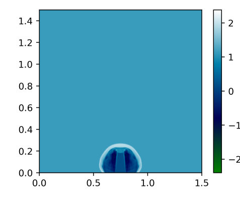
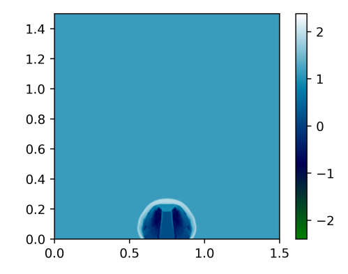
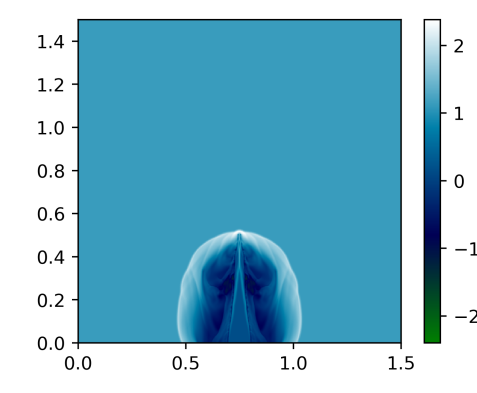
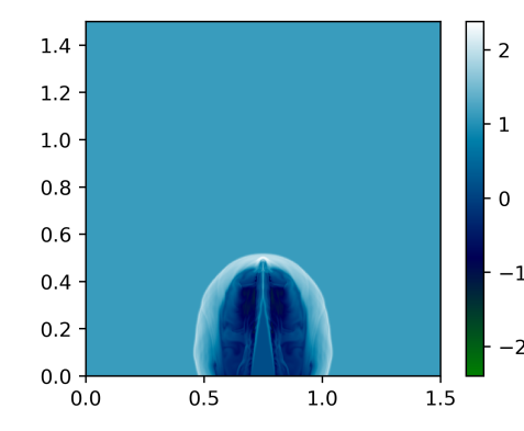
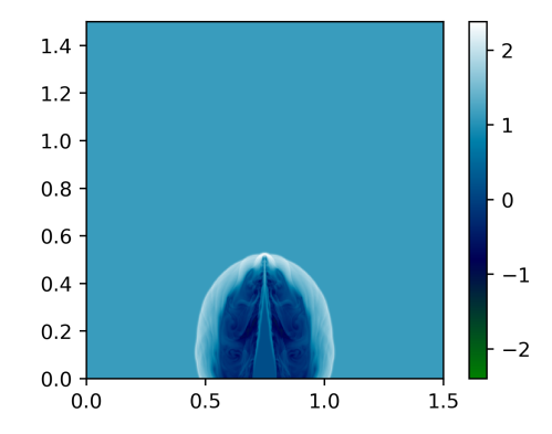
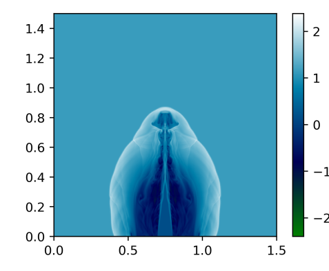
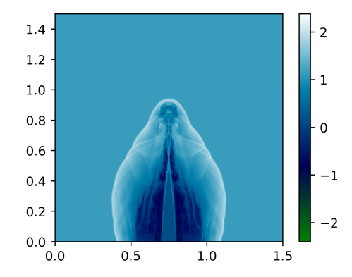
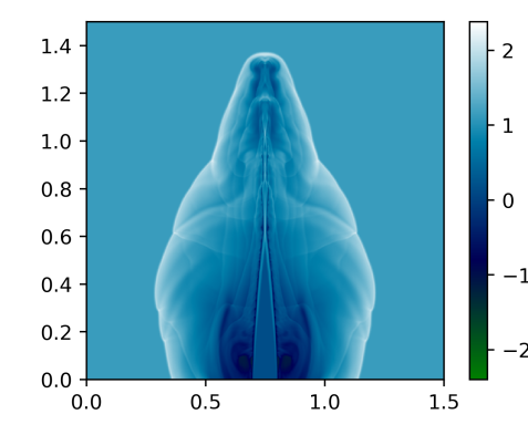
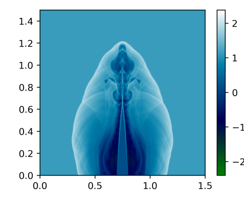
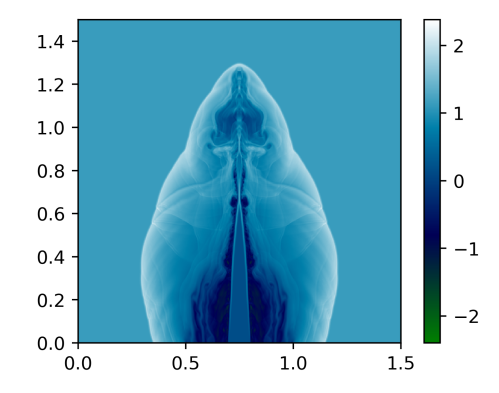
Figure 15: The single Mach 100 light jet problem is resolved on a $600\times 600$ grid resolution. Density profiles are displayed. From left to right, the results are computed using GP-MOOD3, GP-MOOD5, and GP-MOOD7, while from top to bottom, the densities are plotted at $t=0.01,0.02,0.03$, and $0.04$. Except for the use of HLL, the rest of the runtime parameters are the same as before, including CFL=0.8, $\ell=12\Delta$ with $\Delta=\Delta x=\Delta y$.

In the early stage at $t=0.01$, the jet has only propagated through approximately 15% of the domain in height, pushing the denser gas and building up the density and pressure. Since the ambient gas is denser, the lighter jet’s push moving at Mach 100 creates a highly compressed region at the nose of the jet, forming a curved shock wave that drapes down to the bottom. As the jet further pushes the ambient denser gas, the shock wave expands into an oval sheath that drapes to the bottom. The high-pressurized flow just inside the sheath pushes the low dense gas between the jet and the sheath further inward, squeezing the jet. As a result, the blunt jet nose turns into a thinner and pointy shape, as illustrated in the plots at $t=0.02$. This change of the nose shape results in a sudden speed-up of the nose relative to the shock front, which is seen as the shock wave penetration of the pointy jet nose at $t=0.02$. Sooner or later, the pointy nose feels the pushbacks from the denser and highly pressurized shock front and decelerates, increasing the nose size a bit. This can be seen in the results at $t=0.03$, where the formerly pointy jet nose at $t=0.02$ around $y\approx 0.4$ with GP-MOOD3 and GP-MOOD5, $y\approx 0.5$ with GP-MOOD7, now has grown to a wider jet at $t=0.03$.

This motion of acceleration and deceleration repeats and changes the jet into a sausage-like shape. As a result, the previously oval-shaped shock outer surface at $t\leq 0.02$ turns into a more irregular shape, such as an outer layer of Matryoshka dolls (or Russian dolls), as plotted at $t=0.03$ and $0.04$. Another consequence of the acceleration-deceleration process is the shock waves reflected from the kinks at the shock front, each of which is created when a newly formed pointy jet nose starts to push the shock front with sudden acceleration. This push accelerates the shock front ahead of the jet’s nose and stretches the sheath further, deforming the overall envelope from a clean oval surface to an elongated Matryoshka doll shape. A new pair of kinks is generated at the shock surface, symmetrically around the center of the jet, $x=0.75$. We see that a rich structure of the shock waves is fully present in the cocoon region, i.e., the region between the shock front sheath and the jet.

In contrast, such an acceleration and deceleration process is not present in the other dense jet configuration [73] since, in this case, the jet is dense enough to retain its width without experiencing a sausage-like mode. The flow in the cocoon region therefore becomes relatively quiescent without shock waves compared to the light dense jet case considered here.

We report in Fig. 15 that all three GP-MOOD methods successfully produce the relevant physics of the flow. The MOOD approach in all cases strictly enforced the positivity preservation without applying any additional positivity preserving mechanism, including a fictitious floor value approach or the self-adjusting positivity preserving strategy proposed in [73]. The acceleration-deceleration process of the jet makes the cocoon flow filled with the reflected shock waves. All three GP-MOOD methods are well capable of capturing these shock structures without any artifacts, as well as the sharp profile of the shock front during the run. All results reveal a great number of fine details of the reflected shock waves. There are small-scale Kelvin-Helmholtz instabilities driven by the upward and the downward flows in the low dense valley region between the jet and the high dense region where the reflected shocks are present. The flow attached to the jet experiences upward movements as the jet drags the flow. Trapped between the upward moving jet and the the upward moving shock-dominant region, the low-dense valley feels the downward flow motions, creating small-scale Kelvin-Helmholtz instabilities. We see that more abundant small-scale flows are featured as the solution accuracy increases from the 3rd-order GP-MOOD3 to the 7th-order GP-MOOD7.

The flow evolution of this problem is truly non-linear, with continuous interactions between the lighter jet and the denser ambient flows. Hence, the end results vary with the methods and parameters used for each run. This can be easily seen in different heights of the foremost shock front and different shapes of the shock front sheath in the three solutions. Such flows sensitively depend on the sausage-mode evolution of the jet and the corresponding acceleration-deceleration process. Interestingly, the tallest height is seen in the GP-MOOD3 solutions, while the smallest is in the GP-MOOD5. The mirror symmetry around $x=0.75$ is preserved well in all runs.

Lastly, we report that the number of cells that are iterated for order decrements in the MOOD loop is less than 3.5% of the entire cells in each step, implying 96.5% of the domain are stably solved by the highest accurate unlimited GP reconstruction method during the run.

5.3.2 Double Mach 800 jet collision

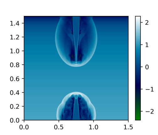
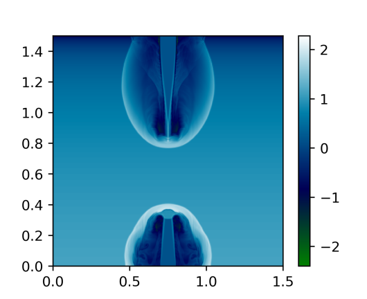
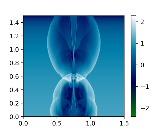
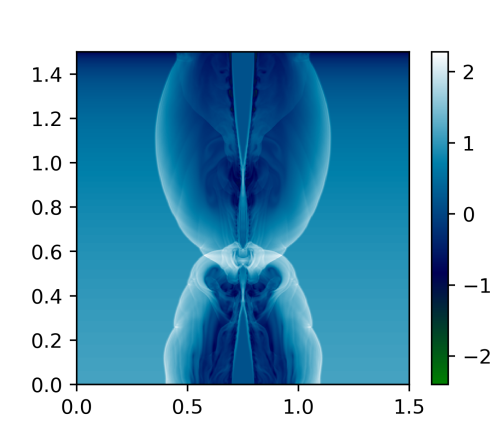
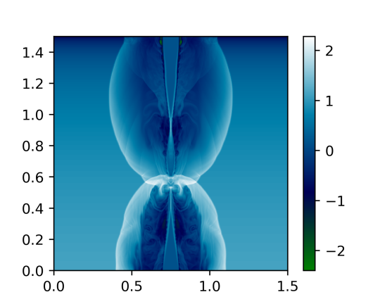
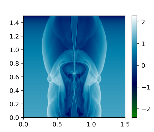
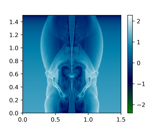
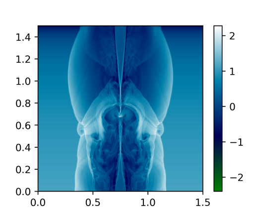
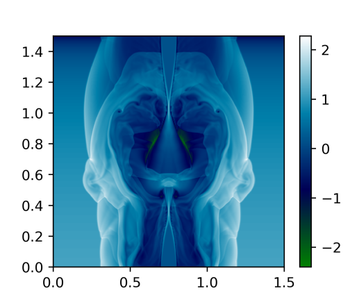
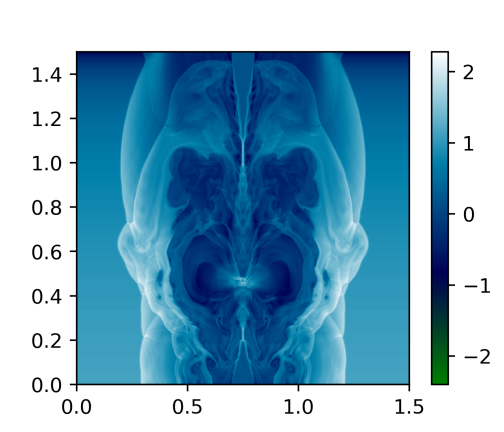
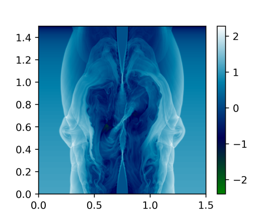
Figure 16: The double Mach 800 jet collision problem is resolved on a $600\times 600$ grid resolution. Density profiles are displayed. From left to right, the results are computed using GP-MOOD3, GP-MOOD5, and GP-MOOD7, while from top to bottom, the densities are plotted at $t=0.002,0.003,0.004$, and $0.005$. The runtime parameters are the same as the single jet problem.

In the next problem, we extend the previous Mach jet configuration to a double Mach jet collision that leads to a more violent jet-jet head-on collision. The initial condition of the single Mach 100 light jet in Section 5.3 is modified to add two new configurations. First, the density of the ambient flow is stratified following

$$\rho_{\mbox{ambient}}=-9.24y+14,\;\;\;0\leq y\leq 1.5,$$ (41)

which makes the density at the bottom to be 100 times heavier than the top, i.e., $\rho_{\mbox{ambient}}(0)=14.0$ and $\rho_{\mbox{ambient}}(1.5)=0.14$. Second, we modify the jet configuration by introducing a second Mach jet injected from the top, and at the same time, increasing the two jets’ injection velocity by eight times, i.e.,

$$(\rho,u,v,p)_{\mbox{jet}}=(\gamma,0,800,1),\;\;\;0.7\leq x\leq 0.8,$$ (42)

both at $y=0$ and $y=1.5$ with $\gamma=1.4$. Since the ambient gas density is ten times lighter than the jet at $y=1.5$, the top jet becomes a dense Mach 800 jet, while the bottom jet remains as a light Mach 800 jet similar to the previous single jet setup.

In Fig. 16, from the left to right columns, we display the density evolutions of GP-MOOD3, GP-MOOD5, and GP-MOOD7. From top to bottom, the density profiles are plotted at $t=0.002,0.003,0.004$, and $0.005$. The top jet propagates through the ambient flow as a dense jet up to $y\approx 1.3637$, beyond which the ambient density becomes denser than the jet’s density. The jet then becomes a light jet and starts to undergo the sausage-like mode, as explained in Section 5.3. This is seen in the density results at $t=0.002$, where the top jet starts to get significantly squeezed into a narrower shape for $y\leq 1.3637$. The top jet moves faster than the bottom jet towards the collision point since the top jet propagates through the ambient density that is lighter in the top part of the domain. The shape of the outer shock wave sheath still remains as a clean oval shape for the top dense jet, while the bottom light jet’s sheath already exhibits a pair of kinks at $y\approx 0.22$.

At $t=0.003$, the two jets have already made a head-on collision. The collision produces highly turbulent fluid motions that are progressively amplified as the two jets continue to make their ways in the opposite directions for $t\geq 0.003$. Driven by the turbulence, the low-dense gas in the valley pushes the high-dense gas outward, which further excites the Rayleigh Taylor instabilities in the already Kelvin-Helmholtz unstable gas in the cocoon. It is observed that the symmetry is well preserved up to $t=0.003$ in all three solutions. However, developments of asymmetric flows are seen in the two higher order solutions later times. For instance, with GP-MOOD7 at $t=0.004$, a small region of asymmetrical flow is observed at $(x,y)\approx(0.75,0.71)$, where the two jets make a strong collision and keep pushing each other. With GP-MOOD5, a flow asymmetry is slightly delayed and seen at $t=0.005$ around $(x,y)\approx(0.75,0.45)$. By $t=0.005$, the GP-MOOD7 solution has evolved into a more asymmetrical flow in the central region. We relate this asymmetry issue with the recent study by Fleischmann et al. [79]. The study demonstrates that symmetry-breaking phenomena, particularly with shock interactions and turbulent structures, are closely associated with vanishing numerical viscosity. As such, high-order methods and highly resolved grid solutions are more prone to asymmetrical flow developments. The authors conclude that the main source of these asymmetric instabilities originates from floating-point truncation errors that grow rapidly over time. Such errors result from algorithmic artifacts (e.g., the lack of associativity) and do not originate from the nature of high-order schemes. Given that our GP-MOOD methods do not suffer from asymmetric instabilities in other problems, the flow asymmetries in our results with GP-MOOD5 and GP-MOOD7 may well be addressed with more rigorous code implementations that strictly impose the proposed associativity arithmetics as studied in [79]. We leave a further study on this topic in our future work.

Lastly, we report that the number of cells that undergo the order decrement in the MOOD loop remains less than 5.5% of the entire cells in each step before the jet-jet collision, which grows as high as 6.7% by $t=0.005$. Although this test is the most stringent problem in this paper in terms of the shock strength and the flow compressibility, about 93% of the domain is shown to be stable enough with the solution by the high-order unlimited linear GP reconstruction methods. This finding can support the algorithmic advantage of MOOD’s a posterior strategy over the conventional a priori shock-capturing strategy that requires actively employing computationally expensive nonlinear limiters all the time.

6 Conclusion

We have presented multidimensional, positivity-preserving high-order (3rd-, 5th-, and 7th-order) finite volume GP methods integrated in the MOOD framework. Extended from the existing polynomial-MOOD methods, the GP-MOOD methods replace the unlimited polynomial reconstruction schemes with a new set of unlimited GP reconstruction algorithms that are genuinely multidimensional. The GP-MOOD methods have shown that they can deliver non-oscillatory, highly accurate, and positive-preserving numerical solutions on a set of stringent benchmark problems, including two highly compressible supersonic Mach jet test problems.

Compared to the existing 2D polynomial MOOD methods, the GP-MOOD methods can deliver high-order solutions using smaller local stencil sizes, e.g., the 5-points GP stencil for the 3rd-order GP-MOOD3, the 13-points GP stencil for the 5th-order GP-MOOD5, and the 25-points GP stencil for the 7th-order GP-MOOD7. The GP-MOOD methods balance the two demanding numerical requirements, solution accuracy and stability, via the series of detection algorithms comprising the MOOD loop. The solution accuracy is decreased at troubled cells from the highest accurate choice of an unlimited GP reconstruction algorithm down to the least accurate first-order Godunov method, by which GP-MOOD gains increasing numerical stability. This study also introduced a new detection switch called the “Compressibility-Shock Detection” (or CSD) that improves the excessive diffusivity in the existing polynomial MOOD methods. We have demonstrated that CSD is essential to capture some crucial flow dynamics that are signature to certain benchmark problems.

We demonstrate that the percentage of those troubled cells, where GP-MOOD’s order decrements takes place, is only a fraction of the entire domain and never exceed 10%. Our finding is consistent with the former studies on the polynomial MOOD methods [26, 27, 34].

Our work in this paper designs our GP-MOOD methods for the hyperbolic systems of the Euler equations in 1D and 2D. However, our study is not limited to this model; the GP-MOOD methods can seamlessly be extended to the 3D version of the Euler equations as well as other physics system such as magnetohydrodynamics, relativistic (magneto)hydrodynamics, to name a few. Lastly, we remark that the accuracy of GP-MOOD is not limited to 7th-order but can be further extended to a higher accuracy of $(2R+1)$ with $R>3$. These topics will be investigated in our future work.

Appendix A Tabulated example of $\Delta_{mn,d}$ values

We give the tabulated values of $\Delta_{mn,d}$ in Eq. (13) for the computation of the prediction vector at the Gaussian quadrature point, $(x,y)=(x_{i+1/2},g_{1})$, depicted in Fig. 17. See also Fig. 3. We give an example for the 3rd-order GP-MOOD3 with a GP radius $R=1$, for which the default quadrature rule is the 2-point, 4th-order quadrature rule,

$$\int_{y=-\frac{\Delta y}{2}}^{y=\frac{\Delta y}{2}}f(x,y)\simeq w_{1}f(x,g_{1})+w_{2}f(x,g_{2}),$$ (43)

where $g_{1}=\frac{\Delta y}{2\sqrt{3}},g_{2}=-\frac{\Delta y}{2\sqrt{3}},$ and $w_{1}=w_{2}=\frac{1}{2}$. The values of $\Delta_{mn,d}$ for each $d=x,y$ are tabulated in Table 4 and Table 5, respectively. The indices $m$ and $n$ represent the cell index in the 5-point GP stencil in Fig. 17, i.e., $m,n=1,\dots,5$ as well as the quadrature point, $g_{1}$.

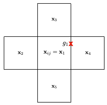
Figure 17: The 5-point GP stencil with a GP radius $R=1$ for the 3rd-order GP-MOOD3 method. One of the two quadrature points, $g_{1}$, is shown with the red cross at the right $x$-directional cell interface of the central cell, $\mathbf{x}_{1}=\mathbf{x}_{ij}$.

Table 4: Tabulated values of $\Delta_{mn,x}$ at each pair of $(\mathbf{x}_{m},\mathbf{x}_{n})$ points.

$\Delta_{mn,d}$	$m=1$	$m=2$	$m=3$	$m=4$	$m=5$	$m=g_{1}$
$n=1$	$0$	$1$	$0$	$-1$	$0$	$-1/2$
$n=2$	$-1$	$0$	$-1$	$-2$	$-1$	$-3/2$
$n=3$	$0$	$1$	$0$	$-1$	$0$	$-1/2$
$n=4$	$1$	$2$	$1$	$0$	$1$	$1/2$
$n=5$	$0$	$1$	$0$	$-1$	$0$	$-1/2$
$n=g_{1}$	$1/2$	$3/2$	$1/2$	$-1/2$	$1/2$	$0$

Table 5: Tabulated values of $\Delta_{mn,y}$ at each pair of $(\mathbf{x}_{m},\mathbf{x}_{n})$ points.

$\Delta_{mn,d}$	$m=1$	$m=2$	$m=3$	$m=4$	$m=5$	$m=g_{1}$
$n=1$	$0$	$0$	$-1$	$0$	$1$	$-\frac{1}{2\sqrt{3}}$
$n=2$	$0$	$0$	$-1$	$0$	$1$	$-\frac{1}{2\sqrt{3}}$
$n=3$	$1$	$1$	$0$	$1$	$2$	$\frac{1}{2}\left(2-\frac{1}{\sqrt{3}}\right)$
$n=4$	$0$	$0$	$-1$	$0$	$1$	$-\frac{1}{2\sqrt{3}}$
$n=5$	$-1$	$-1$	$-2$	$-1$	$0$	$-\frac{1}{2}\left(2+\frac{1}{\sqrt{3}}\right)$
$n=g_{1}$	$\frac{1}{2\sqrt{3}}$	$\frac{1}{2\sqrt{3}}$	$-\frac{1}{2}\left(2-\frac{1}{\sqrt{3}}\right)$	$\frac{1}{2\sqrt{3}}$	$\frac{1}{2}\left(2+\frac{1}{\sqrt{3}}\right)$	$0$

Appendix B GP second derivatives formulas

A GP-based second derivative formula can be derived to compute the second derivatives in Eq. 25. This can be done by differentiating $\mathbf{t}_{*}$ twice in Eq. 14 in each direction, $d=x,y$, since only the prediction vector $\mathbf{t}_{*}$ is affected by the derivative,

$$\frac{\partial^{2}\tilde{m}_{*}}{\partial(\mathbf{e}_{d}\cdot\mathbf{x}_{*})^{2}}=\frac{\partial^{2}\mathbf{t}_{*}^{T}}{\partial(\mathbf{e}_{d}\cdot\mathbf{x}_{*})^{2}}\mathbf{C}^{-1}\mathbf{q}.$$ (44)

The final expression of the GP-based second derivative is written as

$$\frac{\partial^{2}\mathbf{t}_{*,m}^{T}}{\partial(\mathbf{e}_{d}\cdot\mathbf{x}_{*})^{2}} = \prod_{\delta\neq d}\sqrt{\frac{\pi}{2}}\frac{\ell}{\Delta_{\delta}}\left\{\operatorname{erf}\left[\frac{\Delta_{m*,{\delta}}+1/2}{\sqrt{2}\ell/\Delta_{\delta}}\right]-\operatorname{erf}\left[\frac{\Delta_{m*,{\delta}}-1/2}{\sqrt{2}\ell/\Delta_{\delta}}\right]\right\}$$ (45)

$$\times \frac{\partial^{2}}{\partial(\mathbf{e}_{d}\cdot\mathbf{x}_{*})^{2}}\left[\sqrt{\frac{\pi}{2}}\frac{\ell}{\Delta_{d}}\left\{\operatorname{erf}\left[\frac{\Delta_{m*,d}+1/2}{\sqrt{2}\ell/\Delta_{d}}\right]-\operatorname{erf}\left[\frac{\Delta_{m*,d}-1/2}{\sqrt{2}\ell/\Delta_{d}}\right]\right\}\right]$$ (46)

$$= \prod_{\delta\neq d}\sqrt{\frac{\pi}{2}}\frac{\ell}{\Delta_{\delta}}\left\{\operatorname{erf}\left[\frac{\Delta_{m*,{\delta}}+1/2}{\sqrt{2}\ell/\Delta_{\delta}}\right]-\operatorname{erf}\left[\frac{\Delta_{m*,{\delta}}-1/2}{\sqrt{2}\ell/\Delta_{\delta}}\right]\right\}$$ (47)

$$\times \frac{1}{\ell^{2}}\left[\left(\Delta_{m*,d}-\frac{1}{2}\right)\exp\left[-\frac{(\Delta_{m*,d}-\frac{1}{2})^{2}}{2(\ell/\Delta_{d})^{2}}\right]-\left(\Delta_{m*,d}+\frac{1}{2}\right)\exp\left[-\frac{(\Delta_{m*,d}+\frac{1}{2})^{2}}{2(\ell/\Delta_{d})^{2}}\right]\right].$$ (48)

Here, we choose $\mathbf{x}_{*}$ as the center of the cell to obtain the cell-centered second derivative.

Appendix C The full set of coefficients of the 3rd-order polynomial, $p_{3}(x,y)$

The five coefficients, $a_{0},\dots,a_{4}$, of $p_{3}(x,y)$ are obtained by solving Eq. 17, written in terms of $\overline{\mathbf{q}}_{i_{m}j_{m}}$, $1\leq i_{m}j_{m}\leq 5$, as follows:

$$a_{0} = \frac{7}{6}\overline{\mathbf{q}}_{1}-\frac{1}{24}\overline{\mathbf{q}}_{2}-\frac{1}{24}\overline{\mathbf{q}}_{3}-\frac{1}{24}\overline{\mathbf{q}}_{4}-\frac{1}{24}\overline{\mathbf{q}}_{5},$$ (49)

$$a_{1} = -\frac{1}{2}\overline{\mathbf{q}}_{2}+\frac{1}{2}\overline{\mathbf{q}}_{4},$$ (50)

$$a_{2} = -\overline{\mathbf{q}}_{1}+\frac{1}{2}\overline{\mathbf{q}}_{2}+\frac{1}{2}\overline{\mathbf{q}}_{4},$$ (51)

$$a_{3} = \frac{1}{2}\overline{\mathbf{q}}_{3}-\frac{1}{2}\overline{\mathbf{q}}_{5},$$ (52)

$$a_{4} = -\overline{\mathbf{q}}_{1}+\frac{1}{2}\overline{\mathbf{q}}_{3}+\frac{1}{2}\overline{\mathbf{q}}_{5}.$$ (53)

References

- [1] Bram Van Leer. Towards the ultimate conservative difference scheme. ii. monotonicity and conservation combined in a second-order scheme. Journal of computational physics, 14(4):361–370, 1974.
- [2] Eitan Tadmor. Convenient total variation diminishing conditions for nonlinear difference schemes. SIAM journal on numerical analysis, 25(5):1002–1014, 1988.
- [3] ME Hubbard. Multidimensional slope limiters for muscl-type finite volume schemes on unstructured grids. Journal of Computational Physics, 155(1):54–74, 1999.
- [4] Ami Harten. High resolution schemes for hyperbolic conservation laws. Journal of computational physics, 135(2):260–278, 1997.
- [5] Phillip Colella and Paul R Woodward. The piecewise parabolic method (PPM) for gas-dynamical simulations. Journal of computational physics, 54(1):174–201, 1984.
- [6] Peter McCorquodale and Phillip Colella. A high-order finite-volume method for conservation laws on locally refined grids. Communications in Applied Mathematics and Computational Science, 6(1):1–25, 2011.
- [7] Ami Harten and Stanley Osher. Uniformly high-order accurate nonoscillatory schemes. i. In Upwind and High-Resolution Schemes, pages 187–217. Springer, 1997.
- [8] Chi-Wang Shu and Stanley Osher. Efficient implementation of essentially non-oscillatory shock-capturing schemes. Journal of computational physics, 77(2):439–471, 1988.
- [9] Xu-Dong Liu, Stanley Osher, Tony Chan, et al. Weighted essentially non-oscillatory schemes. Journal of computational physics, 115(1):200–212, 1994.
- [10] Guang-Shan Jiang and Chi-Wang Shu. Efficient implementation of weighted ENO schemes. Journal of computational physics, 126(1):202–228, 1996.
- [11] Dinshaw S Balsara and Chi-Wang Shu. Monotonicity preserving weighted essentially non-oscillatory schemes with increasingly high order of accuracy. Journal of Computational Physics, 160(2):405–452, 2000.
- [12] GA Gerolymos, D Sénéchal, and I Vallet. Very-high-order weno schemes. Journal of Computational Physics, 228(23):8481–8524, 2009.
- [13] Doron Levy, Gabriella Puppo, and Giovanni Russo. Compact central weno schemes for multidimensional conservation laws. SIAM Journal on Scientific Computing, 22(2):656–672, 2000.
- [14] Lucian Ivan and Clinton PT Groth. High-order solution-adaptive central essentially non-oscillatory (ceno) method for viscous flows. Journal of Computational Physics, 257:830–862, 2014.
- [15] Matteo Semplice, Armando Coco, and Giovanni Russo. Adaptive mesh refinement for hyperbolic systems based on third-order compact weno reconstruction. Journal of Scientific Computing, 66(2):692–724, 2016.
- [16] Michael Dumbser, Walter Boscheri, Matteo Semplice, and Giovanni Russo. Central weighted eno schemes for hyperbolic conservation laws on fixed and moving unstructured meshes. SIAM Journal on Scientific Computing, 39(6):A2564–A2591, 2017.
- [17] Jianxian Qiu and Chi-Wang Shu. Hermite weno schemes and their application as limiters for runge–kutta discontinuous galerkin method: one-dimensional case. Journal of Computational Physics, 193(1):115–135, 2004.
- [18] Dinshaw S Balsara, Christoph Altmann, Claus-Dieter Munz, and Michael Dumbser. A sub-cell based indicator for troubled zones in rkdg schemes and a novel class of hybrid rkdg+ hweno schemes. Journal of Computational Physics, 226(1):586–620, 2007.
- [19] Dinshaw S Balsara, Sudip Garain, and Chi-Wang Shu. An efficient class of weno schemes with adaptive order. Journal of Computational Physics, 326:780–804, 2016.
- [20] Adam Reyes, Dongwook Lee, Carlo Graziani, and Petros Tzeferacos. A new class of high-order methods for fluid dynamics simulations using gaussian process modeling: One-dimensional case. Journal of Scientific Computing, 76(1):443–480, 2018.
- [21] Adam Reyes, Dongwook Lee, Carlo Graziani, and Petros Tzeferacos. A variable high-order shock-capturing finite difference method with GP-WENO. Journal of Computational Physics, 381:189–217, 2019.
- [22] Steve Reeves, Dongwook Lee, Adam Reyes, Carlo Graziani, and Petros Tzeferacos. An application of gaussian process modeling for high-order accurate adaptive mesh refinement prolongation. arXiv preprint arXiv:2003.08508; Accepted for publication in CAMCoS, 2021.
- [23] James Kent, Christiane Jablonowski, Jared P Whitehead, and Richard B Rood. Determining the effective resolution of advection schemes. part II: Numerical testing. Journal of Computational Physics, 278:497–508, 2014.
- [24] Stéphane Clain, Steven Diot, and Raphaël Loubère. A high-order finite volume method for systems of conservation laws—multi-dimensional optimal order detection (MOOD). Journal of computational Physics, 230(10):4028–4050, 2011.
- [25] Steven Diot, Stéphane Clain, and Raphaël Loubère. Improved detection criteria for the multi-dimensional optimal order detection (MOOD) on unstructured meshes with very high-order polynomials. Computers & Fluids, 64:43–63, 2012.
- [26] Steven Diot, Raphaël Loubère, and Stephane Clain. The multidimensional optimal order detection method in the three-dimensional case: very high-order finite volume method for hyperbolic systems. International Journal for Numerical Methods in Fluids, 73(4):362–392, 2013.
- [27] Steven Diot. La méthode MOOD Multi-dimensional Optimal Order Detection: la première approche a posteriori aux méthodes volumes finis d’ordre très élevé. PhD thesis, Université de Toulouse, Université Toulouse III-Paul Sabatier, 2012.
- [28] Matteo Semplice and Raphaël Loubère. Adaptive-mesh-refinement for hyperbolic systems of conservation laws based on a posteriori stabilized high order polynomial reconstructions. Journal of Computational Physics, 354:86–110, 2018.
- [29] EF Toro, RC Millington, and LAM Nejad. Towards very high order Godunov schemes. In Godunov methods, pages 907–940. Springer, 2001.
- [30] Vladimir A Titarev and Eleuterio F Toro. ADER: Arbitrary high order Godunov approach. Journal of Scientific Computing, 17(1-4):609–618, 2002.
- [31] Vladimir A Titarev and Eleuterio F Toro. ADER schemes for three-dimensional non-linear hyperbolic systems. Journal of Computational Physics, 204(2):715–736, 2005.
- [32] Michael Dumbser, Olindo Zanotti, Raphaël Loubère, and Steven Diot. A posteriori subcell limiting of the discontinuous galerkin finite element method for hyperbolic conservation laws. Journal of Computational Physics, 278:47–75, 2014.
- [33] Michael Dumbser and Raphaël Loubère. A simple robust and accurate a posteriori sub-cell finite volume limiter for the discontinuous galerkin method on unstructured meshes. Journal of Computational Physics, 319:163–199, 2016.
- [34] Alexandre Bourriaud, Raphaël Loubère, and Rodolphe Turpault. A priori neural networks versus a posteriori mood loop: A high accurate 1d fv scheme testing bed. Journal of Scientific Computing, 84(2):1–36, 2020.
- [35] Jing Shi, Changqing Hu, and Chi-Wang Shu. A Technique of Treating Negative Weights in WENO Schemes. Journal of Computational Physics, 175(1):108–127, January 2002.
- [36] Chi-Wang Shu. High-order finite difference and finite volume WENO schemes and discontinuous Galerkin methods for CFD. International Journal of Computational Fluid Dynamics, 17(2):107–118, 2003.
- [37] Dinshaw S Balsara. Divergence-free reconstruction of magnetic fields and weno schemes for magnetohydrodynamics. Journal of Computational Physics, 228(14):5040–5056, 2009.
- [38] P. McCorquodale, P. Ullrich, H. Johansen, and P. Colella. An adaptive multiblock high-order finite-volume method for solving the shallow-water equations on the sphere. Communications in Applied Mathematics and Computational Science, 10(2):121–162, 2015.
- [39] Q. Zhang, H. Johansen, and P. Colella. A fourth-order accurate finite-volume method with structured adaptive mesh refinement for solving the advection-diffusion equation. SIAM Journal on Scientific Computing, 34(2):B179–B201, 2012.
- [40] W. Zhang, A. Almgren, V. Beckner, J. Bell, J. Blaschke, C. Chan, M. Day, B. Friesen, K. Gott, D. Graves, M. Katz, A. Myers, T. Nguyen, A. Nonaka, M. Rosso, S. Williams, and M. Zingale. Amrex: a framework for block-structured adaptive mesh refinement. Journal of Open Source Software, 4(37):1370, 5 2019.
- [41] Sigal Gottlieb and Chi-Wang Shu. Total variation diminishing Runge-Kutta schemes. Mathematics of computation of the American Mathematical Society, 67(221):73–85, 1998.
- [42] Raymond J Spiteri and Steven J Ruuth. A new class of optimal high-order strong-stability-preserving time discretization methods. SIAM Journal on Numerical Analysis, 40(2):469–491, 2002.
- [43] Dongwook Lee, Hugues Faller, and Adam Reyes. The piecewise cubic method (PCM) for computational fluid dynamics. Journal of Computational Physics, 341:230–257, 2017.
- [44] C.E. Rasmussen and C.K.I. Williams. Gaussian Processes for Machine Learning. Adaptive Computation And Machine Learning. MIT Press, 2005.
- [45] C. Bishop. Pattern recognition and machine learning (information science and statistics), 1st edn. 2006. corr. 2nd printing edn. Springer, New York, 2007.
- [46] Bengt Fornberg and Grady Wright. Stable computation of multiquadric interpolants for all values of the shape parameter. Computers & Mathematics with Applications, 48(5-6):853–867, 2004.
- [47] Bengt Fornberg, Elisabeth Larsson, and Natasha Flyer. Stable computations with gaussian radial basis functions. SIAM Journal on Scientific Computing, 33(2):869–892, 2011.
- [48] Bengt Fornberg and Cécile Piret. A stable algorithm for flat radial basis functions on a sphere. SIAM Journal on Scientific Computing, 30(1):60–80, 2008.
- [49] Gregory E Fasshauer and Michael J McCourt. Stable evaluation of gaussian radial basis function interpolants. SIAM Journal on Scientific Computing, 34(2):A737–A762, 2012.
- [50] Bengt Fornberg, Erik Lehto, and Collin Powell. Stable calculation of gaussian-based rbf-fd stencils. Computers & Mathematics with Applications, 65(4):627–637, 2013.
- [51] Grady Barrett Wright. Radial basis function interpolation: numerical and analytical developments. University of Colorado at Boulder, 2003.
- [52] Grady B Wright and Bengt Fornberg. Stable computations with flat radial basis functions using vector-valued rational approximations. Journal of Computational Physics, 331:137–156, 2017.
- [53] Sergei Konstantinovich Godunov. A difference method for numerical calculation of discontinuous solutions of the equations of hydrodynamics. Matematicheskii Sbornik, 89(3):271–306, 1959.
- [54] Dongwook Lee, Adam Reyes, Carlo Graziani, and Petros Tzeferacos. New high-order methods using gaussian processes for computational fluid dynamics simulations. In Journal of Physics: Conference Series, volume 837, page 012018. IOP Publishing, 2017.
- [55] Dinshaw S Balsara and Daniel S Spicer. A staggered mesh algorithm using high order godunov fluxes to ensure solenoidal magnetic fields in magnetohydrodynamic simulations. Journal of Computational Physics, 149(2):270–292, 1999.
- [56] Andrea Mignone, C Zanni, Petros Tzeferacos, B Van Straalen, P Colella, and G Bodo. The pluto code for adaptive mesh computations in astrophysical fluid dynamics. The Astrophysical Journal Supplement Series, 198(1):7, 2011.
- [57] Thomas Padioleau. Development of ”all-régime” AMR simulation methods for fluid dynamics, application in astrophysics and two-phase flows. Theses, Université Paris-Saclay, December 2020.
- [58] Youngjun Lee and Dongwook Lee. A single-step third-order temporal discretization with Jacobian-free and Hessian-free formulations for finite difference methods. Journal of Computational Physics, 427:110063, 2021.
- [59] Youngjun Lee, Dongwook Lee, and Adam Reyes. A recursive system-free single-step temporal discretization method for finite difference methods. Journal of Computational Physics: X, 12:100098, 2021.
- [60] Sigal Gottlieb, David I Ketcheson, and Chi-Wang Shu. Strong stability preserving Runge-Kutta and multistep time discretizations. World Scientific, 2011.
- [61] Eleuterio F Toro, M Spruce, and W Speares. Restoration of the contact surface in the HLL-Riemann solver. Shock Waves, 4(1):25–34, 1994.
- [62] Amiram Harten, Peter D Lax, and Bram van Leer. On upstream differencing and godunov-type schemes for hyperbolic conservation laws. SIAM review, 25(1):35–61, 1983.
- [63] James J Quirk. A contribution to the great riemann solver debate. In Upwind and High-Resolution Schemes, pages 550–569. Springer, 1997.
- [64] Chi-Wang Shu. Essentially non-oscillatory and weighted essentially non-oscillatory schemes for hyperbolic conservation laws. In Advanced numerical approximation of nonlinear hyperbolic equations, pages 325–432. Springer, 1998.
- [65] Chi-Wang Shu and Stanley Osher. Efficient implementation of essentially non-oscillatory shock-capturing schemes, II. In Upwind and High-Resolution Schemes, pages 328–374. Springer, 1989.
- [66] Leonid Ivanovich Sedov. Similarity and dimensional methods in mechanics. CRC press, 1993.
- [67] Bruce Fryxell, Kevin Olson, Paul Ricker, FX Timmes, Michael Zingale, DQ Lamb, Peter MacNeice, Robert Rosner, JW Truran, and H Tufo. FLASH: An adaptive mesh hydrodynamics code for modeling astrophysical thermonuclear flashes. The Astrophysical Journal Supplement Series, 131(1):273, 2000.
- [68] Paul Woodward and Phillip Colella. The numerical simulation of two-dimensional fluid flow with strong shocks. Journal of computational physics, 54(1):115–173, 1984.
- [69] WH Hui, PY Li, and ZW Li. A unified coordinate system for solving the two-dimensional Euler equations. Journal of Computational Physics, 153(2):596–637, 1999.
- [70] Richard Liska and Burton Wendroff. Comparison of several difference schemes on 1D and 2D test problems for the Euler equations. SIAM Journal on Scientific Computing, 25(3):995–1017, 2003.
- [71] Per-Olof Persson. Shock capturing for high-order discontinuous galerkin simulation of transient flow problems. In 21st AIAA computational fluid dynamics conference, page 3061, 2013.
- [72] James M Stone, Kengo Tomida, Christopher J White, and Kyle G Felker. The athena++ adaptive mesh refinement framework: Design and magnetohydrodynamic solvers. The Astrophysical Journal Supplement Series, 249(1):4, 2020.
- [73] Dinshaw S Balsara. Self-adjusting, positivity preserving high order schemes for hydrodynamics and magnetohydrodynamics. Journal of Computational Physics, 231(22):7504–7517, 2012.
- [74] Youngsoo Ha and Carl L Gardner. Positive scheme numerical simulation of high mach number astrophysical jets. Journal of Scientific Computing, 34(3):247–259, 2008.
- [75] Kailiang Wu and Chi-Wang Shu. Provably positive high-order schemes for ideal magnetohydrodynamics: analysis on general meshes. Numerische Mathematik, 142(4):995–1047, 2019.
- [76] Mengqing Liu, Man Zhang, Caixia Li, and Fang Shen. A new locally divergence-free wls-eno scheme based on the positivity-preserving finite volume method for ideal mhd equations. Journal of Computational Physics, page 110694, 2021.
- [77] Dongwook Lee and Anil E Deane. An unsplit staggered mesh scheme for multidimensional magnetohydrodynamics. Journal of Computational Physics, 228(4):952–975, 2009.
- [78] Dongwook Lee. A solution accurate, efficient and stable unsplit staggered mesh scheme for three dimensional magnetohydrodynamics. Journal of Computational Physics, 243:269–292, 2013.
- [79] Nico Fleischmann, Stefan Adami, and Nikolaus A Adams. Numerical symmetry-preserving techniques for low-dissipation shock-capturing schemes. Computers & Fluids, 189:94–107, 2019.