Polycyclic aromatic hydrocarbons and the ionized gas in galaxies with active nuclei

Abstract

We present a study for a sample of galaxies with active nuclei to characterize the main type of PAH molecules present in these objects and the local physical conditions of their irradiating sources, as well as the characteristics of the residing ionized gas, by combining optical and infrared data. Photoionization models were built with the CLOUDY code to reproduce optical emission line ratios in combination with PAH intensity ratios. We find that the species containing 10 $-$ 82 carbon atoms are the most abundant in the sample. We suggest that family of species with only two or three fused rings of and a nitrogen hanging, such as small aromatic amides are important targets worthy of consideration in future experimental/theoretical as well as observational studies. We find that the AGN photoionization models reproduce most of the observational data in the log (6.2/11.3) versus log ([N ii]$\lambda$6584/H$\alpha$) diagram with the optical to X-ray spectral index of $\alpha_{\rm ox}=-1.4$. The flux of small PAH, as well as the flux of ionized PAHs and PANH, decrease as the logarithm of the ionization parameter (log $U$) increases. The 6.2/11.3 PAH intensity ratio presents anti correlation between the oxygen abundance and log $U$, in the sense that the 6.2/11.3 ratio decreases as the oxygen abundance and log $U$ increases. Finally, we found that the ionization degree of PAH species increases with the decreasing of the 11.3/7.7 ratio and the log U, in agreement with the models proposed by Draine & Li .

1 Introduction

Polycyclic Aromatic Hydrocarbons (PAHs) are organic compounds that contain two or more fused benzene rings and can also form large aromatic structures. Although the term PAHs refers to molecules containing only carbon and hydrogen atoms, the more general term "polycyclic aromatic compounds" also includes the functional derivatives, just like nitro-PAHs, Oxy-PAHs, and the heterocyclic analogues. Studies show that PAHs represent one of the most abundant forms of carbon in the Universe, with approximately 15 per cent of the elemental carbon of the Universe is in the form of PAHs (Candian et al., 2018). Besides, PAHs have an important role in heating the Interstellar Medium (ISM) since they have low ionization potential (Tielens, 2008). This class of molecules is often observed in a wide range of astrophysical environments, including extragalactic sources such as Seyferts and Starbursts galaxies (Brandl et al., 2006; Smith et al., 2007; Sales et al., 2010; Sales et al., 2013). They present stronger emission bands at 3.3, 6.2, 7.7, 8.6, 11.2, and 12.7 $\mu$m wavelength (e.g. Li, 2020).

There is an astrobiological interest in PAHs due to their potential role in the formation of protocells, which may help to evaluate possible pathways for the origins of life on the early Earth. Like PAHs, Nitrogen-containing polycyclic aromatic hydrocarbons, known as PANHs, can fragment and form prebiotic molecules, such as ethanol and amino acids (Ehrenfreund et al., 2006). In addition, such species can self-assemble, originating from the formation of protocells (Schrum et al., 2010).

Canelo et al. (2018) analyzed the 6.2 $\mu$m PAH emission band for 155 predominantly starburst-dominated galaxies and distributed it into the Peeters’ A, B and C classes (Peeters et al., 2002), revealing a predominance of 67 per cent of class A sources with band profiles corresponding to a central wavelength near 6.22$\mu$m, which can only be explained by PANHs (Hudgins et al., 2005). In this way, the PANHs, in addition to nitrogen in the gas phase and ices of the ISM, could be another reservoir of nitrogen in the Universe.

Studies have shown that the physical conditions of the object under study at radiation and metallicity levels, for example, affect both approaches. Hanine et al. (2020) found that the size of the formed PAH species increases roughly with increasing temperature up to 800 K, forming rings up to 32 carbon atoms and being correlated with the level of dehydrogenation, which can make these molecules highly reactive (Chen, 2018), characteristic that can intensify the formation of large PAHs.1 Seok et al. (2014), for example, concluded that the PAH abundance is low at low metallicities (Z < 0.1 $Z{{}_{\odot}}$), but increases rapidly beyond a certain metallicity (Z > 0.3 $Z{{}_{\odot}}$) by chemical evolution model in galaxies. On other hand, Maragkoudakis et al. (2018) found that variations on the 17 $\mu$m PAH band depend on the object type, however, there is no dependence on metallicity for both extragalactic H ii regions and galaxies.

PAHs are also important molecules from the galactic diagnosis perspective because their emissions can be used as a calibrator for star formation in galaxies (e.g. Shipley et al. (2016); Maragkoudakis et al. (2018)). Such peculiarity has been a motivating factor for studying the presence of PAHs in active galaxy nuclei (AGNs). Seyfert galaxies are a type of AGNs whose notoriety show presence of PAH emission lines. The ionization of PAH molecules, as well as ionized gas surrounding central engine of the Seyfert galaxies, is dominated by the hardness radiation coming from accreting disk of the supermassive black hole environment. Interestingly, Madden et al. (2006) and Maragkoudakis et al. (2018) have found that the total PAH/Very Small Grains (VSG) intensity ratio decreases with increasing radiation hardness, as traced by [Ne iii]/[Ne ii], indicating that harder radiation fields are largely responsible for the destruction of PAHs in low-metallicity regions. In addition, Sales et al. (2010); Sales et al. (2013) have studied 186 active and star-forming galaxies and could infer that active galaxies seems to present larger PAH molecules ($\geq$ 180 carbon atoms) than starforming galaxies. They propose that PAH molecules can survive near to AGNs since their dusty tori is likely to provide column densities necessary to shield PAHs from the hard radiation field (see also Alonso-Herrero et al., 2014; Ruschel-Dutra et al., 2014).

The nuclear region of the Seyfert and Starburst are excellent objects for studying the signatures of PAHs in order to map the main species of PAHs that are contributing to the emissions in the IR of Seyfert and Starburst galaxies. In additionally, the presence of metallic emission lines, such as [O ii] $\lambda$ 3727, [O iii] $\lambda$ 4363, [O iii] $\lambda$ 4959, [O iii] $\lambda$ 5007, [N ii] $\lambda$ 5755, [N ii] $\lambda$ 6548, [N ii] $\lambda$ 6584, [S ii] $\lambda$ 6717 and [S ii] $\lambda$ 6731, which are present in Seyfert and Starburst galaxies make it possible to estimate the physical conditions (oxygen abundance, density and electronic temperature) of the ionized gas regions. Besides, the ratio of emission lines in combination with photoionization models can be used to determine the hardness of ionizing source and the metallicity of the gas. In this context, it is the possible to verify correlations between the ionized gas regions and the photodissociation regions where PAHs persist.

Concerning the emission features at IR and optical wavelengths, studies have shown (e.g Schkenner (2015)) that large carbon-based molecules (with $\sim$ 10 – 100 atoms) in the gas phase, such as PAHs, long carbon chains or fullerenes should be possible carriers of Diffuse Interstellar Bands (DIBs) and the Unidentified Infrared (UIR) bands. However, the identification of the carriers of DIBs remains to be examined, with the exception of five bands attributed to C${}_{60}^{+}$ Tielens (2013); Campbell et al. (2015). In this sense, the analysis of potential emitting molecules of the PAH population in astrophysical sources in comparison with optical data observed, for instance, can contribute to improving our understanding of those carries and the PAH chemistry in the Universe.

In this paper, we combined optical and infrared data of a sample of Seyfert (Sy) and Starburst (SB) galaxies to characterize the main type of PAH molecules present in these objects and the local physical conditions of their irradiating sources, as well as the characteristics of the residing ionised gas. The paper is organized as follows. In Section 2 we describe the selection of our sample and the data utilized. In the Section 4 and 3 the data analysis is presented. The results and discussions are given in Section 5. The conclusion of the outcome is presented in Section 6.

2 Observational Data and Sample Description

We compiled from the literature a sample of Seyfert and Starburst galaxies with observed and reduced spectra in the infrared and optical. We selected all Starburst and Seyfert galaxies with redshift lower than 0.04 from the Spitzer/IRS ATLAS project (Hernán-Caballero & Hatziminaoglou, 2011) and with low-resolution (R $\sim$ 100) spectra in the range from 5 to 15 $\mu$m, obtained with the Infrared Spectrograph (IRS, Houck et al., 2004) instrument on board the Sptizer Space Telescope (Werner et al., 2004). From this preliminary sample, we chose only objects with optical spectra in the Sloan Digital Sky Survey (SDSS) DR16 (Ahumada et al., 2020). Also, all the selected spectra approximately correspond to nuclear region of the galaxies. All the infrared spectra were obtained in staring-mode, except for Buchanan et al. (2006) and Wu et al. (2009), who utilized the spectral mapping mode, but only the nuclear spectrum was given. We used short-low spectroscopy module covering interval between 5.2$\mu$m and 14.5$\mu$m with a resolving power of R $\sim$ 60-127 and slit size of 3.6 to 3.7 arcseconds per 57 arcseconds.

Table 1: Selected objects and their respective information, including the source’s name, IR reference, nuclear type, equatorial coordinates ($\alpha$ and $\delta$), absolute magnitude in visual band ($M_{\textrm{B}}$), bolometric luminosity in visual band ($L_{\textrm{V}}$) and infrared luminosity $L_{\textrm{IR}}$.

Object	IR Reference	Nuclear Type	$\alpha(2000)^{a}$	$\delta(2000)^{a}$	$z^{a}$	$M_{\textrm{B}}$(mag)a	$L_{\textrm{V}}$ ($L_{\odot}$)a	$L_{\textrm{IR}}$ ($L_{\odot}$)a
Mrk 273	Wu et al. (2009)	Seyfert ${[1]}$	$13^{\rm{h}}44^{\rm{m}}42\aas@@fstack{s}1$	$55^{\rm{h}}53^{\rm{m}}13\aas@@fstack{s}$0	0.038	$-22.34$	8.37$\times 10^{10}$	7.94$\times 10^{10}$
MrK 471	Deo et al. (2007)	Seyfert ${[1]}$	$14^{\rm{h}}22^{\rm{m}}55\aas@@fstack{s}4$	$32^{\rm{h}}51^{\rm{m}}03\aas@@fstack{s}0$	0.034	-22.80	4.58$\times 10^{10}$	4.21$\times 10^{10}$
Mrk 609	Deo et al. (2007)	Seyfert ${[1]}$	$03^{\rm{h}}25^{\rm{m}}25\aas@@fstack{s}3$	$-06^{\rm{h}}08^{\rm{m}}38\aas@@fstack{s}$0	0.034	-22.48	6.58$\times 10^{10}$	4.85$\times 10^{10}$
Mrk 622	Deo et al. (2007)	Seyfert ${[1]}$	$08^{\rm{h}}07^{\rm{m}}41\aas@@fstack{s}0$	$39^{\rm{h}}00^{\rm{m}}15\aas@@fstack{s}0$	0.029	-21.44	3.18$\times 10^{10}$	1.85$\times 10^{10}$
Mrk 883	Deo et al. (2007)	Seyfert ${[1]}$	$16^{\rm{h}}29^{\rm{m}}52\aas@@fstack{s}9$	$24^{\rm{h}}26^{\rm{m}}38\aas@@fstack{s}0$	0.038	-22.19	2.70$\times 10^{10}$	3.95$\times 10^{10}$
NGC 660	Brandl et al. (2006)	LINER ${[1]}$	$01^{\rm{h}}43^{\rm{m}}02\aas@@fstack{s}4$	$13^{\rm{h}}38^{\rm{m}}44\aas@@fstack{s}4$	0.003	-21.50	1.32$\times 10^{10}$	2.02$\times 10^{10}$
NGC 2622	Deo et al. (2007)	Seyfert ${[5]}$	$08^{\rm{h}}38^{\rm{m}}10\aas@@fstack{s}9$	$24^{\rm{h}}53^{\rm{m}}43\aas@@fstack{s}0$	0.023	-22.80	4.75$\times 10^{10}$	6.35$\times 10^{10}$
NGC 2623	Brandl et al. (2006)	Starburst ${[2]}$	$08^{\rm{h}}38^{\rm{m}}24\aas@@fstack{s}1$	$25^{\rm{h}}45^{\rm{m}}16\aas@@fstack{s}9$	0.018	-21.80	3.35$\times 10^{10}$	1.74$\times 10^{11}$
NGC 4676	Brandl et al. (2006)	Starburst ${[3]}$	$12^{\rm{h}}46^{\rm{m}}10\aas@@fstack{s}1$	$30^{\rm{h}}43^{\rm{m}}55\aas@@fstack{s}0$	0.009	-20.97	2.20$\times 10^{10}$	5.15$\times 10^{10}$
NGC 4922	Wu et al. (2009)	Seyfert ${[4]}$	$13^{\rm{h}}01^{\rm{m}}24\aas@@fstack{s}9$	$29^{\rm{h}}18^{\rm{m}}40\aas@@fstack{s}0$	0.024	-22.20	2.75$\times 10^{10}$	…
NGC 5256	Wu et al. (2009)	Seyfert ${[4]}$	$13^{\rm{h}}38^{\rm{m}}17\aas@@fstack{s}5$	$48^{\rm{h}}16^{\rm{m}}37\aas@@fstack{s}0$	0.028	-22.85	5.23$\times 10^{10}$	1.06$\times 10^{11}$
NGC 5347	Buchanan et al. (2006)	Seyfert ${[1]}$	$13^{\rm{h}}53^{\rm{m}}17\aas@@fstack{s}8$	$33^{\rm{h}}29^{\rm{m}}27\aas@@fstack{s}0$	0.008	-20.33	4.65$\times 10^{9}$	3.43$\times 10^{9}$

References: [1] Véron-Cetty & Véron (2003); [2] Keel (1984); [3] Liu & Kennicutt (1995) [4] Rush et al. (1993); [5] Deo et al. (2007).

Note: ^a Taken from the NASA Extragalactic Database (NED).

Table 1 lists the objects selected for this study, including some basic features. The ionizing source of each galaxy was initially taken from the literature. Diagnostic diagrams initially proposed by Baldwin et al. (1981) (e.g., $[\text{O\,{iii}}]/\rm H\beta$ versus $[\text{N\,{ii}}]/\rm H\alpha$, $[\text{O\,{iii}}]/\rm H\beta$ versus $[\text{S\,{ii}}]/\rm H\alpha$, and $[\text{O\,{iii}}]/\rm H\beta$ versus $[\text{O\,{i}}]/\rm H\alpha$), which are commonly known as BPT diagrams are used to distinguish objects ionized by massive stars (SFs), AGN, and Low-ionization nuclear emission-line regions (LINERs). In order to verify the classification of the ionizing source of our sample, we show in Fig. 1 the diagram $[\text{O\,{iii}}]/\rm H\beta$ versus $[\text{N\,{ii}}]/\rm H\alpha$. The black solid curve represents the theoretical upper limit for the star-forming regions proposed by Kewley et al. (2001) and the black dashed curve is the empirical star-forming limit proposed by Kauffmann et al. (2003), hereafter Ke01 and Ka03, respectively. The blue dot-dashed curve represents the Seyfert-LINER dividing line (Ke01). According to Fig. 1, some galaxies presented a different classification from the literature. However, the nuclear region of the galaxies of our sample is ionized by AGN, including the galaxies that are between Ke01 and Ka03 lines, region denominated as composite region, where the object is ionized by SF and AGN. Then, throughout the text, we will refer to our sample of galaxies as AGNs.

The optical data compiled from SDSS were obtained with BOSS Spectrograph attached to 2.5 m telescope at Apache Point Observatory. The spectra range considered is between 3 600 and 10 400 Å , spectral resolution of $R=$ 1 560 at 3 700 Å , $R=$2 270 at 6 000 Å  and the fiber diameter is 3 arcsec.

Fig. 2 shows an optical spectrum of the nuclear region of the Starburst galaxy NGC 4676, where some emission lines are highlighted, and an infrared spectrum for the same galaxy with the main bands of PAHs indicated. All the compiled spectra were reduced and calibrated in flux and wavelength.

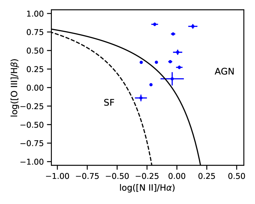
Figure 1: $[\text{O\,{iii}}]/\rm H\alpha$ versus $[\text{N\,{ii}}]/\rm H\alpha$ diagnostic diagram for galaxies of our sample. The black solid curve represents the theoretical upper limit for the star-forming regions proposed by Kewley et al. (2001), and the black dashed curve is the empirical star-forming limit proposed by Kauffmann et al. (2003). The region between the Ke01 and Ka03 lines is denominated composite region.

3 Optical data analysis

The optical spectra from SDSS within the wavelength range of 3 600-10 400 Å  were used to estimate some physical properties of the ionized gas through the use of emission line intensity ratios in combination with photoionization models. The spectrum of each galaxy was processed following the steps listed below:

1. The spectra were corrected to their rest-frame, adopting the values of $z$ listed in Table 1.

2. The pure nebular spectra were obtained after the subtraction of stellar population contribution of the observed spectrum. To obtain the stellar population contribution we use the stellar population synthesis code  STARLIGHT developed by Cid Fernandes et al. (2005); Mateus et al. (2006); Asari et al. (2007). The code fits an observed spectrum with a combination of simple stellar population (SSP) models excluding the emission lines and spurious features (bad pixels or sky residuals). We use the spectral basis of Bruzual & Charlot (2003) with 45 synthetic SSPs spectra with three metallicities, Z = [0.2, 1, and 2.5] Z_⊙, and 15 ages, t = [0.01, 0.003, 0.005, 0.01, 0.025, 0.04, 0.1, 0.3, 0.6, 0.9, 1.4, 2.5, 5, 11, and 13]$\times 10^{9}$ years. The synthetic SSP spectra have a spectral resolution of 3 Å  and to obtain the same spectral resolution of observed spectra these were blended with an elliptical Gaussian function. For more details about the synthesis method see Cid Fernandes et al. (2005), Mateus et al. (2006), and Asari et al. (2007).The flux of the lines in the pure nebular spectra was measuring by using in-house fitting code, which fitting gaussian functions to the line profiles (Hernandez-Jimenez et al., 2013, 2015).

3. The residual extinction associated with the gaseous component for each galaxy was calculated by comparing the observational value for H$\alpha$/H$\beta$ ratio to the theoretical value of 2.86 obtained by Hummer & Storey (1987) for the Case B at electron temperature and density of 10 000 K and 100 cm^-3, respectively. For this, the following expression was considered

   $$\frac{I(\lambda)}{I(\rm H\beta)}=\frac{F(\lambda)}{\rm F(H\beta)}\times 10^{c(\rm H\beta)[f(\lambda)-f(\rm H\beta)]}$$ (1)

   where $I(\lambda)$ is the intensity (reddening corrected) of the emission line at a given wavelength $\lambda$, $F(\lambda)$ is the observed flux of the emission line, $f(\lambda)$ is the adopted reddening curve normalized to $\rm H\beta$, and $c(\rm H\beta$) is the interstellar extinction coefficient.

Table 2 lists the reddening function $f(\lambda)$, the reddening corrected emission line intensities $I(\lambda)$, and the logarithmic extinction coefficient $c(\rm H\beta)$ for each object.

Table 2: Reddening corrected emission-line intensities and the logarithmic extinction coefficient, $c$(H$\beta$). The flux for H$\beta$ and H$\alpha$ are 100 and 286, respectively.

Object	[O iii]$\lambda$4959	[O iii]$\lambda$5007	[N ii]$\lambda$6548	[N ii]$\lambda$6584	[S ii]$\lambda$6716	[S ii]$\lambda$6731	$c$(H$\beta$)
$f(\lambda)$	-0.02	-0.04	-0.35	-0.39	-0.39	-0.43
MrK 273	77$\pm$2	224$\pm$5	87$\pm$2	252$\pm$7	79$\pm$2	65$\pm$2	1.29$\pm$0.02
Mrk 471	226$\pm$10	670$\pm$28	131$\pm$9	389$\pm$24	96$\pm$8	84$\pm$7	0.69$\pm$0.05
Mrk 609	178$\pm$4	529$\pm$11	90$\pm$3	266$\pm$8	49$\pm$2	52$\pm$3	0.67$\pm$0.03
Mrk 622	101$\pm$9	300$\pm$15	98$\pm$6	290$\pm$18	65$\pm$4	56$\pm$4	0.67$\pm$0.05
Mrk 883	73$\pm$1	219$\pm$1	48$\pm$1	144$\pm$2	74$\pm$1	58$\pm$1	0.39$\pm$0.01
NGC 660	66$\pm$4	187$\pm$6	105$\pm$5	300$\pm$13	75$\pm$3	58$\pm$3	1.55$\pm$0.04
NGC 2622	310$\pm$8	947$\pm$23	186$\pm$9	569$\pm$23	175$\pm$10	184$\pm$11	0.04$\pm$0.04
NGC 2623	46$\pm$6	131$\pm$18	91$\pm$14	261$\pm$41	75$\pm$12	58$\pm$9	1.30$\pm$0.14
NGC 4676	25$\pm$3	72$\pm$5	50$\pm$4	143$\pm$12	63$\pm$5	44$\pm$4	1.29$\pm$0.07
NGC 4922	75$\pm$1	220$\pm$2	66$\pm$1	193$\pm$3	50$\pm$1	48$\pm$1	1.00$\pm$0.01
NGC 5256	37$\pm$1	109$\pm$1	58$\pm$1	174$\pm$1	63$\pm$1	58$\pm$1	0.53$\pm$0.01
NGC 5347	239$\pm$8	714$\pm$23	62$\pm$3	186$\pm$9	75$\pm$4	66$\pm$4	0.55$\pm$0.04

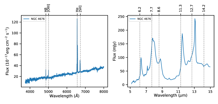
Figure 2: Left panel: the observed optical spectrum for the nuclear region of NGC 4676 obtained with SDSS. Right panel: the observed infrared spectrum for the nuclear region of NGC 4676 obtained with IRS of Spitzer.

3.1 Oxygen abundance and ionization parameter

This section briefly discusses the methods used to estimate the oxygen abundance and the ionization parameter of the ionized gas in the galaxies.

Oxygen is the element widely used as a proxy for global gas-phase metallicity $Z$ (Kennicutt et al., 2003); (Hägele et al., 2008) of gaseous nebulae. This element has prominent emission lines, and their most important ionization stages are present in the optical spectra of these objects. One of the most reliable methods to determine the oxygen abundance is based on the ratio between oxygen forbidden lines and hydrogen lines, and the electron temperature ($T_{\rm e}$), specially for star-forming regions and planetary nebulae. Measurements of the auroral lines, such as [O iii] $\lambda\,4363$, and [N ii] $\lambda\,5755$, are necessary to determine $T_{\rm e}$. Unfortunately, they are very faint and often drop below the detectability level in the spectra of high-metallicity H ii regions. This method is known as the $T_{\rm e}$-method or direct method. Unfortunately, we do not detect temperature-sensitive emission lines [O iii] $\lambda\,4363$, and [N ii] $\lambda\,5755$ in the spectra of the galaxies, and then the direct method could no be used to determine the O/H abundance.

Here, we determine the O/H abundance combining the observed emission line ratios with a grid of photoionization models. The photoionization model grids were built using version 17.02 of the CLOUDY code (Ferland et al., 2017) in order to compare the observational emission-line intensity ratios for the galaxies in our sample with the photoionization model predictions for similar emission-line intensity ratios. The input parameters of the models are briefly described in the following, however, for more details to these parameters see Dors et al. (2015); Dors et al. (2017); Dors et al. (2020) and (Carvalho et al., 2020).

1. The Spectral Energy Distribution (SED): The SED utilized was typical of AGNs, consisting of the sum from the Big Bump component peaking at $\approx$ 1 Ryd, which is parametrized by the temperature of the bump assumed to be $1.5\>\times\>10^{5}$ K and, an X-ray power law with spectral index $\alpha_{\rm x}$ = -1.0, representing the non-thermal X-ray radiation. The continuum between 2 keV and 2500 Å  is described by a power law with the optical to X-ray spectral index $\alpha_{ox}$, which is defined by

   $$\alpha_{ox}=\frac{\log[F(2\>{\rm keV})/F(2500\>\textrm{\AA})]}{\log[\nu(2\>{\rm keV})/\nu(2500\>\textrm{\AA})]},$$ (2)

   where $F$ is the flux at 2 keV, 2500 Å and $\nu$ are the corresponding frequencies (Tananbaum et al., 1979). Therefore, the $\alpha_{\rm ox}$ is the power-law slope connecting the monochromatic flux at 2500 Å  and at 2 keV and display hard X-ray spectra. For instance, SEDs with small values of $\alpha_{\rm ox}$, e.g -2, represent an ionization source with a very soft spectrum yielding models with a very low ionization degree (e.g. 2019MNRAS.486.5853D).

2. Metallicity ($Z$): The metallicities used in relation with the solar value ($Z/Z_{\odot}$) was 0.5, 1.0, 1.5, 2.0, 2.5, 3.0, 3.5 and 4.0. The assumed solar oxygen abundance is 12 + log(O/H)_⊙ = 8.69 (Asplund et al., 2009; Allende Prieto et al., 2001) whose abundances 8.40, 8.69, 8.86, 8.99, 9.08, 9.16, 9.23, and 9.29, correspond to the above listed metallicities, respectively.

3. Ionization Parameter ($U$): The ionization parameter is defined by $U$=${Q}{(\mathrm{H})}/4\pi R^{2}_{0}nc$, where the ${Q}{(\mathrm{H}})$ is the number of ionizing photons emitted per second by the ionizing source, $R_{0}$ is the distance from the ionization source to the inner surface of the ionized gas cloud in cm, $n$ [cm^-3] is the total hydrogen density (ionized, neutral, and molecular), and $c$ is the speed of light in km s^-1. We considered the logarithm of $U$ in the range of -4.0 $\leq$ log$U$ $\leq$ -1, about the same values considered by Feltre et al. (2016) for AGNs.

4. Electron Density: We assumed for the models an electron density value of $N_{\rm e}$= 500 cm^-3, constant in the nebular radius. The electron density ($N_{\rm e}$) derived from the [S ii]$\lambda\,6717/\lambda\,6731$ for our sample of galaxies is in the range of 111 to 922 cm^-3, with a mean density of $N_{\rm e}$= 411 cm^-3.

5. Inner and outer radius: The inner radius of 3 pc was assumed, which is the distance from the ionizing source to the illuminated gas region. It is a typical value for Seyfert galaxies (Balmaverde et al., 2016). The outer radius was assumed to be the one where the electron temperature of the gas reaches 150 K. It is worth to mentioning that studies has found evidences that the inner wall of the dust torus has around several tenths of a parsec from the central engine (e.g. (Xie et al., 2017)). However, models with different combinations of ${Q}{(\mathrm{H}})$, inner radius and $N_{\rm e}$ but that result in the same U are homologous models with about the same predicted emission-line intensities (Bresolin et al., 1999) and (2019MNRAS.486.5853D).

6. PAH: The size distribution for PAHs is given by a power law of the form a^-3.5, where a is the PAH radius and the number of carbon atoms range from 30 to 500, and 10 size bins (Abel et al., 2008).

In order to extend this analysis to other sources with a wider range of metallicities, we included data taken from the sample of the Spitzer Infrared Nearby Galaxies Survey (SINGs) by Smith et al. (2007), in which the 6.2/11.3 and 6.2/7.7 emission ratios were considered. The log([N ii]$\lambda$6584/H$\alpha$) values of this sample were taken from Moustakas et al. (2010). This sample is composed of Seyfert, LINERS and, star forming galaxies.

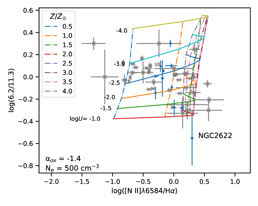
Figure 3: log(6.2/11.3) versus log([N ii]$\lambda$6584/H$\alpha$) diagram. Dashed lines connect photoionization model results with the same metallicity, while solid lines connect models with the same logarithm of the ionization parameter $U$, as indicated. The blue points represent the observational line intensity ratios from the sample considered in this work, and the gray points represent data from Smith et al. (2007). The assumed values of the metallicity ($Z/Z_{\odot}$) and log $U$ values are indicated.

In Fig. 3, a diagram log(6.2/11.3) versus log([N ii]$\lambda$6584/H$\alpha$), the observational data and the photoionization model results obtained with the Cloudy code, assuming $\alpha_{\rm ox}=-1.4$, are shown. It is worth to mention that [N ii$\lambda$6584/H$\alpha$ line ratio is highly sensitive to the metallicity, as measured by the oxygen abundance (O/H) and has a small (although not negligible) ionization parameter dependence (e.g. Kewley et al. 2019; Carvalho et al. 2020). An opposite behaviour is derived for the log(6.2/11.3), which shows a stronger dependence with the ionization degree of the gas (represented by $U$) mainly for the highest values of $U$ rather than with the metallicity. We built grid of models with $\alpha_{ox}=-1.1$ and $-1.4$ and verify that the photoionization model results reproduce the majority of the observed line ratios assuming from the optical to X-ray spectral index $\alpha_{\rm ox}=-1.4$ (see Fig.  3), while for $\alpha_{\rm ox}=-1.1$ (not shown here), there are more points that are not reproduced by the photoionization models. Therefore, we adopted $\alpha_{\rm ox}=-1.4$. This value is representative of typical AGNs, as described in the Hazy manual of the CLOUDY code, and pointed out by Miller et al. (2011); Zhu et al. (2019) and Dors et al. (2019). To calibrate the metallicity as a function of the log(6.2/11.3), we calculated the logarithm of the ionization parameter and the metallicity values for each object of our sample by linear interpolations between the models shown in Fig. 3. Table 3 lists the oxygen abundance and the ionizing parameter $U$ derived by linear interpolation between the models.

Table 3: The oxygen abundance and the ionizing parameter $U$.

Object	12 + log(O/H)⊙	log($U$)
Mrk 273	8.64$\pm$0.01	-3.42$\pm$0.11
Mrk 471	8.83$\pm$0.03	-1.28$\pm$0.23
Mrk 609	8.69$\pm$0.02	-2.08$\pm$0.08
Mrk 622	8.76$\pm$0.04	-1.33$\pm$0.33
Mrk 883	8.62$\pm$0.02	-2.00$\pm$0.33
NGC 660	8.70$\pm$0.01	-2.37$\pm$0.05
NGC 2622	…	…
NGC 2623	8.67$\pm$0.05	-2.62$\pm$0.10
NGC 4676	8.60$\pm$0.02	-2.49$\pm$0.09
NGC 4922	8.63$\pm$0.00	-2.55$\pm$0.05
NGC 5256	8.61$\pm$0.01	-2.69$\pm$0.15
NGC 5347	8.64$\pm$0.03	-2.35$\pm$0.61

4 Infrared Data Analysis

4.1 PAHFIT

The mid-IR spectrum of any object is composed of a diversity of components, such as dust and stellar continuum, emission features from PAHs, forbidden spectral lines from Ne, Ar, S, and Fe, and rotational lines from molecular hydrogen. In low-resolution spectra, these components are blended, and it is necessary to separate them. We employed the spectrum fitting tool PAHFIT (Smith et al., 2007) to decompose the 5 to 15 $\mu$m low-resolution Spitzer’s IRS spectra and obtain the fluxes for different PAH features from our sample.

The default PAHFIT parameters were adopted in the fitting. The dust continuum was represented by blackbodies at fixed temperatures of T = 35, 40, 50, 65, 90, 135, 200, and 300 K. Drude profiles were applied to recover the full strength of dust emission features, with PAH emissions at central wavelengths of 5.3, 5.7, 6.2, 6.7, 7.4, 7.6, 7.7, 7.8, 8.3, 8.6, 10.7, 11.2, 11.3, 12.0, 12.6, 12.7, 13.5, 14.0 and 14.2 $\mu$m. From these measurements, we analyzed the emissions of 6.2 $\mu$m PAH, 7.7 $\mu$m PAH complex, and 11.3 $\mu$m PAH complex. The 7.7$\mu$m PAH complex is the sum of 7.6, 7.7 and 7.8$\mu$m, while 11.3$\mu$m PAH complex is the sum of 11.2 and 11.3 $\mu$m.

The integrated PAH fluxes analyzed in this work are given in Table 4. Fig. 4 shows the detailed decomposition of the starburst galaxy NGC 4676 from 5 to 15 $\mu$m obtained with the PAHFIT code in the components: total continuum, ionic lines, stellar lines, best-fit model, and PAH features. This spectral decomposition was similarly applied to the other eleven objects in our sample.

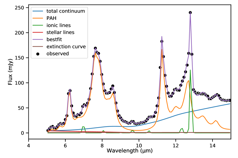
Figure 4: Detailed decomposition of NGC 4676 from 5 to 15 $\mu$m obtained with the PAHFIT code in components of the total continuum, ionic lines, stellar stars, best-fit model, and PAH features.

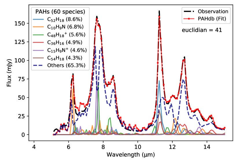
Figure 5: The PAHdb model fitting for the observed spectrum of NGC 4676. The quality of the fitting is quantified by the parameter euclidean. The fractional contribution to the flux from the species is shown.

4.2 PAH spectra

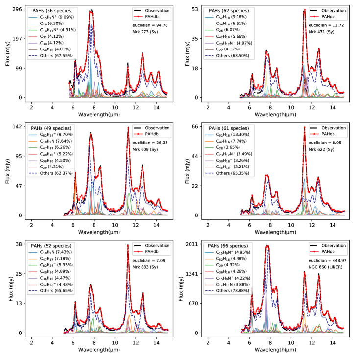
Figure 11: The PAHdb fit to the observed spectrum for the remaining of the objetcs of our sample. The quality of the fitting is quantified by the parameter euclidean. The fractional contribution to the flux from the species is shown.

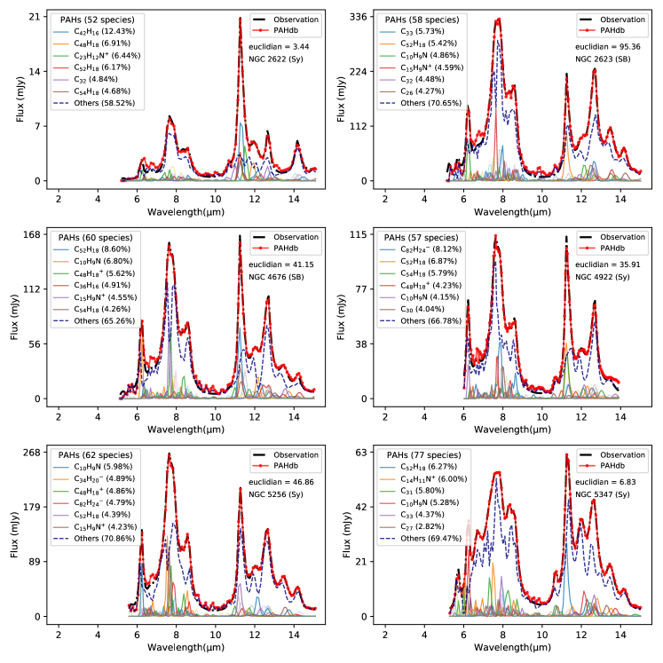
Figure 12: The PAHdb fit to the observed spectrum for the remaining of the objetcs of our sample. The quality of the fitting is quantified by the parameter euclidean. The fractional contribution to the flux from the species is shown.

The PAH spectra of our sample obtained using the PAHFIT were analyzed using version 3.2 of the NASA Ames PAH IR Spectroscopic Database (PAHdb, Boersma et al., 2014; Bauschlicher et al., 2018), which contains 4 233 theoretically calculated PAH spectra. In order to perform the fit, we used the version online of the PAHdb, which is based on spectra of individual aromatic molecules with specific charge states, structures, compositions, and sizes. The Gaussian line profile with a full width at half maximum (FWHM) of 15 cm^-1 and a uniform shift of 15 cm^-1 for all bands was assumed to mimic some effects of anharmonicity. Fig. 5 illustrates the fitting obtained for the spectrum of NGC 4676, and it shows the main species that are contributing to the IR emission in NGC 4676. This fitting resulted in sixty species contributing to the galaxy’s flux. The contributions of the six species that contribute most to the galaxy’s flux are in parenthesis and the their adjusts are showed in different colors. In blue, the contribution of all fifty-four other species. In Fig. 5, it is possible to see the quality of the fit measured by Euclidean norm, whose results are displayed at the top right of the figure. The fitting obtained for the remaining objects is shown in Figs.  11 and 12 (see Appendix B).

5 RESULTS AND DISCUSSION

5.1 Oxygen abundance and the ionization parameter

The effects of the radiation field and metallicity on the intensity ratios and PAH equivalent widths have been reported by many authors in the literature. Due to the significant radiation field of AGNs as revelead by the presence of a significant hot dust continuum, the small PAHs could be destroyed, which tend to decrease the 6.2 and 11.3 $\mu$m intensities (e.g., Sturm et al. 2000; Desai et al. 2007; Diamond-Stanic & Rieke 2010). Smith et al. (2007) performed a study for a sample of Seyfert, LINER and star forming galaxies, and found a trend of the increase of the integrated luminosity of the PAH bands, relative to the total infrared, with the increasing of the oxygen abundance. Besides, these authors verified that the 7.7/11.3 PAH intensity ratio does not vary with the radiation hardness, measured as [Ne iii]/[Ne ii] for star forming galaxies, but shows a dependence for AGNs, specially for [Ne iii]/[Ne ii]> 0.1. However, Maragkoudakis et al. (2018) verified a very weak dependence of the 7.7/6.2 on the hardness of the radiation field and the ionization index for the H i regions along the M 83 and M 33 galaxies (for a review, see for instance, Li 2020).

Table 4: Integrated PAH fluxes (in units of $10^{-16}$ W/m²) obtained by the PAHFIT code.

Object	6.2 $\mu$m	6.7 $\mu$m	7.4 $\mu$m	7.6. $\mu$m	7.8 $\mu$m	8.6 $\mu$m	11.2 $\mu$m	11.3 $\mu$m		12.6 $\mu$m	12.7 $\mu$m
			7.7 $\mu$m Complex				11.3 $\mu$m Complex			12.6 $\mu$m Complex
MrK 273	39.40	36.70	96.60	51.90	82.80	31.40	12.10	7.53		23.10	2.34
Mrk 471	3.79	0.49	0.06	5.60	5.80	3.28	1.42	5.79		3.54	0.26
Mrk 609	15.20	4.76	9.52	24.40	25.40	14.40	3.52	15.30		8.50	1.33
Mrk 622	3.74	1.45	3.59	5.19	5.52	2.95	2.31	4.76		3.81	0.00
Mrk 883	2.97	0.74	0.36	4.22	3.67	1.77	0.96	3.19		1.57	0.36
NGC 660	263.00	112.00	434.00	322.00	496.00	235.00	39.60	216.00		156.00	23.90
NGC 2622	0.59	0.43	0.00	1.57	1.53	0.56	0.58	1.53		0.23	0.22
NGC 2623	46.80	19.20	93.80	51.10	86.80	50.80	12.70	24.40		30.50	4.03
NGC 4676	21.60	7.49	28.30	27.50	31.50	15.40	6.51	14.80		12.30	1.59
NGC 4922	16.00	8.02	21.60	18.40	21.90	10.10	4.04	10.10		7.13	1.23
NGC 5256	32.10	11.10	54.30	41.30	49.10	23.00	7.18	18.50		19.50	0.54
NGC 5347	7.20	10.00	28.80	2.63	8.32	4.79	0.92	6.49		5.99	0.00

Fig. 6 presents the 6.2/11.3 $\mu$m emission ratio as a function of the oxygen abundance (12 + log(O/H)) and the logarithm of the ionization parameter of hydrogen (log $U$) for our sample of galaxies and the SINGs sample by Smith et al. (2007). We notice that the 6.2/11.3 $\mu$m PAH intensity presents a linear correlation with the oxygen abundance, and the ionization parameter $U$. We find the best fit line of 12+ log(O/H) = -0.24$\times$ log(6.2/11.3) + 8.69, with $R=-0.58$, and log($U$) = -3.51$\times$ log(6.2/11.3) - 2.32, with a Pearson correlation coefficient of $R=-0.99$. It is important to emphasize, that for the first time we found that the photoionization models can reproduce most of the observational data in the log (6.2/11.3) versus log([N ii]$\lambda$6584/H$\alpha$) diagram.

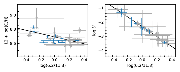
Figure 6: 6.2/11.3 emission ratio as a function of the oxygen abundance (12 + log(O/H)) and the logarithm of the ionization parameter of hydrogen (log $U$). Blue points represent the galaxies of our sample and gray points the SINGs sample of galaxies from Smith et al. (2007). The black solid line is the linear fit to the data.

5.2 Species Identification and Degeneracy

The knowledge on the physico-chemical conditions of the environments where PAHs and PANHs exist is of great importance to understanding the molecular formation and destruction, with the possibility of new compounds being formed. Many issues have been raised about which aromatic species can be found in space environments, while theoretical studies have been conducted out to determine vibration frequencies of potential candidates (Ricca et al., 2019; Mattioda et al., 2020). Also, understanding the link between the evolutionary stage of environments and the aromatic species in them is an enigma that must be studied. In this work, we will call PANH any aromatic molecule composed of carbon, hydrogen and nitrogen, whether nitrogen is inside or outside the ring.

The PAH abundances (PAH %) for each species, i.e., the percentage of the contribution on the flux of each species to the total flux in the spectral range between 5$-$15 $\mu$m, were obtained by dividing the flux contribution of each species by the total flux, which includes the contributions of all species. The total number of species that contribute to IR emission to each galaxy varies from 49 to 77. These species are presented in Appendix C for the twelve studied objects. The most relevant identified species in the sample contain 10 $-$ 82 carbon atoms, while the overall species can be composed of 9 $-$ 170 carbon atoms.

Among the pure hydrocarbons, we highlight the C₅₂H₁₈ (UID 3173), which is present in 75 per cent of the sample and contributes from about 4 per cent to 13 per cent in the galaxy’s fluxes. Among nitrogenous polycyclic aromatic hydrocarbons, C₁₀H₉N (UID 473) is present in 92 per cent of the sample, with fluxes contributions ranging from about 3 to 8 per cent. The molecular ion C₁₀H₉N⁺ is also present in several galaxies analyzed in this work. Similar species such as benzonitrile, also called cyanobenzene (C₆H₅CN), and cyanonaphthalenes (C₁₀H₇N) have already been detected in the dark molecular cloud TMC-1 (McGuire et al., 2018, 2021; McCarthy & McGuire, 2021). Confirmation of hydrocarbons with CN, such as cyanobenzene in TMC-1 and other sources, improves our understanding of chemical processes. Reactions between unsaturated hydrocarbons with CN are usually exothermic and without barrier activation. Furthermore, CN is an abundant radical in most molecular clouds. Since cyan derivatives have significant dipole moments, they are easy targets to detect in radio and, therefore, will have bright rotation spectra (McCarthy & McGuire, 2021).

It is known that there is degeneracy in the fitting of the spectra using the PAHdb database, and it is not possible to guarantee that these three species are always present in the spectra of the galaxies studied here. If C₅₂H₁₈, C₁₀H₉N, and C₁₄H₁₁N are excluded from the database, the PAH spectra can still be reproduced, but the quality of the fitting decreases and the Euclidean have a slightly worse result. In this context, it is worthwhile to known that the species C₁₄H₁₁N, is simply C₁₀H₉N with the addition of one more aromatic ring. This molecule is present in 60 per cent of the sample, and contributes of 2 to 6 per cent of the total flux. For example, the fitting of the spectrum of the galaxy Mrk 273 performed using all database resulted in the contribution of 56 species (see the fitting in Fig. 11), with an Euclidean close to 95. When the species C₅₂H₁₈, C₁₀H₉N, C₁₄H₁₁N and their isomers (15 species) were removed, the PAHdb resulted in 53 species contributing to the galaxy’s flux and the Euclidean value was 108. In this case, some new species were introduced, as well as the relative quantity of the species was slightly modified, when compared with the first fitting (considering all database). However, these new species have the same characteristics of the excluded species, being, majority, small pure PAHs or small PAHs with heteroatom (N or O), with two or three fused aromatic rings. Therefore, although excluded molecules are more appropriate, molecules of the same family also reproduce the spectra of the galaxies, and the presence and (relative) quantity of the PAH species is not uniquely determined.

Then, a coarse, but robust description of the contribution of the types of PAHs of a galaxy may be obtained by grouping their different types. We grouped these types adapted according to Andrews et al. (2015), as dehydrogenated, pure, PANHs, and heteroatom. The table  5 lists the results of flux contribution according to these components.

Table 5: Flux contribution grouped by type of PAHs.

Object	Dehydrogenated	Pure PAHs	PANHs	Heteroatom
	(%)	(%)	(%)	(%)
Mrk 273	42.1	25.1	32.5	0.3
Mrk 471	31.5	53.3	11.9	3.4
Mrk 609	32.2	55.3	10.4	2.0
Mrk 622	36.2	48.9	10.8	4.2
Mrk 883	28.6	60.0	8.3	3.1
NGC 660	33.8	44.3	19.0	3.0
NGC 2622	37.3	51.1	10.8	0.8
NGC 2623	35.2	41.4	23.4	0.0
NGC 4676	30.2	48.9	19.9	1.1
NGC 4992	32.0	49.9	15.9	2.2
NGC 5256	31.6	48.6	19.4	0.4
NGC 5347	47.8	36.2	15.1	1.3

5.3 PANHs and the Peeter Classification

Hudgins et al. (2005) demonstrated that only the nitrogen incorporated into the aromatic rings is capable of reproducing the interstellar observations of the 6.2 $\mu$m PAH band at shorter wavelengths through experimental process. The blueshift of the 6.2 $\mu$m band was also observed in 67 per cent of 155 starburst-dominated galaxies (Canelo et al., 2018). Moreover, Boersma et al. (2013) proposed that the PANH cations dominate both the 6.2 and 11.0 $\mu$m emissions in slightly dense regions of the Photodissociation Region (PDR) known as NGC 7023, and they are also significantly responsible for the emissions of the 7.7, 8.6, 12.0, and 12.7 $\mu$m features.

PANHs, both neutral and cation, generate up to 55 per cent of emission at 6.2 $\mu$m in our sample of galaxies. PANHs also contribute, on average, about 5.7 per cent of the band flux in 11.3 $\mu$m, reaching the value of 37 per cent in the MRK 883.

The importance of N-containing PAHs in the total emission of our sample is also in agreement with the results obtained by Canelo et al. (2018) and Canelo et al. (2021), as can be seen in Table 6. This table shows the Peeters’ classification of the 6.2, 7.7, and 8.6 $\mu$m bands (Peeters et al., 2002), previously obtained by Canelo (2020) to most of our galaxies together with our current classification for NGC 2622, NGC 4922 and NGC 5347. The procedure for this analysis, as well as the new results from those three sources, are described in Appendix D. The 6.2 $\mu$m band, in particular, was mainly distributed into the A class objects, implying a predominance of blue shifted profiles, which are typical of PANH emission and thus confirms the presence of such molecules in these sources.

Besides, we found that the majority of the PAH population is composed of up to 95 per cent of small species (81 per cent being the average) and 79 per cent of neutral PAHs ( 68 per cent the average) in our sample of galaxies. These values are consistent with those provided by Martins-Franco & Menéndez-Delmestre (2021), who found that the predictions by the code PAHdb species of a sample based on Spitzer/IRS mid-infrared spectra of  700 dusty galaxies from the GOALS and ATLAS surveys shown themselves to be predominantly small and neutral PAHs.

In this sense, we can attribute a young object profile to our studied sources with ISM-type environments and a PAH population dominated by small species (Shannon & Boersma, 2019). Therefore, the spectra of our sample are consistent with Peeters’ A class object, which corresponds to H ii regions and the general material illuminated by a star in the ISM. On the other hand, large PAHs are normally more connected with B class spectra of evolved objects, such as circumstellar material, planetary nebula, and a variety of post-AGB (asymptotic giant branch) stars (e.g Tielens, 2008; Andrews et al., 2015; Peeters et al., 2017). Moreover, the B class profiles could also be a mixture of PANH, small and large PAH emissions (Peeters et al., 2002). It is important to note that Yang et al. (2017) suggested that neither PAHs with a large side chain nor PAHs with unsaturated alkyl chains are expected to be present in the ISM in a large abundance. From Table 6, both A and B classes are present in our sample, which emphasizes the importance of spatially-resolved observations in the determinations of which locations in the galaxies where those different PAH populations are more relevant.

Furthermore, Boersma et al. (2013) and Andrews et al. (2015) showed that the dominance of the emissions of small molecules increases with the proximity of the ionizing source. Draine & Li (2001) also demonstrated this behaviour when they proposed that small PAHs emit mainly at 6.2 and 7.7 $\mu$m bands, while large PAHs emit at longer wavelengths (Allamandola et al., 1999). Concerning the neutral species, their predominance is also expected in photodissociation regions where the species can be shielded due to high density/low temperature environments. In fact, Allamandola et al. (1999) demonstrated that the absorption spectrum produced by the neutral PAHs, compared to the spectrum produced by the same PAHs in the cationic form, segregate separately in different regions of the IR when these PAHs are small. According to Bauschlicher et al. (2008), small PAHs emit at 5 – 9 $\mu$m region while the emissions at shorter wavelengths of the 11.3 $\mu$m profile would be produced by neutral PAH molecules.

Table 6: Peeters’ classification of the 6.2, 7.7 and 8.6 $\mu$m PAH bands of the studied galaxies.

Source	6.2 $\mu$m	7.7 $\mu$m	8.6 $\mu$m	Reference
	Class	Class	Class
Mrk 273	A	B	A	[1,2]
MrK 471	B	A	B	[1,2]
Mrk 609	A	B	B	[1,2]
MrK 622	A	A	A	[1,2]
Mrk 883	B	A	A	[1,2]
NGC 660	A	A	A	[1,2]
NGC 2622	B	A	A	This work
NGC 2623	A	B	B	[1,2]
NGC 4676	A	B	A	[1,2]
NGC 4922	A	A	B	This work
NGC 5256	A	A	B	[1,2]
NGC 5347	B	C	…	This work

References: [1] Canelo et al. (2018); [2] (Canelo et al., 2021).

5.4 Small and ionized PAHS, PANHS and the ionization parameter

It is widely known that the size of PAH species and their ionization states can directly be related to the physical conditions of the local environment (Tielens, 2005; Sidhu et al., 2021), in specially of the ionizing field, and a factor of its characterization is the ionization parameter $\log U$.

In this section, we investigate the relation among the contribution of small PAHs, PANHs and ionized PAHs and log $U$. In Fig.  7, we plot these PAH populations as a function of ionization parameter. We can see that the contribution of the small PAHs and PANHs drops as the hydrogen ionization parameter increases (left panel). The correlation is very strong in both cases; with a Pearson coefficient of $R=-0.71$ (P-value$=0.012$) for the PAHs, while the PANHs has a $R=-0.86$ (P-value$=0.0006$). The best linear fit for the former molecules is Flux_(SmallPAHs) = -4.9 log$(U)$ + 68.76, whereas for the latter ones is Flux(PANHs) = -9.9 log $U$ - 5. The main reason for a decrease of the fraction of smaller PAHs and PANHs with increasing ionization factor is due to the fact that the latter factor is directly correlated with the rising of the fragmentation rate of the smaller PAHs and PANHs, since they have lower energy of dissociation than larger PAHs (e.g., Peeters et al., 2005). For example the dissociation energy for the formation of the cation C₃H₃ from the smaller PAH Naphthalene (C₁₀H₈) and aromatic hydrocarbon Benzene (C₆H₆) is 19 eV and 14 eV, respectively (NIST webbook). In addition, the dissociation energy is lower for PANHs than for smaller PAHs (e.g., for dissociation of aromatic hydrocarbon 2-Methylpyridine, C₆H₇N, in the cation C₅H₆ the energy is 12.87 eV), and as most of PANHs in our sample are amides (an amide group outside the ring) the dissociation energy is even lower (e.g., for dissociation of aromatic hydrocarbon Aniline, C₆H₇N, in the cation C₅H₆ the mean energy is 11.96 eV); this explains why the fraction of the smaller PANHs fall ($\sim$35% to $\sim$5%) faster than the PAHs ($\sim$90% to $\sim$75%). Likewise, the lower percentage of PANHs (mean value of 17%) with respect to small PAHs (81%) could be explained by their higher rates of dissociation reducing their half-life time (Peeters et al., 2005). Therefore the fraction of small PAHs and PANHs fall as the U factor increases.

According to O’Dowd et al. (2009), an AGN source preferentially destroys small PAH species with its strong radiation field, favouring the predominance of large species. As a consequence, the environment is more metallically enriched due to the high destruction of small PAHs. The studies by Sales et al. (2010) suggested that Seyferts tend to present an IR emission dominated by PAH molecules with more than 180 carbon atoms, while other objects such as Starbursts normally form molecules with less than 180 carbons. Indeed, the torus can also explain the dominance of the smaller PAHs in our sample, once it can protect the ISM-type environments of galaxies of our sample of the harder radiation field of the central engine. As can be noted, despite of the presence of the AGN these galaxies were classified as starburst-dominated sources, in which class A and B profiles and, consequently, smaller PAHs seem to be presented (e.g. Canelo et al., 2021; Sales et al., 2010; Sales et al., 2013).

The right panel of Fig. 7 also shows that the fraction of ionization of the PAHs decreases as the ionization factor increases. The correlation coefficient is $R=-0.84$ (P-value $=0.001$), and the best liner fit is given by Flux(ionized PAHs) = -11.4 log $U$ + 7.2. This result could be explained whether the PAH fragmentation rate is greater than the ionization rate, then, in this case, the percentage of ionized small PAHs diminishes as the U factor increases. Moreover, Jochims et al. (1994) showed that PAHs containing less than 30-40 carbon atoms, when photoexcited, tend to dissociate rather than relax by infrared emission. In the case of larger PAHs, the main relaxation way will occur via infrared emission (see also Sales et al., 2010; Sales et al., 2013).

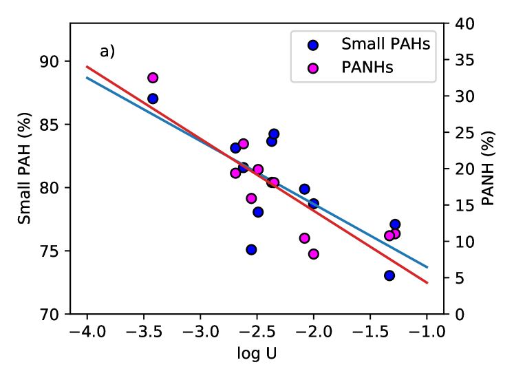
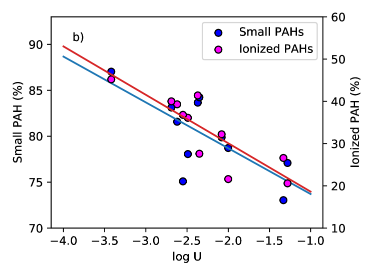
Figure 7: Small PAHs and PANHs versus log $U$ (right) and small PAHs versus log $U$ (left). The red and blue solid lines represent the best fits between the percentage total flux of the species (small, ionized PAHs and PANHs) and log$U$.

In order to verify whether our results agrees with the classical models from Draine & Li (2001), we verified the relation between the percentage of ionization of PAHs determined from the PAHdb with the 11.3/7.7 PAH band strength (observational) and the ionization parameter determined from the photoionization models. It is showed in Fig. 8, and as expected, we see that the ionization degree of PAH species increases with the decreasing of the 11.3/7.7 ratio and the ionization parameter. We found that the Ionized species (%) $=-28.11\log(11.3/7.7)+16.22$, with $R=-0.90$ (P-value=0.0002).

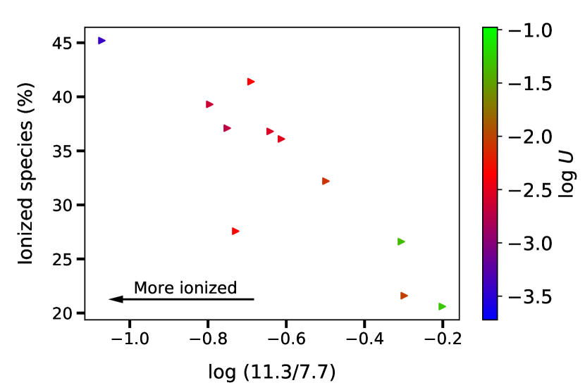
Figure 8: The 11.3/7.7 emission ratios versus ionized species in percentage and log $U$.

6 Conclusions

In this study, we combined optical and infrared data of a sample of Seyfert (Sy) and Starburst (SB) galaxies to characterize the main type of PAH molecules present in these objects and the local physical conditions of their irradiating sources, as well as the characteristics of the residing ionised gas. The infrared data were selected from ATLAS Spitzer/IRS with low-resolution spectra in the 5-15 $\mu$m wavelength range and local redshift, and the optical spectra from the Sloan Digital Sky Survey, DR16, in the wavelength range of 3 600-10 400 Å. Photoionization model grids were built using the CLOUDY code version 17.02 in order to compare the observational emission-line intensity ratios for the galaxies in our sample with the photoionization model predictions for similar emission-line intensity ratios. The main findings are summarised in the following bulletin:

1. Species containing 10 $-$ 82 carbon atoms are the most abundant in the sample, while the overall species can be composed of 9 $-$ 170 carbons;
   

2. Depending on the galaxy in our sample, the PAH population can contain up to 95 per cent of small species (the average being 81 per cent) and 79 per cent of neutral PAHs (the average being 68 per cent);
   

3. Among the pure hydrocarbons, C₅₂H₁₈ deserves the most attention, since it is found in 75 per cent of the sample, contributing from about 5 per cent to 13 per cent in the galaxy’s fluxes;
   

4. Concerning PANHs, these species contribute about 8 $-$ 32 per cent of the total emission in all the studied objects (17 per cent on average). Aromatic amides, such as C₁₀H₉N, C₁₀H₉N⁺, C₁₄H₁₁N and, C₁₅H₉N⁺ are among the most relevant species contributing to the IR emitting flux. C₁₀H₉N is an important species, which is present in 92 per cent of our sample.
   

5. Although it is not possible to guarantee that the aromatic amides mentioned above and C₅₂H₁₈ are always present in the spectra of the galaxies studied here, due to degeneracy, the removal of these molecules showed a worsening in the fit and the addition of molecules from the same family (small PAHs and aromatic amides, plus a small addition of Oxy-PAHs), suggesting that small PANHs are responsible for a large part of the emission of the galaxies in the sample. Thus, we suggest that aromatic amides, as well as theirs cations should be considered in future experimental/theoretical studies and observations, intending to search for their interstellar detection at radio wavelengths;
   

6. For the first time, we show the AGN photoionization models with $\alpha_{\rm ox}=-1.4$, reproducing very well the observed data points in the diagram log(6.2/11.3) versus log([N ii]$\lambda$6584/H$\alpha$);
   

7. The 6.2/11.3 PAH intensity ratio presents a linear anti correlation between the oxygen abundance and log $U$, in the sense that the 6.2/11.3 ratio decreases as the oxygen abundance and log $U$ increases;
   

8. In our sample, the small PAH flux, as well as the ionized PAH and PANH fluxes, exhibit a decrease trend as hydrogen ionization parameter increases. Notice a linear anti correlation between these parameter. We suggest that this bevahior is directly correlated with the rising of the fragmentation rate of the smaller PAHs and PANHs at high U, since they have lower energy of dissociation than larger PAHs. In addition, the dissociation energy is lower for PANHs than for smaller PAHs, according to the observed behaviour, where the fraction of the smaller PANHs fall ( 35% to  5%) faster than the PAHs ( 90% to  75%) at the considered log(U) range. On the other hand, the decreasing of ionized PAHs with the increasing of U factor could be explained whether the PAH fragmentation rate is greater than the ionization rate.

9. We found that the ionization degree of PAH species increases with the decreasing of the 11.3/7.7 ratio and the ionization parameter (log $U$), in agreement with the models proposed by Draine & Li (2001).

7 Data Availability

The data underlying this article will be shared on reasonable request to the corresponding author.

Appendix A PAHFIT spectra decomposition

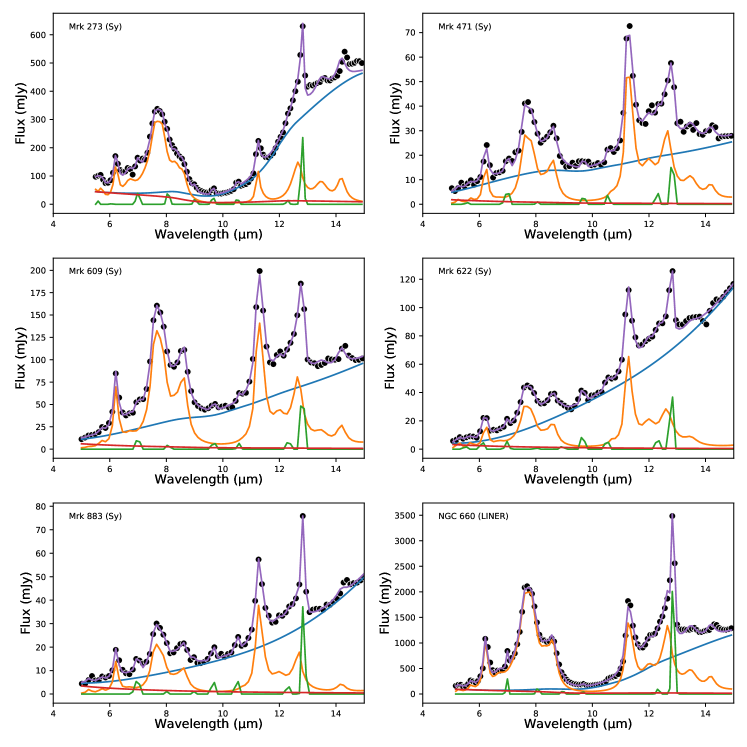
Figure 9: PAHFIT decomposition of our galaxies from 5 to 15 $\mu$m in components of the total continuum (blue line), stellar continuum (red line), ionic lines (green line), PAH and dust features (orange line) and bestfit model (purple line). The data points are shown in black.

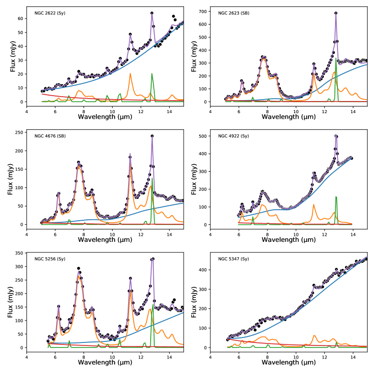
Figure 10: PAHFIT decomposition of our galaxies from 5 to 15 $\mu$m in components of the total continuum (blue line), stellar continuum (red line), ionic lines (green line), PAH and dust features (orange line) and bestfit model (purple line). The data points are shown in black.

Appendix B PAHdb fitting

Appendix C Species emissions each galaxy

Table 7: Species of PAHs that are contributing to the total emission in IR spectrum of Mrk 273. The full table is available online.

UID	Formula	Charge	per cent
470	C15H9N+	1	9.1
2482	C28	0	6.2
480	C14H11N+	1	4.9
2758	C31	0	4.1
2598	C30	0	4.1
⋮	⋮	⋮	⋮

Table 8: Same as Table 7 but for Mrk 471. The full table is available online.

UID	Formula	Charge	per cent
3173	C52H18	0	9.0
836	C54H18	0	6.7
2427	C26	0	6.1
620	C42H16	0	5.7
233	C23H12N+	1	5.0
⋮	⋮	⋮	⋮

Table 9: Same as Table 7 but for Mrk 609. The full table is available online.

UID	Formula	Charge	%
3205	C82H${}_{24}^{-}$	-1	9.7
473	C10H9N	0	7.7
76	C47H17	0	6.2
636	C48H${}_{18}^{+}$	1	5.3
128	C36H16	0	4.5
⋮	⋮	⋮	⋮

Table 10: Same as Table 7 but for Mrk 622. The full table is available online.

UID	Formula	Charge	%
3173	C52H18	0	13.3
620	C42H16	0	7.8
2494	C28	0	3.6
233	C23H12N+	1	3.5
724	C45H${}_{15}^{-}$	-1	3.3
⋮	⋮	⋮	⋮

Table 11: Same as Table 7 but for Mrk 883. The full table is available online.

UID	Formula	Charge	%
76	C47H17	0	7.5
473	C10H9N	0	7.4
3205	C82H${}_{24}^{-}$	-1	6.0
625	C40H16	0	4.9
128	C36H16	0	4.5
⋮	⋮	⋮	⋮

Table 12: Same as Table 7 but for NGC 660. The full table is available online.

UID	Formula	Charge	%
470	C15H9N+	1	5.0
3173	C52H18	0	4.5
2542	C29	0	4.3
128	C36H16	0	4.3
468	C15H9N+	1	4.2
⋮	⋮	⋮	⋮

Table 13: Same as Table 7 but for NGC 2622. The full table is available online.

UID	Formula	Charge	%
620	C42H16	0	13.3
635	C48H18	0	6.8
233	C23H12N+	1	6.8
3173	C52H18	0	6.4
2782	C32	0	4.7
⋮	⋮	⋮	⋮

Table 14: Same as Table 7 but for NGC 2623. The full table is available online.

UID	Formula	Charge	%
2955	C33	0	5.7
3173	C52H18	0	5.4
473	C10H9N	0	4.9
468	C15H9N+	1	4.6
2791	C32	0	4.5
⋮	⋮	⋮	⋮

Table 15: Same as Table 7 but for NGC 4676. The full table is available online.

UID	Formula	Charge	%
3173	C52H18	0	8.6
473	C10H9N	0	6.8
636	C48H${}_{18}^{+}$	1	5.6
128	C36H16	0	4.9
468	C15H9N+	1	4.5
⋮	⋮	⋮	⋮

Table 16: Same as Table 7 but for NGC 4922. The full table is available online.

UID	Formula	Charge	%
3205	C82H${}_{24}^{-}$	-1	8.1
3173	C52H18	0	6.9
836	C54H18	0	5.8
636	C48H${}_{18}^{+}$	1	4.2
473	C10H9N	0	4.1
⋮	⋮	⋮	⋮

Table 17: Same as Table 7 but for NGC 5256. The full table is available online.

UID	Formula	Charge	%
473	C10H9N	0	6.0
822	C34H${}_{20}^{-}$	-1	4.9
636	C48H${}_{18}^{+}$	1	4.9
3205	C82H${}_{24}^{-}$	-1	4.8
3173	C52H18	0	4.4
⋮	⋮	⋮	⋮

Table 18: Same as Table 7 but NGC 5347. The full table is available online.

UID	Formula	Charge	%
3173	C52H18	0	6.3
480	C14H11N+	1	6.0
2758	C31	0	5.8
473	C10H9N	0	5.4
2955	C33	0	4.3
⋮	⋮	⋮	⋮

Appendix D Peeters’ classification procedure

The PAH band profile variations were studied in several astrophysical objects by Peeters et al. (2002), which separated those bands intro three different classes (A, B and C), according to their central wavelengths. The 6 – 9 $\mu$m spectral region, in special, is composed by three PAH main features: a band at 6.2 $\mu$m, a complex of overlapping bands at 7.7 $\mu$m with two components at 7.6 and 7.8 $\mu$m, and a band at 8.6 $\mu$m (Ricca et al., 2018). In the case of the first band, the profile A peaks at shorter wavelengths in comparison to B and C profiles. For the 7.7 $\mu$m complex, the classes A and B differ in the relative strength of the 7.6 and 7.8 $\mu$m features (F_7.6/F_7.8 flux ratio), which seem to be shifted to a peak position of 8.2 $\mu$m for class C objects (Tielens, 2008). Finally, the 8.6 $\mu$m band also peaks at shorter wavelengths for A profiles.

The methodology applied to classify the NGC 2622, NGC 4922 and NGC 5347 galaxies is the same used in the other objects of our sample, previously performed by Canelo et al. (2018), Canelo (2020) and Canelo et al. (2021). The PAHFIT decomposition does not allow the band central wavelengths to vary and can not be used to this analysis. Therefore, we subtracted the underlying continuum with a spline decomposition (e.g. Galliano et al., 2008; Peeters et al., 2017), with a set of anchor points at roughly 5.4, 5.8, 6.6, 7.2, 8.2, 9.0, 9.3, 9.9, 10.2, 10.9, 11.7, 12.1, 13.1, 13.9, 14.7 and 15.0 $\mu$m. In sequence, the 6.2, 7.7 and 8.6 $\mu$m bands were independently fitted with a Gaussian profile (based on the procedure of Peeters et al., 2017, for instance), with a python-based script constructed to estimate their central wavelength ($\lambda_{c}$), amplitude and FWHM through the optimisation algorithms from the submodule scipy.optmize.curve_fit. The uncertainties of these parameters were also derived by this tool with least-squares minimisation from the flux uncertainties provided by the ATLAS. The initial guesses for the parameters were selected from Smith et al. (2007). The continuum and bands fitting are shown in Fig. 13 and Table  19. In the specific case of the 7.7 $\mu$m complex, we fixed the FWHM values according to Peeters et al. (2002) in 0.28 to 7.6 $\mu$m and 0.32 to 7.8 $\mu$m profiles, respectively, to avoid the blending of the features.

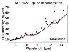
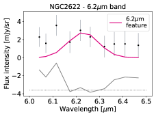
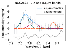
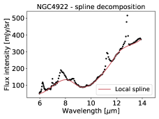
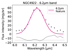
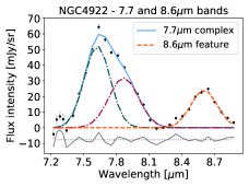
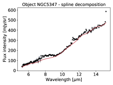
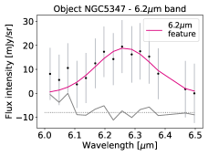
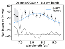
Figure 13: Local spline decomposition and fit results of the 6.2, 7.7 and 8.6 bands for the galaxies of NGC 2622, NGC 4922 and NGC 5347, from top to down. The data points and error bars are in black and grey, respectively.

The particular case of NGC 5347 needed a slightly different approach. The PAH emissions are weaker in this galaxy and the 7 – 10 $\mu$m region resembles an unique bump feature, as expected in class C objects. As a matter of fact, this source was already pointed out as Compton-thick AGN, with a dusty material obscuring the central engine (Kammoun et al., 2019). In order to proper analyse NGC 5347, the anchor point at 8 $\mu$m was not included in the spline decomposition and the 7.7 and 8.6 $\mu$m bands were fitted with just one broad Gaussian profile with peak position at roughly 8.22 $\mu$m (see, for example, Peeters et al., 2002). In such objects, the 7.7 $\mu$m corresponds to a class C object and there is no emission at 8.6 $\mu$m.

With the results of the Gaussian fits, it is possible to separate the sources into the Peeters’ classes. The 6.2 $\mu$m band is considered as class A if $\lambda_{c}$ < 6.23 $\mu$m, class B if 6.23 $\mu$m < $\lambda$ < 6.29 $\mu$m, and class C if $\lambda_{c}$ > 6.29. The 7.7 $\mu$m complex is considered as class A if F_7.6/F_7.8 $\geq$ 1, class B if F_7.6/F_7.8 < 1, and class C if $\lambda_{c}\sim$ 8.22 $\mu$m (the 7.6 and 7.8 $\mu$m features are not present). The 8.6 $\mu$m band does not have a class C profile, and the A and B classifications depend on whether $\lambda_{c}$ < 8.60 $\mu$m or $\lambda_{c}$ > 8.60 $\mu$m, respectively. The classification of NGC 2622, NGC 4922 and NGC 5347 are displayed in Table 6. The F_7.6/F_7.8 ratios of NGC 2622 and NGC 4922 are 2.187 $\pm$ 0.513 and 1.444 $\pm$ 0.134, respectively.

Table 19: Best-fit results for the 6.2, 7.7 and 8.6 $\mu$m bands. A is the amplitude in mJy/sr, $\lambda_{c}$ is the central wavelength in $\mu$m and FWHM is the full width at half maximum.

Source	$\lambda_{c}$	Err	A	Err	FWHM	Err
NGC 2622	6.231	0.011	0.455	0.078	0.153	0.032
	7.653	0.024	1.460	0.171	0.280	—
	7.932	0.051	0.684	0.166	0.320	—
	8.582	0.014	0.413	0.069	0.170	0.033
NGC 4922	6.223	0.002	10.130	0.248	0.159	0.005
	7.625	0.009	15.574	0.845	0.280	—
	7.867	0.014	10.859	0.844	0.320	—
	8.604	0.005	7.271	0.312	0.283	0.015
NGC 5347	6.266	0.007	4.488	0.290	0.223	0.018
	8.221	0.048	43.786	3.868	1.150	0.122

References

- Abel et al. (2008) Abel N. P., van Hoof P. A. M., Shaw G., Ferland G. J., Elwert T., 2008, ApJ, 686, 1125
- Ahumada et al. (2020) Ahumada R., et al., 2020, ApJS, 249, 3
- Allamandola et al. (1999) Allamandola L. J., Hudgins D. M., Sandford S. A., 1999, ApJ, 511, L115
- Allende Prieto et al. (2001) Allende Prieto C., Lambert D. L., Asplund M., 2001, ApJ, 556, L63
- Alonso-Herrero et al. (2014) Alonso-Herrero A., et al., 2014, MNRAS, 443, 2766
- Andrews et al. (2015) Andrews H., Boersma C., Werner M. W., Livingston J., Allamandola L. J., Tielens A. G. G. M., 2015, ApJ, 807, 99
- Asari et al. (2007) Asari N. V., Cid Fernandes R., Stasińska G., Torres-Papaqui J. P., Mateus A., Sodré L., Schoenell W., Gomes J. M., 2007, MNRAS, 381, 263
- Asplund et al. (2009) Asplund M., Grevesse N., Sauval A. J., Scott P., 2009, ARA&A, 47, 481
- Baldwin et al. (1981) Baldwin J. A., Phillips M. M., Terlevich R., 1981, PASP, 93, 5
- Balmaverde et al. (2016) Balmaverde B., Capetti A., Moisio D., Baldi R. D., Marconi A., 2016, A&A, 586, A48
- Bauschlicher et al. (2008) Bauschlicher Charles W. J., Peeters E., Allamandola L. J., 2008, ApJ, 678, 316
- Bauschlicher et al. (2018) Bauschlicher Charles W. J., Ricca A., Boersma C., Allamandola L. J., 2018, ApJS, 234, 32
- Boersma et al. (2013) Boersma C., Bregman J. D., Allamandola L. J., 2013, ApJ, 769, 117
- Boersma et al. (2014) Boersma C., et al., 2014, ApJS, 211, 8
- Brandl et al. (2006) Brandl B. R., et al., 2006, ApJ, 653, 1129
- Bresolin et al. (1999) Bresolin F., Kennicutt Robert C. J., Garnett D. R., 1999, ApJ, 510, 104
- Bruzual & Charlot (2003) Bruzual G., Charlot S., 2003, MNRAS, 344, 1000
- Buchanan et al. (2006) Buchanan C. L., Gallimore J. F., O’Dea C. P., Baum S. A., Axon D. J., Robinson A., Elitzur M., Elvis M., 2006, AJ, 132, 401
- Campbell et al. (2015) Campbell E. K., Holz M., Gerlich D., Maier J. P., 2015, Nature, 523, 322
- Candian et al. (2018) Candian A., Zhen J., Tielens A. G. G. M., 2018, Physics Today, 71, 38
- Canelo (2020) Canelo C. M., 2020, PhD thesis, IAG-USP, Brasil, doi:https://doi.org/10.11606/T.14.2020.tde-03022021-131439
- Canelo et al. (2018) Canelo C. M., Friaça A. C. S., Sales D. A., Pastoriza M. G., Ruschel-Dutra D., 2018, MNRAS, 475, 3746
- Canelo et al. (2021) Canelo C. M., Sales D. A., Friaça A. C. S., Pastoriza M., Menéndez-Delmestre K., 2021, MNRAS, 507, 6177
- Carvalho et al. (2020) Carvalho S. P., et al., 2020, MNRAS, 492, 5675
- Chen (2018) Chen T., 2018, ApJ, 866, 113
- Cid Fernandes et al. (2005) Cid Fernandes R., Mateus A., Sodré L., Stasińska G., Gomes J. M., 2005, Monthly Notices of the Royal Astronomical Society, 358, 363
- Deo et al. (2007) Deo R. P., Crenshaw D. M., Kraemer S. B., Dietrich M., Elitzur M., Teplitz H., Turner T. J., 2007, ApJ, 671, 124
- Desai et al. (2007) Desai V., et al., 2007, ApJ, 669, 810
- Diamond-Stanic & Rieke (2010) Diamond-Stanic A. M., Rieke G. H., 2010, in American Astronomical Society Meeting Abstracts #215. p. 353.05
- Dors et al. (2015) Dors O. L., Cardaci M. V., Hägele G. F., Rodrigues I., Grebel E. K., Pilyugin L. S., Freitas-Lemes P., Krabbe A. C., 2015, MNRAS, 453, 4102
- Dors et al. (2017) Dors O. L. J., Arellano-Córdova K. Z., Cardaci M. V., Hägele G. F., 2017, MNRAS, 468, L113
- Dors et al. (2019) Dors O. L., Monteiro A. F., Cardaci M. V., Hägele G. F., Krabbe A. C., 2019, MNRAS, 486, 5853
- Dors et al. (2020) Dors O. L., Maiolino R., Cardaci M. V., Hägele G. F., Krabbe A. C., Pérez-Montero E., Armah M., 2020, MNRAS, 496, 3209
- Draine & Li (2001) Draine B. T., Li A., 2001, ApJ, 551, 807
- Ehrenfreund et al. (2006) Ehrenfreund P., Rasmussen S., Cleaves J., Chen L., 2006, Astrobiology, 6, 490
- Feltre et al. (2016) Feltre A., Charlot S., Gutkin J., 2016, MNRAS, 456, 3354
- Ferland et al. (2017) Ferland G. J., et al., 2017, Rev. Mex. Astron. Astrofis., 53, 385
- Galliano et al. (2008) Galliano F., Madden S. C., Tielens A. G. G. M., Peeters E., Jones A. P., 2008, ApJ, 679, 310
- Hägele et al. (2008) Hägele G. F., Díaz Á. I., Terlevich E., Terlevich R., Pérez-Montero E., Cardaci M. V., 2008, MNRAS, 383, 209
- Hanine et al. (2020) Hanine M., Meng Z., Lu S., Xie P., Picaud S., Devel M., Wang Z., 2020, ApJ, 900, 188
- Hernán-Caballero & Hatziminaoglou (2011) Hernán-Caballero A., Hatziminaoglou E., 2011, MNRAS, 414, 500
- Hernandez-Jimenez et al. (2013) Hernandez-Jimenez J. A., Pastoriza M. G., Rodrigues I., Krabbe A. C., Winge C., Bonatto C., 2013, MNRAS, 435, 3342
- Hernandez-Jimenez et al. (2015) Hernandez-Jimenez J. A., Pastoriza M. G., Bonatto C., Rodrigues I., Krabbe A. C., Winge C., 2015, MNRAS, 451, 2278
- Houck et al. (2004) Houck J. R., et al., 2004, ApJS, 154, 18
- Hudgins et al. (2005) Hudgins D. M., Bauschlicher Charles W. J., Allamandola L. J., 2005, ApJ, 632, 316
- Hummer & Storey (1987) Hummer D. G., Storey P. J., 1987, MNRAS, 224, 801
- Jochims et al. (1994) Jochims H. W., Ruhl E., Baumgartel H., Tobita S., Leach S., 1994, ApJ, 420, 307
- Kammoun et al. (2019) Kammoun E. S., et al., 2019, ApJ, 877, 102
- Kauffmann et al. (2003) Kauffmann G., et al., 2003, MNRAS, 346, 1055
- Keel (1984) Keel W. C., 1984, ApJ, 282, 75
- Kennicutt et al. (2003) Kennicutt Robert C. J., Bresolin F., Garnett D. R., 2003, ApJ, 591, 801
- Kewley et al. (2001) Kewley L. J., Dopita M. A., Sutherland R. S., Heisler C. A., Trevena J., 2001, ApJ, 556, 121
- Kewley et al. (2019) Kewley L. J., Nicholls D. C., Sutherland R. S., 2019, ARA&A, 57, 511
- Li (2020) Li A., 2020, Nature Astronomy, 4, 339
- Liu & Kennicutt (1995) Liu C. T., Kennicutt Robert C. J., 1995, ApJ, 450, 547
- Madden et al. (2006) Madden S. C., Galliano F., Jones A. P., Sauvage M., 2006, A&A, 446, 877
- Maragkoudakis et al. (2018) Maragkoudakis A., Ivkovich N., Peeters E., Stock D. J., Hemachandra D., Tielens A. G. G. M., 2018, MNRAS, 481, 5370
- Martins-Franco & Menéndez-Delmestre (2021) Martins-Franco Y., Menéndez-Delmestre K., 2021, Astronomische Nachrichten, 342, 186
- Mateus et al. (2006) Mateus A., Sodré L., Cid Fernandes R., Stasińska G., Schoenell W., Gomes J. M., 2006, MNRAS, 370, 721
- Mattioda et al. (2020) Mattioda A. L., et al., 2020, ApJS, 251, 22
- McCarthy & McGuire (2021) McCarthy M. C., McGuire B. A., 2021, Journal of Physical Chemistry A, 125, 3231
- McGuire et al. (2018) McGuire B. A., Burkhardt A. M., Kalenskii S., Shingledecker C. N., Remijan A. J., Herbst E., McCarthy M. C., 2018, Science, 359, 202
- McGuire et al. (2021) McGuire B. A., et al., 2021, Science, 371, 1265
- Miller et al. (2011) Miller B. P., Brandt W. N., Schneider D. P., Gibson R. R., Steffen A. T., Wu J., 2011, ApJ, 726, 20
- Moustakas et al. (2010) Moustakas J., Kennicutt Robert C. J., Tremonti C. A., Dale D. A., Smith J.-D. T., Calzetti D., 2010, ApJS, 190, 233
- O’Dowd et al. (2009) O’Dowd M. J., et al., 2009, ApJ, 705, 885
- Peeters et al. (2002) Peeters E., Hony S., Van Kerckhoven C., Tielens A. G. G. M., Allamandola L. J., Hudgins D. M., Bauschlicher C. W., 2002, A&A, 390, 1089
- Peeters et al. (2005) Peeters Z., Botta O., Charnley S. B., Kisiel Z., Kuan Y. J., Ehrenfreund P., 2005, A&A, 433, 583
- Peeters et al. (2017) Peeters E., Bauschlicher Charles W. J., Allamandola L. J., Tielens A. G. G. M., Ricca A., Wolfire M. G., 2017, ApJ, 836, 198
- Ricca et al. (2018) Ricca A., Bauschlicher C. W., Roser J. E., Peeters E., 2018, ApJ, 854, 115
- Ricca et al. (2019) Ricca A., Roser J. E., Peeters E., Boersma C., 2019, ApJ, 882, 56
- Ruschel-Dutra et al. (2014) Ruschel-Dutra D., Pastoriza M., Riffel R., Sales D. A., Winge C., 2014, MNRAS, 438, 3434
- Rush et al. (1993) Rush B., Malkan M. A., Spinoglio L., 1993, ApJS, 89, 1
- Sales et al. (2010) Sales D. A., Pastoriza M. G., Riffel R., 2010, ApJ, 725, 605
- Sales et al. (2013) Sales D. A., Pastoriza M. G., Riffel R., Winge C., 2013, MNRAS, 429, 2634
- Schkenner (2015) Schkenner S., 2015, Laboratory astrochemistry: From molecules through nanoparticles to grains. Wiley-VCH Verlag
- Schrum et al. (2010) Schrum J. P., Zhu T. F., Szostak J. W., 2010, Cold Spring Harbor Perspectives in Biology, 2
- Seok et al. (2014) Seok J. Y., Hirashita H., Asano R. S., 2014, MNRAS, 439, 2186
- Shannon & Boersma (2019) Shannon M. J., Boersma C., 2019, ApJ, 871, 124
- Shipley et al. (2016) Shipley H. V., Papovich C., Rieke G. H., Brown M. J. I., Moustakas J., 2016, ApJ, 818, 60
- Sidhu et al. (2021) Sidhu A., Peeters E., Cami J., Knight C., 2021, MNRAS, 500, 177
- Smith et al. (2007) Smith J. D. T., et al., 2007, ApJ, 656, 770
- Sturm et al. (2000) Sturm E., Lutz D., Tran D., Feuchtgruber H., Genzel R., Kunze D., Moorwood A. F. M., Thornley M. D., 2000, A&A, 358, 481
- Tananbaum et al. (1979) Tananbaum H., et al., 1979, ApJ, 234, L9
- Tielens (2005) Tielens A. G. G. M., 2005, The Physics and Chemistry of the Interstellar Medium
- Tielens (2008) Tielens A. G. G. M., 2008, ARA&A, 46, 289
- Tielens (2013) Tielens A. G. G. M., 2013, Reviews of Modern Physics, 85, 1021
- Véron-Cetty & Véron (2003) Véron-Cetty M. P., Véron P., 2003, A&A, 412, 399
- Werner et al. (2004) Werner M. W., et al., 2004, ApJS, 154, 1
- Wu et al. (2009) Wu Y., Charmandaris V., Huang J., Spinoglio L., Tommasin S., 2009, ApJ, 701, 658
- Xie et al. (2017) Xie Y., Li A., Hao L., 2017, ApJS, 228, 6
- Yang et al. (2017) Yang X. J., Glaser R., Li A., Zhong J. X., 2017, New Astron. Rev., 77, 1
- Zhu et al. (2019) Zhu S. F., Brandt W. N., Wu J., Garmire G. P., Miller B. P., 2019, MNRAS, 482, 2016