$L_{p}$-Steiner quermassintegrals

Abstract

Inspired by an $L_{p}$ Steiner formula for the $L_{p}$ affine surface area proved by Tatarko and Werner, we define, in analogy to the classical Steiner formula, $L_{p}$-Steiner quermassintegrals. Special cases include the classical mixed volumes, the dual mixed volumes, the $L_{p}$ affine surface areas and the mixed $L_{p}$ affine surface areas. We investigate the properties of the $L_{p}$-Steiner quermassintegrals in a special class of convex bodies. In particular, we show that they are rotation and reflection invariant valuations in this class of convex bodies with a certain degree of homogeneity. Such valuations seem new and have not been observed before.

1 Introduction and Results

An extension of the classical Brunn Minkowski theory, the $L_{p}$ Brunn Minkowski theory, was initiated by Lutwak in the groundbreaking paper [20]. This theory evolved rapidly over the last years and due to a number of highly influential works, see, e.g., [5] - [9], [21] - [28], [30], [39] - [41], it is now a focal part of modern convex geometry. Central objects in the $L_{p}$ Brunn Minkowski theory are the $L_{p}$ affine surface areas,

$$as_{p}(K)=\int_{\partial K}\frac{H_{n-1}(x)^{\frac{p}{n+p}}}{\langle x,N(x)\rangle^{\frac{n(p-1)}{n+p}}}d\mathcal{H}^{n-1}(x),$$

where $N(x)$ denotes the outer unit normal at $x\in\partial K$, the boundary of $K$, $H_{n-1}(x)$ is the Gauss curvature at $x$ and $\mathcal{H}^{n-1}$ is the usual surface area measure on $\partial K$. A missing part in the $L_{p}$ Brunn Minkowski theory was an analog to the classical Steiner formula [4, 29] which says that the volume of the outer parallel body $K+tB^{n}_{2}$ of the convex body $K$ with the Euclidean unit ball $B^{n}_{2}$ is a polynomial in $t$,

$${\rm vol}_{n}(K+tB^{n}_{2})=\sum\limits_{i=0}^{n}{n\choose i}W_{i}(K)t^{i}.$$ (1)

The coefficients $W_{i}(K)$ are the classical quermassintegrals. If the boundary $\partial K$ of the body $K$ is sufficiently smooth, and hence the principal curvatures are well-defined, then $W_{i}(K)=\frac{1}{n}\int_{\partial K}H_{i-1}d\mathcal{H}^{n-1}$, where for $j=1,\dots,n-1$ $H_{j}$ denotes the $j$-th normalized elementary symmetric function of the principal curvatures, see (4).

In [35] an $L_{p}$ Steiner formula was proved for the $L_{p}$ affine surface area. Namely, if $K$ is $C^{2}_{+}$, then we have for all suitable $t$ and for all $p\in\mathbb{R}$, $p\neq-n$, that

$$as_{p}(K+tB^{n}_{2})=\sum\limits_{k=0}^{\infty}\left[\sum\limits_{m=0}^{k}\binom{\frac{n(1-p)}{n+p}}{{k-m}}\mathcal{W}^{p}_{{m},k}(K)\right]t^{k}.$$ (2)

The coefficients $\mathcal{W}^{p}_{{m},k}(K)$ are called $L_{p}$ Steiner coefficients and defined for a (general) convex body $K$ in $\mathbb{R}^{n}$, for all $k,m\in\mathbb{N}\cup\{0\}$ as

$$\hskip-31.29802pt\mathcal{W}^{p}_{m,\,k}(K)=$$

$$\hskip-31.29802pt\int\limits_{\partial K}\langle x,N(x)\rangle^{m-k+\frac{n(1-p)}{n+p}}H_{n-1}^{\frac{p}{n+p}}\sum_{\begin{subarray}{c}i_{1},\dots,i_{n-1}\geq 0\\ i_{1}+2i_{2}+\dots+(n-1)i_{n-1}=m\end{subarray}}c(n,p,i(m))\prod\limits_{j=1}^{n-1}{n-1\choose j}^{i_{j}}H_{j}^{i_{j}}\,d\mathcal{H}^{n-1}.$$

The $c(n,p,i(m))$ are certain binomial coefficients, see (18) for the details. The $\mathcal{W}^{p}_{m,\,k}$ involve integration on $\partial K$. We also define corresponding expressions $\mathcal{Z}^{p}_{m,\,k}$ in (3.2) as integrals over the sphere. If $K$ is sufficiently smooth, we can pass from one expression to the other via the Gauss map. It was also shown in [35] that for $p=0$ the above formula gives the classical Steiner formula (1). In particular, the sum appearing in (2) is then a finite sum. The sum is also finite for all $p=-\frac{n(l-1)}{l}$, $l\in\mathbb{N}$, [35]. In general, the sum is infinite and thus proving (2) requires a careful analysis of convergence issues. Moreover, (2) also includes the Steiner formula for the Minkowski outer parallel body of the dual Brunn Minkowski theory of Lutwak [17] as a special case. In this paper we define in analogy to the classical Steiner formula, for a general convex body $K$ in $\mathbb{R}^{n}$ the $L_{p}$-Steiner quermassintegrals, or $L_{p}$-Steiner mixed volumes as

$$\mathcal{V}^{p}_{k}(K)=\sum\limits_{m=0}^{k}\binom{\frac{n(1-p)}{n+p}}{{k-m}}\mathcal{W}^{p}_{{m},k}(K).$$ (3)

If $p=0$, then the $L_{p}$-Steiner quermassintegrals (3) are the above classical quermassintegrals $W_{i}(K)$ (see [4, 29]) and if $p=\pm\infty$, they are Lutwak’s dual quermassintegrals [17, 19]. Moreover, the $L_{p}$ mixed affine surface areas of Lutwak [18], see also [39], are special cases of the $L_{p}$-Steiner quermassintegrals. The $L_{p}$ Steiner coefficients $\mathcal{W}^{p}_{m,\,k}$ and the $L_{p}$-Steiner quermassintegrals $\mathcal{V}^{p}_{k}$ are complicated expressions, and one needs to clarify when they are well-defined. In Section 3 we introduce a class of convex bodies, the class $\mathcal{C}^{n}$, for which this is the case. We then investigate in detail the properties of the $L_{p}$-Steiner quermassintegrals. Remarkably, it turns out that they are new valuations, which seem not to have been observed before. Valuations on convex sets can be considered as a generalization of the notion of a measure and thus are important quantities in the study of convex sets. Examples of valuations which are not measures in the usual sense are the quermassintegrals and the $L_{p}$ affine surface areas. Due to their importance, much work has been devoted to the study of valuations. Often additional properties like continuity with respect to the Hausdorff metric and invariance under e.g., rigid motions are prescribed. Such valuations have been completely classified in a remarkable theorem by Hadwiger as linear combinations of the quermassintegrals in [10]. For a simpler proof, see [12]. Subsequently, one direction of study in the theory of valuations concentrated on characterization theorems when one successively relaxes the requirements. For instance, upper semi continuous, $GL(n)$-invariant valuations have been characterized by Ludwig and Reitzner [16], involving, in particular, affine surface area. The following theorem combines some of our main results, namely (parts of) Theorems 5.1 and 5.5 below. The class $\mathcal{C}^{n}$ is defined in Section 3. Theorem

Let $K$ be a convex body in $\mathcal{C}^{n}$ and let $p\in\mathbb{R}$ be such that $p\geq 0$ or $p<-n$. . Then we have for all $k\in\mathbb{N}$

• $\mathcal{V}^{p}_{k}$ is homogeneous of degree $n\frac{n-p}{n+p}-k$.

• $\mathcal{V}^{p}_{k}$ is invariant under rotations and reflections.

• $\mathcal{V}^{p}_{k}$ are valuations on the set $\mathcal{C}^{n}$.

In the next two corollaries we list a few consequences of our main theorem. When $p=1$, the expressions $\mathcal{V}^{p}_{k}$ simplify and we denote $\mathcal{V}^{1}_{k}=\mathcal{W}^{1}_{k,\,k}=\mathcal{W}_{k,\,k}$. Additionally to the rotation and reflection invariance, one has translation invariance for $\mathcal{W}_{k,\,k}$. Corollary

For all $k\in\mathbb{N}$, $\mathcal{V}^{1}_{k}=\mathcal{W}_{k,\,k}$ are rigid motion invariant, $n\frac{n-1}{n+1}-k$ homogeneous valuations. For $m=0$, the $\mathcal{W}^{p}_{{m},k}$ are in addition upper or lower semi continuous (depending on the range of $p$). As these coincide with the mixed $L_{p}$ affine surface areas $as_{p+\frac{k}{n}(n+p),-k}$, this shows continuity properties of the latter, which, as far as we know, had not been noted before. Corollary

For $p\geq 0$, $\mathcal{W}^{p}_{0,\,k}=as_{p+\frac{k}{n}(n+p),-k}$ are upper semi continuous $n\frac{n-p}{n+p}-k$ homogeneous valuations that are invariant under rotations and reflections. In view of these corollaries, we remark that a characterization of rigid motion invariant upper semi continuous valuations has been given so far only in the plane [13]. Because of the last corollary and the fact that the $L_{p}$ affine surface areas are semi continuous, it is natural to ask about continuity properties of the $\mathcal{V}^{p}_{k}$ and $\mathcal{W}^{p}_{{m},k}$. We show in Section 5.3 that in general we cannot expect any semi continuity properties.

A byproduct of our analysis is following combinatorial formula. It may be known, but we did not find a reference for it. Corollary

Let $p\in\mathbb{R}$, $p\neq-n$ and $k\in\mathbb{N}\cup\{0\}$. Then

$${n\frac{n-p}{n+p}\choose k}=\sum\limits_{m=0}^{k}\binom{\frac{n(1-p)}{n+p}}{k-m}\sum_{\begin{subarray}{c}i_{1},\dots,i_{n-1}\geq 0\\ i_{1}+2i_{2}+\dots+(n-1)i_{n-1}=m\end{subarray}}c(n,p,i(m))\prod\limits_{j=1}^{n-1}{n-1\choose j}^{i_{j}}$$

where $c(n,p,i(m))$ are certain binomial coefficients, see (18) for the details.

2 Background

2.1 Background from differential geometry

For more information and the details in this section we refer to e.g., [4, 29].

For a point $x$ on the boundary $\partial K$ of $K$ we denote by $N(x)$ an outward unit normal vector of $K$ at $x.$ Occasionally, we use $N_{K}(x)$ to emphasize that it is the normal vector of a body $K$ at $x\in\partial K$. The map $N:\partial K\to S^{n-1}$ is called the spherical image map or Gauss map of $K$ and it is of class $C^{1}.$ Its differential is called the Weingarten map. The eigenvalues of the Weingarten map are the principal curvatures $k_{i}(x)$ of $K$ at $x.$

The $j$-th normalized elementary symmetric functions of the principal curvatures are denoted by $H_{j}$. They are defined as follows

$$H_{j}={n-1\choose j}^{-1}\sum_{1\leq i_{1}<\dots<i_{j}\leq n-1}k_{i_{1}}\cdots k_{i_{j}}$$ (4)

for $j=1,\dots,n-1$ and $H_{0}=1.$ Note that

$$H_{1}=\frac{1}{n-1}\sum_{1\leq i\leq n-1}k_{i}$$

is the mean curvature, that is the average of principal curvatures, and

$$H_{n-1}=\prod_{i=1}^{n-1}k_{i}$$

is the Gauss curvature.

We say that $K$ is of class $C^{2}_{+}$ if $K$ is of class $C^{2}$ and the Gauss map $N$ is a diffeomorphism. This means in particular that $N$ has a smooth inverse. This is stronger than just $C^{2},$ and is equivalent to the assumption that all principal curvatures are strictly positive, or that the Gauss curvature $H_{n-1}>0.$ It also means that the differential of $N$, i.e., the Weingarten map, is of maximal rank everywhere.

Let $K$ be of class $C^{2}_{+}$. For $u\in\mathbb{R}^{n}\setminus\{0\}$, let $\xi_{K}(u)$ be the unique point on the boundary of $K$ at which $u$ is an outward normal vector. The map $\xi_{K}$ is defined on $\mathbb{R}^{n}\setminus\{0\}$. Its restriction to the sphere $S^{n-1}$ is called the reverse spherical image map, or reverse Gauss map, $N_{K}^{-1}:S^{n-1}\to\partial K$. The differential of $N_{K}^{-1}$ is called the reverse Weingarten map. The eigenvalues of the reverse Weingarten map are called the principal radii of curvature $r_{1},\dots,r_{n-1}$ of $K$ at $u\in S^{n-1}.$

The $j$-th normalized elementary symmetric functions of the principal radii of curvature are denoted by $s_{j}$. In particular, $s_{0}=1$, and for $1\leq j\leq n-1$ they are defined as

$$s_{j}={n-1\choose j}^{-1}\sum_{1\leq i_{1}<\dots<i_{j}\leq n-1}r_{i_{1}}\cdots r_{i_{j}}.$$ (5)

Note that the principal curvatures are functions on the boundary of $K$ and the principal radii of curvature are functions on the sphere.

Now we describe the connection between $H_{j}$ and $s_{j}.$ For a body $K$ of class $C^{2}_{+}$, the principal radii of curvature are reciprocals of the principal curvatures, that is

$$r_{i}(u)=\frac{1}{k_{i}(N_{K}^{-1}(u))}.$$

This implies that for $x\in\partial K$ with $N(x)=u$,

$$s_{j}={n-1\choose j}^{-1}\sum_{1\leq i_{1}<\dots<i_{j}\leq n-1}\frac{1}{k_{i_{1}}(N_{K}^{-1}(u))\cdots k_{i_{j}}(N_{K}^{-1}(u))}=\frac{H_{n-1-j}}{H_{n-1}}\Big{(}N_{K}^{-1}(u)\Big{)}$$

and

$$H_{j}=\frac{s_{n-1-j}}{s_{n-1}}\Big{(}N(x)\Big{)},$$

for $j=1,\dots,n-1.$

The mixed volumes $W_{i}(K)$ of the classical Steiner formula (1) can be expressed via the elementary symmetric functions of the principal curvatures. By definition, $W_{0}(K)={\rm vol}_{n}(K)$ and

$$W_{i}(K)=\frac{1}{n}\int\limits_{\partial K}H_{i-1}d\mathcal{H}^{n-1},$$ (6)

for $i=1,\dots,n.$ The dual mixed volume of the convex bodies $K$ and $L$ that contain $0$ in their interiors, introduced by Lutwak [17], is defined for all real $i$ by

$$\widetilde{V}_{i}(K,L)=\frac{1}{n}\ \int\limits_{S^{n-1}}\rho_{K}(u)^{n-i}\rho_{L}(u)^{i}d\sigma(u),$$

where $\rho_{K}(u)=\max\{\lambda\geq 0|\,\lambda u\in K\}$ is the radial function of $K.$ In particular, if $L=B^{n}_{2}$, then

$$\widetilde{W}_{i}(K)=\widetilde{V}_{i}(K,B^{n}_{2})=\frac{1}{n}\int\limits_{S^{n-1}}\rho_{K}(u)^{n-i}d\sigma(u)$$ (7)

are called dual quermassintegrals of order $i.$ The corresponding Steiner formula in the dual Brunn Minkowski theory proved in [17] is

$${\rm vol}_{n}(K\,\widetilde{+}\,tB^{n}_{2})=\sum\limits_{i=0}^{n}{n\choose i}\widetilde{W}_{i}(K)\ t^{i}.$$

2.2 Background from affine geometry

We denote by $\mathcal{K}^{n}_{o}$ the set of all convex bodies in $\mathbb{R}^{n}$ containing the origin $o$. From now on, we will always assume that $K\in\mathcal{K}^{n}_{o}$. For real $p\neq-n$, we define the $L_{p}$ affine surface area $as_{p}(K)$ of $K$ as in [17] ($p>1$) and [33] ($p<1,\ p\neq-n$) by

$$as_{p}(K)=\int\limits_{\partial K}\frac{H_{n-1}(x)^{\frac{p}{n+p}}}{\langle x,N(x)\rangle^{\frac{n(p-1)}{n+p}}}\,d\mathcal{H}^{n-1}(x)$$ (8)

and

$$as_{\pm\infty}(K)=\int\limits_{\partial K}\frac{H_{n-1}(x)}{\langle x,N(x)\rangle^{n}}d\mathcal{H}^{n-1}(x)$$ (9)

provided the above integrals exist. Note that these expressions are not always finite. For example, if $K$ is a polytope and $-n<p<0$, then $as_{p}(K)=\infty$.

In particular, for $p=0$,

$$as_{0}(K)=\int\limits_{\partial K}\langle x,N(x)\rangle\,d\mathcal{H}^{n-1}(x)=n\,{\rm vol}_{n}(K).$$ (10)

The case $p=1$,

$$as_{1}(K)=\int\limits_{\partial K}H_{n-1}(x)^{\frac{1}{n+1}}d\mathcal{H}^{n-1}(x)$$

is the classical affine surface area which is independent of the position of $K$ in space. For dimensions 2 and 3 and sufficiently smooth convex bodies, its definition goes back to Blaschke [2].

If the boundary of $K$ is sufficiently smooth, then (8) and (9) can be written as integrals over the boundary $\partial B^{n}_{2}=S^{n-1}$ of the Euclidean unit ball $B^{n}_{2}$ in $\mathbb{R}^{n}$,

$$as_{p}(K)=\int\limits_{S^{n-1}}\frac{f_{K}(u)^{\frac{n}{n+p}}}{h_{K}(u)^{\frac{n(p-1)}{n+p}}}d\mathcal{H}^{n-1}(u),$$ (11)

where $f_{K}(u)$ is the curvature function, i.e. the reciprocal of the Gaussian curvature $H_{n-1}(x)$ at this point $x\in\partial K$ that has $u$ as outer normal, and $h_{K}(u)=\sup\{\langle x,u\rangle:x\in K\}$, $u\in\mathbb{R}^{n}\setminus\{0\}$, is the support function of $K$. In particular, for $p=\pm\infty$,

$$as_{\pm\infty}(K)=\int\limits_{S^{n-1}}\frac{1}{h_{K}(u)^{n}}d\mathcal{H}^{n-1}(x)=n\,{\rm vol}_{n}(K^{\circ}),$$ (12)

where $K^{\circ}=\{y\in\mathbb{R}^{n}:\langle x,y\rangle\leq 1\ \text{for all }x\in K\}$ is the polar body of $K$. For $p=-n$, the $L_{-n}$ affine surface area was introduced in [26] as

$$as_{-n}(K)=\max_{u\in S^{n-1}}f_{K}(u)^{\frac{1}{2}}h_{K}(u)^{\frac{n+1}{2}}.$$ (13)

Hug [11] proved that (8) and (11) coincide for $p>0$.

3 $L_{p}$ Steiner quermassintegrals

3.1 Definitions

We will need the generalized binomial coefficients. For $\alpha\in\mathbb{R}$ and $k\in\mathbb{N}$, they are defined as

$${\alpha\choose k}=\left\{\begin{aligned} &1\quad&\text{ if }\ k=0,\\ &0\quad&\text{ if }\,k<0\,&\text{ or }\,\alpha=0,\\ &\frac{\alpha(\alpha-1)\cdots(\alpha-k+1)}{k!}\quad&\text{ if }k>0.\end{aligned}\right.$$ (14)

It was shown in [35] that the following $L_{p}$ Steiner formulas hold. They are a generalization of the classical Steiner formula, which corresponds to the case $p=0$ and Lutwak’s Steiner formula of the dual Brunn Minkowski theory, which corresponds to the case $p=\pm\infty$:

Theorem 3.1

[35] Let $k,m\in\mathbb{N}\cup\{0\}$, and $p\in\mathbb{R}$, $p\neq-n$. If $K\in\mathcal{K}_{o}^{n}$ is $C^{2}_{+}$, then we have for all $0\leq t\leq\min\limits_{u\in S^{n-1}}h_{K}(u)$,

$$as_{p}(K+tB^{n}_{2})=\sum\limits_{k=0}^{\infty}\left[\sum\limits_{m=0}^{k}\binom{\frac{n(1-p)}{n+p}}{{k-m}}\mathcal{W}^{p}_{{m},k}(K)\right]t^{k}=\sum\limits_{k=0}^{\infty}\left[\sum\limits_{m=0}^{k}\binom{\frac{n(1-p)}{n+p}}{k-m}\mathcal{Z}^{p}_{m,\,k}(K)\right]t^{k}.$$ (15)

A convex body $K$ has a unique outer normal almost everywhere, and by a theorem of Alexandroff [1] and Busemann-Feller [3] the generalized second partial derivatives exist almost everywhere. Therefore, we extend the definition of the $L_{p}$ Steiner coefficients from smooth convex bodies [35] to general convex bodies $K$.

Definition 3.2 ($L_{p}$-Steiner coefficients)

Let $K\in\mathcal{K}_{o}^{n}$, $k,m\in\mathbb{N}\cup\{0\}$, and $p\in\mathbb{R}$, $p\neq-n$. Then we define

$$\hskip-31.29802pt\,\,\mathcal{W}^{p}_{m,\,k}(K)=$$

$$\hskip-31.29802pt\int\limits_{\partial K}\langle x,N(x)\rangle^{m-k+\frac{n(1-p)}{n+p}}H_{n-1}^{\frac{p}{n+p}}\sum_{\begin{subarray}{c}i_{1},\dots,i_{n-1}\geq 0\\ i_{1}+2i_{2}+\dots+(n-1)i_{n-1}=m\end{subarray}}c(n,p,i(m))\prod\limits_{j=1}^{n-1}{n-1\choose j}^{i_{j}}H_{j}^{i_{j}}\,d\mathcal{H}^{n-1}$$ (16)

and

$$\hskip-31.29802pt\,\,\mathcal{Z}^{p}_{m,\,k}(K)=$$

$$\hskip-31.29802pt\int\limits_{S^{n-1}}h_{K}^{m-k+\frac{n(1-p)}{n+p}}\,s_{n-1}^{\frac{n}{n+p}}(u)\sum_{\begin{subarray}{c}i_{1},\dots,i_{n-1}\geq 0\\ i_{1}+2i_{2}+\dots+(n-1)i_{n-1}=m\end{subarray}}c(n,p,i(m))\frac{\prod\limits_{j=1}^{n-1}{n-1\choose j}^{i_{j}}s_{n-1-j}^{i_{j}}\left(u\right)}{s_{n-1}^{\sum\limits_{j}i_{j}}(u)}\,d\mathcal{H}^{n-1}.$$ (17)

There we have put

$$c(n,p,i(m))={\frac{n}{n+p}\choose i_{1}+\dots+i_{n-1}}{i_{1}+\dots+i_{n-1}\choose i_{1},\,i_{2},\,\ldots,i_{n-1}},$$ (18)

where the sequence $i(m)=\{i_{j}\}_{j=1}^{n-1}$ is such that $i_{1}+2i_{2}+\dots+(n-1)i_{n-1}=m$, and

$${q\choose i_{1},i_{2},\dots,i_{l}}=\frac{q!}{i_{1}!i_{2}!\cdots i_{l}!}$$

is the multinomial coefficient where $q=i_{1}+\dots+i_{l}$. Note that

$${q\choose i_{1},i_{2},\dots,i_{l}}=0\quad\text{ if }\ i_{j}<0\text{ or }i_{j}>q.$$

When $l=2,$ we get the binomial coefficients.

Remark (see [35]) If $p=1$, the $L_{p}$ Steiner formula (15) reduces to

$$as_{1}(K+tB^{n}_{2}) = \sum\limits_{k=0}^{\infty}\mathcal{W}_{k,\,k}(K)\,t^{k}=\sum\limits_{k=0}^{\infty}\mathcal{Z}_{k,\,k}(K)\,t^{k},$$ (19)

and the expressions (3.2) and (3.2) simplify to

$$1.\,\,\mathcal{W}_{k,\,k}(K) = \mathcal{W}^{1}_{k,\,k}(K)=$$ (20)

$$= \int\limits_{\partial K}H_{n-1}^{\frac{1}{n+1}}\sum_{\begin{subarray}{c}i_{1},\dots,i_{n-1}\geq 0\\ i_{1}+2i_{2}+\dots+(n-1)i_{n-1}=k\end{subarray}}c(n,1,i(k))\prod\limits_{j=1}^{n-1}{n-1\choose j}^{i_{j}}H_{j}^{i_{j}}\left(x\right)\,d\mathcal{H}^{n-1}$$

and

$$2.\,\,\mathcal{Z}_{k,\,k}(K) = \mathcal{Z}^{1}_{k,\,k}(K)=$$ (21)

$$= \int\limits_{S^{n-1}}s_{n-1}^{\frac{n}{n+1}}\sum_{\begin{subarray}{c}i_{1},\dots,i_{n-1}\geq 0\\ i_{1}+2i_{2}+\dots+(n-1)i_{n-1}=k\end{subarray}}c(n,1,i(k))\frac{\prod\limits_{j=1}^{n-1}{n-1\choose j}^{i_{j}}s_{n-1-j}^{i_{j}}}{s_{n-1}^{\sum\limits_{j}i_{j}}(u)}\,d\mathcal{H}^{n-1}.$$

The natural question is for which class of bodies and for which parameters the quantities (3.2) and (3.2) are well-defined. We are investigating this next. To do so, we introduce the notions of inner and outer rolling balls.

We say that $K$ admits an inner rolling ball of radius $r>0$ if for any $x\in\partial K$

$$B^{n}_{2}(x-rN(x),r)\subseteq K,$$

and $K$ admits an outer rolling ball of radius $R>0$ if for any $x\in\partial K$

$$K\subseteq B^{n}_{2}(x-RN(x),R).$$

We then define the following class of convex bodies:

$$\mathcal{C}^{n}=\{K\in\mathcal{K}_{o}^{n}:\ K\ \textup{admits an inner and outer rolling ball}\}.$$ (22)

The class $\mathcal{C}^{n}$ proved useful in many contexts, e.g. in approximation of convex bodies by random polytopes [32]. Note that if $K\ \in\mathcal{C}^{n}$ then $K$ is $C^{1}$ and strictly convex. Moreover, if $K$ is $C^{2}_{+}$ then $K$ is in $\mathcal{C}^{n}$ but the converse does not hold in general. We discuss the class $\mathcal{C}^{n}$ in detail in Section 4. In particular, we show that the $L_{p}$ Steiner coefficients (for $p\in\mathbb{R}$ such that $\frac{p}{n+p}\geq 0$) are finite for any $K\in\mathcal{C}^{n}$. As $K\in\mathcal{C}^{n}$ is $C^{1}$ we can pass from $\mathcal{W}^{p}_{m,k}$ to $\mathcal{Z}^{p}_{m,\,k}$ via the Gauss map $N:\partial K\to S^{n-1}$, and as $K$ is strictly convex, we can pass from $\mathcal{Z}^{p}_{m,\,k}$ to $\mathcal{W}^{p}_{m,k}$ via the inverse of the Gauss map. Thus, it is enough to consider $\mathcal{W}^{p}_{m,k}$.

In analogy to the classical Steiner formula (1), Theorem 3.1 leads us to define the $L_{p}$-Steiner quermassintegrals.

Definition 3.3 ($L_{p}$-Steiner quermassintegrals)

Let $K$ be a convex body in $\mathbb{R}^{n}$, $p\in\mathbb{R}$, $p\neq-n$ and $k\in\mathbb{N}\cup\{0\}$. Then we define the $L_{p}$-Steiner quermassintegrals

$$\mathcal{V}_{k}^{p}(K)=\sum\limits_{m=0}^{k}\binom{\frac{n(1-p)}{n+p}}{k-m}\mathcal{W}^{p}_{m,\,k}(K),$$ (23)

and

$$\mathcal{U}_{k}^{p}(K)=\sum\limits_{m=0}^{k}\binom{\frac{n(1-p)}{n+p}}{k-m}\mathcal{Z}^{p}_{m,\,k}(K).$$ (24)

We will mainly consider convex bodies that are in the class $\mathcal{C}^{n}$ and $p\in\mathbb{R}$ such that $\frac{p}{n+p}\geq 0$. Then we can pass from $\mathcal{U}^{p}_{k}$ to $\mathcal{V}^{p}_{k}$ via the Gauss map $N:\partial K\to S^{n-1}$ and as $K$ is strictly convex, we can pass from $\mathcal{V}^{p}_{k}$ to $\mathcal{U}^{p}_{k}$ via the inverse of the Gauss map. Thus, it suffices to consider $\mathcal{V}^{p}_{k}$. If $p=1$, then

$$\mathcal{V}_{k}^{1}(K)=\mathcal{W}_{k,\,k}(K)\hskip 28.45274pt\text{and}\hskip 28.45274pt\mathcal{U}_{k}^{1}(K)=\mathcal{Z}_{k,\,k}(K).$$

In general, the expressions $\mathcal{V}_{k}^{p}(K)$ may become infinite or undetermined, depending on the body $K$ and the parameter $p$. In Section 4, we will discuss this issue and we will show that $\mathcal{V}_{k}^{p}(K)$ are finite for $K\in\mathcal{C}^{n}$ and $p\in\mathbb{R}$ such that $\frac{p}{n+p}\geq 0$.

Remark 1. Note that the $L_{p}$-Steiner quermassintegrals as well as $L_{p}$ Steiner coefficients can be negative. This is not the case for the classical quermassintegrals.

2. Nevertheless, the $L_{p}$-Steiner quermassintegrals closely parallel the classical Steiner coefficients. This is further illustrated next. In the classical Steiner formula (1), the first and the last coefficients are

$$W_{0}(K)={\rm vol}_{n}(K)\,\,\,\text{ and}\,\,\,\,W_{n}(K)={\rm vol}_{n}(B^{n}_{2}),$$

respectively. In the $L_{p}$ Steiner formula (15), the first coefficient is $\mathcal{V}_{0}^{p}(K)=as_{p}(K)$. It was shown in [35] that when $p=\frac{-n(l-1)}{l}$, $l\in\mathbb{N}$, the sums (15) are finite with the highest term $t^{n(2l-1)}$:

$$as_{-\frac{n(l-1)}{l}}(K+tB^{n}_{2})=\sum_{k=0}^{l(n-1)}\left[\sum_{m=0}^{k}\binom{l+n(l-1)}{k-m}\mathcal{W}_{m,\,k}(K)\right]t^{k}\,+$$

$$\sum_{k=l(n-1)+1}^{l+n(l-1)}\left[\sum_{m=0}^{l(n-1)}\binom{l+n(l-1)}{k-m}\mathcal{W}_{m,\,k}(K)\right]t^{k}+\sum_{k=l+n(l-1)+1}^{n(2l-1)}\left[\sum_{m=k-(l+n(l-1))}^{l(n-1)}\binom{l+n(l-1)}{k-m}\mathcal{W}_{m,\,k}(K)\right]t^{k}.$$

Then the last coefficient is

$$\int\limits_{S^{n-1}}s_{n-1}^{l}(u)\sum_{\begin{subarray}{c}i_{1},\dots,i_{n-1}\geq 0\\ i_{1}+\dots+(n-1)i_{n-1}=l(n-1)\end{subarray}}{l\choose i_{1}+\dots+i_{n-1}}{i_{1}+\dots+i_{n-1}\choose i_{1},\,\ldots,i_{n-1}}\frac{\prod\limits_{j=1}^{n-1}{n-1\choose j}^{i_{j}}s_{n-1-j}^{i_{j}}\left(u\right)}{s_{n-1}^{\sum\limits_{j}i_{j}}(u)}\,d\mathcal{H}^{n-1}(u).$$

We only get a contribution in the above sum if $i_{1}+\dots+i_{n-1}\leq l$ and $i_{1}+2i_{2}+\dots+(n-1)i_{n-1}=l(n-1).$ Therefore,

$$i_{1}+2i_{2}+\dots+(n-2)i_{n-2}=(l-i_{n-1})(n-1)\geq(n-1)(i_{1}+\dots+i_{n-2}),$$

since $i_{1}+\dots+i_{n-1}\leq l.$ This is true only when $i_{1}=i_{2}=\dots=i_{n-2}=0$. Thus, the only possible choice of indices is $i_{1}=i_{2}=\dots=i_{n-2}=0$ and $i_{n-1}=l.$ Then the coefficient of $t^{n(2l-1)}$, i.e. the last coefficient, is

$$\int\limits_{S^{n-1}}\,d\mathcal{H}^{n-1}(u)={\rm vol}_{n-1}(\partial B^{n}_{2})=as_{p}(B^{n}_{2}),$$

which shows the parallel behavior of the classical and $L_{p}$ Steiner coefficients.

4 A first analysis of the $L_{p}$-Steiner quermassintegrals

4.1 The class $\mathcal{C}^{n}$

Proposition 4.1

Let $p\in\mathbb{R}$ be such that $p\geq 0$ or $p<-n$. Let $k,m\in\mathbb{N}\cup\{0\}$ and let the sequence $i(m)=\{i_{j}\}_{j=1}^{n-1}$ be such that $i_{1}+2i_{2}+\dots+(n-1)i_{n-1}=m$. Let $\mathcal{C}^{n}$ be defined as in (22). Then we have for any $K\in\mathcal{C}^{n}$

$$-\infty<\mathcal{W}^{p}_{m,\,k}(K)<\infty\qquad\textup{and}\qquad-\infty<\mathcal{V}^{p}_{k}(K)<\infty.$$

Proof   The $L_{p}$ Steiner coefficients $\mathcal{W}^{p}_{m,\,k}$ (3.2), and thus the $L_{p}$-Steiner quermassintegrals $\mathcal{V}^{p}_{k}$ (23), are sums (up to coefficients) of expressions of the form

$$\int\limits_{\partial K}\langle x,N(x)\rangle^{m-k+\frac{n(1-p)}{n+p}}H_{n-1}^{\frac{p}{n+p}}\,\prod\limits_{j=1}^{n-1}{n-1\choose j}^{i_{j}}H_{j}^{i_{j}}\,d\mathcal{H}^{n-1}.$$ (25)

As $K$ is a convex body in $\mathcal{K}_{o}^{n}$, there is $a>0$, $a\in\mathbb{R}$, such that $B^{n}_{2}(0,a)\subset K\subset B^{n}_{2}\left(0,\frac{1}{a}\right)$. Thus

$$a\leq\langle x,N(x)\rangle\leq\frac{1}{a}.$$ (26)

Since $K$ admits an inner rolling ball with radius $r$ and an outer rolling ball with radius $R$, we have for all $x\in\partial K$

$$\frac{1}{R^{n-1}}\leq H_{n-1}(x)\leq\frac{1}{r^{n-1}}$$

and each $k_{i}(x)$ is bounded from above and below by $\frac{1}{r}$ and $\frac{1}{R}$, respectively. This implies

$$\gamma\left(\frac{1}{R}\right)^{m+(n-1)\frac{p}{n+p}}{\rm vol}_{n-1}(\partial K)\leq\int\limits_{\partial K}H_{n-1}^{\frac{p}{n+p}}\,\prod\limits_{j=1}^{n-1}{n-1\choose j}^{i_{j}}H_{j}^{i_{j}}\,d\mathcal{H}^{n-1}\leq\gamma\left(\frac{1}{r}\right)^{m+(n-1)\frac{p}{n+p}}{\rm vol}_{n-1}(\partial K).$$

where $\gamma=\prod\limits_{j=1}^{n-1}{n-1\choose j}^{i_{j}}.$

Combining this with (26), gives that the $L_{p}$ Steiner coefficients $\mathcal{W}^{p}_{m,\,k}$ are finite. Thus the $\mathcal{V}^{p}_{k}$ are also finite as a finite sum of $\mathcal{W}^{p}_{m,\,k}$.

The next example shows that the assumptions on the parameter $p$ and the rolling ball assumptions are needed so that the $L_{p}$-Steiner quermassintegrals are finite.

Example 4.2  Let $1<r<\infty$ and $B_{r}^{n}=\{x\in\mathbb{R}^{2}:|x_{1}|^{r}+\cdots+|x_{n}|^{r}\leq 1\}$. For $m=0$

$$\mathcal{W}^{p}_{0,\,k}(B_{r}^{n})=\int\limits_{\partial K}\langle x,N(x)\rangle^{-k+\frac{n(1-p)}{n+p}}H_{n-1}^{\frac{p}{n+p}}\,d\mathcal{H}^{n-1}=\int\limits_{\partial K}\langle x,N(x)\rangle^{\frac{n(1-p)}{n+p}}H_{n-1}^{\frac{p}{n+p}}\langle x,N(x)\rangle^{-k}\,d\mathcal{H}^{n-1}.$$

Using (26), we get

$$a^{k}as_{p}(B_{r}^{n})\leq\mathcal{W}^{p}_{0,\,k}(B_{r}^{n})\leq\frac{1}{a^{k}}as_{p}(B_{r}^{n}).$$

Now we observe the following:

(i) Let $2<r<\infty$. Then $B^{n}_{r}$ admits inner and outer rolling balls. It was shown in [33] that for $-n<p<-\frac{n}{r-1}$

$$as_{p}(B_{r}^{n})=\infty.$$

This shows that the assumption $\frac{p}{n+p}\geq 0$ is needed.

(ii) Let $1<r<2$. Then $B^{n}_{r}$ does not admit an inner rolling ball. It was shown in [33] that

$$as_{p}(B_{r}^{n})=\infty$$

for $-\frac{n}{r-1}\leq p<-n$. This case shows that the assumption on rolling balls is needed.

Proposition 4.2

The class $\mathcal{C}^{n}$ is closed under intersections and unions assuming that the union is convex.

Proof   Let $K$ and $L$ be convex bodies in $\mathcal{C}^{n}$. First, we show that $K\cap L$ and $K\cup L$ admit an inner rolling ball. We start with $K\cup L$ and split its boundary into disjoint sets as follows

$$\partial(K\cup L)=\{\partial K\cap\partial L\}\cup\{\partial K\cap L^{c}\}\cup\{K^{c}\cap\partial L\}.$$

Then we consider the following cases:

• Let $x\in\partial K\cap\partial L.$ Since $x\in\partial K$ and $K$ is in $\mathcal{C}^{n}$, then $N_{K}(x)$ is unique. At the same time, since $x\in\partial L$ and $L$ is in $\mathcal{C}^{n}$, then $N_{L}(x)$ is unique. Hence, $N_{K}(x)=N_{L}(x)=N(x)$ and there are inner rolling balls of $K$ and $L$ at $x$ with radii $r_{K}$ and $r_{L}$, respectively. We take $r=\min\{r_{K},r_{L}\}$. Then $B^{n}_{2}(x-rN(x),r)\subseteq K\cup L$.

• Let $x\in\partial K\cap L^{c}$. Then $B^{n}_{2}(x-r_{K}N_{K}(x),r_{K})\subseteq K$. By taking $r=\min\{r_{K},r_{L}\}$ and $N(x)=N_{K}(x)$, we get that $B^{n}_{2}(x-rN(x),r)\subseteq K$ which implies $B^{n}_{2}(x-rN(x),r)\subseteq K\cup L.$

• The proof that there is an inner rolling ball when $x\in K^{c}\cap\partial L$ is similar to the case 2).

Next, we deal with $K\cap L$ and decompose its boundary as

$$\partial(K\cap L)=\{\partial K\cap\partial L\}\cup\{\partial K\cap\operatorname{int}(L)\}\cup\{\operatorname{int}(K)\cap\partial L\}.$$

Again, we consider the following cases:

• Let $x\in\partial K\cap\partial L.$ Then the proof is similar to the case 1) for $K\cup L$.

• Let $x\in\partial K\cap\operatorname{int}(L)$. The case when $x\in\operatorname{int}(K)\cap\partial L$ is treated similarly.

  Let $z=\{\lambda x:\lambda\geq 0\}\cap\partial L$.

  • Assume first that $z\in\partial L$ is parallel to $N_{L}(z)$. Consider the convex cone that is the convex hull of the origin $o$ and the inner ball $B^{n}_{2}(z-r_{L}N_{L}(z),r_{L})$ (see Figure 1). Observe that this cone is contained in $L$. Using similar triangles, we get

    $$\frac{\rho}{r_{L}}=\frac{||x||}{||z||-r_{L}},$$

    where $||\cdot||$ denotes the Euclidean norm. Without loss of generality, we can assume that $r_{L}\leq\frac{1}{2}||z||$ for any $z\in\partial L$. If $r_{L}=||z||$ for some $z$, we choose $r_{L}=\frac{1}{2}||z||$. Then

    $$\frac{||x||}{||z||}r_{L}\leq\rho=\frac{||x||}{||z||-r_{L}}r_{L}\leq 2\frac{||x||}{||z||}r_{L}.$$

    We put $\rho_{0}=r_{L}\frac{\min\limits_{x\in\partial K}||x||}{\max\limits_{z\in\partial L}||z||}$. The set $B^{n}_{2}(x,\rho_{0})\cap B_{2}^{n}(x-r_{K}N_{K}(x),r_{K})$ has non-empty interior. Choosing $r=\min\{\frac{\rho_{0}}{4},\frac{r_{K}}{4}\}$ gives that

    $$B_{2}^{n}(x-rN_{K}(x),r)\subseteq B_{2}^{n}(x-r_{K}N_{K}(x),r_{K})\subseteq K$$

    and

    $$B_{2}^{n}(x-rN_{K}(x),r)\subseteq B^{n}_{2}(x,\rho_{0})\subseteq L.$$

    This implies that $B_{2}^{n}(x-rN_{K}(x),r)\subseteq K\cap L$.

    

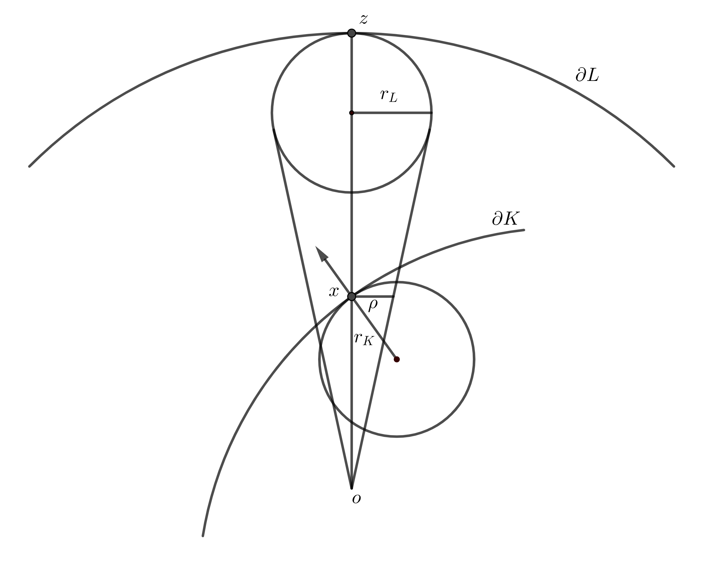
    Figure 1: Case 2a).

  • Now we treat the general case, when $z\in\partial L$ is not necessarily parallel to $N_{L}(z)$. We reduce this case to the previous case. As $x\in\text{int}(L)$, the line segment

    $$[z_{0},z]=\{\lambda x:\lambda\geq 0\}\cap B_{2}^{n}(z-r_{L}N_{L}(z),r_{L})$$

    is in the interior of $B_{2}^{n}(z-r_{L}N_{L}(z),r_{L})$. Let $w$ be the midpoint of $[z_{0},z]$ and let $\alpha={\rm dist}(w,\partial(B_{2}^{n}(z-r_{L}N_{L}(z),r_{L})))$ be the distance from $w$ to the boundary of $B_{2}^{n}(z-r_{L}N_{L}(z),r_{L}))$. Then

    $$B_{2}^{n}(w,\alpha/2)\subset B_{2}^{n}(z-r_{L}N_{L}(z),r_{L}).$$

    Now we consider the cone that is the convex hull of the origin $o$ and the ball $B^{n}_{2}(w,\alpha/2)$. We then proceed as above, replacing $z$ by $w+\alpha/2\frac{x}{||x||}$, also noting that $||w+\alpha/2\frac{x}{||x||}||\leq||z||$.

The proof that $K\cap L$ and $K\cup L$ admit an outer rolling ball is similar to the above, though slightly more technical.

4.2 Special Cases

The $L_{p}$-Steiner quermassintegrals generalize the known quermassintegrals, the dual mixed volumes and the mixed $L_{p}$ affine surface areas. Indeed, (i) If $p=0$ and $K$ is $C^{2}_{+}$,

$$\mathcal{V}^{0}_{k}(K)=n\binom{n}{k}\,W_{k}(K).$$ (27)

Then (27) can be deduced immediately as follows. From (15) we get that

$$as_{0}(K+tB^{n}_{2})=\sum_{k=0}^{\infty}\mathcal{V}^{0}_{k}(K)\,t^{k}.$$ (28)

On the other hand, by the classical Steiner formula,

$$as_{0}(K+tB^{n}_{2})=n\,{\rm vol}_{n}\left(K+tB^{n}_{2}\right)=\sum_{k=0}^{n}\binom{n}{k}\,\mathcal{W}_{k}(K)\,t^{k}.$$ (29)

Comparing (28) and (29), we see that $\mathcal{V}^{0}_{k}(K)=0$ for all $k>n$ and for $0\leq k\leq n$ (27) follows immediately. (ii) If $p=\pm\infty$ and $K$ is $C^{2}_{+}$, we get from the definition that

$$\mathcal{V}^{\pm\infty}_{k}(K)=\binom{-n}{k}\widetilde{W}_{-k}(K^{\circ})=(-1)^{k}\binom{n+k-1}{k}\widetilde{W}_{-k}(K^{\circ}),$$

where $\widetilde{W}_{k}(K)$ are the dual quermassintegrals, [17]. (iii) The $L_{p}$-Steiner quermassintegrals generalize the known mixed $L_{p}$ affine surface areas [18, 39]. We recall that for all $p\neq-n$ and all real $s$, the $s$-th mixed $L_{p}$ affine surface area of $K$ is defined as

$$as_{p,\,s}(K)=\int\limits_{\partial K}H_{n-1}(x)^{\frac{s+p}{n+p}}\langle x,N(x)\rangle^{(1-p)\frac{n-s}{n+p}}d\mathcal{H}^{n-1}(x).$$

Then we get for $k=l(n-1)$, $l\in\mathbb{N}$ and $p=1$,

$$\mathcal{V}_{l(n-1)}^{1}(K)=\mathcal{W}_{l(n-1),\,l(n-1)}(K)=\binom{\frac{n}{n+1}}{l}as_{1,l(n+1)}(K).$$

Similarly, for $m=0$,

$$\mathcal{W}^{p}_{0,\,k}(K)=\int\limits_{\partial K}\langle x,N(x)\rangle^{-k+\frac{n(1-p)}{n+p}}H_{n-1}^{\frac{p}{n+p}}\,d\mathcal{H}^{n-1}(x)=as_{p+\frac{k}{n}(n+p),\,-k}(K).$$ (30)

Note that the term $\mathcal{W}^{p}_{0,\,k}(K)$, which corresponds to the last summand in $\mathcal{V}^{p}_{k}(K)$, is finite and positive for all $k$ and $p$ such that $\frac{p}{n+p}\geq 0$. However, for $p<0$, it may become infinite (see Example 4.2). When, in addition, $p=0$ and $k=1$, $\mathcal{W}^{0}_{0,\,1}(K)$ is the surface area ${\rm vol}_{n-1}(\partial K)$ of $K$. (iv) For the Euclidean unit ball $B^{n}_{2}$ and all parameters $p\neq-n$ we get that

$$\mathcal{V}^{p}_{k}(B^{n}_{2}) = \sum\limits_{m=0}^{k}\binom{\frac{n(1-p)}{n+p}}{k-m}\mathcal{W}^{p}_{m,\,k}(B^{n}_{2})$$ (31)

$$= {\rm vol}_{n-1}(\partial B^{n}_{2})\,\sum\limits_{m=0}^{k}\binom{\frac{n(1-p)}{n+p}}{k-m}\sum_{\begin{subarray}{c}i_{1},\dots,i_{n-1}\geq 0\\ i_{1}+2i_{2}+\dots+(n-1)i_{n-1}=m\end{subarray}}c(n,p,i(m))\prod\limits_{j=1}^{n-1}{n-1\choose j}^{i_{j}}.$$

We define

$$C(n,p,k)=\sum\limits_{m=0}^{k}\binom{\frac{n(1-p)}{n+p}}{k-m}\sum_{\begin{subarray}{c}i_{1},\dots,i_{n-1}\geq 0\\ i_{1}+2i_{2}+\dots+(n-1)i_{n-1}=m\end{subarray}}c(n,p,i(m))\prod\limits_{j=1}^{n-1}{n-1\choose j}^{i_{j}}.$$ (32)

Then,

$$\mathcal{V}^{p}_{k}(B^{n}_{2})=C(n,p,k)\,{\rm vol}_{n-1}(\partial B^{n}_{2}).$$ (33)

In particular,

$$C(n,1,k)=\sum_{\begin{subarray}{c}i_{1},\dots,i_{n-1}\geq 0\\ i_{1}+2i_{2}+\dots+(n-1)i_{n-1}=k\end{subarray}}c(n,1,i(k))\prod\limits_{j=1}^{n-1}{n-1\choose j}^{i_{j}}$$ (34)

and

$$\mathcal{W}_{k,\,k}(B^{n}_{2})={\rm vol}_{n-1}(\partial B^{n}_{2})\,C(n,1,k).$$ (35)

(v) Polytopes $P$ are not in $\mathcal{C}_{p}$ but we would like to note that for polytopes the $L_{p}$-Steiner quermassintegrals exhibit similar properties as the $L_{p}$ affine surface areas. By (30),

$$\mathcal{W}_{0,\,k}^{0}(P)=\int\limits_{\partial P}\langle x,N(x)\rangle^{-k+1}\,d\mathcal{H}^{n-1}(x)=as_{k,\,-k}(P),$$

and by definition,

$$\mathcal{V}^{0}_{k}(P)=\binom{1}{k}\,\mathcal{W}_{0,\,k}^{0}(P)=\left\{\begin{aligned} &n\,{\rm vol}_{n}(P)\quad&\text{ if }\,k=0\\ &{\rm vol}_{n-1}(\partial P)\quad&\text{ if }\,k=1\\ &0\quad&\text{ if }\,\,\,k\geq 2.\end{aligned}\right.$$ (36)

For $p\neq 0$, we get for all $k\geq 0$,

$$\mathcal{V}^{p}_{k}(P)=0\,\,\text{ if }\,\,0<p\leq\infty\,\text{ and }\,-\infty\leq p<-n.$$ (37)

4.3 The expressions $C(n,p,k)$

The $L_{p}$ affine surface area is homogeneous of degree $n\frac{n-p}{n+p}$, i.e.,

$$as_{p}(tK)=t^{n\frac{n-p}{n+p}}as_{p}(K).$$ (38)

Hence

$$as_{p}((1+t)B^{n}_{2})=(1+t)^{n\frac{n-p}{n+p}}{\rm vol}_{n-1}(\partial B^{n}_{2})={\rm vol}_{n-1}(\partial B^{n}_{2})\sum_{k=0}^{\infty}{n\frac{n-p}{n+p}\choose k}\ t^{k}.$$ (39)

Observe that for $p=n$, $as_{n}((1+t)B^{n}_{2})={\rm vol}_{n-1}(\partial B^{n}_{2})$ and that on the right hand side of (39) ${0\choose k}=0$ for all $k$, except for $k=0$, when ${0\choose 0}=1$. In particular, this means that

$$C(n,n,k)=\left\{\begin{aligned} &1\quad&\text{ if }\ k=0,\\ &0\quad&\text{ if }\,k\geq 1.\end{aligned}\right.$$

For $p\neq n,-n$, applying (15) when $K$ is the Euclidean unit ball $B^{n}_{2}$, we get

$$as_{p}(B^{n}_{2}+tB^{n}_{2})=\sum_{k=0}^{\infty}\mathcal{V}_{k}^{p}(B^{n}_{2})\,t^{k}.$$

Therefore,

$$\mathcal{V}_{k}^{p}(B^{n}_{2})={\rm vol}_{n-1}(\partial B^{n}_{2}){n\frac{n-p}{n+p}\choose k}$$

which implies that

$$C(n,p,k)={n\frac{n-p}{n+p}\choose k}.$$ (40)

This observation results in the following combinatorial formula.

Corollary 4.3

Let $p\in\mathbb{R}$, $p\neq-n$. Then

$${n\frac{n-p}{n+p}\choose k}=\sum\limits_{m=0}^{k}\binom{\frac{n(1-p)}{n+p}}{k-m}\sum_{\begin{subarray}{c}i_{1},\dots,i_{n-1}\geq 0\\ i_{1}+2i_{2}+\dots+(n-1)i_{n-1}=m\end{subarray}}c(n,p,i(m))\prod\limits_{j=1}^{n-1}{n-1\choose j}^{i_{j}}.$$

We summarize some consequences for the Euclidean ball in the next corollary.

Corollary 4.4

$$(i)\hskip 11.38109pt\mathcal{V}^{0}_{k}(B^{n}_{2})={n\choose k}{\rm vol}_{n-1}(\partial B^{n}_{2})=\left\{\begin{aligned} &{n\choose k}{\rm vol}_{n-1}(\partial B^{n}_{2})\quad&\text{ if }\ 0\leq k\leq n,\\ &0\quad&\text{ if }\,k\geq n+1.\end{aligned}\right.$$

$$(ii)\hskip 11.38109pt\mathcal{V}^{n}_{k}(B^{n}_{2})=C(n,n,k)\,{\rm vol}_{n-1}(\partial B^{n}_{2})=\left\{\begin{aligned} &{\rm vol}_{n-1}(\partial B^{n}_{2})\quad&\text{ if }\ k=0,\\ &0\quad&\text{ if }\,k\geq 1.\end{aligned}\right.$$

$$\hskip-142.26378pt(iii)\hskip 11.38109pt\mathcal{V}_{k}^{p}(B^{n}_{2})={\rm vol}_{n-1}(\partial B^{n}_{2}){n\frac{n-p}{n+p}\choose k}.$$

We now analyze the expressions $C(n,p,k)$ further. This is also needed to determine continuity issues of $L_{p}$-Steiner quermassintegrals in Section 5.3. We start with the case $p=1$.

Proposition 4.5

The following holds for all $n\geq 2$:

• $C(n,1,k)>0$ for $k\leq n-1$;

• $(-1)^{k-n+1}C(n,1,k)>0$ for $k\geq n$.

Proof  

• Denote $\alpha=n\frac{n-1}{n+1}$. Using (40),

  $$C(n,1,k)=\binom{\alpha}{k}=\frac{\alpha(\alpha-1)(\alpha-2)\cdots(\alpha-k+1)}{k(k-1)\cdots 1}.$$ (41)

  It is clear that the denominator is positive. We show that the numerator is also positive when $k\leq n-1$. Note that $\alpha-j=n-2+\frac{2}{n+1}-j$ for $1\leq j\leq k-1$. Then $\alpha-j>0$ when $j\leq n-2$. Since $k\leq n-1$, $j$ can change in the interval $1\leq j\leq n-2$ which implies that $C(n,1,k)>0.$

• The numerator of (41) consists of $k-1$ factors $\alpha-j$ each of which is positive when $j\leq n-2$ and negative when $j\geq n-1.$ If $k\geq n$, the first $n-2$ terms of (41) are positive, and the remaining $k-n+1$ terms are negative which implies the statement.

Now we address the general case.

Proposition 4.6

The following holds for all $n\geq 2$:

• If $p<-n$, then $(-1)^{k}C(n,p,k)>0$ for $k\in\mathbb{N}$;

• If $-n<p<n-2+\frac{2}{n+1}$, then $C(n,p,k)>0$ for all $k\leq\lfloor n-2p+\frac{2p^{2}}{n+p}\rfloor+1$ and $(-1)^{k-(\lfloor n-2p+\frac{2p^{2}}{n+p}\rfloor+1)}C(n,p,k)~{}>~{}0$ for $k>\lfloor n-2p+\frac{2p^{2}}{n+p}\rfloor+1$;

• If $n-2+\frac{2}{n+1}\leq p<n$, then $(-1)^{k-1}C(n,p,k)>0$ for $k\in\mathbb{N}$;

• If $p=n$, then $C(n,p,0)=1$ and $C(n,p,k)=0$ for $k\in\mathbb{N}$;

• If $p>n$, then $(-1)^{k}C(n,p,k)>0$ for $k\in\mathbb{N}$.

Proof   Denote $\alpha=n\frac{n-p}{n+p}$. By (40),

$$C(n,p,k)=\binom{\alpha}{k}=\frac{\alpha(\alpha-1)(\alpha-2)\cdots(\alpha-k+1)}{k(k-1)\cdots 1}.$$ (42)

• Since denominator of (42) is positive, numerator of (42) determines the sign of $C(n,p,k)$. If $p<-n$, then $\alpha<0$ which implies that $\alpha-j<0$ for all $1\leq j\leq k-1$. As there are $k$ negative terms in the numerator, we get the result.

• Here $\alpha-j>0$ when $j\leq\lfloor n-2p+\frac{2p^{2}}{n+p}\rfloor$, and $\alpha-j<0$ otherwise. Since $1\leq j\leq k-1$, if $k\leq\lfloor n-2p+\frac{2p^{2}}{n+p}\rfloor+1$, then $\alpha-j>0$ which yields that $C(n,p,k)>0$. If $k>\lfloor n-2p+\frac{2p^{2}}{n+p}\rfloor+1$, then the first $\lfloor n-2p+\frac{2p^{2}}{n+p}\rfloor$ terms $\alpha-j$ are positive and the remaining $k-(\lfloor n-2p+\frac{2p^{2}}{n+p}\rfloor+1)$ terms are negative which implies the result.

• If $p=n$, then $\alpha=0$, $C(n,p,0)=\binom{0}{0}=1$ and $C(n,p,k)=\binom{0}{k}=0$ for $k\in\mathbb{N}$.

The proof of (iii) and (v) is similar to proof of (i). Remark In the special case when $p=\frac{n(n-l)}{n+l}$, $l\in\mathbb{N}$, $\frac{n(n-p)}{n+p}$ is an integer. This simplifies the binomial coefficients $\binom{\frac{n(n-p)}{n+p}}{k}$ that appear in (23). Thus, the coefficients $C(n,p,k)>0$ for $k\leq l$ and $C(n,p,k)=0$ for $k>l$.

5 Properties of the $L_{p}$-Steiner quermassintegrals

5.1 Homogeneity and Invariance

Theorem 5.1

Let $K$ be a convex body in $\mathcal{C}^{n}$ and let $p\in\mathbb{R}$ be such that $p\geq 0$ or $p<-n$. Then for all $k\in\mathbb{N}$, we have

• $\mathcal{W}^{p}_{m,\,k}(K)$ and $\mathcal{V}^{p}_{k}(K)$ are homogeneous of degree $n\frac{n-p}{n+p}-k$.

• $\mathcal{W}^{p}_{m,\,k}(K)$ and $\mathcal{V}^{p}_{k}(K)$ are invariant under rotations and reflections.

Remark Property (i) of Theorem 5.1 implies that for the Euclidean ball with radius $r$,

$$\mathcal{V}^{p}_{k}(rB^{n}_{2})=r^{n\frac{n-p}{n+p}-k}\,\mathcal{V}^{p}_{k}(B^{n}_{2})=r^{n\frac{n-p}{n+p}-k}\,{\rm vol}_{n-1}(\partial B^{n}_{2})\,C(n,p,k).$$ (43)

The following corollary, for the case $p=1$, immediately follows from Theorem 5.1. In addition to rotation- and reflection-invariance, we also have invariance under translations.

Corollary 5.2

Let $K$ be a convex body in $\mathcal{C}^{n}$. Then for all $k\in\mathbb{N}$, $\mathcal{V}^{1}_{k}=\mathcal{W}_{k,\,k}$ are invariant under rigid motions and homogeneous of degree $n\frac{n-1}{n+1}-k$.

5.1.1 Proof of Theorem 5.1

To show Theorem  5.1, we need the following facts (see, e.g., [33]).

Proposition 5.3

Let $g:\partial K\rightarrow\mathbb{R}$ be an integrable function, and $T:\mathbb{R}^{n}\rightarrow\mathbb{R}^{n}$ be an invertible, linear map. Then

$$\int_{\partial K}g(x)\,d\mathcal{H}^{n-1}(x)=|\det(T)|^{-1}\,\int_{\partial T(K)}\|T^{-1t}(N_{K}(T^{-1}(y)))\|^{-1}g(T^{-1}(y))\,d\mathcal{H}^{n-1}(x)$$

and

$$\langle T^{-1}(y,)N_{K}(T^{-1}y)\rangle=\langle y,N_{T(K)}(y)\rangle\,\|T^{-1t}(N_{K}(T^{-1}(y)))\|$$

for all $y\in\partial T(K)$.

We apply Proposition 5.3 to $\mathcal{W}^{p}_{m,\,k}(K)$ and get

$$\mathcal{W}^{p}_{m,\,k}(K)=$$

$$|\det(T)|^{-1}\,\int\limits_{\partial T(K)}\|T^{-1t}(N_{K}(T^{-1}(y)))\|^{m-k-1+\frac{n(1-p)}{n+p}}\langle y,N_{T(K)}(y)\rangle^{m-k+\frac{n(1-p)}{n+p}}H_{n-1}^{\frac{p}{n+p}}(T^{-1}(y))$$

$$\sum_{\begin{subarray}{c}i_{1},\dots,i_{n-1}\geq 0\\ i_{1}+2i_{2}+\dots+(n-1)i_{n-1}=m\end{subarray}}c(n,p,i(m))\prod\limits_{j=1}^{n-1}{n-1\choose j}^{i_{j}}H_{j}^{i_{j}}\left(T^{-1}(y)\right)\,d\mathcal{H}^{n-1}(y).$$ (44)

(i) Let $a\in\mathbb{R}$. We apply (5.1.1) to $T=a\,Id$. We also use that for $y\in\partial(aK)$,

$$H_{j}(y)=\frac{H_{j}(T^{-1}y)}{a^{j}}.$$

We get

$$\mathcal{W}^{p}_{m,\,k}(K)=a^{k-n\frac{n-p}{n+p}}\,$$

$$\int\limits_{\partial aK}\langle y,N_{aK}(y)\rangle^{m-k+\frac{n(1-p)}{n+p}}H_{n-1}^{\frac{p}{n+p}}(y)\sum_{\begin{subarray}{c}i_{1},\dots,i_{n-1}\geq 0\\ i_{1}+2i_{2}+\dots+(n-1)i_{n-1}=m\end{subarray}}c(n,p,i(m))\prod\limits_{j=1}^{n-1}{n-1\choose j}^{i_{j}}H_{j}^{i_{j}}\left(y\right)\,d\mathcal{H}^{n-1}(y)$$

$$=a^{k-n\frac{n-p}{n+p}}\,\mathcal{W}^{p}_{m,\,k}(aK).$$

Consequently,

$$\mathcal{V}^{p}_{k}(K)=\sum\limits_{m=0}^{k}\binom{\frac{n(1-p)}{n+p}}{k-m}\mathcal{W}^{p}_{m,\,k}(K)=a^{k-n\frac{n-p}{n+p}}\,\sum\limits_{m=0}^{k}\binom{\frac{n(1-p)}{n+p}}{k-m}\mathcal{W}^{p}_{m,\,k}(aK)=a^{k-n\frac{n-p}{n+p}}\,\mathcal{V}^{p}_{k}(aK).$$

(ii) If $T$ is a rotation or a reflection, then $|\det T|=1$, $\|T^{-1t}(N_{K}(T^{-1}(y)))\|=\|N_{K}(T^{-1}(y))\|=1$ and for all $1\leq j\leq n-1$,

$$\{H_{j}(y):y\in\partial T(K)\}=\{H_{j}\left(x\right):\,x\in\partial K\}.$$

Thus

$$\mathcal{W}^{p}_{m,\,k}(K)=$$

$$\int\limits_{\partial T(K)}\langle y,N_{T(K)}(y)\rangle^{m-k+\frac{n(1-p)}{n+p}}H_{n-1}^{\frac{p}{n+p}}(y)\sum_{\begin{subarray}{c}i_{1},\dots,i_{n-1}\geq 0\\ i_{1}+2i_{2}+\dots+(n-1)i_{n-1}=m\end{subarray}}c(n,p,i(m))\prod\limits_{j=1}^{n-1}{n-1\choose j}^{i_{j}}H_{j}^{i_{j}}\left(y\right)\,d\mathcal{H}^{n-1}(y)$$

$$=\mathcal{W}^{p}_{m,\,k}(T(K)),$$

which implies

$$\mathcal{V}^{p}_{k}(K)=\sum\limits_{m=0}^{k}\binom{\frac{n(1-p)}{n+p}}{k-m}\mathcal{W}^{p}_{m,\,k}(K)=\sum\limits_{m=0}^{k}\binom{\frac{n(1-p)}{n+p}}{k-m}\mathcal{W}^{p}_{m,\,k}(T(K))=\mathcal{V}^{p}_{k}(T(K)).$$

Remarks 1. Under the additional assumption that $K$ is $C^{2}_{+}$, the proof of the homogeneity property is an immediate consequence of the homogeneity of $L_{p}$ affine surface area and (15). Indeed, we have

$$as_{p}(\lambda K+tB^{n}_{2})=as_{p}\left(\lambda\left(K+\frac{t}{\lambda}B^{n}_{2}\right)\right)=\lambda^{n\frac{n-p}{n+p}}as_{p}\left(K+\frac{t}{\lambda}B^{n}_{2}\right)=\sum\limits_{k=0}^{\infty}\mathcal{V}^{p}_{k}(K)\lambda^{n\frac{n-p}{n+p}-k}t^{k}.$$

On the other hand, using (15) directly, we get

$$as_{p}(\lambda K+tB)=\sum\limits_{k=0}^{\infty}\mathcal{V}^{p}_{k}(\lambda K)t^{k}.$$

Therefore,

$$\mathcal{V}^{p}_{k}(\lambda K)=\lambda^{n\frac{n-p}{n+p}-k}\mathcal{V}^{p}_{k}(K).$$

2. We cannot expect that $\mathcal{V}^{p}_{k}(K),\mathcal{W}^{p}_{m,\,k}(K)$ are invariant under general linear transformations. For instance, by (5.1.1), and also using (see [33]) that

$$H_{n-1}(x)=\|T^{-1t}(N_{K}(x))\|^{n+1}|\det(T)|^{2}H_{n-1}(T(x))$$

we have

$$\mathcal{V}^{p}_{1}(K) = \frac{n(1-p)}{n+p}\mathcal{W}^{p}_{0,\,1}(K)+\mathcal{W}^{p}_{1,\,1}(K)=\frac{n}{n+p}|\det(T)|^{-\frac{n-p}{n+p}}\,$$

$$\Bigg{(}(1-p)\,\int\limits_{\partial T(K)}\|T^{-1t}(N_{K}(T^{-1}(y)))\|^{-1}\langle y,N_{T(K)}(y)\rangle^{-1+\frac{n(1-p)}{n+p}}H_{n-1}^{\frac{p}{n+p}}(y)\,d\mathcal{H}^{n-1}(y)$$

$$+ (n-1)\int\limits_{\partial T(K)}\langle y,N_{T(K)}(y)\rangle^{\frac{n(1-p)}{n+p}}H_{n-1}^{\frac{p}{n+p}}(y)H_{1}(T^{-1}(y))\,d\mathcal{H}^{n-1}(y)\Bigg{)}$$

In particular, if $n=2$, then $H_{n-1}=H_{1}$ and thus

$$\mathcal{V}^{p}_{1}(K) = \frac{2(1-p)}{2+p}\mathcal{W}^{p}_{0,\,1}(K)+\mathcal{W}^{p}_{1,\,1}(K)=$$

$$\hskip-31.29802pt\frac{2}{2+p}|\det(T)|^{-\frac{2-p}{2+p}}\Bigg{(}(1-p)\,\int\limits_{\partial T(K)}\|T^{-1t}(N_{K}(T^{-1}(y)))\|^{-1}\langle y,N_{T(K)}(y)\rangle^{-1+\frac{2(1-p)}{2+p}}H_{1}^{\frac{2}{2+p}}(y)\,d\mathcal{H}^{1}(y)$$

$$\hskip-31.29802pt+|\det(T)|^{2}\int\limits_{\partial T(K)}\|T^{-1t}(N_{K}(T^{-1}(y)))\|^{3}\langle y,N_{T(K)}(y)\rangle^{\frac{2(1-p)}{2+p}}H_{1}^{\frac{2(p+1)}{2+p}}(y)\,d\mathcal{H}^{1}(y)\Bigg{)},$$

while

$$\mathcal{V}^{p}_{1}(T(K))=\frac{2(1-p)}{2+p}\mathcal{W}^{p}_{0,\,1}(T(K))+\mathcal{W}^{p}_{1,\,1}(T(K))=$$

$$\hskip-28.45274pt\frac{2}{2+p}\Bigg{(}(1-p)\int\limits_{\partial T(K)}\langle y,N(y)\rangle^{-1+\frac{2(1-p)}{2+p}}H_{1}^{\frac{2}{2+p}}(y)\,d\mathcal{H}^{1}(y)+\int\limits_{\partial T(K)}\langle y,N(y)\rangle^{\frac{2(1-p)}{2+p}}H_{1}^{\frac{2(p+1)}{2+p}}(y)\,d\mathcal{H}^{1}(y)\Bigg{)}.$$

That is, unless $T$ is an isometry, we cannot expect to have invariance.

5.2 Valuation property

For $p=1$, we have the following

Theorem 5.4

For all $k\in\mathbb{N}$, $\mathcal{W}_{k,\,k}$ are valuations on the set $\mathcal{C}^{n}$.

More generally, we obtain

Theorem 5.5

Let $p\in\mathbb{R}$ be such that $p\geq 0$ or $p<-n$. For all $k,m\in\mathbb{N}$, $\mathcal{W}_{m,\,k}^{p}$ and $\mathcal{V}^{p}_{k}$ are valuations on the set $\mathcal{C}^{n}$.

5.2.1 Proof of Theorem 5.4 and Theorem 5.5

We need the following lemma which can be found in e.g. [31].

Lemma 5.6

Let $C$ and $K$ be convex bodies in $\mathbb{R}^{n}$ and suppose that $C\cup K$ is a convex body. Then we have for all $x\in\partial C\cap\partial K$ and for all $\alpha\geq 0$ where the principal curvatures $k_{j}(\partial(C\cup K),x)$, $k_{j}(\partial(C\cap K),x)$, $k_{j}(C,x)$ and $k_{j}(K,x)$ exist for all $1\leq j\leq n-1$,

$$H_{n-1}(\partial(C\cup K),x)^{\frac{1}{n+1}}k_{j}(\partial(K\cup C),x)^{\alpha}=\min\{H_{n-1}(C,x)^{\frac{1}{n+1}}k_{j}(C,x)^{\alpha},H_{n-1}(K,x)^{\frac{1}{n+1}}k_{j}(K,x)^{\alpha}\}$$

and

$$H_{n-1}(\partial(C\cap K),x)^{\frac{1}{n+1}}k_{j}(\partial(K\cap C),x)^{\alpha}=\max\{H_{n-1}(C,x)^{\frac{1}{n+1}}k_{j}(C,x)^{\alpha},H_{n-1}(K,x)^{\frac{1}{n+1}}k_{j}(K,x)^{\alpha}\}.$$

Moreover, for all $1\leq i_{1},\dots,i_{j}\leq n-1$, and for all $\alpha_{1},\alpha_{2},\dots,\alpha_{j}\geq 0$,

$$H_{n-1}(\partial(C\cup K),x)^{\frac{1}{n+1}}\prod_{i=1}^{j}k_{i_{j}}(\partial(K\cup C),x)^{\alpha_{j}}=$$

$$\min\{H_{n-1}(C,x)^{\frac{1}{n+1}}\prod_{i=1}^{j}k_{i_{j}}(C,x)^{\alpha_{j}},H_{n-1}(K,x)^{\frac{1}{n+1}}\prod_{i=1}^{j}k_{i_{j}}(K,x)^{\alpha_{j}}\}$$

and

$$H_{n-1}(\partial(C\cap K),x)^{\frac{1}{n+1}}\prod_{i=1}^{j}k_{i_{j}}(\partial(K\cap C),x)^{\alpha_{j}}=$$

$$\max\{H_{n-1}(C,x)^{\frac{1}{n+1}}\prod_{i=1}^{j}k_{i_{j}}(C,x)^{\alpha_{j}},H_{n-1}(K,x)^{\frac{1}{n+1}}\prod_{i=1}^{j}k_{i_{j}}(K,x)^{\alpha_{j}}\}.$$

Theorem 5.7

Let $p\in\mathbb{R}$ be such that $p\geq 0$ or $p<-n$. For all $1\leq i_{1},\dots,i_{j}\leq n-1$ and $\alpha_{1},\alpha_{2},\dots,\alpha_{j}~{}\geq~{}0$,

$$\int\limits_{\partial K}H_{n-1}^{\frac{1}{n+1}}(x)\ \prod_{i=1}^{j}k_{i_{j}}^{\alpha_{j}}(x)\,d\mathcal{H}^{n-1}(x)$$

are valuations on the set $\mathcal{C}^{n}$.

Proof   Since $C$ and $K$ are in $\mathcal{C}^{n}$, then $C\cap K$ and $C\cup K$ are in $\mathcal{C}^{n}$ by Proposition 4.2. To prove the valuation property, we follow the approach of [31]. Let $C$ and $K$ be convex bodies in $\mathbb{R}^{n}$ such that $C\cup K$ is a convex body. As above, we decompose

$$\partial(C\cup K) = \{\partial C\cap\partial K\}\cup\{\partial C\cap K^{c}\}\cup\{C^{c}\cap\partial K\}$$

$$\partial(C\cap K) = \{\partial C\cap\partial K\}\cup\{\partial C\cap\operatorname{int}(K)\}\cup\{\operatorname{int}(C)\cap\partial K\}$$

$$\partial C = \{\partial C\cap\partial K\}\cup\{\partial C\cap K^{c}\}\cup\{\partial C\cap\operatorname{int}(K)\}$$

$$\partial K = \{\partial C\cap\partial K\}\cup\{\partial K\cap C^{c}\}\cup\{\partial K\cap\operatorname{int}(C)\}.$$

Since all the sets (except possibly $\partial C\cap\partial K$) in the right-hand side of the above decomposition are open subsets of $\partial C$, $\partial K$, $\partial(C\cap K)$ and $\partial(C\cup K)$, the integrals over those sets cancel out. Below we use $d\mathcal{H}^{n-1}_{K}(x)$ to denote the usual surface area measure on $\partial K$ and $k_{j}(K,x)$ to emphasize that this is the principal curvature of $K$ at point $x$. It remains to show

$$\int_{\partial C\cap\partial K}H_{n-1}(\partial(C\cup K),x)^{\frac{1}{n+1}}\prod_{i=1}^{j}k_{i_{j}}(\partial(K\cup C),x)^{\alpha_{j}}d\mathcal{H}^{n-1}_{C\cup K}(x)$$

$$+\int_{\partial C\cap\partial K}H_{n-1}(\partial(C\cap K),x)^{\frac{1}{n+1}}\prod_{i=1}^{j}k_{i_{j}}(\partial(K\cap C),x)^{\alpha_{j}}d\mathcal{H}^{n-1}_{C\cap K}(x)$$

$$=\int_{\partial C\cap\partial K}H_{n-1}(C,x)^{\frac{1}{n+1}}\prod_{i=1}^{j}k_{i_{j}}(C,x)^{\alpha_{j}}d\mathcal{H}^{n-1}_{C}(x)+\int_{\partial C\cap\partial K}H_{n-1}(K,x)^{\frac{1}{n+1}}\prod_{i=1}^{j}k_{i_{j}}(K,x)^{\alpha_{j}}d\mathcal{H}^{n-1}_{K}(x).$$

Please note that $d\mathcal{H}^{n-1}_{C\cup K}=d\mathcal{H}^{n-1}_{C\cap K}$ on $\partial K\cap\partial C$. This holds because both measure are equal to the $(n-1)$-dimensional Hausdorff measure. Therefore, it is left to show

$$\int_{\partial C\cap\partial K}H_{n-1}(\partial(C\cup K),x)^{\frac{1}{n+1}}\prod_{i=1}^{j}k_{i_{j}}(\partial(K\cup C),x)^{\alpha_{j}}d\mathcal{H}^{n-1}_{C\cap K}(x)$$

$$+\int_{\partial C\cap\partial K}H_{n-1}(\partial(C\cap K),x)^{\frac{1}{n+1}}\prod_{i=1}^{j}k_{i_{j}}(\partial(K\cap C),x)^{\alpha_{j}}d\mathcal{H}^{n-1}_{C\cap K}(x)$$

$$=\int_{\partial C\cap\partial K}H_{n-1}(C,x)^{\frac{1}{n+1}}\prod_{i=1}^{j}k_{i_{j}}(C,x)^{\alpha_{j}}d\mathcal{H}^{n-1}_{C}(x)+\int_{\partial C\cap\partial K}H_{n-1}(K,x)^{\frac{1}{n+1}}\prod_{i=1}^{j}k_{i_{j}}(K,x)^{\alpha_{j}}d\mathcal{H}^{n-1}_{K}(x).$$

By Lemma 5.6 this is equivalent to

$$\int_{\partial C\cap\partial K}\min\{H_{n-1}(C,x)^{\frac{1}{n+1}}\prod_{i=1}^{j}k_{i_{j}}(C,x)^{\alpha_{j}},H_{n-1}(K,x)^{\frac{1}{n+1}}\prod_{i=1}^{j}k_{i_{j}}(K,x)^{\alpha_{j}}\}d\mathcal{H}^{n-1}_{C\cap K}(x)$$

$$+\int_{\partial C\cap\partial K}\max\{H_{n-1}(C,x)^{\frac{1}{n+1}}\prod_{i=1}^{j}k_{i_{j}}(C,x)^{\alpha_{j}},H_{n-1}(K,x)^{\frac{1}{n+1}}\prod_{i=1}^{j}k_{i_{j}}(K,x)^{\alpha_{j}}\}d\mathcal{H}^{n-1}_{C\cap K}(x)$$

$$=\int_{\partial C\cap\partial K}H_{n-1}(C,x)^{\frac{1}{n+1}}\prod_{i=1}^{j}k_{i_{j}}(C,x)^{\alpha_{j}}d\mathcal{H}^{n-1}_{C}(x)+\int_{\partial C\cap\partial K}H_{n-1}(K,x)^{\frac{1}{n+1}}\prod_{i=1}^{j}k_{i_{j}}(K,x)^{\alpha_{j}}d\mathcal{H}^{n-1}_{K}(x).$$

This holds since for any real numbers $a$ and $b$, we have

$$a+b=\min\{a,b\}+\max\{a,b\}.$$

We note that in the setting of Lemma 5.6, $N_{K}(x)=N_{C}(x)=N_{C\cap K}(x)=N_{C\cup K}(x)$. Using this observation together with Lemma 5.6 and the decomposition in the proof of Theorem 5.7, we get the following generalization.

Theorem 5.8

Let $p\in\mathbb{R}$ be such that $p\geq 0$ or $p<-n$. For all $1\leq i_{1},\dots,i_{j}\leq n-1$ and $\alpha_{1},\alpha_{2},\dots,\alpha_{j}~{}\geq~{}0$,

$$\int\limits_{\partial K}\langle x,N(x)\rangle^{m-k+\frac{n(1-p)}{n+p}}H_{n-1}^{\frac{p}{n+p}}(x)\ \prod_{i=1}^{j}k_{i_{j}}^{\alpha_{j}}(x)\,d\mathcal{H}^{n-1}(x)$$

are valuations on the set $\mathcal{C}^{n}$.

Proof of Theorem 5.4   The result follows immediately from Theorem 5.7 as

$$\mathcal{W}_{k,\,k}(K)=\int\limits_{\partial K}H_{n-1}^{\frac{1}{n+1}}(x)\sum_{\begin{subarray}{c}i_{1},\dots,i_{n-1}\geq 0\\ i_{1}+2i_{2}+\dots+(n-1)i_{n-1}=k\end{subarray}}c(n,1,i(k))\prod\limits_{j=1}^{n-1}{n-1\choose j}^{i_{j}}H_{j}^{i_{j}}\left(x\right)\,d\mathcal{H}^{n-1}(x)$$

is a sum (up to constants) of integrals of the form

$$\int\limits_{\partial K}H_{n-1}^{\frac{1}{n+1}}(x)\ \prod_{i=1}^{j}k_{i_{j}}^{\alpha_{j}}(x)\,d\mathcal{H}^{n-1}(x)$$

and as the sum of valuations, it is again a valuation.

Proof of Theorem 5.5 The result follows immediately from Theorem 5.8 and the fact that the linear combination of valuations is again a valuation.

Remark When $j=n-1$, Theorem 5.7 states that for any $\alpha_{1},\dots,\alpha_{n-1}\geq 0$

$$\int\limits_{\partial K}H^{\frac{1}{n+1}}_{n-1}(x)\prod_{i=1}^{n-1}k_{i}^{\alpha_{i}}(x)\,d\mathcal{H}^{n-1}(x)$$

is a valuation on the set $\mathcal{C}^{n}$. In particular, when $\alpha_{1}=\dots=\alpha_{n-1}=\frac{s}{n+1}$ for any $s>0$, then

$$\int\limits_{\partial K}H^{\frac{1}{n+1}}_{n-1}(x)\left(\prod_{i=1}^{n-1}k_{i}(x)\right)^{\frac{s}{n+1}}\,d\mathcal{H}^{n-1}(x)=\int\limits_{\partial K}H^{\frac{s+1}{n+1}}_{n-1}(x)\,d\mathcal{H}^{n-1}(x)=as_{1,s}(K)$$

and Theorem 5.7 implies that mixed affine surface areas $as_{1,s}$ are valuations. It seems that this fact was not known before.

5.3 Continuity

For convex bodies $K$ and $L$, their Hausdorff distance is

$$d_{H}(K,L)=\min\{\varepsilon:K\subset L+\varepsilon B_{2}^{n},L\subset K+\varepsilon B_{2}^{n}\}.$$ (45)

It was proved by Lutwak [20] (see also [14]) that for $p\geq 1$, $L_{p}$ affine surface area is an upper semi continuous functional with respect to the Hausdorff metric. In fact, it follows from Lutwak’s proof that the same holds for all $0\leq p<1$ (aside from the case $p=0$, which is just volume and hence continuous). For $-n<p\leq 0$, the functional is lower semi continuous as was shown by Ludwig [15]. It was also shown there that the functional defined by (11) is not lower semi continuous when $-n<p\leq 0$, and that it is lower semi continuous for $p<-n$ whereas such a statement is not true in this range for the functional defined by (8).

As $\mathcal{V}_{0}^{p}(K)=\mathcal{W}^{p}_{0,\,0}=as_{p}(K)$, it is natural to ask about the continuity properties for the $L_{p}$-Steiner quermassintegrals $\mathcal{V}_{k}^{p}$ and the $L_{p}$ Steiner coefficients $\mathcal{W}^{p}_{m,\,k}$. Of course, if $p=0$, then $\mathcal{V}_{0}^{0}(K)=n\,{\rm vol}_{n}(K)$, which is continuous. We first consider the cases when the assumption $K\in\mathcal{C}^{n}$ is not needed. This holds for $\mathcal{W}^{p}_{0,\,k}$ (30). As these coincide with the mixed $L_{p}$ affine surface areas $as_{p+\frac{k}{n}(n+p),-k}$, this shows the continuity properties of the latter, which, as far as we know, had not been stated before.

Theorem 5.9

Let $k\geq 0$.

• For $0\leq p\leq\infty$, $\mathcal{W}^{p}_{0,\,k}$ is upper semi continuous on the set $\mathcal{K}^{n}_{o}$ and for $-n<p\leq 0$, lower semi continuous on the set $\mathcal{K}^{n}_{o}$.

• The $as_{p,s}(K)$ are upper semi continuous on the set $\mathcal{K}^{n}_{o}$ when $s<0$ and $p>-s$, and lower semi continuous on the set $\mathcal{K}^{n}_{o}$ if $s<0$ and $-n<p<-s$.

Proof   We prove part (i). Part (ii) follows similarly. We note that if $K_{l}$ converges to $K$ in the Hausdorff metric, then $h_{K_{l}}$ converges to $h_{K}$ uniformly on $S^{n-1}$. Using 30, the proof of (i) then follows from the proof of upper semi continuity of a generalized $L_{p}$ affine surface area given in [14] where we take $f(t)=t^{\frac{p}{n+p}}$ that satisfies the conditions in [14] (since $0<\frac{p}{n+p}<1$). The next corollary follows immediately from this theorem and the previous sections. A characterization of upper semi continuous rigid motion invariant valuations on convex bodies in the plane was given in [13].

Corollary 5.10

Let $p\geq 0$. Then $\mathcal{W}^{p}_{0,\,k}=as_{p+\frac{k}{n}(n+p),-k}$ are upper semi continuous $n\frac{n-p}{n+p}~{}-~{}k$ homogeneous valuations on the set $\mathcal{K}^{n}_{o}$ that are invariant under rotations and reflections.

We will repeatedly use the following example:
For $x\in\mathbb{R}^{n}$, let $\|x\|_{\infty}=\max_{1\leq i\leq n}|x_{i}|$ and let $B^{n}_{\infty}=\{x\in\mathbb{R}^{n}:\|x\|_{\infty}\leq 1\}$. For $l\in\mathbb{N}$, we consider convex bodies $K_{l}$. We describe $K_{l}$ for the first quadrant $\mathbb{R}^{n}_{+}$, and call them $K_{l}^{+}$. The other quadrants are described accordingly. Let $x_{0}=(1-\frac{1}{l},\cdots,1-\frac{1}{l})$ and $B^{n}_{2}\left(x_{0},\frac{1}{l}\right)$ be the Euclidean ball centered at $x_{0}$ with radius $\frac{1}{l}$. We put

$$K_{l}^{+}=\left(1-\frac{1}{l}\right)B^{n}_{\infty}+\frac{1}{l}B^{n}_{2}.$$ (46)

Remark Let $K_{l}$ be as in (46). Then $K_{l}\rightarrow B^{n}_{\infty}$ in the Hausdorff metric and $\mathcal{W}^{p}_{0,\,k}(B^{n}_{\infty})=0$ for $-\infty\leq p<-n$. Moreover,

$$\mathcal{W}^{p}_{0,\,k}(K_{l}) = \int\limits_{\partial K_{l}}H_{n-1}^{\frac{p}{n+p}}\langle x,N(x)\rangle^{-k-n\frac{p-1}{n+p}}d\mathcal{H}^{n-1}(x)$$

$$\geq n^{\frac{1}{2}\left(-k-n\frac{p-1}{n+p}\right)}\,l^{-n\frac{n-p}{n+p}}{\rm vol}_{n-1}\,\,(\partial B^{n}_{2})\rightarrow\infty,$$

as $l\rightarrow\infty$. This shows that $\mathcal{W}^{p}_{0,\,k}$ is not upper semi continuous for $-\infty\leq p<-n$. It is also not lower semi continuous for that $p$-range as is easily seen by taking a sequence of polytopes that converges to the Euclidean unit ball.

While there are continuity properties of the $L_{p}$ Steiner coefficients for $m=0$, we cannot expect that any of the other $L_{p}$ Steiner coefficients or $L_{p}$-Steiner quermassintegrals have continuity properties.

We note that $\mathcal{C}^{n}$ is not closed under the topology generated by the Hausdorff metric. Thus, when addressing continuity issues, we consider convergence in the Hausdorff topology involving bodies for which the $L_{p}$ Steiner coefficients are well-defined but such that these bodies are not necessarily in $\mathcal{C}^{n}$.

Proposition 5.11

Let $k\geq 1$. Then $\mathcal{V}^{1}_{k}=\mathcal{W}_{k,\,k}$ are neither lower semi continuous nor upper semi continuous.

Proof   It is clear that $\mathcal{W}_{k,\,k}$ is not continuous with respect to the Hausdorff metric: take a sequence of polytopes that approximates the Euclidean ball.

Let $K_{l}$ be as in (46). Then $K_{l}\rightarrow B^{n}_{\infty}$ in the Hausdorff metric and $\mathcal{W}_{k,\,k}(B^{n}_{\infty})=0$. Moreover, even though $K_{l}$ is not in $\mathcal{C}_{p}$, the coefficients $\mathcal{W}_{k,\,k}(K_{l})$ are well-defined. Indeed, using (35),

$$\mathcal{W}_{k,\,k}(K_{l}) = \int\limits_{\partial K_{l}}H_{n-1}^{\frac{1}{n+1}}\sum_{\begin{subarray}{c}i_{1},\dots,i_{n-1}\geq 0\\ i_{1}+2i_{2}+\dots+(n-1)i_{n-1}=k\end{subarray}}c(n,1,i(k))\prod\limits_{j=1}^{n-1}{n-1\choose j}^{i_{j}}H_{j}^{i_{j}}\left(x\right)\,d\mathcal{H}^{n-1}(x)$$ (47)

$$= \int\limits_{\partial B^{n}_{2}\left(0,\frac{1}{l}\right)}H_{n-1}^{\frac{1}{n+1}}\sum_{\begin{subarray}{c}i_{1},\dots,i_{n-1}\geq 0\\ i_{1}+2i_{2}+\dots+(n-1)i_{n-1}=k\end{subarray}}c(n,1,i(k))\prod\limits_{j=1}^{n-1}{n-1\choose j}^{i_{j}}H_{j}^{i_{j}}\left(x\right)\,d\mathcal{H}^{n-1}(x)$$

$$= \mathcal{W}_{k,\,k}\left(B^{n}_{2}\left(0,\frac{1}{l}\right)\right)$$

$$= l^{k-n\frac{n-1}{n+1}}{\rm vol}_{n-1}\,\,(\partial B^{n}_{2})\,C(n,1,k).$$

Let first $k\geq n$. If $k-n+1$ is even, then we have by Proposition 4.5 that $C(n,1,k)>0$. Therefore, as $k-n\frac{n-1}{n+1}>0$,

$$\mathcal{W}_{k,\,k}(K_{l})=l^{k-n\frac{n-1}{n+1}}{\rm vol}_{n-1}\,\,(\partial B^{n}_{2})\,C(n,1,k)\to\infty,$$

as $l\to\infty$, but $\mathcal{W}_{k,\,k}(B^{n}_{\infty})=0$. Thus $\mathcal{W}_{k,\,k}$ is not upper semi continuous in this case. $\mathcal{W}_{k,\,k}$ is also not lower semi continuous. We take a sequence $P_{l}$ of polytopes that converges to $B^{n}_{2}$ in the Hausdorff metric. Then $\mathcal{W}_{k,\,k}(P_{l})=0$ for all $l$ but $\mathcal{W}_{k,\,k}(B^{n}_{2})>0$.

Let now $k\geq n$ be such that $k-n+1$ is odd. Then $C(n,1,k)<0$ by Proposition 4.5 and thus by (31), $\mathcal{W}_{k,\,k}(B^{n}_{2})={\rm vol}_{n-1}(\partial B^{n}_{2})\,C(n,1,k)<0$. As $\mathcal{W}_{k,\,k}(P_{l})=0$ for all $l$, where $P_{l}$ is a sequence of polytopes that converges to $B^{n}_{2}$ in the Hausdorff metric, this shows that $\mathcal{W}_{k,\,k}$ is not lower semi continuous in this case. $\mathcal{W}_{k,\,k}$ is also not upper semi continuous. Indeed, $K_{l}\to B^{n}_{\infty}$ as $l\to\infty$ in the Hausdorff metric and $\mathcal{W}_{k,\,k}(B^{n}_{\infty})=0$. But

$$\mathcal{W}_{k,\,k}(K_{l})=l^{k-n\frac{n-1}{n+1}}{\rm vol}_{n-1}\,\,(\partial B^{n}_{2})\,C(n,1,k)\to-\infty.$$

This settles negatively the semi continuity of $\mathcal{W}_{k,\,k}$ for all $n\geq 2$ and all $k\geq n$. Let now $k\leq n-1$. By (31), we have that $\mathcal{W}_{k,\,k}(B^{n}_{2})={\rm vol}_{n-1}(\partial B^{n}_{2})\,C(n,1,k)>0$. As $\mathcal{W}_{k,\,k}(P)=0$ for every polytope $P$, and as by Proposition 4.5, $C(n,1,k)>0$ for all $n\geq 2$, this shows that $\mathcal{W}_{k,\,k}$ is not lower semi continuous in this $k$-range. Moreover, by Proposition 4.5, for every $n\geq 2$, $C(n,1,n-1)>0$. Therefore, for all $n\geq 2$

$$\mathcal{W}_{n-1,\,n-1}(K_{l})=l^{\frac{n-1}{n+1}}\,{\rm vol}_{n-1}\,\,(\partial B^{n}_{2})\,C(n,1,n-1)\rightarrow\infty,$$

as $l\rightarrow\infty$ and thus $\mathcal{W}_{n-1,\,n-1}$ is also not upper semi continuous, which settles negatively the semi continuity of $\mathcal{W}_{k,\,k}$ for all $n\geq 2$ and all $k\geq n-1$. In particular, the case $n=2$ is settled for all $k$. To settle upper semi continuity for all dimensions and all $k<n-1$ requires further examples.

For instance, for $n=3$, only upper semi continuity for $k=1$ is not yet settled. To resolve this, we consider

$$\mathcal{W}_{1,\,1}(K)=\frac{3}{2}\int_{\partial K}H_{2}(x)^{\frac{1}{4}}\ H_{1}(x)\ d\mathcal{H}^{2}(x).$$

We place the body $K_{l}$ in the $xz$-plane and we let $Z_{l}\subset\mathbb{R}^{3}$ be the body of revolution obtained by rotating $K_{l}$ about the $z$-axis. Let $x\in\partial Z_{l}$. Then the maximal principle curvature $\kappa_{1}(x)=l$ and the minimal principle curvature $\kappa_{2}(x)\geq 1$. Therefore,

$$H_{2}(x)^{\frac{1}{4}}\geq l^{\frac{1}{4}}\hskip 8.53581pt\text{and}\hskip 8.53581ptH_{1}(x)\geq\frac{1}{2}\left(l+1\right)$$

and consequently

$$\mathcal{W}_{1,\,1}(Z_{l})\geq\frac{3}{4}l^{\frac{1}{4}}\left(l+1\right)\int_{\partial Z_{l}}d\mathcal{H}^{2}(x)\geq 3\pi l^{\frac{1}{4}}\left(l+1\right)\frac{1-\frac{1}{l}}{l}.$$

Thus $\mathcal{W}_{1,\,1}(Z_{l})\to\infty$, as $l\to\infty$, but $Z_{l}$ converges in the Hausdorff metric to the cylinder $Z$ of height $2$ and a $2$-dimensional Euclidean unit ball as base and $\mathcal{W}_{1,\,1}(Z)=0$. Thus $\mathcal{W}_{1,\,1}$ is not upper semi continuous and this settles $n=3$ for all $k$.

Modifications of these examples show that $\mathcal{W}_{k,\,k}$ is not upper semi continuous for all $n\geq 4$ and all $1\leq k<n-1$.

Now we treat general parameters $p$ such that $\frac{p}{n+p}\geq 0$. $\mathcal{V}_{0}^{0}(K)=n\,{\rm vol}_{n}(K)$ and $\mathcal{V}_{1}^{0}(K)=c(n){\rm vol}_{n-1}(\partial K)$, where $c(n)$ is a constant depending only on $n$. Thus, $\mathcal{V}_{0}^{0}$ and $\mathcal{V}_{1}^{0}$ are continuous. Moreover, $\mathcal{V}_{0}^{p}(K)=as_{p}(K)$ which, as noted above, is upper semi continuous when $p\geq 0$ and lower semi continuous for $-n<p\leq 0$. In general however, we do not have any continuity property.

Proposition 5.12

Let $-\infty<p<-n$ or $0\leq p<\infty$, and let $k\geq 1$. Let $K$ be such that $\mathcal{V}_{k}^{p}$ are well-defined. Then $\mathcal{V}_{k}^{p}$ are in general neither lower semi continuous nor upper semi continuous.

Proof   If $p=0$ and $k\geq 2$, then by (36), $\mathcal{V}_{k}^{0}(P)=0$ for every polytope $P$ and by Corollary 4.4, $\mathcal{V}^{0}_{k}(B^{n}_{2})={n\choose k}{\rm vol}_{n-1}(\partial B^{n}_{2})$ for $2\leq k\leq n$. Thus, taking a sequence $P_{l}$ of polytopes that converges to $B^{n}_{2}$, this shows that $\mathcal{V}^{0}_{k}$ is not lower semi continuous for $2\leq k\leq n$.
If $p\neq 0$, then by (37), $\mathcal{V}_{k}^{p}(P)=0$ for every polytope $P$ and if $p<-n$ or $p>n$ then by (33) and Proposition 4.6,

$$\mathcal{V}^{p}_{k}(B^{n}_{2})=C(n,p,k)\,{\rm vol}_{n-1}(\partial B^{n}_{2})\left\{\begin{aligned} &<0\quad&\text{ if }\,k\,&\text{ is odd }\\ &>0\quad&\text{ if }\,k\,&\text{ is even }.\end{aligned}\right.$$

Taking a sequence $P_{l}$ of polytopes that converges to $B^{n}_{2}$, shows that for $-\infty\leq p<-n$ or $n<p\leq\infty$, $\mathcal{V}^{p}_{k}$ is not upper semi continuous when $k$ is odd and not lower semi continuous when $k$ is even. Similarly, absence of upper resp. lower semi continuity can be determined for the other $p$-ranges, using Proposition 4.6.

For the semi continuity issues not yet settled, we will now use the convex bodies $K_{l}$, $l\in\mathbb{N}$ given by (46). To determine $\mathcal{V}^{p}_{k}(K_{l})$, it is enough in this case to consider $B_{l}=\partial K_{l}\cap\mathbb{R}^{n}_{+}\cap\partial B^{n}_{2}(x_{0},\frac{1}{l})$, where $x_{0}=\left(1-\frac{1}{l}\right)(1,1,\cdots,1)$. Note that for $x=x_{0}+\frac{1}{l}\xi\in B_{l}$, $\xi\in S^{n-1}_{+}$, we have

$$\langle x,N(x)\rangle=h_{K_{l}}(\xi)=\left(1-\frac{1}{l}\right)\sum_{i=1}^{n}\xi_{i}+\frac{1}{l}.$$ (48)

Then

$$\mathcal{V}_{k}^{p}(K_{l}) = 2^{n}\sum\limits_{m=0}^{k}\binom{\frac{n(1-p)}{n+p}}{k-m}\int\limits_{S^{n-1}_{+}}h_{K_{l}}^{m-k+\frac{n(1-p)}{n+p}}\,\frac{l^{(n-1)\frac{p}{n+p}+m}}{l^{n-1}}$$

$$\sum_{\begin{subarray}{c}i_{1},\dots,i_{n-1}\geq 0\\ i_{1}+2i_{2}+\dots+(n-1)i_{n-1}=m\end{subarray}}c(n,p,i(m))\prod\limits_{j=1}^{n-1}{n-1\choose j}^{i_{j}}\,d\mathcal{H}^{n-1}$$

$$= 2^{n}\sum\limits_{m=0}^{k}l^{-\frac{n(n-1)}{n+p}+m}\binom{\frac{n(1-p)}{n+p}}{k-m}\sum_{\begin{subarray}{c}i_{1},\dots,i_{n-1}\geq 0\\ i_{1}+2i_{2}+\dots+(n-1)i_{n-1}=m\end{subarray}}c(n,p,i(m))\prod\limits_{j=1}^{n-1}{n-1\choose j}^{i_{j}}\,$$

$$\int\limits_{S^{n-1}_{+}}\left(\left(1-\frac{1}{l}\right)\sum_{i=1}^{n}\xi_{i}+\frac{1}{l}\right)^{m-k+\frac{n(1-p)}{n+p}}\,d\mathcal{H}^{n-1},$$

where we used (3) and (48) in the first equality. This shows that $\mathcal{V}_{k}^{p}(K_{l})$ are finite. Therefore,

$$\lim_{l\to\infty}\mathcal{V}_{k}^{p}(K_{l}) = 2^{n}\lim_{l\to\infty}\sum\limits_{m=0}^{k}l^{-\frac{n(n-1)}{n+p}+m}\binom{\frac{n(1-p)}{n+p}}{k-m}\sum_{\begin{subarray}{c}i_{1},\dots,i_{n-1}\geq 0\\ i_{1}+2i_{2}+\dots+(n-1)i_{n-1}=m\end{subarray}}c(n,p,i(m))\prod\limits_{j=1}^{n-1}{n-1\choose j}^{i_{j}}$$

$$\lim_{l\to\infty}\int\limits_{S^{n-1}_{+}}\left(\left(1-\frac{1}{l}\right)\sum_{i=1}^{n}\xi_{i}+\frac{1}{l}\right)^{m-k+\frac{n(1-p)}{n+p}}\,d\mathcal{H}^{n-1}.$$

As for $\xi\in S^{n-1}_{+}$, $1\leq\sum_{i=1}^{n}\xi_{i}\leq\sqrt{n}$, the functions under the integral are uniformly in $l$ bounded by an integrable function and by Lebegue’s Dominated Convergence theorem we can interchange integration and limit. Therefore

$$\lim_{l\to\infty}\int\limits_{S^{n-1}_{+}}\left(\left(1-\frac{1}{l}\right)\sum_{i=1}^{n}\xi_{i}+\frac{1}{l}\right)^{m-k+\frac{n(1-p)}{n+p}}\,d\mathcal{H}^{n-1}=$$

$$\int\limits_{S^{n-1}_{+}}\lim_{l\to\infty}\left(\left(1-\frac{1}{l}\right)\sum_{i=1}^{n}\xi_{i}+\frac{1}{l}\right)^{m-k+\frac{n(1-p)}{n+p}}\,d\mathcal{H}^{n-1}=\int\limits_{S^{n-1}_{+}}\left(\sum_{i=1}^{n}\xi_{i}\right)^{m-k+\frac{n(1-p)}{n+p}}\,d\mathcal{H}^{n-1}.$$

Hence

$$\lim_{l\to\infty}\mathcal{V}_{k}^{p}(K_{l}) = 2^{n}\lim_{l\to\infty}\sum\limits_{m=0}^{k}l^{-\frac{n(n-1)}{n+p}+m}\binom{\frac{n(1-p)}{n+p}}{k-m}\sum_{\begin{subarray}{c}i_{1},\dots,i_{n-1}\geq 0\\ i_{1}+2i_{2}+\dots+(n-1)i_{n-1}=m\end{subarray}}c(n,p,i(m))\,\prod\limits_{j=1}^{n-1}{n-1\choose j}^{i_{j}}$$ (49)

$$\int\limits_{S^{n-1}_{+}}\left(\sum_{i=1}^{n}\xi_{i}\right)^{m-k+\frac{n(1-p)}{n+p}}\,d\mathcal{H}^{n-1}.$$

We look now in more detail at the case $p<-n$. In this case, the exponent $-\frac{n(n-1)}{n+p}+m$ of $l$ in (49) is strictly positive. We observe that for $\alpha\in\mathbb{N}\cup\{0\}$

$$\binom{\frac{n(1-p)}{n+p}}{\alpha}\left\{\begin{aligned} &=0\quad&\text{ if }\,\alpha\,&=0\\ &<0\quad&\text{ if }\,\alpha\,&\text{ is odd }\\ &>0\quad&\text{ if }\,\alpha\,&\text{ is even}.\end{aligned}\right.$$

The analysis of the expression

$$F_{m}(p)=\sum\limits_{\begin{subarray}{c}i_{1},\dots,i_{n-1}\geq 0\\ i_{1}+2i_{2}+\dots+(n-1)i_{n-1}=m\end{subarray}}c(n,p,i(m))\,\prod\limits_{j=1}^{n-1}{n-1\choose j}^{i_{j}}$$

is more involved. We have that

$$F_{1}(p)=(n-1)\,\frac{n}{n+p}$$

which is increasing and $F_{1}(p)\leq 0$ on $[-\infty,-n)$.

$$F_{2}(p)=\frac{(n-1)}{2!}\,\frac{n}{n+p}\left((n-1)\frac{n}{n+p}-1\right),$$

which is decreasing and $F_{2}(p)\geq 0$ on $[-\infty,-n)$.

$$F_{3}(p)=\frac{(n-1)}{3!}\,\frac{n}{n+p}\left((n-1)^{2}\left(\frac{n}{n+p}\right)^{2}-3(n-1)\frac{n}{n+p}+2\right),$$

which is increasing and $F_{3}(p)\leq 0$ on $[-\infty,-n)$.

From the analysis of the signs of $\binom{\frac{n(1-p)}{n+p}}{\alpha}$ and the $F_{m}$ we conclude from (49) that

$$\lim_{l\to\infty}\mathcal{V}_{1}^{p}(K_{l})=-\infty$$

and thus $\mathcal{V}_{1}^{p}$ is not lower semi continuous for $p\in[-\infty,-n)$,

$$\lim_{l\to\infty}\mathcal{V}_{2}^{p}(K_{l})=\infty$$

and thus $\mathcal{V}_{2}^{p}$ is not upper semi continuous for $p\in[-\infty,-n)$,

$$\lim_{l\to\infty}\mathcal{V}_{3}^{p}(K_{l})=-\infty$$

and thus $\mathcal{V}_{3}^{p}$ is not lower semi continuous for $p\in[-\infty,-n)$. Starting from $m=4$, the behavior of $F_{m}$ is not monotone anymore on $[-\infty,0)$.

Similarly, for $n<p<n(n-2)$,

$$\lim_{l\to\infty}\mathcal{V}_{\frac{n(n-1)}{n+p}}^{p}(K_{l})=F_{\frac{n(n-1)}{n+p}}(p)\int\limits_{S^{n-1}}\left(\sum_{i=1}^{n}\xi_{i}\right)^{\frac{n(1-p)}{n+p}}\,d\mathcal{H}^{n-1}$$

is a positive or negative number, which disproves upper or lower semi continuity, depending on the sign of $F_{\frac{n(n-1)}{n+p}}(p)$.

Acknowledgement

The second author wants to thank the Hausdorff Research Institute for Mathematics. Part of the work on the paper was carried out during her stay there. The authors also wish to thank the Institute for Computational and Experimental Research in Mathematics (ICERM) for the hospitality. The manuscript was completed during their participation at the program “Harmonic Analysis and Convexity”.

Kateryna Tatarko, Department of Pure Mathematics, University of Waterloo, Waterloo, Ontario, Canada, N2L 3G1. e-mail: ktatarko@uwaterloo.ca

Elisabeth M. Werner, Department of Mathematics, Case Western Reserve University, Cleveland, Ohio, USA, 44106. e-mail: elisabeth.werner@case.edu

References

- [1] A.D. Alexandroff, Almost everywhere existence of the second differential of a convex function and some properties of convex surfaces connected with it, (Russian) Leningrad State Univ. Annals [Uchenye Zapiski] Math. Ser. 6 (1939), 3–35.
- [2] W. Blaschke, Vorlesungen über Differentialgeometrie II: Affine Differentialgeometrie, Springer Verlag, Berlin, 1923.
- [3] H. Busemann and W. Feller, Kruemmungseigenschaften konvexer Flächen, Acta Math. 66 (1935), 1–47.
- [4] R. J. Gardner, Geometric Tomography, second edition, Cambridge University Press, New York, 2006.
- [5] R. J. Gardner, A. Koldobsky, and T. Schlumprecht, An analytical solution to the Busemann-Petty problem on sections of convex bodies, Ann. of Math. (2) 149 (1999), 691–703.
- [6] R. J. Gardner and G. Zhang, Affine inequalities and radial mean bodies. Amer. J. Math. 120 (1998), no.3 , 505–528.
- [7] C. Haberl, Blaschke valuations, Amer. J. of Math. 133(3) (2011), 717–751.
- [8] C. Haberl and F. Schuster, General Lp affine isoperimetric inequalities, J. Differential Geometry 83 (2009), 1–26.
- [9] C. Haberl, E. Lutwak, D. Yang and G. Zhang, The even Orlicz Minkowski problem, Adv. Math. 224 (2010), 2485–2510
- [10] H. Hadwiger, Vorlesungen über Inhalt, Oberfläche, und Isoperimetrie, SpringerVerlag, Berlin, 1957.
- [11] D. Hug, Contributions to affine surface area, Manuscripta Math. 91 (1996), 283–301.
- [12] D. Klain, A short proof of Hadwiger’s characterization theorem, Mathematika 42 (1995), 329–339.
- [13] M. Ludwig, Upper semicontinuous valuations on the space of convex discs, Geometriae Dedicata 80 (2000), 263–279.
- [14] M. Ludwig, On the Semicontinuity of Curvature Integrals, Mathematische Nachrichten 227 (2001), 99–108.
- [15] M. Ludwig, General affine surface areas, Adv. Math. 224 (2010), 2346–2360.
- [16] M. Ludwig and M. Reitzner, A classification of SL(n) invariant valuations, Annals of Mathematics, Second Series 172, no. 2 (2010), 1219–1267.
- [17] E. Lutwak, Dual mixed volume, Pacific J. Math. 58(2) (1975), 531–538.
- [18] E. Lutwak, Mixed affine surface area, J. Math. Anal. Appl. 125 (1987), 351–360.
- [19] E. Lutwak, Intersection bodies and dual mixed volumes, Adv. Math. 71 (1988), 232–261.
- [20] E. Lutwak, The Brunn-Minkowski-Firey theory. II. Affine and geominimal surface areas, Adv. Math. 118 (1996), 244–294.
- [21] E. Lutwak, D. Yang and G. Zhang, A new ellipsoid associated with convex bodies, Duke Math. J. 104 (2000), 375–390.
- [22] E. Lutwak, D. Yang and G. Zhang, Sharp Affine Sobolev inequalities, J. Differential Geometry 62 (2002), 17–38.
- [23] E. Lutwak, D. Yang and G. Zhang, Volume inequalities for subspaces of , J. Differential Geometry 68 (2004), 159–184.
- [24] E. Lutwak and G. Zhang, Blaschke-Santaló inequalities, J. Differential Geom. 47 (1997), 1–16.
- [25] M. Meyer and E. M. Werner, The Santaló-regions of a convex body, Transactions of the AMS 350 (1998), no.11, 4569–4591.
- [26] M. Meyer and E. M. Werner, On the p-affine surface area. Adv. Math. 152 (2000), 288–313.
- [27] F. Nazarov, F. Petrov, D. Ryabogin and A. Zvavitch, A remark on the Mahler conjecture: local minimality of the unit cube, Duke Math. J. 154, (2010), 419–430.
- [28] G. Paouris and E. M. Werner, Relative entropy of cone measures and -centroid bodies, Proc. London Math. Soc. 104 (2012), no. 2, 253-–286.
- [29] R. Schneider, Convex bodies: The Brunn-Minkowski theory. 2nd expanded edition, Cambridge University Press, Cambridge, 2014.
- [30] F. Schuster, Crofton measures and Minkowski valuations, Duke Math. J. 154, (2010), 1–30.
- [31] C. Schütt, On the affine surface area, Proceedings of the American Mathematical Society 118(4) (1993), 1213–1218.
- [32] C. Schütt and E. M. Werner, Polytopes with vertices chosen randomly from the boundary of a convex body, Geometric aspects of functional analysis, Lecture Notes in Math. 1807, Springer-Verlag, (2003), 241–422 .
- [33] C. Schütt and E. M. Werner, Surface bodies and p-affine surface area, Adv. Math. 187 (2004), 98–145.
- [34] A. Stancu, On the number of solutions to the discrete two-dimensional -Minkowski problem. Adv. Math. 180 (2003), 290–323.
- [35] K. Tatarko and E. M. Werner, A Steiner formula in the Brunn Minkowski theory, Adv. Math. 355 (2019).
- [36] T. Wannerer, Integral geometry of unitary area measures, Adv. Math. 263 (2014), 1–44.
- [37] E. M. Werner, On -affine surface areas, Indiana Univ. Math. J. 56, No. 5 (2007), 2305–2324.
- [38] E. M. Werner and D. Ye, New affine isoperimetric inequalities, Adv. Math. 218 (2008), no. 3, 762–780.
- [39] E. M. Werner and D. Ye, Inequalities for mixed -affine surface area, Math. Ann. 347 (2010), 703–737.
- [40] G. Zhang, New Affine Isoperimetric Inequalities, ICCM 2007, Vol. II, 239–267.
- [41] Y. Zhao, The dual Minkowski problem for negative indices, Calc. Var. 56 (2017), 18.