The SpECTRE Cauchy-characteristic evolution system for rapid, precise waveform extraction

Abstract

We give full details regarding the new Cauchy-characteristic evolution (CCE) system in SpECTRE. The implementation is built to provide streamlined flexibility for either extracting waveforms during the process of a SpECTRE binary compact object simulation, or as a standalone module for extracting waveforms from worldtube data provided by another code base. Using our recently presented improved analytic formulation, the CCE system is free of pure-gauge logarithms that would spoil the spectral convergence of the scheme. It gracefully extracts all five Weyl scalars, in addition to the news and the strain. The SpECTRE CCE system makes significant improvements on previous implementations in modularity, ease of use, and speed of computation.

I Introduction

Since the original gravitational wave detections by the LIGO-VIRGO collaborations Abbott et al. (2016a, b), sensitivities of ground-based detectors have continued to advance Abbott et al. (2019, 2018). A crucial requirement for the successful detection and parameter estimation of astrophysical gravitational-wave sources is the accurate modelling of potential gravitational wave signals. Gravitational wave modelling is required both to construct templates for extracting signals from instrumentation noise Hanna (2010); Flanagan and Hughes (1998) and for performing follow-up parameter estimation Abbott et al. (2016c); Kumar et al. (2019, 2015); Lange et al. (2017); Lovelace et al. (2016). Currently, the precision of numerical relativity waveforms is sufficient to cause no significant bias in detections produced by the present generation of gravitational wave detectors Pürrer and Haster (2020).

As the technology of the current network of gravitational wave detectors (Advanced LIGO Fritschel et al. (2020), VIRGO, and KAGRA Nguyen (2021)) continues to mature, next-generation ground based interferometers (Cosmic Explorer Reitze et al. (2019) and Einstein Telescope Maggiore et al. (2020)) are planned, and space-based gravitational wave detector projects (LISA Amaro-Seoane et al. (2017), TianQin Luo et al. (2016) and DECIGO Sato et al. (2017)) move forward, the demand for high-precision waveform models for binary inspirals continues to grow. Recent investigations Pürrer and Haster (2020) have indicated that future ground-based gravitational wave detectors will have sufficient sensitivity that current numerical relativity waveforms are not precise enough to produce unbiased parameter recovery. Further, space-based gravitational wave detectors, such as LISA, will likely observe several sources simultaneously, and sufficiently precise modelling of each source will help make best use of the resulting data by improving the capability to distinguish overlapping signals.

An important ingredient to improved precision for numerical relativity waveforms is the refinement of waveform extraction methods. The process of waveform extraction refers to the calculation of the observable asymptotic waveform from a strong-field simulation of the Einstein field equations. Current strong-field numerical relativity simulation methods are ‘Cauchy’ methods SpE (a); Loffler et al. (2012); Bruegmann et al. (2004); Ruchlin and Etienne (2018): initial data is generated for a desired configuration of the compact binary using an elliptic solve on a restricted region, and that spacelike hypersurface data is evolved in the timelike direction. One output of a Cauchy simulation is the metric and its derivatives as a function of time, evaluated on one or more spheres of finite distance from the binary, typically $\sim 100-1000M$ from the coalescence. Waveform extraction then uses the Cauchy worldtube metric and its derivatives to determine the observable asymptotic waveform that is directly applicable to data analysis efforts for gravitational wave interferometers.

The most widely used technique of waveform extraction is the method of extrapolation to large radii using several worldtubes of finite radius Iozzo et al. (2021a); Bishop and Rezzolla (2016). For each waveform quantity of interest, such as the gravitational wave strain or one of the Weyl scalars, there is a clear power law asymptotic behavior in well-behaved gauges. The extrapolation method then fits for the leading behavior in $r^{-1}$ and obtains a reasonable approximation for the asymptotic waveform. The extrapolation method has been used to generate a great number of useful waveforms for gravitational wave data analysis Boyle et al. (2019); Healy et al. (2019); Jani et al. (2016). However, the extrapolation method makes a number of simplifying assumptions regarding the choice of coordinates and behavior of the field equations far from the system that diminish the precision of the method.

In addition, there is good evidence Mitman et al. (2020) that there are large, low-frequency parts of gravitational waveforms (‘memory’ contributions) that are not well modeled by waveform extrapolation. These memory effects do not have significant impact on the frequency bands important for LIGO, but will likely be important for more sensitive detectors (such as the Einstein Telescope or Cosmic Explorer) or detectors sensitive to lower frequency bands (such as DECIGO or LISA).

Cauchy-characteristic evolution Cauchy-characteristic evolution (CCE) Bishop et al. (1996); Winicour (2012); Babiuc et al. (2011) is an alternative waveform extraction method that uses metric data on a single worldtube $\Gamma$ to provide boundary conditions for a second full nonlinear field simulation along hypersurfaces generated by outgoing null geodesics. CCE avoids many of the assumptions made by other extraction methods, and instead computes the full solution to Einstein’s equations in a Bondi-Sachs coordinate system at $\mathcal{I}^{+}$, from which waveform quantities may be unambiguously derived. The CCE domain and salient hypersurfaces are illustrated in Fig. 1.

\begin{overpic}[scale={0.6}]{fig/CCE_cartoon.pdf} \put(61.0,84.0){\Large$\mathcal{I}^{+}$} \put(36.0,55.0){\Large$\Gamma$} \put(48.0,35.0){\Large$\Sigma_{u}$} \end{overpic}

Figure 1: A sketch of the Cauchy and Characteristic domains. The Cauchy system evolves Einstein’s equations on spacelike hypersurfaces, while the Characteristic system evolves Einstein’s equations on compactified null hypersurfaces $\Sigma_{u}$ that extend to $\mathcal{I}^{+}$. Boundary conditions for the Characteristic system are required on the worldtube $\Gamma$ and are provided there by the Cauchy system.

There are two notable previous implementations of CCE. The original implementation, PITT Null Winicour (1999); Bishop et al. (1997), is a part of the Einstein Toolkit, and demonstrated the feasibility of the CCE approach. Unfortunately, as it is a finite difference implementation, PITT Null struggles to achieve high precision and can be very costly to run Barkett et al. (2020). The first spectral implementation of CCE is a module of the Spectral Einstein Code (SpEC). That implementation was first reported in Handmer and Szilagyi (2015), and has undergone a number of updates and refinements Handmer et al. (2015, 2016), including recent work that assembled a number of valuable analytic tests that assisted in refining and optimizing the code Barkett et al. (2020).

In this paper, we present our new implementation of CCE in the SpECTRE Deppe et al. (2021) code base, which incorporates a number of improvements to the waveform extraction system. The SpECTRE CCE module implements a modified version of the evolution system in Bondi-Sachs coordinates Moxon et al. (2020) that is able to guarantee that no pure-gauge logarithms arise that spoil the spectral convergence of the scheme as the system evolves. Further, the SpECTRE CCE system is able to use formulation simplifications to implement the computation for all five Weyl scalars as suggested in Moxon et al. (2020). We have also implemented numerical optimizations specific to the SpECTRE CCE system to ensure rapid and precise waveform extraction, and we have re-implemented and extended the collection of tests that was previously effective in testing and refining the SpEC implementation Barkett et al. (2020).

SpECTRE Kidder et al. (2017); Deppe et al. (2021) is a next-generation code base for which the aim is to construct scalable multi-physics simulations of astrophysical phenomenon such as neutron star mergers, binary black hole coalescences, and core-collapse supernovae. It is the goal of the SpECTRE project to construct a highly precise astrophysical simulation framework that scales well to ${}\gtrsim 10^{6}$ cores. The core SpECTRE evolution system uses discontinuous Galerkin methods with a task-based parallelism model. The discontinuous Galerkin method has the ability to refine a domain by subdividing the computation into local calculations coupled by boundary fluxes. SpECTRE then uses the task-based parallelism framework, charm++ Kalé and Krishnan (1993); Kale and Bhatele (2013); Cha , to schedule and run the resulting multitude of separate calculations, which ensures good scaling properties of the method.

The CCE system in SpECTRE enjoys some efficiency gain from sharing a common well-optimized infrastructure with the discontinuous Galerkin methods and makes modest use of the parallelization framework (see Sec. IV). However, the characteristic evolution itself is implemented as a single spectral domain that covers the entire asymptotic region from the worldtube $\Gamma$ out to $\mathcal{I}^{+}$. The smooth behavior of the metric away from the binary coalescence ensures exponential convergence of the monolithic spectral method. In principle, the CCE method could be applied to a subdivided asymptotic domain. However, the unusual features of the field equations for CCE (reviewed in Sec. II) would require special treatment to appropriately account for boundary information. Moreover, any subdivision of the angular direction would obscure the spherical shell geometry that permits efficient calculation of the angular degrees of freedom of the system via spin-weighted spherical harmonic (SWSH) methods.

It is important to note that the SpECTRE CCE module, like every part of SpECTRE, is a rapidly evolving open-source code base. The discussion in this paper represents as completely as possible the state of our efforts to optimize and refine the system at the time of publication. However, we will continue to make modifications and improvements, so we encourage the reader to explore the full code base at SpE (b), and refer to the documentation at SpE (c). For up-to-date details on making use of the standalone SpECTRE CCE system, please see the documentation page SpE (d).

We first describe the mathematical aspects of the evolution system, including the incorporation of formulation improvements from Moxon et al. (2020) in Sec. II. Next, we discuss some of the numerical methods that we have constructed for our new SpECTRE implementation to improve runtime and precision in Sec. III. We discuss the how the SpECTRE CCE module fits into the wider task-based SpECTRE infrastructure in Sec. IV. Finally, we demonstrate the precision and accuracy of the code by applying the system to a collection of analytic test cases in Sec. V, and to a realistic use-case of extracting data from a binary black-hole evolution from SpEC in Sec. VI. We describe the major future improvements that we hope to make for the CCE system in Sec. VII.

II The evolution system

The discussion of CCE and its numerical implementations relies closely on a number of coordinate systems. We use the following notation for coordinate variables and spacetime indices:

• $x^{\alpha}$: $\{u,r,\theta,\phi\}$ are generic Bondi-like coordinates. These are the coordinates determined by the first stage of local coordinate transformations at the worldtube first derived in Bishop et al. (1998).

• $\hat{x}^{\hat{\alpha}}$: $\{\hat{u},\hat{r},\hat{\theta},\hat{\phi}\}$ are partially flat Bondi-like coordinates introduced in Moxon et al. (2020).

• $\breve{x}^{\breve{\alpha}}$: $\{\breve{u},\breve{y},\breve{\theta},\breve{\phi}\}$ are numeric partially flat coordinates. These are the coordinates directly represented in the SpECTRE numeric implementation, and are related to the partially flat Bondi-like coordinates by

  $$\breve{u} =\hat{u},\hskip 28.45274pt\breve{y}=1-2\hat{R}/\hat{r},\hskip 28.45274pt$$

  $$\breve{\theta} =\hat{\theta},\hskip 28.45274pt\breve{\phi}=\hat{\phi},$$ (1a)

  where the worldtube hypersurface is determined by $\hat{r}=\hat{R}(\hat{u},\hat{\theta},\hat{\phi})$.

• $\mathring{x}^{\mathring{\alpha}}$ : $\{\mathring{u},\mathring{r},\mathring{\theta},\mathring{\phi}\}$ are the asymptotically flat ‘true’ Bondi-Sachs coordinates. These are the coordinates in which we’d like to determine the final waveform quantities.

We use Greek letters $\alpha,\beta,\gamma,\dots$ to represent spacetime indices, uppercase roman letters $A,B,C,\dots$ to represent spherical angular indices, and lowercase roman letters from the middle of the alphabet $i,j,k,\dots$ to represent spatial indices.

When relevant, we similarly adorn the spin-weighted scalars and tensors that represent components of the metric to indicate the coordinates in which they are components of the Bondi-like metric. For instance, the $g_{\hat{r}\hat{u}}$ component of a partially flat Bondi-like metric is $-e^{2\hat{\beta}}$. Our notation conventions are consistent with our previous paper regarding the mathematics of the CCE system Moxon et al. (2020).

II.1 Spectral representation

The SpECTRE CCE system represents its null hypersurface data on the domain $I\times S^{2}$, where the real interval $I$ describes the domain $y\in[-1,1]$ for compactified radial coordinate

$$\breve{y}=1-\frac{2\hat{R}(\hat{u},\hat{x}^{\hat{A}})}{\hat{r}},$$ (2)

where $\hat{r}$ is the partially flat Bondi-like radial coordinate and $\hat{R}$ is the Bondi-like radius at the worldtube.

We use a pseudospectral representation for each physical variable on this domain, using Gauss-Lobatto points for the radial dependence, and libsharpReinecke and Seljebotn (2013); Lib (a)-compatible collocation points for the angular dependence. The angular collocation points are chosen to be equiangular in the $\phi$ direction, and Gauss-Legendre points in $\cos\theta$ .

The choice of Gauss-Lobatto points for the radial dependence simplifies the CCE algorithm because it is convenient to specify boundary conditions for the radial integrals as simple boundary values.

The choice of angular collocation points enables fast SWSH transforms, so that libsharp routines can efficiently provide the angular harmonic coefficients ${}_{s}a_{lm}(\breve{y})$ for an arbitrary function $f(\breve{y},\breve{\theta},\breve{\phi})$ of spin weight $s$, defined by

$$f(\breve{y},\breve{\theta},\breve{\phi})=\sum_{\ell m}{}_{s}a_{\ell m}(\breve{y}){}_{s}Y_{\ell m}(\breve{\theta},\breve{\phi}).$$ (3)

Here ${}_{s}Y_{\ell m}(\breve{\theta},\breve{\phi})$ are the SWSHs as defined in Eq. (59).

We then perform all angular calculus operations using the spin-weighted derivative operators $\breve{\eth}$ and $\breve{\bar{\eth}}$. We use an angular dyad $\breve{q}^{\breve{A}}$:

$$\breve{q}^{\breve{A}}=\left\{-1,\frac{-i}{\sin\breve{\theta}}\right\}.$$ (4)

Then, for any spin-weighted scalar quantity $\breve{v}=\breve{q}_{1}^{\breve{A}_{1}}\dots\breve{q}_{n}^{\breve{A}_{n}}\breve{v}_{\breve{A}_{1}\dots\breve{A}_{n}}$, where each $\breve{q}_{i}$ may be either $\breve{q}$ or $\breve{\bar{q}}$, we define the spin-weighted derivative operators

$$\breve{\eth}\breve{v}=\breve{q}_{1}^{\breve{A}_{1}}\dots\breve{q}_{n}^{\breve{A}_{n}}\breve{q}^{\breve{B}}\breve{D}_{\breve{B}}v_{\breve{A}_{1}\dots\breve{A}_{n}},$$ (5a)

$$\breve{\bar{\eth}}\breve{v}=\breve{q}_{1}^{\breve{A}_{1}}\dots\breve{q}_{n}^{\breve{A}_{n}}\breve{\bar{q}}^{\breve{B}}\breve{D}_{\breve{B}}\breve{v}_{\breve{A}_{1}\dots\breve{A}_{n}},$$ (5b)

where $\breve{D}_{\breve{A}}$ is the angular covariant derivative. All angular derivatives may be expressed in a combination of $\breve{\eth}$ and $\breve{\bar{\eth}}$ operators. We perform angular differentiation of an arbitrary function $f(\breve{y},\breve{\theta},\breve{\phi})$ of spin weight $s$ by transforming to SWSH modes on each concentric spherical slice of the domain represented by ${}_{s}a_{lm}(\breve{y})$, then applying the diagonal modal multipliers

$$\breve{\eth} f(\breve{y},\breve{\theta},\breve{\phi})$$

$$=\sum_{\ell m}\sqrt{(\ell-s)(\ell+s+1)}{}_{s}a_{\ell m}(\breve{y})\;{}_{s+1}Y_{\ell m}(\breve{\theta},\breve{\phi})$$ (6a)

$$\breve{\bar{\eth}} f(\breve{y},\breve{\theta},\breve{\phi})$$

$$=\sum_{\ell m}-\sqrt{(\ell+s)(\ell-s+1)}{}_{s}a_{\ell m}(\breve{y})\;{}_{s-1}Y_{\ell m}(\breve{\theta},\breve{\phi}),$$ (6b)

and then performing an inverse transform.

In addition, it is occasionally valuable to apply the inverse of the angular derivative operators $\breve{\eth}$ and $\breve{\bar{\eth}}$. This can be performed applying the inverse of the multiplicative factors in the modal representation (6), and is approximately as efficient to compute as the derivative.

II.2 Hierarchical evolution system

For evolution in the characteristic domain (see Fig. 1), we solve the Einstein field equations for the spin-weighted scalars that appear in the Bondi-Sachs form of the metric:

$$ds^{2}= -\left(e^{2\beta}\frac{V}{r}-r^{2}h_{AB}U^{A}U^{B}\right)du^{2}-2e^{2\beta}dudr$$

$$-2r^{2}h_{AB}U^{B}dudx^{A}+r^{2}h_{AB}dx^{A}dx^{B}.$$ (7)

The spin-weighted scalars that are used in the evolution system are then $J,\beta,Q,U,W,$ and $H$, where

$$U \equiv U^{A}q_{A},$$ (8a)

$$Q \equiv r^{2}e^{-2\beta}q^{A}h_{AB}\partial_{r}U^{B},$$ (8b)

$$r^{2}W \equiv V-r,$$ (8c)

$$J \equiv\frac{1}{2}q^{A}q^{B}h_{AB},$$ (8d)

$$K \equiv\frac{1}{2}q^{A}\bar{q}^{B}h_{AB}.$$ (8e)

In a Bondi-like metric, surfaces of constant $u$ are generated by outgoing null geodesics. The Bondi-Sachs metric further imposes asymptotic conditions on each component of the metric that we will not impose for all of our coordinate systems. The same form (II.2) holds in any Bondi-like coordinates, including the partially flat Bondi-like coordinates $\hat{x}^{\hat{\alpha}}$ and true Bondi-Sachs coordinates $\mathring{x}^{\mathring{\alpha}}$.

It is important to note that for numerical implementations, the system is usually not evolved in a true Bondi-Sachs coordinate system. For convenience of numerical calculation, most CCE implementations enforce gauge choices only at the worldtube boundary, and therefore do not ensure asymptotic flatness. The SpECTRE CCE implementation employs a somewhat different tactic, as the generic Bondi-like gauge is vulnerable to pure-gauge logarithmic dependence that spoils spectral convergence. Instead, we use the partially flat gauge introduced in Moxon et al. (2020), which ensures that the evolved coordinates are in the asymptotically inertial angular coordinates, while keeping the time coordinate choice fixed by the arbitrary Cauchy time coordinate.

In the Bondi-like coordinates, it is possible to choose a subset of the Einstein field equations that entirely determine the scalars $\{J,\beta,U,W\}$ and that form a computationally elegant, hierarchical set of differential equations. Represented in terms of the numerical Bondi-like coordinates $\{\breve{u},\breve{y},\breve{\theta},\breve{\phi}\},$ the hierarchical differential equations take the form

$$\partial_{\breve{y}}\breve{\beta} =S_{\breve{\beta}}(\breve{J}),$$ (9a)

$$\partial_{\breve{y}}((1-\breve{y})^{2}\breve{Q}) =S_{\breve{Q}}(\breve{J},\breve{\beta}),$$ (9b)

$$\partial_{\breve{y}}\breve{U} =S_{\breve{U}}(\breve{J},\breve{\beta},\breve{Q}),$$ (9c)

$$\partial_{\breve{y}}((1-\breve{y})^{2}\breve{W}) =S_{\breve{W}}(\breve{J},\breve{\beta},\breve{Q},\breve{U}),$$ (9d)

$$\big{[}\partial_{\breve{y}}((1-\breve{y})\breve{H})+ L_{\breve{H}}(\breve{J},\breve{\beta},\breve{Q},\breve{U},\breve{W})\breve{H}$$

$$+ L_{\breve{\bar{H}}}(\breve{J},\breve{\beta},\breve{Q},\breve{U},\breve{W})\breve{\bar{H}}\big{]}$$

$$=S_{\breve{H}}(\breve{J},\breve{\beta},\breve{Q},\breve{U},\breve{W}),$$ (9e)

$$\partial_{\breve{u}}\breve{J} =\breve{H}.$$ (9f)

The detailed definitions for the source functions $\breve{S}(\dots)$ and the factors $L_{\breve{H}}$ in (9) can be found in Sec. IV of Moxon et al. (2020). We emphasize that the only time derivative appearing in the core evolution system (9) is that of $\breve{J}$ (9f), so we have only the single complex field to evolve and all of the other equations are radial constraints within each null hypersurface.

The SpECTRE CCE system requires input data specified on two hypersurfaces: the worldtube $\Gamma$ and the initial hypersurface $\Sigma_{\breve{u}_{0}}$ (see Fig. 1). The worldtube surface data must provide sufficient information to set the boundary values for each of the radial differential equations in (9). Namely, we must specify $\breve{\beta}$, $\breve{U}$, $\breve{Q}$, $\breve{W}$, and $\breve{H}$ at the worldtube (see Sec. II.3 below). The worldtube data is typically specified by determining the full spacetime metric on a surface of constant coordinate radius in a Cauchy code, then performing multiple gauge transformations to adapt the boundary data to the appropriate partially flat Bondi-like gauge.

The initial hypersurface data requires specification only of the single evolved field $\breve{J}$. In contrast to Cauchy approaches to the Einstein field equations, the initial data for CCE does not have a collection of constraints that form an elliptic differential equation. Instead, $\breve{J}$ may be arbitrarily specified on the initial data surface, constrained only by asymptotic flatness conditions. The choice of “correct” initial data to best match the physical history of an inspiral system, however, remains very difficult. We discuss our current heuristic methods for fixing the initial hypersurface data in Sec. II.5.

II.3 Gauge-corrected control flow

The SpECTRE CCE system implements the partially flat gauge strategy discussed at length in Moxon et al. (2020). The practical impact of the method is that we must include the evolved angular coordinates in the process of determining the Bondi-Sachs scalars for the radial hypersurface equations. Past implementations have performed the angular transformation at $\mathcal{I}^{+}$, which results in a simpler algorithm, but also gives rise to undesirable pure-gauge logarithmic dependence.

In this discussion, we make use of the local Bondi-Sachs-like coordinates $\hat{x}^{\hat{\mu}}$ on the worldtube that are determined by the standard procedure introduced in Bishop et al. (1996) and reviewed in Barkett et al. (2020); Moxon et al. (2020). This procedure obtains a unique Bondi-Sachs-like coordinate system by generating a null hypersurface with geodesics outgoing with respect to the worldtube, and with time and angular coordinates chosen to match the Cauchy coordinates on the worldtube.

In the below discussion, we make use of an intermediate spin-weight 1 scalar

$$\mathcal{U}=\breve{U}+\mathcal{U}_{0},$$ (10)

where $\mathcal{U}_{0}=\mathcal{U}|_{\mathcal{I}^{+}}$ is a radially-independent contribution fixed by the worldtube boundary conditions. $\mathcal{U}$ obeys the same radial differential equation as $\breve{U}$, but possesses a constant asymptotic value that is used to determine the evolution of the angular coordinates.

The computational procedure with the gauge transformation to partially flat coordinates is then:

1. Perform the gauge transformation from the Cauchy gauge metric to the local Bondi-Sachs coordinates on the worldtube $\Gamma$, generated by geodesics with null vectors that are outgoing with respect to the worldtube surface.

2. For each spin weighted scalar $I$ in $\{\beta$, $Q$, $U\}$:

   1. Transform $I$ to partially flat gauge $\breve{I}$ (or $\mathcal{U}$) via the angular coordinates $x^{A}(\breve{u},\breve{x}^{\breve{A}})$ . All transformations for these scalars depend only on angular Jacobians $\partial_{\breve{A}}x^{B}$, and are described in Sec. II.4.

   2. Evaluate the hypersurface equation for the spin-weighted scalar $\breve{I}$ using the radial integration methods described in Sec. III.2.

3. Determine the time derivative of the angular coordinates $\partial_{\breve{u}}x^{A}(\breve{x})$ (see Sec. II.4) using the asymptotic value of $\mathcal{U}$.

4. Transform $\mathcal{U}$ to the partially flat gauge $\breve{U}$ by subtracting its asymptotic value $\mathcal{U}_{0}\equiv\mathcal{U}|_{\mathcal{I}^{+}}$.

5. For each spin weighted scalar $I$ in $\{W,H\}$:

   1. Transform $I$ to partially flat gauge $\breve{I}$ via the angular coordinates $x^{A}(\breve{x}^{\breve{A}})$ and their first derivatives $\partial_{\breve{u}}x^{A}(\breve{x})$ – see Sec. II.4.

   2. Evaluate the hypersurface equation for $\breve{I}$.

6. For each output waveform quantity $O$ in $\{h,N,\Psi_{4},\Psi_{3},\Psi_{2},\Psi_{1},\Psi_{0}\}$:

   1. Compute asymptotic value of $O$, and transform to asymptotically inertial coordinate time as described in App. B, using $\mathring{u}(\breve{x}^{\breve{A}})$.

7. Step $\breve{J}$ forward in time using $\partial_{\breve{u}}\breve{J}=\breve{H}$, step $x^{A}$ using Eq. (12) below for $\partial_{\breve{u}}x^{A}$, and step $\mathring{u}$ using Eq. (57) below for $\partial_{\breve{u}}\mathring{u}$.

See Sec. III.1 for details regarding the calculation of the angular Jacobian factors required for the gauge transformation and the practical methods used to evolve the angular coordinates.

II.4 Worldtube data interpolation and transformation

The collection of hypersurface equations (9) requires data for each of the quantities $\{\breve{\beta},\breve{Q},\breve{U},\breve{W},\breve{H}\}$ on a single spherical shell at each timestep. For $\breve{\beta}$ and $\breve{U}$, the worldtube data specifies the constant-in-$\breve{y}$ part of the solution on the hypersurface, for $\breve{Q}$ and $\breve{W}$, the worldtube data fixes the $\propto(1-\breve{y})^{2}$ part, and for $\breve{H}$, the worldtube data fixes a combination of radial modes that includes the $\propto(1-\breve{y})$ contribution.

The worldtube data provided by a Cauchy simulation contains the spacetime metric, as well as its first radial and time derivatives. The procedure for transforming the data provided by the Cauchy evolution to boundary data for the hypersurface equations (9) is then, for each hypersurface time $\breve{u}$,

1. Interpolate the worldtube data to the desired hypersurface time $\breve{u}$

2. Perform the local transformation of the Cauchy worldtube metric and its derivatives to a Bondi-like gauge as described in Bishop et al. (1998)

3. Perform angular transformation and interpolation from the generic Bondi-like gauge to the partially flat gauge used for the evolution quantities.

The worldtube data is usually generated by the Cauchy simulation at time steps that are suited to the strong-field calculations, but the characteristic system can usually take significantly larger time steps. Once the characteristic time stepping infrastructure has selected a desired time step, we interpolate the worldtube data at each angular collocation point to the target time for the next hypersurface. In SpECTRE, the interpolation is performed by selecting a number of time points as centered as possible on the target time, then performing a barycentric rational interpolation to the target time.

After the time interpolation of the worldtube data, we have the values of the spacetime metric and its radial and time derivatives on a single inner boundary of the CCE hypersurface of constant retarded time $\breve{u}$. We then compute the outgoing radial null vector $l^{\mu^{\prime}}$ (denoting Cauchy coordinate quantities with ^′) , construct a radial null coordinate system using the affine parameter along null geodesics generated by $l^{\mu^{\prime}}$, then normalize the radial coordinate to construct an areal radius $r$. Following these transformations, for which explicit formulas are given in Bishop et al. (1998); Barkett et al. (2020); Moxon et al. (2020), the spacetime metric $g_{\alpha\beta}$ is of the form (II.2), but with no asymptotic flatness behavior imposed. During the transformation from the Cauchy coordinates to the Bondi-like coordinates, the angular and time coordinates remain fixed on the worldtube surface, so no alteration of the pseudospectral grid is necessary.

The final step for the worldtube computation is to perform a constant-in-$r$ angular coordinate transformation to a set of angular coordinates $x^{A}(\breve{x}^{\breve{A}})$ for which the metric satisfies the asymptotic conditions:

$$\lim_{\breve{y}\rightarrow 1}\breve{J}=0,$$ (11a)

$$\lim_{\breve{y}\rightarrow 1}\breve{U}=0.$$ (11b)

These conditions are satisfied if the angular coordinates obey the radially-independent evolution equation Moxon et al. (2020)

$$\partial_{\breve{u}}x^{A}=-\mathcal{U}_{0}^{\breve{A}}\partial_{\breve{A}}x^{A},$$ (12)

where $\mathcal{U}_{0}^{\breve{A}}\breve{q}_{\breve{A}}\equiv\mathcal{U}_{0}$.

The angular transformations for the remaining spin-weighted scalars require the spin-weighted angular Jacobian factors

$$\breve{a}=\breve{q}^{\breve{A}}\partial_{\breve{A}}x^{B}q_{B}$$ (13a)

$$\breve{b}=\breve{\bar{q}}^{\breve{A}}\partial_{\breve{A}}x^{B}q_{B}$$ (13b)

and conformal factor

$$\breve{\omega} =\frac{1}{2}\sqrt{\breve{b}\breve{\bar{b}}-\breve{a}\breve{\bar{a}}}$$ (14a)

$$\partial_{\breve{u}}\breve{\omega} =\frac{\breve{\omega}}{4}\left(\breve{\bar{\eth}}\mathcal{U}_{0}+\breve{\eth}\bar{\mathcal{U}}_{0}\right)+\frac{1}{2}\left(\mathcal{U}_{0}\breve{\bar{\eth}}\breve{\omega}+\bar{\mathcal{U}}_{0}\breve{\eth}\breve{\omega}\right)$$ (14b)

Given the angular coordinates determined by the time evolution of (12), we perform interpolation of each of the spin-weighted scalars $\{R,\partial_{u}R,J,U,\partial_{r}U,\beta,Q,W,H\}$ to the new angular collocation points (more details for the numerical interpolation procedure are in Sec. III.1), and perform the transformation of the spin-weighted scalars as

$$\breve{R}= \breve{\omega}R,$$ (15a)

$$\partial_{\breve{u}}\breve{R}= \breve{\omega}\partial_{u}R+\partial_{\breve{u}}\breve{\omega}+\frac{\breve{\omega}}{2}\left(\mathcal{U}_{0}\breve{\bar{\eth}}R+\bar{\mathcal{U}}_{0}\breve{\eth}R\right),$$ (15b)

$$\breve{J}= \frac{1}{4\breve{\omega}^{2}}\left(\breve{\bar{b}}^{2}J+\breve{a}^{2}\bar{J}+2\breve{a}\breve{\bar{b}}K\right),$$ (15c)

$$e^{2\breve{\beta}}= \frac{e^{2\beta}}{\breve{\omega}},$$ (15d)

$$\partial_{\breve{y}}\breve{U}= \frac{\breve{R}}{\breve{\omega}^{3}(1-\breve{y})^{2}}\left(\breve{\bar{b}}\partial_{r}U-\breve{c}\partial_{r}\bar{U}\right)+4\breve{R}\frac{e^{2\breve{\beta}}}{\breve{\omega}}\left[\breve{\bar{\eth}}\breve{\omega}\partial_{\breve{y}}\breve{J}-\breve{\eth}\breve{\omega}\left(\frac{\partial_{\breve{y}}(\breve{J}\breve{\bar{J}})}{2\breve{K}}\right)\right]$$

$$+2\breve{R}\frac{e^{2\breve{\beta}}}{\breve{\omega}}\left(\breve{J}\breve{\bar{\eth}}\breve{\omega}-\breve{K}\breve{\eth}\breve{\omega}\right)\left[-1+\partial_{\breve{y}}\breve{\bar{J}}\partial_{\breve{y}}\breve{J}-\left(\frac{\partial_{\breve{y}}(\breve{J}\breve{\bar{J}})}{2\breve{K}}\right)^{2}\right],$$ (15e)

$$\breve{Q}= 2\breve{R}e^{-2\breve{\beta}}\left(\breve{K}\partial_{\breve{y}}\breve{U}+\breve{J}\partial_{\breve{y}}\breve{\bar{U}}\right),$$ (15f)

$$\mathcal{U}= \frac{1}{2\breve{\omega}}(\breve{\bar{b}}U-\breve{c}\bar{U})-\frac{e^{2\breve{\beta}}(1-\breve{y})}{2\breve{R}\breve{\omega}}(\breve{K}\breve{\eth}\breve{\omega}-\breve{J}\breve{\bar{\eth}}\breve{\omega}),$$ (15g)

$$\breve{U}= \mathcal{U}-\mathcal{U}_{0},$$ (15h)

$$\breve{W}= W+\frac{(\breve{\omega}-1)(1-\breve{y})}{2\breve{R}}+\frac{e^{2\breve{\beta}}(1-\breve{y})}{4\breve{R}\breve{\omega}^{2}}\left[\breve{J}(\breve{\bar{\eth}}\breve{\omega})^{2}+\breve{\bar{J}}(\breve{\eth}\breve{\omega})^{2}-2\breve{K}(\breve{\eth}\breve{\omega})(\breve{\bar{\eth}}\breve{\omega})\right]-\frac{2\partial_{\breve{u}}\breve{\omega}}{\breve{\omega}}-\frac{\breve{U}\breve{\bar{\eth}}\breve{\omega}+\breve{\bar{U}}\breve{\eth}\breve{\omega}}{\breve{\omega}},$$ (15i)

$$\breve{H}= \frac{1}{2}\left[\mathcal{U}_{0}\breve{\bar{\eth}}\breve{J}+\breve{\eth}(\bar{\mathcal{U}}_{0}\breve{J})-\breve{J}\breve{\eth}\bar{\mathcal{U}}_{0}\right]+\frac{\partial_{\breve{u}}\breve{\omega}-\frac{1}{2}(\mathcal{U}_{0}\breve{\bar{\eth}}\breve{\omega}+\bar{\mathcal{U}}_{0}\breve{\eth}\breve{\omega})}{\breve{\omega}}(2\breve{J}-2\partial_{\breve{y}}\breve{J})-\breve{J}\breve{\bar{\eth}}\mathcal{U}_{0}+\breve{K}\breve{\eth}\bar{\mathcal{U}}_{0}$$

$$\frac{1}{4\breve{\omega}}\left(\breve{\bar{b}}^{2}H+\breve{a}^{2}\bar{H}+\breve{\bar{b}}\breve{c}\frac{H\bar{J}+J\bar{H}}{K}\right)+2\frac{\partial_{\breve{u}}\breve{R}}{\breve{R}}\partial_{\breve{y}}\breve{J},$$ (15j)

where $K=\sqrt{1+J\bar{J}}$ and $\breve{K}=\sqrt{1+\breve{J}\breve{\bar{J}}}$. Finally, the quantities $\{\breve{\beta},\breve{Q},\mathcal{U},\breve{W},\breve{H}\}$ are used directly to determine the integration constants in the hypersurface equations (9). Note that in all of the equations (15h) onward, we have explicit dependence on $\mathcal{U}_{0}$ or implicit dependence on $\mathcal{U}_{0}$ via $\partial_{\breve{u}}\breve{\omega}$. This dependence necessitates finishing the hypersurface integration of $\mathcal{U}$ to determine its asymptotic value before computing the remaining gauge-transformed quantities on the worldtube.

II.5 Initial data

In addition to the specification of the worldtube data at the interface to the Cauchy simulation, the characteristicsystem requires initial data at the first outgoing null hypersurface in the evolution (see Fig. 1). The initial data problem on this hypersurface is physically similar to the initial data problem for the Cauchy evolution: It is computationally prohibitive to directly construct the spacetime metric in the state that it would possess during the inspiral. Ideally, we would like the starting state of the simulation to be simply a snapshot of the state if we had been simulating the system for far longer.

The initial data problem in CCE has been investigated previously by Bishop et al. (2011), in which a linearized solution scheme was considered. The most important part of the initial data specification appears to be choosing the first hypersurface such that it is consistent with the boundary data at the same timestep. Without that constraint, previous authors Bishop et al. (2011), and empirical tests of our own code, indicate that spurious oscillations emerge that often last the full duration of the simulation.

Computationally, the initial data freedom in CCE is much simpler than the Cauchy case York (1999); Pfeiffer and York (2003). We may specify the Bondi-Sachs transverse-traceless angular scalar $\breve{J}$ arbitrarily. Even when we take the practical constraint that $\breve{J}$ must be consistent with the worldtube data at the first timestep, we still have almost arbitrary freedom in the specification of $J$, as it must be consistent with the worldtube data only up to an arbitrary angular coordinate transformation .

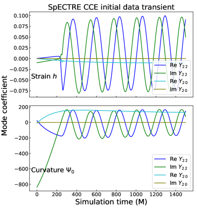
Figure 2: The initial data transient for an example CCE run using worldtube data obtained from a binary black hole simulation SXS:BBH:2096 from the SXS catalog. The dominant modes of the strain and $\Psi_{0}$ display visually apparent drift during the first $\sim 2$ orbits of the inspiral. The initial data transient contaminates the data for the early part of the simulation and leads to a BMS frame shift in the strain waveform. The frame shift can be seen visually from the fact that the $Y_{22}$ mode does not oscillate about 0. The initial data method used for this demonstration is the cubic ansatz initial data described as method 16 below.

Current methods of choosing initial data for $J$ do not represent a snapshot of a much longer simulation, and this gives rise to transients in the resulting strain outputs (see Fig. 2). These initial data transients are analogous to ‘junk radiation’ frequently found in Cauchy simulations, but are somewhat more frustrating for data analysis because the CCE initial data transients tend to have comparatively long timescales. We observe that the strain waveform tends to settle to a suitable state within a few orbits of the start of the simulation. However, when recovering high-fidelity waveforms from an expensive Cauchy simulation, every orbit of trustworthy worldtube data is precious, and it is disappointing to lose those first orbits of data to the initial data transient. It is a topic of ongoing work to develop methods of efficiently generating high-quality initial data for CCE to improve the initial data transient behavior (see Sec. VII.1).

We currently support three methods for generating initial hypersurface data:

1. Keep $\breve{J}$ and $\partial_{\breve{y}}\breve{J}$ consistent with the first timestep of the worldtube data. Use those quantities to fix the angularly dependent coefficients $A$ and $B$ in the cubic initial hypersurface ansatz:

   $$\breve{J}(\breve{y},\breve{\theta},\breve{\phi})=A(\breve{\theta},\breve{\phi})(1-\breve{y})+B(\breve{\theta},\breve{\phi})(1-\breve{y})^{3}.$$ (16)

   This is a similar initial data construction to Bishop et al. (2011), and is chosen to omit any $(1-\breve{y})^{2}$ dependence, which guarantees that no pure-gauge logarithmic terms arise during the evolution Moxon et al. (2020).
   

2. Set the Newman-Penrose quantity $\Psi_{0}=0$ on the initial hypersurface.This amounts to enforcing a second-order nonlinear ordinary differential equation in $y\equiv 1-2R/r$ for $J$, before constructing the coordinate transformation from $x^{\alpha}$ to $\breve{x}^{\breve{\alpha}}$. After some simplification, the expression for $\Psi_{0}$ in Moxon et al. (2020) may be used to show that the equation

   $$\partial_{y}^{2}J=\frac{1}{16K^{2}} \left({\bar{J}}^{2}(\partial_{y}J)^{2}-2(2+J{\bar{J}})\partial_{y}J\partial_{y}{\bar{J}}+J^{2}(\partial_{y}{\bar{J}})^{2}\right)$$

   $$\times\left(-4J-(1-y)\partial_{y}J\right)$$ (17)

   is equivalent to the condition $\Psi_{0}=0$. The initial hypersurface data is generated by first using (2) to perform a radial ODE integration out to $\mathcal{I}^{+}$, with boundary values of $J$ and $\partial_{y}J$ on the initial worldtube. However, the data so generated is not necessarily asymptotically flat, so an angular coordinate transformation is calculated to fix $\breve{J}|_{\mathcal{I}^{+}}=0$. Encouragingly, fixing both (2) and the asymptotic flatness condition also constrains the $(1-y)^{2}$ part of $J$ to vanish, which is sufficient to prevent the emergence of pure-gauge logarithmic dependence during the evolution of $J$.
   

3. Set $\breve{J}=0$ along the entire initial hypersurface. In general, this choice will be inconsistent with the data specified on the worldtube $J|_{\Gamma}$, so it is necessary to construct an angular transformation $x(\breve{x}^{\breve{A}})$ such that $\breve{J}|_{\Gamma}=0$ following the transformation.

Methods 2 and 3 above require the ability to compute the angular coordinate transformation $x^{A}(\hat{x}^{\hat{B}})$ such that

$$0=\breve{J}=\frac{\breve{\bar{b}}^{2}\breve{J}+\breve{a}^{2}\breve{\bar{J}}+2\breve{a}\breve{\bar{b}}\breve{K}}{4\breve{\omega}^{2}}$$ (18)

on some surface. Solving (18) in general would amount to an expensive high-dimensional root-find.

However, in our present application, practical solutions in the wave zone typically have a value of $\breve{J}$ no greater than $\sim 5\times 10^{-3}$, and we should not expect to find a well-behaved angular coordinate transform otherwise. So, we take advantage of the small parameter in the equation to iteratively construct candidate angular coordinate systems that approach the condition (18). Our linearized iteration is based on the approximation

$$\breve{a}_{n+1} =-\frac{1}{2}\frac{\breve{J}_{n}\breve{\omega}_{n}}{\breve{\bar{b}}_{n}\breve{K}_{n}}$$ (19a)

$$\breve{x}^{i}_{n+1}(\breve{x}) =\frac{1}{2}\breve{\eth}^{-1}_{n+1}\left(\breve{a}_{n+1}\breve{\eth}\breve{x}^{i}+\breve{\bar{b}}_{n+1}\breve{\bar{\eth}}\breve{x}^{i}\right),$$ (19b)

for a collection of Cartesian coordinates $\breve{x}^{i}$ that are representative of the angular coordinate transformation (see Sec. III.1).

We find that this procedure typically approaches roundoff in $\sim 10^{3}$ iterations. Despite the crude inefficiency of this approximation, the iterative solve needs to be conducted only once, so it represents only a small portion of the CCE execution time for the initial data methods that take advantage of it.

In practical investigations, it has been found that most frequently the simplest method of an inverse cubic ansatz (1. above) performs best in various measures of asymptotic data quality Mitman et al. (2021). However, because the reasons for the difference in precision for different initial data schemes are not currently well understood, we believe it useful to include descriptions of all viable methods.

III Implementation details and Numerical optimizations

Much of the good performance of the SpECTRE CCE system is inherited from the shared SpECTRE infrastructure. In particular, the SpECTRE data structures offer easy interfaces to aggregated allocations (which limit expensive allocation of memory), fast vector operations through the interface with the open source Blaze library Bla , and rapid SWSH transforms via the open source libsharp library. Further, we take advantage of per-core caching mechanisms to avoid recomputing common numerical constants, such as spectral weights and collocation values.

However, in addition to establishing ambitious “best practices” for the mechanical details of the software development, we have implemented numerical optimizations specialized to calculations in the CCE system. We give a brief explanation of the techniques we use to improve performance of angular interpolation in Sec. III.1, which is required to perform the gauge transformation discussed in Sec. II.4. In Sec. III.2, we explain our methods for efficiently performing the hypersurface integrals in our chosen Legendre-Gauss-Lobatto pseudospectral representation.

III.1 Angular interpolation techniques using spin-weighted Clenshaw algorithm

The Clenshaw recurrence algorithm is a fast method of computing the sum over basis functions,

$$f(x)=\sum_{n=0}^{N}a_{n}\phi_{n}(x),$$ (20)

provided the set of basis functions $\phi_{n}$ obeys a standard form of a three-term recurrence relation common to many polynomial bases. In particular, it is assumed that $\phi_{n}$ may be written as,

$$\phi_{n}(x)=\alpha_{n}(x)\phi_{n-1}(x)+\beta_{n}(x)\phi_{n-2}(x),$$ (21)

for some set of easily computed $\alpha_{n}$ and $\beta_{n}$.

The algorithm for computing the full sum $f(x)$ Press et al. (2007) is then to compute the set of quantities $y_{n}$ for $n\geq 1$, where $y_{n}$ is

$$y_{N+2}(x)= y_{N+1}(x)=0$$ (22a)

$$y_{n}(x)= \alpha_{n+1}(x)y_{n+1}(x)$$

$$+\beta_{n+2}(x)y_{n+2}(x)+a_{n}$$ (22b)

Once the last two quantities in the chain $y_{1}(x)$ and $y_{2}(x)$ are determined, the final sum is obtained from the formula

$$f(x)=\beta_{2}(x)\phi_{0}(x)y_{2}(x)+\phi_{1}(x)y_{1}(x)+a_{0}\phi_{0}(x).$$ (23)

We use the Clenshaw method for interpolating SWSH data to arbitrary points $x$ on the sphere. For spherical harmonics, it is successive values of $\ell$ that have convenient three-term recurrence relations, so the lowest modes in the recursion are $Y_{|m|,m}(\theta,\phi)$ and $Y_{|m|+1,m}(\theta,\phi)$. The values of $\alpha_{\ell,m}(\theta,\phi)$ and $\beta_{\ell,m}(\theta,\phi)$ are cached for the target interpolation points, and the source collocation values are transformed to spectral coefficients $a_{\ell,m}$. The Clenshaw algorithm can be applied directly at each of the target points $(\theta,\phi)$, to obtain the values $f(\theta,\phi)$. Note that the step of caching the $\alpha_{\ell,m}(\theta,\phi)$ and $\beta_{\ell,m}(\theta,\phi)$ is primarily useful for interpolating multiple functions to the same grid; if only one function is needed for each grid, there will be little gain in caching $\alpha$ and $\beta$, as they would each be evaluated only once in a given recurrence chain.

In Appendix C, we give full details of the specific recurrence relations that can be used to efficiently calculate the Clenshaw sum for SWSH, as well as additional recurrence relations that improve performance when moving between the $m$ modes. For the remaining discussion it is convenient to define a few auxiliary variables that are used in the formulas for the SWSH recurrence:

$$a =|s+m|$$ (24a)

$$b =|s-m|$$ (24b)

$$\lambda =\begin{cases}0,&s\geq-m\\ s+m,&s<-m\end{cases}$$ (24c)

The step-by-step procedure for efficiently interpolating a spin-weighted function represented as a series of spin-weighted spherical harmonic coefficients to a set of target collocation points $(\theta_{i},\phi_{i})$ is then:

1. Assemble the lookup table of required ($\alpha_{\ell}^{(a,b)}(\theta)$, $\beta_{\ell}^{(a,b)}$, $\lambda_{m}$):

   1. For each $m\in[-\ell_{\max},\ell_{\max}]$ there is a pair $(a,b)$ from (24) to be computed. Note that $\alpha^{(a,b)}_{\ell}$ must be cached separately for each target point, but $\beta^{(a,b)}_{\ell}$ does not depend on the target coordinates.

2. For $m\in[0,\ell_{\max}]$:

   1. If $|s|\geq|m|$: Determine ${}_{s}Y_{|s|,m}(\theta,\phi)$ from direct evaluation of (59) with (C.0.1) and ${}_{s}Y_{|s|+1,m}(\theta,\phi)$ from (68); Store ${}_{s}Y_{|s|,m}(\theta,\phi)$ for recursion if $|s|=|m|$.

   2. If $|m|>|s|$: Determine ${}_{s}Y_{|m|,m}(\theta,\phi)$ from recurrence (67) and ${}_{s}Y_{|m|+1,m}(\theta,\phi)$ from (68). Store ${}_{s}Y_{|m|,m}(\theta,\phi)$ for recursion.

   3. Perform the Clenshaw algorithm to sum over $l\in[\min(|s|,|m|),\ell_{\max}]$, using the spectral coefficients $a_{\ell m}$, the precomputed $\alpha_{\ell}^{(a,b)}$ and $\beta_{\ell}^{(a,b)}$ recurrence coefficients, and the first two harmonics in the sequence computed from the previous step.

3. For $m\in[-1,-\ell_{\max}]$, repeat the substeps of step 2, but for the negative set of $m$’s.

Although the procedure for interpolation is performed efficiently, there are a number of details of the implementation of the angular coordinate transformation that must be handled carefully.

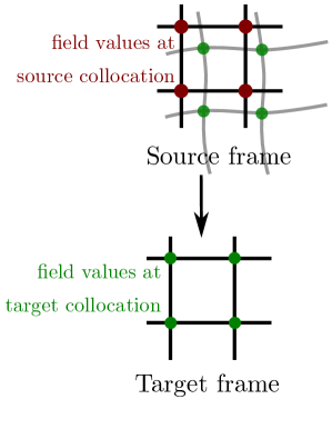
Figure 3: An illustration of the interpolation reasoning for pseudospectral methods. The input to the interpolation is the field values at the collocation points in the source frame, and we wish to determine the field values for the same function at the collocation points in the target frame, which will be at non-collocation points in the source frame coordinates. Therefore, the interpolation seeks to calculate the field value at points $x(\hat{x})$ in the source frame, for all collocation points $\hat{x}$ in the target frame.

First, it is important to note the counterintuitive nature of the set of coordinate functions we require for the interpolation. In both the source frame and the target frame, we use a pseudospectral grid, evenly spaced in $\phi$, and at Legendre-Gauss points in $\theta$. When interpolating, we require the location in the source frame coordinates of the target frame collocation points. Therefore, when expressed as a function over collocation points, the function that we use for interpolation is $x^{A}(\hat{x}^{A})$. We have found this feature of the interpolation for pseudospectral methods easy to misremember, so we have included Fig. 3 to assist in recalling the correct reasoning.

Most of the quantities that we wish to interpolate have nonzero spin-weight, so do not transform as scalars. Instead, their transformation involves factors of the spin-weighted angular Jacobians (13). The tensor transformations for each of the relevant quantities at the worldtube boundary are given in (15). For illustration, let us discuss the transformation of the spin-weight 2 scalar $\breve{J}$:

$$\breve{J}=\frac{\breve{\bar{b}}^{2}J+\breve{a}^{2}\bar{J}+2\breve{a}\breve{\bar{b}}K}{4\breve{\omega}}$$ (25)

It is important to note that at the start of the transformation procedure, we have the values of $J$ on the source grid $x^{A}$ and the values of $\breve{a}$, $\breve{b}$, and $\breve{\omega}$ on the target grid $\breve{x}^{\breve{A}}$ (the Jacobians are derivatives of $x(\breve{x})$; see Fig. 3).

The spin-weighted interpolation procedure can be performed only on quantities that are representable by the SWSH basis. We can store non-representable quantities (including, e.g. the angular coordinates themselves) on our chosen angular grid, but we cannot perform a SWSH transform on such quantities, so we cannot interpolate them using pseudospectral methods with any predictable accuracy. Inconveniently, we are burdened with a number of quantities that are not representable on the SWSH basis. Immediately after interpolation, $J(x^{A}(\breve{x}^{\breve{A}}))$ is not representable on the basis corresponding to the new grid because the Jacobian factors have not yet been applied. Similarly, the Jacobian factors $\breve{a}$ and $\breve{b}$ are not representable on the SWSH basis whenever the angular transform is not trivial.

Accordingly, for our example of $\breve{J}$, we must apply the transformation operations in a specific sequence:

1. Interpolate $J(x^{A})$ and $K(x^{A})$ to $J(x^{A}(\breve{x}^{\breve{A}}))$ and $K(x^{A}(\breve{x}^{\breve{A}}))$.

2. Multiply the result by the Jacobian factors that appear in (25).

We meet a similar complication when manipulating the evolved angular coordinates $x^{A}(\breve{u},\breve{x}^{\breve{A}})$. The angular coordinates are not representable on the SWSH basis, yet we must take angular derivatives of the angular coordinates to determine the Jacobian factors (13). The method we use to evade the problems for the angular coordinate representation is to introduce a unit sphere Cartesian representation of the angular coordinates:

$$x_{\text{unit}} =\sin\theta\cos\phi,$$ (26a)

$$y_{\text{unit}} =\sin\theta\sin\phi,$$ (26b)

$$z_{\text{unit}} =\cos\theta.$$ (26c)

The evolution equation for the unit sphere Cartesian representation is then derived from the angular coordinate evolution equation (12).

$$\partial_{\breve{u}}x^{i}_{\text{unit}} =\mathcal{U}_{0}^{\breve{A}}\partial_{\breve{A}}x^{i}_{\text{unit}}$$

$$=\frac{1}{2}\left(\mathcal{U}_{0}\breve{\bar{\eth}}x^{i}_{\text{unit}}+\bar{\mathcal{U}}_{0}\breve{\eth}x^{i}_{\text{unit}}\right).$$ (27)

The main advantage of promoting the angular coordinates $x^{A}(\breve{u},\breve{x}^{\breve{A}})$ to their unit sphere Cartesian analogs is that the Cartesian coordinates $x^{i}$ are spin-weight 0 and so we can quickly and accurately evaluate their angular derivatives.

The spin-weighted Jacobian factors (13) are then calculated as

$$\breve{a}=\breve{\eth}x^{i}\partial_{i}x^{A}q_{A},$$ (28a)

$$\breve{b}=\breve{\bar{\eth}}x^{i}\partial_{i}x^{A}q_{A},$$ (28b)

where the factors $\partial_{i}x^{A}$ are the Cartesian-to-angular Jacobians in the source frame, so are analytically computed as

$$\partial_{x}\theta =\cos[\phi(\hat{x}^{\hat{A}})]\cos[\theta(\hat{x}^{\hat{A}})],$$ (29a)

$$\partial_{x}\phi =-\sin[\phi(\hat{x}^{\hat{A}})]/\sin[\theta(\hat{x}^{\hat{A}})],$$ (29b)

$$\partial_{y}\theta =\cos[\theta(\hat{x}^{\hat{A}})]\sin[\phi(\hat{x}^{\hat{A}})]$$ (29c)

$$\partial_{y}\phi =\cos[\phi(\hat{x}^{\hat{A}})]/\sin[\theta(\hat{x}^{\hat{A}})],$$ (29d)

$$\partial_{z}\theta =-\sin[\theta(\hat{x}^{\hat{A}})],$$ (29e)

$$\partial_{z}\phi =0.$$ (29f)

III.2 Rapid linear algebra methods for radial integration

SpECTRE CCE uses a Legendre Gauss-Lobatto spectral representation for the radial dependence of the spin-weighted scalars on its domain. The use of spectral methods allows rapid integration of the radial differential equations of the hierarchical CCE system (9). The numerical methods we employ in this section are not themselves new, but they have not previously been applied to efficiently solving the CCE system of equations.

Each of the angular derivatives that appears in the hierarchy of radial differential equations is first evaluated by the procedure described around Eq. (6): perform a spin-weighted spherical harmonic transform using libsharp, multiply by $\sqrt{(\ell-s)(\ell+s+1)}$ in the modal basis for the $\breve{\eth}$ and $-\sqrt{(\ell+s)(\ell-s+1)}$ for $\breve{\bar{\eth}}$, and recover the nodal representation of the derivative with an inverse spin-weighted transform. Using these nodal values of the angular derivative terms , we may then directly compute each of the right-hand sides of the radial differential equations over the nodal grid. Therefore, for each of the radial differential equations, the problem reduces to a collection of radial ODE solves.

The spectral representation in the radial direction allows the further simplification of determining linear operators that correspond to indefinite integration. Given the function $f$ expressed in the modal representation

$$f(\breve{y})=\sum_{n}a_{n}P_{n}(\breve{y}),$$ (30)

we seek the integration matrix $I$ such that

$$\sum_{n}a_{n}\int^{\breve{y}}P_{n}(\breve{y})=\sum_{n}(I\cdot a)_{n}P_{n}(\breve{y}),$$

$$\Longrightarrow\quad \sum_{n}a_{n}P_{n}(\breve{y})=\sum_{n}(I\cdot a)_{n}\partial_{\breve{y}}P_{n}(\breve{y}),$$ (31)

The relevant identity for Legendre polynomials that we use to determine the integration matrix $I$ is

$$P_{n}(\breve{y})=\frac{1}{2n+1}\frac{d}{d\breve{y}}\left[P_{n+1}(\breve{y})-P_{n-1}(\breve{y})\right].$$ (32)

By integrating both sides of this equation and applying the result to the modal representation (30), we find the almost-tridiagonal indefinite integration matrix for the spectral representation

$$I=\begin{bmatrix}-1&1&-1&1&\cdots&(-1)^{n+1}\\ -1&0&-1/3&0&\cdots&0\\ 0&1&0&-1/5&\cdots&0\\ \vdots&\vdots&\ddots&\ddots&\ddots&\vdots\\ 0&0&\cdots&1/(2n-1)&0&-1/(2n+3)\end{bmatrix}.$$ (33)

Here the first row is chosen to zero the function at the innermost gridpoint (at $\breve{y}=-1$). It is convenient to generate linear operators acting entirely on the nodal representation. These are composed as $M^{-1}IM$, where $M$ is the linear operator that maps the nodal representation to the modal representation. We may then add an integration constant freely to the result of the indefinite integration operator in the nodal representation to satisfy the boundary conditions.

Two of the five equations (those that determine $\breve{\beta}$ and $\breve{U}$) take the simple form

$$\partial_{\breve{y}}f=S_{f}.$$ (34)

The radial ODE solves for these cases are a straightforward application of the nodal integration matrix $M^{-1}IM$ using (33). In the CCE system, the choice to zero the value at the innermost boundary point ensures that we may impose the boundary conditions for the worldtube quantities $\breve{\beta}|_{\Gamma}$ and $\breve{U}|_{\Gamma}$ by adding the appropriate boundary value to all points along the radial rays for each angular point on the boundary.

Two more of the radial differential equations (those that determine $\breve{Q}$ and $\breve{W}$) take the form

$$(1-\breve{y})\partial_{\breve{y}}f+2f=S_{f}.$$ (35)

This case requires more care than the original indefinite integral, but the full integration matrix is still readily calculable for arbitrary Legendre order $n$.

Considering again the modal representation (30), we wish to find the linear operator $K$ such that

$$\sum_{n}a_{n}P_{n}(\breve{y})=\sum_{n}(K\cdot a)_{n}[(1-\breve{y})\partial_{\breve{y}}P_{n}(\breve{y})+2P_{n}(\breve{y})].$$ (36)

The operator $K$ is the inverse of the operator in Eq. (35).

We will again make use of the integration matrix $I$ (33). We also require the inverse of the matrix $C$ associated with multiplication by $(1-\breve{y})$:

$$\sum(C\cdot a)_{n}P_{n}(\breve{y})=\sum a_{n}(1-\breve{y})P_{n}(\breve{y}).$$ (37)

The matrix $C$ is derived by algebraic manipulations of Bonnet’s recursion formula for Legendre polynomials

$$(n+1)P_{n+1} =(2n+1)\breve{y}P_{n}-nP_{n-1}$$

$$\Rightarrow(1-\breve{y})P_{n} =-\frac{n+1}{2n+1}P_{n+1}+P_{n}-\frac{n}{2n+1}P_{n-1}$$ (38)

Therefore, composing the operations of $C$ and $I$, we find

$$\sum_{n}((C+2I)\cdot a)_{n}P_{n}(\breve{y})=\sum_{n}(I\cdot a)_{n}\left[(1-\breve{y})\partial_{\breve{y}}P_{n}+2P_{n}\right]$$ (39)

and

$$K=I\cdot(C+2I)^{-1}$$ (40)

To compute $K$ in practice, we determine the values of $C$ and $I$ analytically, then perform a single numerical inversion to finish the computation of (40). Boundary conditions then determine the quadratic part of the solution, so are imposed by adding the appropriate $b(\breve{\theta},\breve{\phi})(1-\breve{y})^{2}$ contribution along each radial ray.

Importantly, for both of the above types of the radial ODE solve, the integration matrix in question is independent of the values of the fields. So, at the start of the simulation, we precompute and store the necessary integration matrices, reducing each of the ODE solves described above to a matrix-vector multiplication for each radial ray. In SpECTRE, these matrix-vector product calculations are optimized via the vector intrinsic library libxsmm Lib (b).

The final type of radial differential equation appears only in the equation that determines $H$. This type is more complicated:

$$(1-\breve{y}) \partial_{\breve{y}}f+[1+(1-\breve{y})L^{G}L^{J}]f+(1-\breve{y})\bar{L}^{G}L^{J}\bar{f}=S,$$ (41)

in which the $L$ factors depend on the field quantities of the current hypersurface. In this case, there is little hope of determining an elegant simplification using the modal basis. In any case, there would be no opportunity for caching and reusing an integration matrix, as the differential operator that acts on $f$ depends on the other fields on the hypersurface. So, for the integration of the $H$ equation, we decompose the complex linear differential equation into a real linear equation on vectors of length $2n$:

$$\bigg{\{}\begin{bmatrix}(1-\breve{y})\partial_{\breve{y}}+1&0\\ 0&(1-\breve{y})\partial_{\breve{y}}+1\end{bmatrix}\\ +(1-\breve{y})\begin{bmatrix}\text{Re}(L^{J})\text{Re}(L^{G})&\text{Re}(L^{J})\text{Im}(L^{G})\\ \text{Im}(L^{J})\text{Re}(L^{G})&\text{Im}(L^{J})\text{Im}(L^{G})\end{bmatrix}\bigg{\}}\begin{bmatrix}\text{Re}(f)\\ \text{Im}(f)\end{bmatrix}\\ =\begin{bmatrix}\text{Re}(S)\\ \text{Im}(S)\end{bmatrix},$$ (42)

where the multiplication by $(1-\breve{y})$ and differentiation $\partial_{\breve{y}}$ are understood to represent linear operators on the Legendre Gauss-Lobatto nodal representation. We then solve (42) by numerically computing the linear operator along each radial ray and performing an aggregated linear solve via LAPACK. Boundary conditions are imposed as usual by setting the first row of the operands $\text{Re}(S)$ and $\text{Im}(S)$ to the desired boundary value before the operation, and adjusting the first and $(n+1)$ row of the linear operator to be equivalent to the first and $(n+1)$ row of the identity matrix.

IV Parallelization and modularity

Because of the dependence of the gauge transformation at the inner boundary on the field values at $\mathcal{I}^{+}$ needed to establish an asymptotically flat gauge, the opportunities for subdividing the CCE domain for parallelization purposes are limited. However, we are able to take advantage of the task-based parallelism in SpECTRE to: a) parallelize independent portions of the CCE information flow, and b) efficiently parallelize the CCE calculation with a simultaneously running Cauchy simulation.

IV.1 Component construction

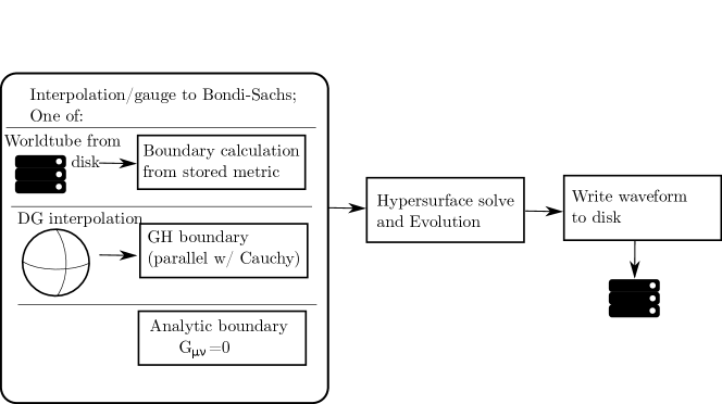
Figure 4: Components of the CCE task-based parallelism system. The worldtube component (left) is modular and can be switched out according to the desired source of worldtube data. We currently support reading worldtube data from disk, interpolating worldtube data from a simultaneously running Generalized Harmonic system in SpECTRE, or computing analytic boundary data from a known solution or approximation to the Einstein field equations.

In SpECTRE, we refer to the separate units of the simulation that may be executed in parallel via task-based parallelism as components. For instance, in the near-field region in which the domain can be parallelized among several subregions of the domain, each portion of the domain is associated with a component.

For SpECTRE CCE, we use three components (in addition to components that are used for the Cauchy evolution): one component for the characteristic evolution, another component dedicated to providing boundary data on the worldtube, and a third component for writing results to disk.

Much of the efficiency and precision of the SpECTRE CCE system comes from the ability to cover the entire asymptotic domain from the worldtube $\Gamma$ to $\mathcal{I}^{+}$ with a single spectral domain. In principle, there may be opportunity to parallelize multiple radial shells of the computation, but in practice our initial assessments indicated that there would be little gain for the typical gravitational wave extraction scenario. First, there is a significant constraint that comes from the asymptotic flatness condition — the gauge transformation throughout the domain on a given hypersurface depends on the asymptotic value $\mathcal{U}|_{\mathcal{I}^{+}}$ on the same hypersurface, which forces a significant portion of the computation to serial execution. Additionally, we have seen very rapid convergence in the number of radial points used for the CCE system, so it is unlikely that subdividing the domain radially would offer much additional gain for the typical use case.

Therefore, the entire characteristic evolution system is assigned to a single component, and represents the computational core of the algorithm. The evolution component is responsible for

• The angular gauge transformation and interpolation (via Clenshaw recurrence)

• The calculation of the right-hand sides of the set of hierarchical equations (9)

• The integration of each of the radial ODEs

• The time interpolation and preparation of waveform data

The core evolution component performs no reads from or writes to the filesystem, which ensures that the expensive part of the computation will not waste time waiting for potentially slow disk operations.

The second component used in CCE is the worldtube component. A worldtube component is responsible for:

• Collecting the Cauchy worldtube metric and its derivatives from an assigned data source

• Interpolating the data to time steps appropriate to the CCE evolution system

• Performing the transformation to the Bondi-Sachs-like coordinate system on the worldtube

The user has a choice of several different worldtube components, each of which corresponds to a different source of the metric quantities on the worldtube. Worldtube components are available that:

• Read worldtube data directly from disk

• Accept interpolated data from a simultaneously running Cauchy execution in SpECTRE

• Calculate worldtube data from an analytically determined metric on the boundary

Our methods for reading from disk are currently optimized for easily reading worldtube data written by SpEC, but our worldtube module should accept data from any code that can produce the spacetime metric and its first derivatives decomposed into spherical harmonic modes.

Finally, there is a generic observer component that handles the output of the waveform data to disk. When CCE is simultaneously running with a Cauchy evolution, there will be additional components running in parallel with the CCE components, such as components that perform the Cauchy evolution, components that search for apparent horizons, and components that write simulation data to disk. The division of the CCE pipeline into parallel components is illustrated in Fig. 4.

IV.2 Independently stepped interface with Cauchy simulation

Because the Cauchy-characteristic evolution system does not have much opportunity to parallelize internally, we need to ensure that its serial execution is optimized. Our goal is that when running simultaneously with the highly parallel discontinuous Galerkin system used for the Generalized Harmonic evolution, the CCE system does not impose any significant runtime penalty.

An important contribution to the efficiency of the CCE system is that the solutions to the Einstein field equations are smooth and slowly varying in time. As a result, the spectral methods used in CCE converge rapidly, and the scales that we seek to resolve with the time-stepper are primarily on orbital timescales. Therefore, we anticipate that the CCE system should be able to take far larger timesteps than the Generalized Harmonic system running in concert, and it will be important for the overall efficiency of the extraction pipeline to adjust the time steps of the CCE evolution independently of the time step of the Generalized Harmonic system Lindblom et al. (2006).

Our implementation permits the CCE step size to vary independently of other time scales in the simulation, and the step size can be chosen according to estimates of the time stepper residuals. Those estimates are frequently obtained by comparing the results of time steppers of different orders, either via embedded methods Harier et al. (1993) for substep integrators, or by varying the number of points used in the arbitrary-sized multistep methods (LMM) Throwe and Teukolsky (2020) often used in SpECTRE.

The CCE worldtube component receives the metric and its first time derivatives from the Generalized Harmonic system. It then uses dense output to generate evenly spaced data sets and barycentric rational interpolation Floater and Hormann (2007) to generate values at the time points required by the CCE evolution system. This technique ensures that the interpolated time points will have a precision associated with the scale of stepper residuals of the Generalized Harmonic system.

To demonstrate the usefulness of our variable step size implementation, we have performed a simple evolution in SpECTRE using input from a SpEC binary black hole simulation, and compared the size of the time steps between the SpEC evolution system and the SpECTRE CCE system. In Fig. 5 we show the respective step size of a globally stepped Generalized Harmonic system in SpEC and the step size of the SpECTRE CCE system using an adaptive step size based on time stepper residuals.

For the evolution system in SpECTRE, we will have the opportunity to perform local time-stepping for separate elements in the Generalized Harmonic domain as well, which will allow the elements in direct communication with the CCE system to take larger steps. However, even for modest resolution in the SpECTRE Generalized Harmonic system, and for a 100M worldtube radius, we should expect the Generalized Harmonic system to still take $\mathcal{O}(10)$ steps per $M$ of evolution for an Adams-Bashforth order 3 scheme, so the CCE system should still benefit from an independently chosen step size.

The examples in this section emphasize the value in permitting the CCE system to choose its own step size — the smoothness of the solution across the asymptotic null hypersurface ensures that CCE can comfortably take far larger time steps than its partner Generalized Harmonic system. The larger time steps then permit either a far faster extraction in the case of a standalone CCE run, or permit the CCE system to make negligible impact on the overall runtime when evolved in tandem with the Generalized Harmonic evolution in SpECTRE.

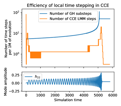
Figure 5: A comparison of the number of substeps taken per $1\,M$ of simulation time in the SpEC Generalized Harmonic evolution (with Dormand-Prince-5 substep method) to the number of steps taken in the CCE system (with Adams-Bashforth order 3 linear multistep method). We choose to compare the number of substeps to the number of LMM steps, as it most closely represents the factor of speedup in the CCE system as compared to a system in which CCE is forced to take identical steps to the GH system that supplies its worldtube data, i.e. a global time-stepping method across all systems. The SpECTRE system chooses steps in discrete factors of 2 as a simplification to the time-stepping infrastructure and to maintain globally agreed-upon ‘slabs’ of the evolution, so the time steps chosen in our CCE implementation jump by factors of 2 during transitions.The bottom plot shows the dominant gravitational waveform mode for reference.

V Battery of tests

V.1 Barkett test collection

In Barkett et al. (2020), we described a series of demanding tests for verifying the correctness and efficiency of the SpEC implementation of CCE. We have reimplemented all five of those analytic tests for SpECTRE CCE, and similarly verified the correctness and convergence properties of the new implementation. Here, we briefly summarize the salient features of each of the test cases and present the results from applying the collection of tests to our new implementation in SpECTRE. Please refer to Barkett et al. (2020) for complete details regarding the formulation of the tests.

Each test generates Cauchy worldtube metric and its derivatives on a chosen worldtube and uses a custom version of the CCE worldtube component to provide the Cauchy worldtube metric and its derivatives to the characteristic evolution component. Otherwise, the remainder of the pipeline operates precisely as it would if extracting waves from data generated by a full Cauchy evolution (see Fig. 4). The analytic tests provide a prediction for the asymptotic Bondi-Sachs news function, which is then compared against the extracted news function to determine a residual and evaluate the precision of the CCE system.

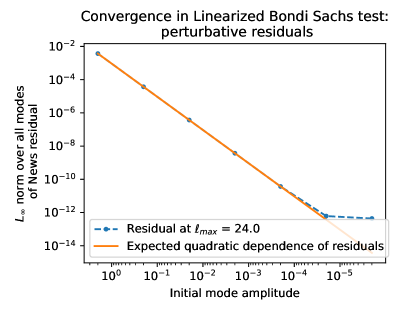
Figure 6: Residual obtained by subtracting the numerical SpECTRE CCE news from the linearized Bondi-Sachs news. The residual follows closely the expected perturbative residual $\propto\alpha^{2}$ for amplitude $\alpha$, until the time stepper residual dominates at $\sim 10^{-12}$ (The absolute tolerance of the time stepperis chosen to be $10^{-13}$ in these tests and run for a duration of $5/\nu$).

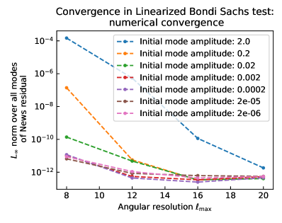
Figure 7: Numerical residual in the Linearized Bondi-Sachs test, obtained by subtracting the extracted news from its value at the maximum resolution ($\ell_{\text{max}}=24$) for each given amplitude.

Linearized Bondi-Sachs:

This solution expands the Bondi-Sachs metric (II.2) around the flat space solution, and was first derived in Bishop (2005). The spin-weighted scalars that determine the metric are expanded in modes as

$$J_{\text{lin}\,\ell m} =\sqrt{(\ell+2)!/(\ell-2)!}\;{}_{2}Z_{\ell m}\text{Re}[J_{\ell}(r)e^{i\nu u}]$$ (43a)

$$U_{\text{lin}\,\ell m} =\sqrt{\ell(\ell+1)}\;{}_{1}Z_{\ell m}\text{Re}[U_{\ell}(r)e^{i\nu u}]$$ (43b)

$$\beta_{\text{lin}\,\ell m} ={}_{0}Z_{lm}\text{Re}[\beta_{\ell}(r)e^{i\nu u}]$$ (43c)

$$W_{\text{lin}\,\ell m} ={}_{0}Z_{lm}\text{Re}[W_{\ell}(r)e^{i\nu u}],$$ (43d)

where $\nu$ is a user-defined frequency and each radially dependent $\ell$-mode of the solution is specified by analytic calculation via the expansion of the Einstein field equations in the Bondi-Sachs gauge, and the spin-weighted spherical harmonic functions ${}_{s}Z_{\ell m}$ from Bishop (2005) are

$${}_{s}Z_{\ell m}=\begin{cases}\frac{i}{\sqrt{2}}\left[(-1)^{m}{}_{s}Y_{\ell m}-{}_{s}Y_{\ell-m}\right],&m<0,\\ {}_{s}Y_{\ell 0},&m=0,\\ \frac{1}{\sqrt{2}}\left[{}_{s}Y_{\ell m}+(-1)^{m}{}_{s}Y_{\ell-m}\right],&m>0.\end{cases}$$ (44)

The asymptotic news function is then

$$N_{\text{lin}\,\ell m}= \text{Re}\left[e^{i\nu u}\lim_{r\rightarrow\infty}\left(\frac{\ell(\ell+1}{4}J_{\ell}-\frac{i\nu r^{2}}{2}J_{\ell,r}+\beta_{\ell}\right)\right]$$

$$\hskip 14.22636pt\times\sqrt{\frac{(\ell+2)!}{(\ell-2)!}}{}_{2}Z_{\ell m}.$$ (45)

As in the SpEC implementation, we consider only $\ell=2$ and $\ell=3$ modes, for which the full radial dependence is given in Bishop (2005); Barkett et al. (2020). Because the above linearized Bondi-Sachs expressions are valid only to first order in the perturbation amplitude $\alpha$, but CCE evolves the full nonlinear Einstein equations, the difference between the linearized solution and CCE should depend quadratically on the amplitude $\alpha$. In Fig. 6, we plot this difference versus $\alpha$, and we recover the expected quadratic dependence, so that the relative residual is proportional to the perturbation amplitude $\alpha$. Figure 7 shows the convergence of the CCE news with angular resolution $\ell_{\text{m}ax}$: plotted is the difference between the CCE news at a given $\ell_{\text{m}ax}$ and the CCE news at $\ell_{\text{m}ax}=24$.

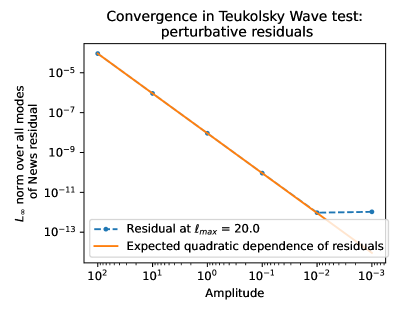
Figure 8: Residual obtained by subtracting the SpECTRE CCE news from the news computed from an $(\ell,m)=(2,0)$ Teukolsky wave. The residual follows closely the expected perturbative residual $\propto\alpha^{2}$ for amplitude $\alpha$, until the time stepper residual dominates at $\sim 10^{-12}$ (The absolute tolerance of the time stepper is chosen to be $10^{-13}$ in these tests and run for duration $5\tau$).

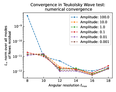
Figure 9: Numerical residual in the Teukolsky wave test, obtained by subtracting the extracted news from its value at the maximum resolution ($\ell_{\text{max}}=20$) for each given amplitude.

Teukolsky wave:

A linearized perturbation on a flat background is evaluated on the worldtube and compared against the predicted asymptotic news. We use the outgoing form of the linearized metric given in Teukolsky (1982); Barkett et al. (2020):

$$ds^{2}= -dt^{2}+(1+f_{rr})dr^{2}+2Bf_{r\theta}rdrd\theta$$

$$+2Bf_{r\phi}r\sin\theta drd\phi+\left(1+Cf_{\theta\theta}^{(1)}+Af_{\theta\theta}^{(2)}\right)r^{2}d\theta^{2}$$

$$+2(A-2C)f_{\theta\phi}r^{2}\sin\theta d\theta d\phi$$

$$+\left(1+Cf_{\phi\phi}^{(1)}+Af_{\phi\phi}^{(2)}\right)r^{2}\sin^{2}\theta d\phi^{2},$$ (46)

where the functions $A$, $B$, and $C$ are determined by the arbitrary wave profile function $F(u)=F(t-r)$:

$$A =\frac{1}{r^{3}}\left(\partial_{u}^{2}F+3r^{-1}\partial_{u}F+3r^{-2}\partial_{u}F\right)$$ (47a)

$$B =-\frac{1}{r^{2}}\left(\partial_{u}^{3}F+3r^{-1}\partial^{2}_{u}F+6r^{-2}\partial_{u}F+6r^{-3}\partial_{u}F\right)$$ (47b)

$$C =\frac{1}{4r}\big{(}\partial_{u}^{4}F+2r^{-1}\partial^{3}_{u}F+9r^{-2}\partial^{2}_{u}F$$

$$\hskip 56.9055pt+21r^{-3}\partial_{u}F+21r^{-4}F\big{)},$$ (47c)

and the $f_{ij}^{(n)}$ functions are tensor harmonic functions determined by the choice of ${}_{s}Y_{\ell m}$ modes. We follow Barkett et al. (2020) and choose a strictly outgoing ${}_{2}Y_{20}$ mode, and for that choice of solution, the asymptotic news is

$$N=\frac{3}{4}\sin^{2}\theta\,\partial_{u}^{5}F(u).$$ (48)

We also choose a Gaussian wave profile $F(u)=\alpha e^{-u^{2}/\tau^{2}}$ with amplitude $\alpha$ and width $\tau$.

As in the Linearized Bondi-Sachs solution, the analytic solution for the Teukolsky wave generates a nontrivial waveform, but the solution is perturbative. Because CCE evolves the full nonperturbative Einstein equations, the difference between CCE and the perturbative solution should scale as $\alpha^{2}$. We show the convergence of the residual with diminishing amplitude in Fig. 8, and in Fig. 9 we show the convergence of the numerical residuals determined by comparing to the highest resolution run conducted ($\ell_{\text{max}}=20$).

Test name	Parameters tested	Maximum residual
Rotating Schwarzschild	$\ell_{\text{max}}\in[8,24];\omega\in[0.1,0.8]$	$2.94\times 10^{-11}$
Gauge Wave	$\ell_{\text{max}}\in[8,24];\alpha\in[0.01,10.0]$	$4.05\times 10^{-12}$

Table 1: Maximum residuals across the explored parameter space for the rapidly converging test cases.

Rotating Schwarzschild:

We generate worldtube data from the Schwarzschild metric in Eddington-Finkelstein coordinates, with an angular coordinate transformation $\phi\rightarrow\phi+\omega u$ applied:

$$ds^{2}= -\left(1-\frac{2M}{r}-\omega^{2}r^{2}\sin^{2}\theta\right)du^{2}-2dudr$$

$$+2\omega r^{2}\sin^{2}\theta dud\phi+r^{2}\sin^{2}\theta d\Omega^{2}.$$ (49)

This test case produces no waves, so we expect to recover news $N=0$ from the CCE system. For this test case, we find extremely small residuals across the parameter space that we explored. No run resulted in any mode of the news exceeding ${}\sim 10^{-11}$; this test case is included in summary table 1.

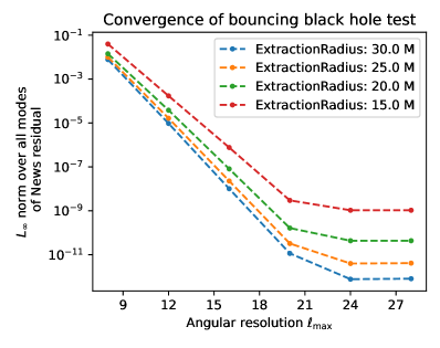
Figure 10: Convergence of SpECTRE CCE for the bouncing black hole test across various extraction radii. Here, we have set the absolute tolerance of the stepper residual to $10^{-12}$ to ensure that the residuals are associated only with the spatial resolution. At an extraction radius of $15M$,the convergence saturates slightly early, at around $\sim 10^{-9}$. However, at even modestly larger extraction radii, the SpECTRE CCE system approaches the expected truncation scale of the spectral scheme.

Bouncing Schwarzschild black hole:

The worldtube data for the bouncing black hole test is similar conceptually to the Rotating Schwarzschild test. However, instead of performing an angular coordinate transformation, here we apply a time dependent linear transformation to the Kerr-Schild coordinate system $(t,x,y,z)$:

$$x\rightarrow x+a\sin^{4}(2\pi t/b).$$ (50)

As in the Rotating Schwarzschild test, the expected result of the CCE system is zero news, since the solution is simply Schwarzschild in an oscillating coordinate system. For our tests, we choose an oscillation amplitude $a=2M$ and period $b=40M$.

In practice, the bouncing black hole test has proven to be a far more demanding test of the CCE wave extraction system than many of the other tests. A naive examination of individual Bondi-Sachs scalars in this scenario would lead one to believe that there is wave content in the system — it is only through the full nonlinear simulation that the CCE system is able to resolve the motion as a pure-gauge effect and cancel all of the contributions in the final value of the news. We show the convergence of the SpECTRE CCE system for the bouncing Schwarzschild black hole test in Fig. 10.

Because the bouncing black hole test has proven to be such a thorough test of CCE, we have chosen this test case as a benchmark system to compare the SpEC and SpECTRE simulation codes, both for speed and precision. In Figs. 11 and 12 we show the relative precision and wallclock execution times for the two systems, for similar parameters of the test system.

We use a somewhat more demanding error measure than in the previous publication Barkett et al. (2020): we take the maximum error over all extracted modes, instead of examining particular modes and potentially neglecting the highest modes that can accumulate nontrivial value. The angular resolution plotted here is the $\ell_{\text{max}}$ used during the worldtube transformation phase of the computation, as that is the most demanding part of the calculation for angular resolution. The SpEC implementation uses twice the angular resolution on the worldtube boundary as on the volume, and keeps all but the top two modes from the volume when writing to disk. The SpECTRE implementation uses the same resolution on the boundary as in the volume, and for these runs we write the same set of modes as SpEC for consistency in the comparison. The SpEC runs are the same three runs as were used in the performance and convergence tests reported in Barkett et al. (2020).

We find that the SpECTRE implementation enjoys significantly better precision, executes more quickly, and scales to high resolutions more gracefully than our previous SpEC implementation. At the highest resolution that we anticipate will be practical for the typical binary black hole wave extraction, $\ell_{\text{max}}=24$, we find that our new SpECTRE implementation performs ${}\sim 6\times{}$ faster.

Gauge wave:

The final test in the collection of analytic tests assembled in Barkett et al. (2020) is an exact wavelike solution that is equivalent to a gauge transformation applied to the Schwarzschild spacetime. The metric is constructed by applying the coordinate transformation $v=t+r+F(t-r)/r$, where the function $F(u)$ is the wave profile function. Following the coordinate transformation, the Schwarzschild metric is

$$ds^{2}= -\left(1-\frac{2M}{r}\right)\left(1+\frac{\partial_{u}F}{r}\right)^{2}dt^{2}+2\left(1+\frac{\partial_{u}F}{r}\right)\bigg{[}\frac{2M}{r}+\left(1-\frac{2M}{r}\right)\left(\frac{\partial_{u}F}{r}+\frac{F}{r^{2}}\right)\bigg{]}drdt$$

$$+\left(1-\frac{\partial_{u}F}{r}-\frac{F}{r^{2}}\right)\left[1+\frac{2M}{r}+\left(1-\frac{2M}{r}\right)\left(\frac{\partial_{u}F}{r}+\frac{F}{r^{2}}\right)\right]+r^{2}d\Omega^{2}.$$ (51)

For our implementation, as in Barkett et al. (2020), we use a sine-Gaussian wave profile $F(u)=A\sin(\omega u)e^{-(u-u_{0})^{2}/\tau^{2}}$, with frequency $\omega=0.5$, duration $\tau=10.0$, and peak time $u_{0}=25.0$. Once again, we expect to recover zero news, as there is no physical wave content in the gauge wave spacetime. The SpECTRE CCE implementation performs well; across the parameter space that we tested, we find no residuals greater than $4.05\times 10^{-12}$. The test results are summarized in Table 1.

Figure 11: Convergence of SpEC and SpECTRE CCE systems when using matched parameters for the collection of tests used for the bouncing black hole in Barkett et al. (2020). The residual floor reached at $\ell_{\text{max}}=20$ is dominated by the absolute stepper residual. Fig. 10 shows convergence over several extraction radii for SpECTRE alone, for runs in which we use a more aggressive stepper residual and achieve a finer precision.

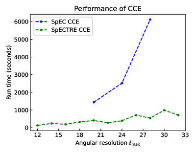
Figure 12: Performance comparison between the SpEC and SpECTRE CCE systems applied to the bouncing black hole test. We find that the SpECTRE performs considerably better for a comparable selection of simulation and stepper parameters. The non-monotonicity of the SpECTRE execution time likely arises from the dependence of the core SWSH operations performed via libsharp, and the corresponding dependence on fast Fourier transform algorithms that perform better for some mode numbers than others.

V.2 Robinson-Trautman solution

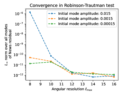
Figure 13: Residuals for the Robinson-Trautman test, computed by subtracting the extracted news from the analytic prediction of the news.

In addition to the five tests constructed previously, we have implemented an analytic test of SpECTRE CCE based on the Robinson-Trautman metric Derry et al. (1969). We specialize the construction of the Robinson-Trautman metric to the case in which there is no coordinate singularity in the asymptotic domain simulated in CCE. Unlike the tests in the above collection, the Robinson-Trautman solution both generates nontrivial asymptotic Bondi-Sachs News, and does not rely on any linearized approximations. However, it is not a fully analytic solution—a single scalar variable needs to be numerically evolved on the worldtube surface to determine the full Bondi-Sachs metric.

The specialization of the Robinson-Trautman solution that we use depends on the scalar spin-weight zero surface quantity that we denote $\omega_{\text{RT}}$. The Robinson-Trautman metric solution takes the form Derry et al. (1969),

$$ds^{2}= -\left[\left(rW+1\right)\omega_{\text{RT}}-r^{2}U\bar{U}\right](dt-dr)^{2}$$

$$-2\omega_{\text{RT}}(dt-dr)dr-2r^{2}U^{A}q_{AB}dx^{B}(dt-dr)$$

$$+r^{2}q_{AB}dx^{A}dx^{B},$$ (52)

where $q_{AB}$ represents the angular unit sphere metric, and the Bondi-Sachs scalars and angular tensors are defined in terms of the Robinson-Trautman scalar $\omega_{\text{RT}}$ as

$$W =\frac{1}{r}\left(\omega_{\text{RT}}+\eth\bar{\eth}\omega_{\text{RT}}-1\right)-\frac{2}{r^{2}\omega^{2}_{\text{RT}}},$$ (53a)

$$U \equiv U^{A}q_{A}=\frac{\eth\omega_{\text{RT}}}{r}.$$ (53b)

The Robinson-Trautman scalar may be chosen arbitrarily for a single initial retarded time $u=u_{0}$, and at all later times, is computed by integrating the evolution equation

$$\partial_{u}\omega_{\text{RT}}=-\left[\omega^{4}_{\text{RT}}\eth^{2}\bar{\eth}^{2}\omega_{\text{RT}}-\omega^{3}_{\text{RT}}\left(\eth^{2}\omega_{\text{RT}}\right)\left(\bar{\eth}^{2}\omega_{\text{RT}}\right)\right].$$ (54)

The news for the solution is

$$N=\frac{\bar{\eth}\bar{\eth}\omega_{\text{RT}}}{\omega_{\text{RT}}}.$$ (55)

We have performed the Robinson-Trautman test over a range of angular resolutions and for various initial magnitudes of the Robinson-Trautman scalar $\omega_{\text{RT}}$, and the rapid convergence for this test case is shown in Fig. 13. For our tests, we choose a starting $\omega_{\text{RT}}$ with nonzero modes:

$$a_{0\,0}=A\qquad a_{1\,-1}=4A/3\qquad a_{1\,0}=A/3(2+i)$$

$$a_{1\,1}=4A(1+2i)/3\qquad a_{2\,-2}=A(5+2i)/3,$$ (56)

where $A$ is the initial mode amplitude that is varied in Fig. 13. All other modes of $\omega_{\text{RT}}$ are zero at $t=0$.

VI Binary black hole simulation trials

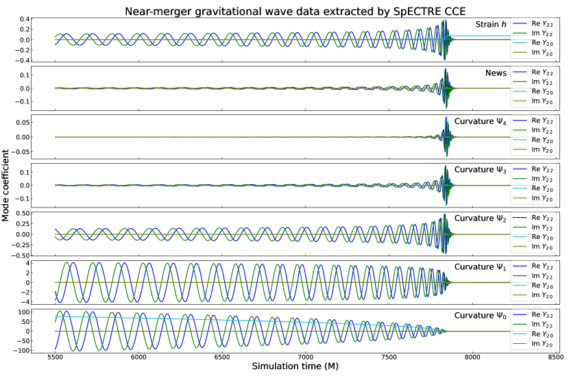
Figure 14: The last several orbits of a waveform extracted using SpECTRE CCE, generated from the $R=436$ worldtube of simulation SXS:BBH:2096.

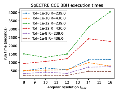
Figure 15: The runtime of SpECTRE CCE applied to the extraction of binary black hole worldtube data generated by SpEC for various stepper tolerance targets and extraction radii. In practical cases, SpECTRE CCE is able to achieve a high-precision wave extraction within 20-40 minutes of runtime.

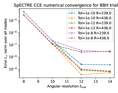
Figure 16: Convergence of the binary black hole trial execution of SpECTRE CCE, computed by comparing the extracted news to the value generated at the highest angular resolution run, $\ell_{\text{max}}=16$. The SpECTRE CCE system converges rapidly for practical use-cases.

As the capstone demonstration of the efficacy of the SpECTRE CCE system, we have performed the full wave extraction of a representative binary black hole simulation from SpEC. We have chosen the simulation SXS:BBH:2096 from the SXS catalog Boyle et al. (2019); Chu et al. (2016), for which SXS has stored worldtube data at extraction radii $R=(239,436,633,830)$.

In Fig. 14, we show the extracted $(2,2)$ and $(2,0)$ modes for each of the waveform quantities. In Fig. 16 we show the convergence in numerical resolution for each of the extraction radii, and in Fig. 15 we show the performance of the SpECTRE CCE execution for the BBH extractions. We find that SpECTRE CCE recovers the waveform and Weyl scalars to good precision, and is able to perform the wave extraction very rapidly, achieving $\sim 10^{-9}$ residuals with 20-40 minutes of runtime.

VII Upcoming improvements

VII.1 Physically motivated initial data generation

The main remaining deficit in the accuracy of the waveforms determined by SpECTRE CCE is the initial-data transient near the beginning of every characteristic evolution. Without a better method to fix the CCE data on the first hypersurface, waveform data analysis methods are typically forced to discard the first $\approx 3-5$ orbits of the resulting strain waveform, and to correct for the long-lived BMS frame shift following the initial data transient Mitman et al. (2021). The BMS shift is primarily noticeable in the strain waveform, which displays a visually apparent offset during the inspiral. Note that there are also transients (commonly called “junk radiation”) in the Cauchy evolution; those transients also force data analysis methods to discard the beginning of the waveform, but they are not as long-lived as the CCE transients and dissappear after an orbit or so.

Future work will focus on methods to generate physically motivated data for the spin-weighted scalar $\breve{J}$ and angular coordinates $x^{A}(\hat{x}^{\hat{A}})$ on the first CCE hypersurface. We anticipate that an improved initial data scheme will construct the state of the initial hypersurface as an approximation to the system in which the inspiral had proceeded arbitrarily far into the past of the first Cauchy surface. With sufficiently accurate initial data, more of the valuable Cauchy data could be recovered as high-precision waveform data, and may reduce the demands of the post-processing BMS gauge transformation.

VII.2 Cauchy-characteristic Matching

Unlike past implementations of the Cauchy-characteristic evolution system, the SpECTRE CCE module is able to operate in concert with a simultaneously running Cauchy simulation with negligible performance degradation. The key developments that allow this accomplishment are setting the CCE step size significantly larger than the Cauchy step as described in Sec. IV.2 and numerical improvements described in Sec. III.

The ability to gracefully run in tandem with a Generalized Harmonic system makes SPECTRE CCE a well-suited system for an implementation of Cauchy characteristic matching. As derived in Lindblom et al. (2006), the main piece of information that is required to determine the ingoing characteristic speeds for the generalized harmonic system is the Weyl scalar $\Psi_{0}$, computed in a choice of null tetrads associated with the Cauchy coordinates. The value of $\Psi_{0}$ can be derived directly from spectral operations on any null hypersurface in the CCE system, and transmitted to the boundary elements in the GH system to improve the physical boundary condition.

We anticipate that a successful Cauchy-characteristic matching system in SpECTRE would improve the precision of the outer boundary conditions and reduce erroneous wave reflections at the outer boundary. Further, with sufficient improvement in the boundary behavior, the outer boundary of the generalized harmonic simulation should be able to be placed at smaller radii without impacting the waveform precision. We expect, then, that a smaller simulation domain for the generalized harmonic system would enable less expensive Cauchy simulations.

VIII Conclusions

The SpECTRE CCE system represents a significant improvement over previous methods of performing CCE as well as over more traditional wave extraction methods. Our new implementation of CCE is able to rapidly extract waveforms from finished strong-field simulations or from a simultaneously running Generalized Harmonic strong-field simulation in SpECTRE. In the latter case, the SpECTRE CCE system gracefully extracts finalized waveform data in concert with the strong-field simulation. Our CCE implementation is extremely fast compared to previous implementations of CCE Winicour (1999); Bishop et al. (1997); Barkett et al. (2020), which provides significant benefits both for interoperability with other systems and in the opportunity for users to quickly iterate on new advances in waveform processing that require the use of CCE as a step in the analysis.

Our implementation takes advantage of recent advances in the understanding of the formalism underlying the system of Einstein field equations in the Bondi-Sachs and Bondi-like coordinate systems Moxon et al. (2020). As a result, the gauge is specialized to provably avoid any pure-gauge logarithms that appear in generic Bondi-Sachs-like gauges. In addition, the implementation is then able to easily compute the asymptotically leading contribution to all five Weyl scalars (see Fig. 14).

SpECTRE CCE has already begun to be used to extract valuable insights from gravitational wave data. The gains available from highly precise gravitational wave extraction and the rich data encoded in the Weyl scalars have enabled a number of valuable early investigations of waveform properties and BMS gauge transformations Mitman et al. (2020, 2021); Foucart et al. (2021); Iozzo et al. (2021b). We anticipate that precise waveform extraction will play an important role in the gravitational wave modelling pipeline as next-generation ground-based and the near future space-based gravitational wave detectors will demand extremely high quality gravitational wave models Pürrer and Haster (2020).

Appendix A World tube data representations

The worldtube metric quantities that the interior Cauchy code must supply to CCE are all components of the spatial metric $g_{ij}$, the shift $\beta^{i}$, the lapse $\alpha$, their radial derivatives $\partial_{r}g_{ij}$, $\partial_{r}\beta^{i}$, $\partial_{r}\alpha$, and their time derivatives $\partial_{t}g_{ij}$, $\partial_{t}\beta^{i}$, and $\partial_{t}\alpha$. This results in a total of 30 tensor components to store and retrieve.

However, if the initial transformation to Bondi-Sachs coordinates can be performed before storage, we need only store the boundary values of $\beta,Q,U,W,H,J,\partial_{r}J,R$, and $\partial_{u}R$. The Bondi-Sachs representation totals 14 real components. Combined with a representation in spin-weighted spherical harmonics that make good use of the relationships between $+m$ and $-m$ modes for real functions, storing Bondi-Sachs data can be a factor of 2–4 cheaper than storing the full set of metric components and their derivatives.

Because this savings is so great for large catalogs of binary black hole simulations, SpECTRE also provides a lightweight executable (ReduceCceWorldtube) for converting inefficient metric component data to the far smaller Bondi-Sachs data representation.

Appendix B Interpolation at $\mathcal{I}^{+}$

The core evolution system using the hierarchical system of CCE equations (9) gives the spin-weighted scalars $\{\breve{J},\breve{\beta},\breve{U},\breve{W},\breve{H}\}$ that determine the asymptotic partially flat Bondi-like metric (II.2). However, to determine the waveform quantities in asymptotically inertial coordinates, we must perform a final gauge transformation at $\mathcal{I}^{+}$. Because the partially flat coordinates of the evolution system ensure that the angular coordinates are asymptotically inertial—their defining equation (12) is identical to the asymptotically inertial angular coordinates constructed in Bishop et al. (1997)—we just need to perform a coordinate transformation to asymptotically inertial retarded time $\mathring{u}(\breve{u},\breve{x}^{\breve{A}})$.

The asymptotically inertial retarded time $\mathring{u}$ is determined by evolving

$$\partial_{\breve{u}}\mathring{u}=e^{2\breve{\beta}}.$$ (57)

All other coordinates are identical to their partially flat counterparts $\mathring{r}=\hat{r}$, $\mathring{\theta}=\hat{\theta}$, $\mathring{\phi}=\hat{\phi}$.

Once the asymptotically inertial retarded time $\mathring{u}$ is determined, we must perform the explicit computations of the asymptotic quantities

$$h= \breve{\bar{J}}^{(1)}+\breve{\bar{\eth}}^{2}\mathring{u}$$ (58a)

$$N= e^{-2\breve{\beta}^{(0)}}\left[\breve{\bar{H}}^{(1)}+\breve{\bar{\eth}}^{2}e^{2\breve{\beta}^{(0)}}\right]$$ (58b)

$$\Psi_{4}^{\text{Bondi}(1)}= \Psi_{4}^{\text{PF}(1)}$$ (58c)

$$\Psi_{3}^{\text{Bondi}(2)}= \Psi_{3}^{\text{PF}(2)}+\frac{1}{2}\breve{\eth}\mathring{u}\Psi_{4}^{\text{PF}(1)}$$ (58d)

$$\Psi_{2}^{\text{Bondi}(3)}= \Psi_{2}^{\text{PF}(3)}+\breve{\eth}\mathring{u}\Psi_{3}^{\text{PF}(2)}+\frac{1}{4}(\breve{\eth}\mathring{u})^{2}\Psi_{4}^{\text{PF}(1)}$$ (58e)

$$\Psi_{1}^{\text{Bondi}(4)}= \Psi_{1}^{\text{PF}(4)}+\frac{3}{2}\breve{\eth}\mathring{u}\Psi_{2}^{\text{PF}(3)}+\frac{3}{4}(\breve{\eth}\mathring{u})^{2}\Psi_{3}^{\text{PF}(2)}$$

$$+\frac{1}{8}(\breve{\eth}\mathring{u})^{3}\Psi_{4}^{\text{PF}(1)}$$ (58f)

$$\Psi_{0}^{\text{Bondi}(5)}= \Psi_{0}^{\text{PF}(5)}+2\breve{\eth}\mathring{u}\Psi_{1}^{\text{PF}(4)}+\frac{3}{4}(\breve{\eth}\mathring{u})^{2}\Psi_{2}^{\text{PF}(3)}$$

$$+\frac{1}{2}(\breve{\eth}\mathring{u})^{3}\Psi_{3}^{\text{PF}(2)}+\frac{1}{16}(\breve{\eth}\mathring{u})^{4}\Psi_{4}^{\text{PF}(1)}.$$ (58g)

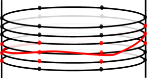
Figure 17: A sketch of the interpolation required at $\mathcal{I}^{+}$. The black rings represent the time series of spherical surface data produced by CCE at $I^{+}$ and the points represent the collocation points on which the field values are provided. The red curve represents a single value of asymptotically inertial time $\mathring{u}(\breve{u},\breve{x}^{\breve{A}})$ on which we wish to evaluate the waveform. The red points are those we would use to perform a second-order interpolation to the asymptotically inertial time. Note that we may need to use different sets of source time values $\breve{u}$ at different collocation points.

However, once we’ve computed these waveform quantities, we still need to perform the interpolation to cuts of $\mathcal{I}^{+}$ at constant inertial retarded time $\mathring{u}$. To perform the interpolation, we record several time steps of the CCE evolution, until we have sufficient data at $\mathcal{I}^{+}$ to perform a barycentric rational Floater and Hormann (2007) interpolation to the target cut of constant $\mathring{u}$. This process is illustrated in Fig. 17.

Appendix C Clenshaw recurrence details

C.0.1 Spin-weighted spherical harmonics in terms of Jacobi polynomials

A number of representation choices exist for the spin-weighted spherical harmonic basis, most of which are related by phase and sign changes. For simplicity, we take the definition of the spin-weighted spherical harmonics ${}_{s}Y_{\ell m}(\theta,\phi)$ directly in terms of the Wigner rotation matrices $d^{l}_{-m,s}(\theta)$ Goldberg et al. (1967),

$${}_{s}Y_{\ell m}(\theta,\phi)=(-1)^{m}\sqrt{\frac{2\ell+1}{4\pi}}e^{im\phi}d^{\ell}_{-m,s}(\theta)$$ (59)

The Wigner rotation matrices $d^{\ell}_{-m,s}$ may then be expressed in terms of Jacobi polynomials Varshalovich et al. (1988). Define:

$$a =|s+m|$$ (60a)

$$b =|s-m|$$ (60b)

$$k =-\frac{1}{2}(a+b)$$ (60c)

$$\lambda =\begin{cases}0,&s\geq-m,\\ s+m,&s<-m.\end{cases}$$ (60d)

Then,

$$d^{\ell}_{-m,s}(\theta)= (-1)^{\lambda}\sqrt{\frac{(\ell+k)!(\ell+k+a+b)!}{(\ell+k+a)!(\ell+k+b)!}}$$

$${}\times\sin^{a}\left(\frac{\theta}{2}\right)\cos^{b}\left(\frac{\theta}{2}\right)P^{(a,b)}_{\ell+k}(\cos\theta).$$ (61)

We have deviated from the notation of Varshalovich et al. (1988) and others by separating out the $\ell$ contribution from the variable $k$. With the notation in (C.0.1), all dependence on $\ell$ is explicit. This assists the derivation below of recurrence relations for successive $\ell$ at fixed $s$ and $m$ (and so also fixed $a$, $b$, and $k$).

Note that for any particular $(s,m)$, the lowest $\ell$-mode that is required is $\ell_{\min}=\max(|m|,|s|)$, and that $k=\min(-|m|,-|s|)$. Thus each of the recurrence relations has its lowest two contributions determined by $P_{0}^{(a,b)}$ and $P_{1}^{(a,b)}$, which have convenient closed forms:

$$P_{0}^{(a,b)}(\cos\theta) =1$$ (62a)

$$P_{1}^{(a,b)}(\cos\theta) =(a+1)+(a+b+2)\frac{\cos\theta-1}{2}$$ (62b)

For reference, the three-term recursion relation we use for the Jacobi polynomials is Bateman (1953),

$$P_{n}^{(a,b)}(x) ={}_{P}\alpha_{n}^{(a,b)}(x)P_{n-1}(x)+{}_{P}\beta_{n}^{(a,b)}P_{n-2}(x)$$ (63a)

$${}_{P}\alpha_{n}^{(a,b)}(x) =\frac{2n+b+a-1}{2n(n+a+b)}\left[(2n+a+b)x+\frac{(a^{2}-b^{2})}{2n+a+b-2}\right]$$ (63b)

$${}_{P}\beta_{n}^{(a,b)} =\frac{-(2n+a+b)(n+a-1)(n+b-1)}{n(n+a+b)(2n+a+b-2)}.$$ (63c)

In (63), we denote the recurrence coefficients with a leading subscript $P$, to avoid ambiguity with other recurrence coefficients in this paper.

C.0.2 Recursion relations for application of Clenshaw algorithm

In general, to perform a spin-weighted spherical harmonic interpolation from a prescribed set of collocation points, one first performs a transformation to spin-weighted coefficients ${}_{s}a_{\ell m}$, then interpolates to each desired $(\theta_{i},\phi_{i})$ by evaluating the sum

$$f(\theta_{i},\phi_{i})=\sum_{m=-\ell_{\max}}^{\ell_{\max}}\sum_{\ell=\min(|m|,|s|)}^{\ell_{\max}}{}_{s}a_{\ell m}\,{}_{s}Y_{\ell m}(\theta_{i},\phi_{i}).$$ (64)

The Clenshaw-based algorithm will possess an outer loop over $m\in[-\ell_{\max},\ell_{\max}]$ modes for a given spin $s$. The inner sum will then be evaluated using the Clenshaw recurrence algorithm described in section III.1. For this section, we focus on the formulas necessary to apply the Clenshaw algorithm to the innermost loop.

For spin-weighted spherical harmonics with $\ell\geq\max(|m|,|s|)+2$, we seek a recurrence relation of the form

$${}_{s}Y_{\ell m}(\theta,\phi)= {}_{Y}\alpha_{\ell}^{(a,b)}(\theta,\phi){}_{s}Y_{\ell-1\,m}(\theta,\phi)$$

$$+{}_{Y}\beta_{\ell}^{(a,b)}{}_{s}Y_{\ell-2\,m}(\theta,\phi).$$ (65)

The coefficients in (C.0.2) are labeled with a leading subscript $Y$, and may be inferred from the relation between the spin-weighted spherical harmonics and the Jacobi polynomials. The result is the recurrence coefficients

$${}_{Y}\alpha_{\ell}^{(a,b)}= \sqrt{\frac{2\ell+1}{2\ell-1}}\sqrt{\frac{(\ell+k)(\ell+k+a+b)}{(\ell+k+a)(\ell+k+b)}}\,{}_{P}\alpha_{\ell+k}^{(a,b)}(\cos\theta)$$

$$= \sqrt{\frac{2\ell+1}{2\ell-1}}\frac{2(\ell+k)+b+a-1}{2\sqrt{(\ell+k)(\ell+k+a+b)(\ell+k+a)(\ell+k+b)}}$$

$$\times\left[(2(\ell+k)+a+b)\cos\theta+\frac{a^{2}-b^{2}}{2(\ell+k)+a+b-2}\right],$$ (66a)

$${}_{Y}\beta_{\ell}^{(a,b)}= \sqrt{\frac{2\ell+1}{2\ell-3}}\sqrt{\frac{(\ell+k)(\ell+k-1)(\ell+k+a+b)(\ell+k+a+b-1)}{(\ell+k+a)(\ell+k+a-1)(\ell+k+b)(\ell+k+b-1)}}\,{}_{P}\beta_{\ell+k}^{(a,b)}$$

$$= -\sqrt{\frac{(2\ell+1)(\ell+k+a-1)(\ell+k+b-1)(\ell+k-1)(\ell+k+a+b-1)}{(2\ell-3)(\ell+k)(\ell+k+a+b)(\ell+k+a)(\ell+k+b)}}\frac{2(\ell+k)+a+b}{2(\ell+k)+a+b-2}.$$ (66b)

When generating the ${}_{Y}\alpha$ and ${}_{Y}\beta$ coefficients, it would be wasteful to populate a full two-dimensional space of integers for $(a,b)$ values. For each spin $s$, there is a one-to-one mapping between $m$ and $(a,b)$ pairs, so for each spin value, exactly $2\ell_{\max}+1$ recurrence coefficient sets should be generated. For each coefficient set, coefficients are needed with indices $\ell\in[\min(|m|,|s|),\ell_{\max}]$.

C.0.3 Relations between successive iterations for spin-weighted spherical harmonics

In this section, we describe the computations necessary to obtain the two lowest spin-weighted spherical harmonics for each Clenshaw recurrence evaluation, and suggest a method by which several of these explicit functions may also be determined by recurrence in $m$ to limit evaluations of the factorial prefactor and powers of trigonometric functions found in (C.0.1).

First, we note that it is desirable to first evaluate the recurrence for $m=0$, then perform the sequence of positive $m$ and negative $m$ as further branches. The reason for this evaluation structure is based on the observation that successive factors of $\sin^{a}(\theta/2)\cos^{b}(\theta/2)$ can be computed from previous ones provided that $a$ and $b$ both increment from one step to the next. From (24), we see that that this will be true for ascending values of $|m|$ whenever $|s|<|m|$.

Therefore, it is possible to recursively obtain ${}_{s}Y_{|m|\,m}$ and ${}_{s}Y_{|m|+1\,m}$ from the previously determined harmonics, for all harmonics where $|m|>|s|$. Recursive construction won’t be available for complete generality, as the steps for which $|s|\geq|m|$ involve both the increase and decrease of $a$’s and $b$’s, so would involve the potentially dangerous division by $\sin(\theta/2)$, which is ill-defined near one pole. For those $2|s|$ steps, our algorithm accepts the cost of the direct evaluation of the (small) powers. For most realistic applications, the value $|s|$ will be far smaller than $\ell_{\max}$, so most $m$ steps can be evaluated by the recursive method.

In particular, for $|m|>|s|$, the first required explicit function for the Clenshaw recurrence is

$${}_{s}Y_{|m|\,m}=(-1)^{\Delta\lambda}\sqrt{\frac{2|m|+1}{2|m|-1}\frac{(\ell+k+a+b-1)(\ell+k+a+b)}{(\ell+k+a)(\ell+k+b)}}e^{i\phi}\sin\left(\theta/2\right)\cos\left(\theta/2\right)\begin{cases}{}_{s}Y_{|m|-1\,m-1},&m>0,\\ {}_{s}Y_{|m|-1\,m+1},&m<0,\end{cases}$$ (67)

where the difference $\Delta\lambda=\lambda_{m}-\lambda_{\pm m}$ is sufficiently cheap to compute on a case-by-case basis. Finally, the second harmonic can always be easily evaluated from the first harmonic of a sequence. The simple relation arises from noting that the first Jacobi polynomial in each sequence is unity. Therefore, computation can once again be saved in determining ${}_{s}Y_{\ell_{\min}+1,m}$:

$${}_{s}Y_{\ell_{\min}+1\,m}=\sqrt{\frac{2\ell_{\min}+3}{2\ell_{\min}+1}}\sqrt{\frac{(\ell_{\min}+k+1)(\ell_{\min}+k+a+b+1)}{(\ell_{\min}+k+a+1)(\ell_{\min}+k+b+1)}}\left[(a+1)+(a+b+2)\frac{(\cos\theta-1)}{2}\right]{}_{s}Y_{\ell_{\min}\,m}.$$ (68)

With the above recurrence for the successive starting $m$ modes, it is only necessary to evaluate ${}_{s}Y_{\ell_{\min}\,m}$ for $|m|\leq|s|$ from the explicit formulas for the Wigner rotation matrices (C.0.1).

References

- Abbott et al. (2016a) B. P. Abbott et al. (LIGO Scientific, Virgo), Phys. Rev. Lett. 116, 061102 (2016a), arXiv:1602.03837 [gr-qc] .
- Abbott et al. (2016b) B. P. Abbott et al. (LIGO Scientific, Virgo), Phys. Rev. Lett. 116, 241103 (2016b), arXiv:1606.04855 [gr-qc] .
- Abbott et al. (2019) B. P. Abbott et al. (LIGO Scientific, Virgo), Phys. Rev. X9, 031040 (2019), arXiv:1811.12907 [astro-ph.HE] .
- Abbott et al. (2018) B. P. Abbott et al. (KAGRA, LIGO Scientific, VIRGO), Living Rev. Rel. 21, 3 (2018), arXiv:1304.0670 [gr-qc] .
- Hanna (2010) C. Hanna (LIGO Scientific, Virgo), Numerical relativity and data analysis. Proceedings, 3rd Annual Meeting, NRDA 2009, Potsdam, Germany, July 6-9, 2009, Class. Quant. Grav. 27, 114003 (2010).
- Flanagan and Hughes (1998) E. E. Flanagan and S. A. Hughes, Phys. Rev. D57, 4535 (1998), arXiv:gr-qc/9701039 [gr-qc] .
- Abbott et al. (2016c) B. P. Abbott et al. (LIGO Scientific, Virgo), Phys. Rev. D94, 064035 (2016c), arXiv:1606.01262 [gr-qc] .
- Kumar et al. (2019) P. Kumar, J. Blackman, S. E. Field, M. Scheel, C. R. Galley, M. Boyle, L. E. Kidder, H. P. Pfeiffer, B. Szilagyi, and S. A. Teukolsky, Phys. Rev. D99, 124005 (2019), arXiv:1808.08004 [gr-qc] .
- Kumar et al. (2015) P. Kumar, K. Barkett, S. Bhagwat, N. Afshari, D. A. Brown, G. Lovelace, M. A. Scheel, and B. Szilágyi, Phys. Rev. D92, 102001 (2015), arXiv:1507.00103 [gr-qc] .
- Lange et al. (2017) J. Lange et al., Phys. Rev. D96, 104041 (2017), arXiv:1705.09833 [gr-qc] .
- Lovelace et al. (2016) G. Lovelace et al., Class. Quant. Grav. 33, 244002 (2016), arXiv:1607.05377 [gr-qc] .
- Pürrer and Haster (2020) M. Pürrer and C.-J. Haster, Phys. Rev. Res. 2, 023151 (2020), arXiv:1912.10055 [gr-qc] .
- Fritschel et al. (2020) P. Fritschel et al. (LIGO Scientific Collaboration), Instrument Science White Paper 2020, Tech. Rep. (2020).
- Nguyen (2021) C. Nguyen (Virgo), in 16th Rencontres du Vietnam: Theory meeting experiment: Particle Astrophysics and Cosmology (2021) arXiv:2105.09247 [astro-ph.IM] .
- Reitze et al. (2019) D. Reitze et al., Cosmic explorer: The u.s. contribution to gravitational-wave astronomy beyond ligo (2019), arXiv:1907.04833 [astro-ph.IM] .
- Maggiore et al. (2020) M. Maggiore, C. V. D. Broeck, N. Bartolo, E. Belgacem, D. Bertacca, M. A. Bizouard, M. Branchesi, S. Clesse, S. Foffa, J. García-Bellido, and et al., Journal of Cosmology and Astroparticle Physics 2020 (03), 050–050.
- Amaro-Seoane et al. (2017) P. Amaro-Seoane et al., Laser interferometer space antenna (2017), arXiv:1702.00786 [astro-ph.IM] .
- Luo et al. (2016) J. Luo, L.-S. Chen, H.-Z. Duan, Y.-G. Gong, S. Hu, J. Ji, Q. Liu, J. Mei, V. Milyukov, M. Sazhin, and et al., Classical and Quantum Gravity 33, 035010 (2016).
- Sato et al. (2017) S. Sato et al., Journal of Physics: Conference Series 840, 012010 (2017).
- SpE (a) The Spectral Einstein Code, https://black-holes.org/code/spec.html (a), accessed: 2021-07-16.
- Loffler et al. (2012) F. Loffler et al., Class. Quant. Grav. 29, 115001 (2012), arXiv:1111.3344 [gr-qc] .
- Bruegmann et al. (2004) B. Bruegmann, W. Tichy, and N. Jansen, Phys. Rev. Lett. 92, 211101 (2004), arXiv:gr-qc/0312112 .
- Ruchlin and Etienne (2018) I. Ruchlin and T. W. Etienne, Zachariah B.and Baumgarte, Phys. Rev. 97, 064036 (2018), arXiv:1712.07658 [gr-qc] .
- Iozzo et al. (2021a) D. A. B. Iozzo, M. Boyle, N. Deppe, J. Moxon, M. A. Scheel, L. E. Kidder, H. P. Pfeiffer, and S. A. Teukolsky, Phys. Rev. D 103, 024039 (2021a), arXiv:2010.15200 [gr-qc] .
- Bishop and Rezzolla (2016) N. T. Bishop and L. Rezzolla, Living Rev. Rel. 19, 2 (2016), arXiv:1606.02532 [gr-qc] .
- Boyle et al. (2019) M. Boyle et al., Class. Quant. Grav. 36, 195006 (2019), arXiv:1904.04831 [gr-qc] .
- Healy et al. (2019) J. Healy, C. O. Lousto, J. Lange, R. O’Shaughnessy, Y. Zlochower, and M. Campanelli, Phys. Rev. D 100, 024021 (2019), arXiv:1901.02553 [gr-qc] .
- Jani et al. (2016) K. Jani, J. Healy, J. A. Clark, L. London, P. Laguna, and D. Shoemaker, Class. Quant. Grav. 33, 204001 (2016), arXiv:1605.03204 [gr-qc] .
- Mitman et al. (2020) K. Mitman, J. Moxon, M. A. Scheel, S. A. Teukolsky, M. Boyle, N. Deppe, L. E. Kidder, and W. Throwe, Phys. Rev. D 102, 104007 (2020), arXiv:2007.11562 [gr-qc] .
- Bishop et al. (1996) N. T. Bishop, R. Gomez, L. Lehner, and J. Winicour, Phys. Rev. D 54, 6153 (1996), arXiv:gr-qc/9705033 .
- Winicour (2012) J. Winicour, Living Rev. Rel. 15, 2 (2012).
- Babiuc et al. (2011) M. C. Babiuc, J. Winicour, and Y. Zlochower, Class. Quant. Grav. 28, 134006 (2011), arXiv:1106.4841 [gr-qc] .
- Winicour (1999) J. Winicour, AIP Conf. Proc. 493, 35 (1999).
- Bishop et al. (1997) N. T. Bishop, R. Gomez, L. Lehner, M. Maharaj, and J. Winicour, Phys. Rev. D 56, 6298 (1997), arXiv:gr-qc/9708065 .
- Barkett et al. (2020) K. Barkett, J. Moxon, M. A. Scheel, and B. Szilágyi, Phys. Rev. D 102, 024004 (2020), arXiv:1910.09677 [gr-qc] .
- Handmer and Szilagyi (2015) C. J. Handmer and B. Szilagyi, Class. Quant. Grav. 32, 025008 (2015), arXiv:1406.7029 [gr-qc] .
- Handmer et al. (2015) C. J. Handmer, B. Szilágyi, and J. Winicour, Class. Quant. Grav. 32, 235018 (2015), arXiv:1502.06987 [gr-qc] .
- Handmer et al. (2016) C. J. Handmer, B. Szilágyi, and J. Winicour, Class. Quant. Grav. 33, 225007 (2016), arXiv:1605.04332 [gr-qc] .
- Deppe et al. (2021) N. Deppe, W. Throwe, L. E. Kidder, N. L. Fischer, F. Hébert, J. Moxon, C. Armaza, G. S. Bonilla, P. Kumar, G. Lovelace, E. O’Shea, H. P. Pfeiffer, M. A. Scheel, S. A. Teukolsky, I. Anantpurkar, M. Boyle, F. Foucart, M. Giesler, J. S. Guo, D. A. B. Iozzo, Y. Kim, I. Legred, D. Li, A. Macedo, D. Melchor, M. Morales, K. C. Nelli, T. Ramirez, H. R. Rüter, J. Sanchez, S. Thomas, N. A. Wittek, and T. Wlodarczyk, SpECTRE (2021).
- Moxon et al. (2020) J. Moxon, M. A. Scheel, and S. A. Teukolsky, Phys. Rev. D 102, 044052 (2020), arXiv:2007.01339 [gr-qc] .
- Kidder et al. (2017) L. E. Kidder et al., J. Comput. Phys. 335, 84 (2017), arXiv:1609.00098 [astro-ph.HE] .
- Kalé and Krishnan (1993) L. Kalé and S. Krishnan, in Proceedings of OOPSLA’93, edited by A. Paepcke (ACM Press, 1993) pp. 91–108.
- Kale and Bhatele (2013) L. V. Kale and A. Bhatele, eds., Parallel Science and Engineering Applications: The Charm++ Approach (Taylor & Francis Group, CRC Press, 2013).
- (44) Charm++, https://charm.cs.illinois.edu/research/charm, accessed: 2021-07-16.
- SpE (b) SpECTRE github page, https://github.com/sxs-collaboration/spectre (b), accessed: 2021-07-16.
- SpE (c) SpECTRE documentation page, https://spectre-code.org/ (c), accessed: 2021-07-16.
- SpE (d) SpECTRE CCE tutorial page, https://spectre-code.org/tutorial_cce.html (d), accessed: 2021-07-16.
- Bishop et al. (1998) N. T. Bishop, R. Gomez, L. Lehner, B. Szilagyi, J. Winicour, and R. A. Isaacson, Cauchy characteristic matching, in Black Holes, Gravitational Radiation and the Universe: Essays in Honor of C.V. Vishveshwara, edited by B. R. Iyer and B. Bhawal (1998) arXiv:gr-qc/9801070 .
- Reinecke and Seljebotn (2013) M. Reinecke and D. S. Seljebotn, Astronomy & Astrophysics 554, A112 (2013).
- Lib (a) libsharp, https://github.com/Libsharp/libsharp (a), accessed: 2021-08-25.
- Bishop et al. (2011) N. Bishop, D. Pollney, and C. Reisswig, Class. Quant. Grav. 28, 155019 (2011), arXiv:1101.5492 [gr-qc] .
- York (1999) J. W. York, Jr., Phys. Rev. Lett. 82, 1350 (1999), arXiv:gr-qc/9810051 .
- Pfeiffer and York (2003) H. P. Pfeiffer and J. W. York, Jr., Phys. Rev. D 67, 044022 (2003), arXiv:gr-qc/0207095 .
- Mitman et al. (2021) K. Mitman et al., Phys. Rev. D 104, 024051 (2021), arXiv:2105.02300 [gr-qc] .
- (55) blaze, https://bitbucket.org/blaze-lib/blaze/src/master/, accessed: 2021-08-02.
- Press et al. (2007) W. H. Press, S. A. Teukolsky, W. T. Vetterling, and B. P. Flannery, Numerical Recipes (Cambridge University Press, 2007).
- Lib (b) libxsmm, https://github.com/hfp/libxsmm (b), accessed: 2021-08-25.
- Lindblom et al. (2006) L. Lindblom, M. A. Scheel, L. E. Kidder, R. Owen, and O. Rinne, Class. Quant. Grav. 23, S447 (2006), arXiv:gr-qc/0512093 .
- Harier et al. (1993) E. Harier, S. P. Nørsett, and G. Wanner, Solving Ordinary Differential Equations I (Springer, 1993).
- Throwe and Teukolsky (2020) W. Throwe and S. A. Teukolsky, A high-order, conservative integrator with local time-stepping (2020), arXiv:1811.02499 [math.NA] .
- Floater and Hormann (2007) M. S. Floater and K. Hormann, Numer. Math. 107, 315 (2007).
- Bishop (2005) N. T. Bishop, Class. Quant. Grav. 22, 2393 (2005), arXiv:gr-qc/0412006 .
- Teukolsky (1982) S. A. Teukolsky, Phys. Rev. D 26, 745 (1982).
- Derry et al. (1969) L. Derry, R. Isaacson, and J. Winicour, Phys. Rev. 185, 1647 (1969).
- Chu et al. (2016) T. Chu, H. Fong, P. Kumar, H. P. Pfeiffer, M. Boyle, D. A. Hemberger, L. E. Kidder, M. A. Scheel, and B. Szilagyi, Class. Quant. Grav. 33, 165001 (2016), arXiv:1512.06800 [gr-qc] .
- Foucart et al. (2021) F. Foucart et al., Phys. Rev. D 103, 064007 (2021), arXiv:2010.14518 [gr-qc] .
- Iozzo et al. (2021b) D. A. B. Iozzo et al., Phys. Rev. D 103, 124029 (2021b), arXiv:2104.07052 [gr-qc] .
- Goldberg et al. (1967) J. N. Goldberg, A. J. MacFarlane, E. T. Newman, F. Rohrlich, and E. C. G. Sudarshan, J. Math. Phys. 8, 2155 (1967).
- Varshalovich et al. (1988) D. A. Varshalovich, A. N. Moskalev, and V. K. Khersonsky, Spherical harmonics, in Quantum Theory of Angular Momentum (World Scientific, Singapore, 1988) Chap. 5, pp. 130–169.
- Bateman (1953) H. Bateman, Higher Transcendental functions, vol. II, the Bateman Manuscript Project, edited by A. Erdélyi, W. Magnus, F. OberHettinger, and F. G. Tricomi (McGraw-Hill, 1953).