Sampling based Computation of Viability Domain to
Prevent Safety Violations by Attackers

Abstract

This paper studies the security of cyber-physical systems under attacks. Our goal is to design system parameters, such as a set of initial conditions and input bounds so that it is secure by design. To this end, we propose new sufficient conditions to guarantee the safety of a system under adversarial actuator attacks. Using these conditions, we propose a computationally efficient sampling-based method to verify whether a set is a viability domain for a general class of nonlinear systems. In particular, we devise a method of checking a modified barrier function condition on a finite set of points to assess whether a set can be rendered forward invariant. Then, we propose an iterative algorithm to compute the set of initial conditions and input constraint set to limit what an adversary can do if it compromises the vulnerable inputs. Finally, we utilize a Quadratic Program approach for online control synthesis.

I Introduction

Security has become one of the most critical problems in the field of Cyber-Physical Systems (CPS), as illustrated by several incidents of attacks that happened in the past few years [1, 2]. There are two types of security mechanisms for protecting CPS [3] i) proactive, which considers design choices deployed in the CPS before attacks, and ii) reactive, which take effect after an attack is detected.

While reactive methods are less conservative than proactive mechanisms, they heavily rely on fast and accurate attack detection mechanisms. Although there is a plethora of work on attack detection for CPS [4, 5], it is generally possible to design a stealthy attack such that the system behavior remains close to its expected behavior, thus evading attack-detection solutions [6]. Intrusion detection systems also produce a large number of false positives, which can lead to a large operational overhead of security analysts dealing with irrelevant alerts [7]. On the other hand, a proactive method can be more effective in practice, particularly against stealthy attacks. Attacks on a CPS can disrupt the natural operation of the system. One of the most desirable system properties is safety, i.e., the system does not go out of a safe zone. Safety is an essential requirement, violation of which can result in failure of the system, loss of money, or even loss of human life, particularly when a system is under attack [8].

In most practical problems, safety can be realized as guaranteeing forward-invariance of a safe set. Control barrier function (CBF) based approach [9] to guarantee forward invariance of the safe region has become very popular in the last few years since a safe control input can be efficiently computed using a Quadratic Program (QP) with CBF condition as the constraint. Most of the prior work on safety using CBFs, e.g., [9], assumes that the viability domain, i.e., the set of initial conditions from which forward invariance of the safe set can be guaranteed, is known. In practice, it is not an easy task to compute the viability domain for a nonlinear control system. Optimization-based methods, such as Sum-of-Squares (SOS) techniques, have been used in the past to compute this domain (see [10]). However, SOS-based approaches are only applicable to systems whose dynamics is given by polynomial functions, thus limiting their applications. Another method popularly used in the literature for computing the viability domain is Hamilton-Jacobi (HJ) based reachability analysis, see, e.g., [11]. However, such an analysis is computationally expensive, particularly for higher dimensional systems. We propose a novel sampling-based method to compute the viability domain for a general class of nonlinear control systems to overcome these limitations.

In this work, we consider a general class of nonlinear systems under actuator attacks and propose a method of computing a set of initial conditions and an input constraint set such that the system remains secure by design. In particular, we consider actuator manipulation, where an attacker can assign arbitrary values to the input signals for a subset of the actuators in a given bound. We consider the property of safety with respect to an unsafe set and propose sufficient conditions using sampling of the boundary of a set to verify whether the set is a viability domain under attacks. Using these conditions, we propose a computationally tractable algorithm to compute the set of initial conditions and the input constraint set such that the system’s safety can be guaranteed under attacks. In effect, our proposed method results in a secure-by-design system that is resilient against actuator attacks. Finally, we leverage these sets in a QP-based approach with provable feasibility for real-time online feedback synthesis. The contributions of the paper are summarized below:

• We present sampling-based sufficient conditions to assess whether a given set can be rendered forward invariant for a general class of nonlinear system. To the best of the authors’ knowledge, this is the first work utilizing sampled-data approach for computing a viability domain;

• We present a novel iterative algorithm to compute a viability domain and an input constraint set to guarantee system safety under attacks. Unlike [10, 11], the proposed method is applicable for general nonlinear control systems and is scalable with the system dimension.

Notation: Throughout the paper, $\mathbb{R}$ denotes the set of real numbers and $\mathbb{R}_{+}$ denotes the set of non-negative real numbers. We use $|x|$ to denote the Euclidean norm of a vector $x\in\mathbb{R}^{n}$. We use $\partial S$ to denote the boundary of a closed set $S\subset\mathbb{R}^{n}$ and $\textrm{int}(S)$ to denote its interior and $|x|_{S}=\inf_{y\in S}|x-y|$, to denote the distance of $x\in\mathbb{R}^{n}$ from the set $S$. The Lie derivative of a continuously differentiable function $h:\mathbb{R}^{n}\rightarrow\mathbb{R}$ along a vector field $f:\mathbb{R}^{n}\rightarrow\mathbb{R}^{m}$ at a point $x\in\mathbb{R}^{n}$ is denoted as $L_{f}h(x)\coloneqq\frac{\partial h}{\partial x}(x)f(x)$.

II Problem formulation

We start with defining a model for the system and the attacker considered in this paper.

II-A System model

Consider a nonlinear control system $\mathcal{S}$ given as

$$\mathcal{S}:\begin{cases}\dot{x}=F(x,u)+d(t,x),\\ x\in\mathcal{D},u\in\mathcal{U},\end{cases}$$ (1)

where $F:\mathcal{D}\times\mathcal{U}\to\mathbb{R}^{n}$ is a known function continuous on $:\mathcal{D}\times\mathcal{U}$, with $\mathcal{D}\subset\mathbb{R}^{n}$ and $\mathcal{U}\subset\mathbb{R}^{m}$, $d:\mathbb{R}_{+}\times\mathbb{R}^{n}\rightarrow\mathbb{R}^{n}$ is unknown and represents the unmodeled dynamics, $x\in\mathcal{D}$ is the system state, and $u\in\mathcal{U}$ is the control input.

II-B Attacker model

In this paper, we consider attacks on the control input of the system. In particular, we consider an attack where a subset of the components of the control input is compromised. Under such an attack, the system input takes the form:

$$u=(u_{v},u_{s}),$$ (2)

where $u_{v}\in\mathcal{U}_{v}\subset\mathbb{R}^{m_{v}}$ represents the vulnerable components of the control input that might be compromised or attacked, and $u_{s}\in\mathcal{U}_{s}\subset\mathbb{R}^{m_{s}}$ the secure part that cannot be attacked, with $m_{v}+m_{s}=m$ and $\mathcal{U}\coloneqq\mathcal{U}_{v}\times\mathcal{U}_{s}$. Under this class of attack, we assume that we know which components of the control input are vulnerable. For example, if the system has four inputs so that $u=\begin{bmatrix}u_{1}&u_{2}&u_{3}&u_{4}\end{bmatrix}^{T}$, and $u_{1},u_{3}$ can be attacked, then we assume that this information is known, and $u_{v}$ is comprised of $u_{1}$ and $u_{3}$. We discuss how to address the assumption of which components of the control input are vulnerable in Remark 1 in Section IV.

Such attack models have been used in prior work, see e.g., [12], and can be implemented in practice by designing the dynamic range of the actuator to preserve its bounds. It can also be implemented in software with the help of a reference monitor [13] between the controller and the actuator that can check if the desired control inputs satisfy the security policy [12]. As discussed in [14], various prototypical attacks, such as stealth attacks, replay attacks, and false-data injection attacks can be captured by the attack model in (2). In addition to representing a real-world scenario where system actuators have physical limits, constraining the vulnerable control input $u_{v}$ in the set $\mathcal{U}_{v}$ has several advantages:

• It restricts how much an attacker can change the nominal operation of the system [15], and can be implemented physically, so an attacker cannot bypass it.

• It can be utilized to design a detection mechanism, e.g., if $u_{v}\notin\mathcal{U}_{v}$, a flag can be raised signifying that the system is under an attack. Schemes that raise a threshold-based flag are commonly used as detection mechanism [5].

• The constraint set $\mathcal{U}_{v}$ can be designed appropriately such that the system remains secured under attacks, as discussed in Section IV (see also [12, 15]).

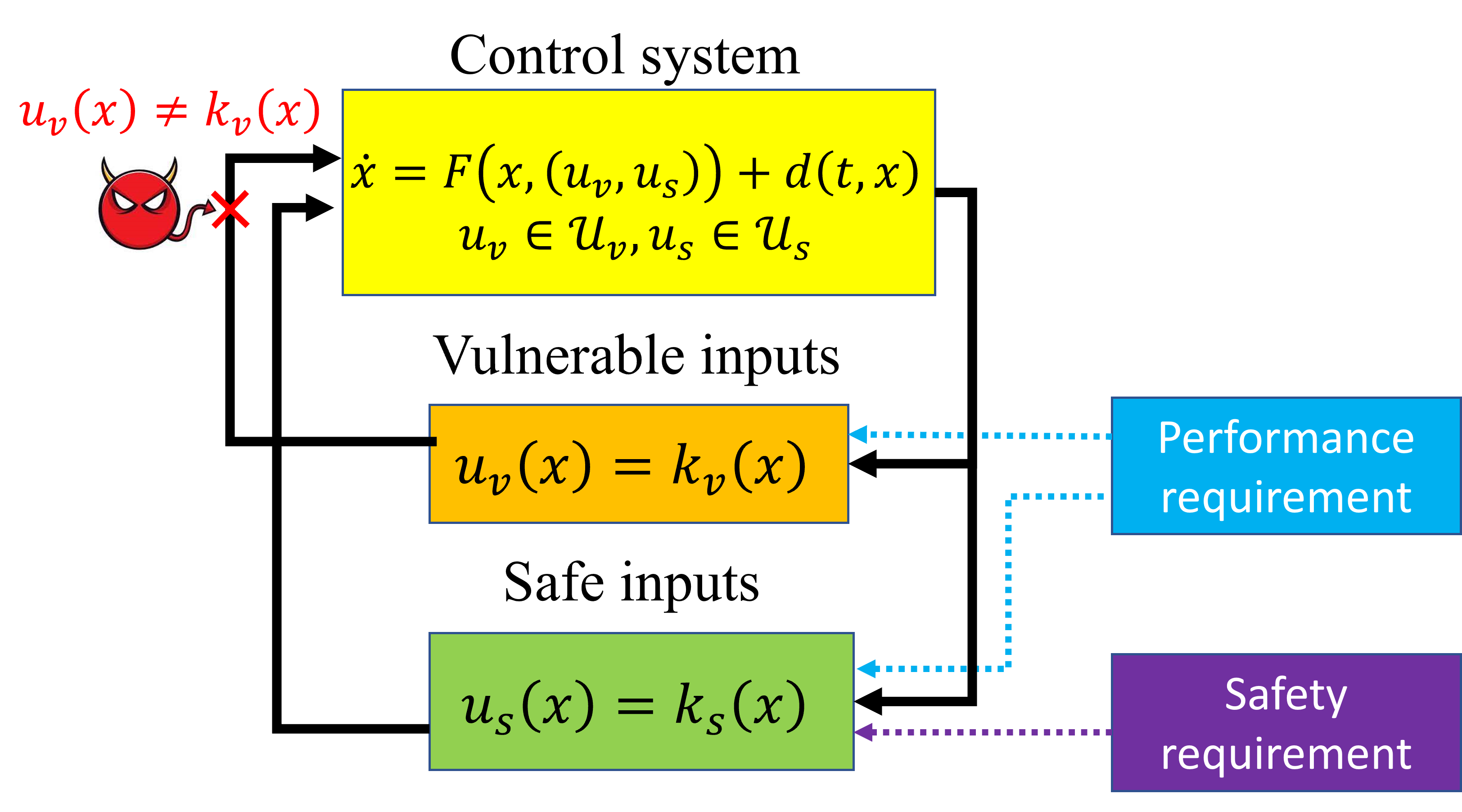
Figure 1: Overview of our approach.

Now, we present the control design objectives. Consider a non-empty, compact set $S\subset\mathbb{R}^{n}$, referred to as safe set, to be rendered forward invariant. We make the following assumption on the unmodeled dynamics $d$ in (1):

Assumption 1.

There exists $\delta>0$ such that $|d(t,x)|\leq\delta$ for all $t\geq 0$ and $x\in\mathcal{D}$.

We consider two properties when designing the control law, an essential property (safety), imposed while designing the secure input $u_{s}$, and a desirable property (performance), imposed while designing both $u_{s}$ and $u_{v}$ (see Figure 1). The problem we study in this paper is as follows.

Problem 1.

Given the system in (1) with unmodeled dynamics $d$ that satisfies Assumption 1, a set $S$ and the attack model in (2), design a feedback law $k_{s}:\mathbb{R}^{n}\rightarrow\mathcal{U}_{s}$, and find a set of initial conditions $X_{0}\subset S$ and the input constraint set $\tilde{\mathcal{U}}_{v}\subset\mathcal{U}_{v}$, such that for all $x(0)\in X_{0}$ and $u_{v}:\mathbb{R}_{+}\rightarrow\tilde{\mathcal{U}}_{v}$, the closed-loop trajectories $x:\mathbb{R}_{+}\rightarrow\mathbb{R}^{n}$ of (1) resulting from using $u_{s}=k_{s}(x)$ satisfy $x(t)\in S$ for all $t\geq 0$.

In plain words, we consider the problem of designing a feedback law $u_{s}$ and compute a set of initial conditions $X_{0}$ and input constraint set $\tilde{\mathcal{U}}_{v}$, such that even under an attack as per the attack model (2), the system trajectories do not leave the safe set $S$, i.e., the system is secure by design. In this work, we assume that the safe set is given as $S\coloneqq\{x\;|\;B(x)\leq 0\}$ where $B:\mathbb{R}^{n}\rightarrow\mathbb{R}$ is a sufficiently smooth user-defined function.

II-C Outline of approach

Given a control system (1), and an attack model (2), we first identify a safe set $S\subset\mathbb{R}^{n}$ and the vulnerable input $u_{v}$. Then, our approach to solving Problem 1 involves the following steps (see Figure 2):

• Establish the existence of $X_{0}$ and $\mathcal{U}_{v}$ (Section III): leverage CBFs to find sufficient conditions to check whether there exist a set of initial conditions $X_{0}$, input constraint set $\tilde{\mathcal{U}}_{v}\subset\mathcal{U}_{v}$, and a control input $u_{s}$ for all $x\in X_{0}$ that can solve Problem 1;

• Numerical method for computation of $X_{0}$ and $\mathcal{U}_{v}$ (Section IV): use conditions in step 1) to formulate a numerical method for computing sets $X_{0}$ and $\tilde{\mathcal{U}}_{v}$;

• Feedback law synthesis (Section V): use the sets $X_{0}$ and $\tilde{\mathcal{U}}_{v}$ from step 2) to design a feedback control law $u_{s}=k_{s}(x)$ that solves Problem 1.

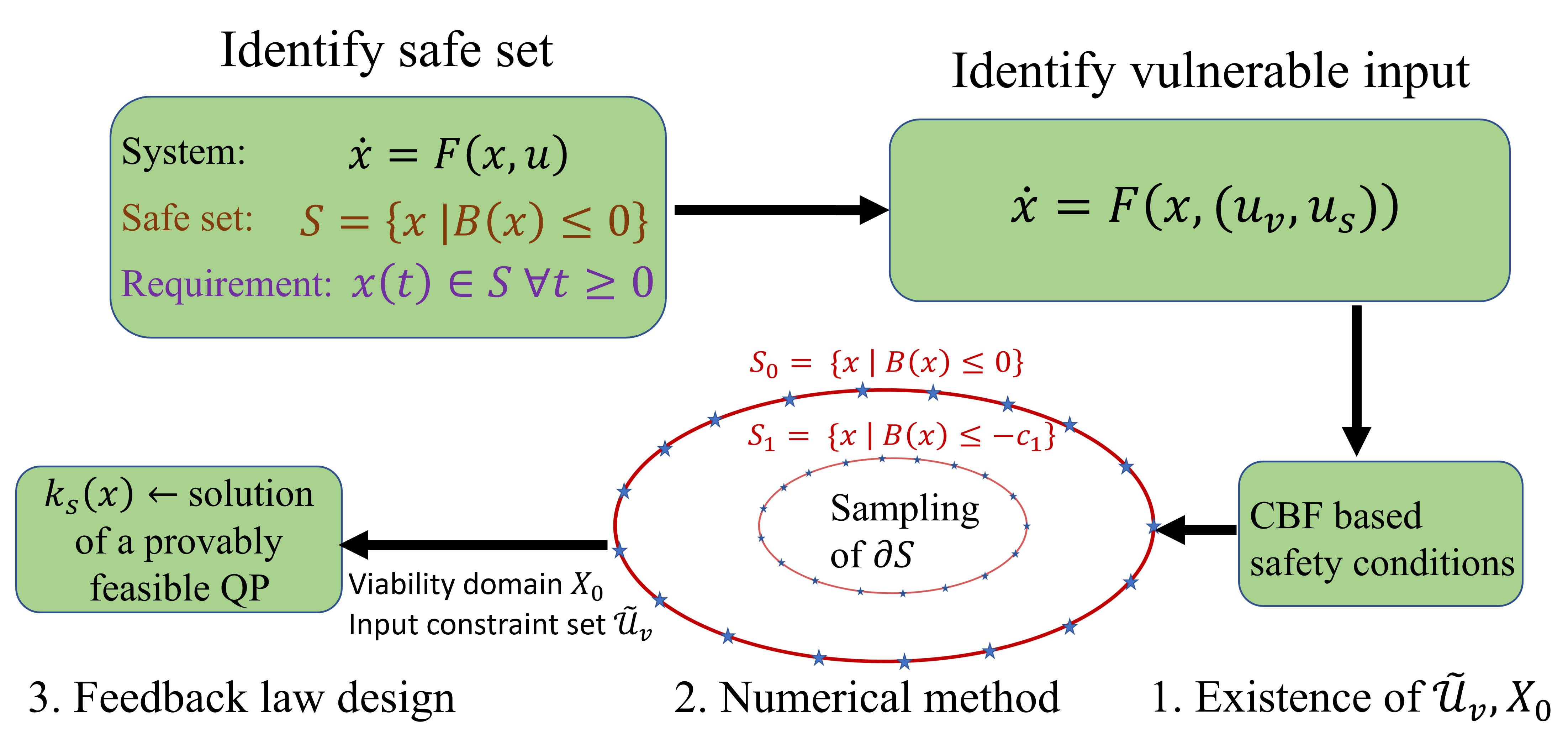
Figure 2: Approach for safe feedback design under attacks.

II-D Preliminaries

Next, we present preliminaries on forward invariance.

Definition 1.

A set $S\subset\mathbb{R}^{n}$ is termed as forward invariant for system (1) if every solution $x:\mathbb{R}_{+}\rightarrow\mathbb{R}^{n}$ of (1) satisfies $x(t)\in S$ for all $t\geq 0$ and for all initial conditions $x(0)\in S$.

Next, we review a sufficient condition for guaranteeing forward invariance of a set in the absence of an attack. For the sake of simplicity, in what follows, we assume that every solution of (1) exists and is unique in forward time for all $t\geq 0$ whether or not there is an attack on the system.

Lemma 1 ([17]).

Given a continuously differentiable function $B:\mathbb{R}^{n}\rightarrow\mathbb{R}$, the set $S=\{x\;|\;B(x)\leq 0\}$ is forward invariant for (1) with $d\equiv 0$ if the following condition holds:

$$\inf_{u\in\mathcal{U}}L_{F}B(x,u)\leq 0\quad\forall x\in\partial S.$$ (3)

Satisfaction of (3) means the set $S$ is termed as a viability domain for system (1) with $d\equiv 0$. Using Lemma 1, and following the notion of robust CBF in [18], we can state the following result guaranteeing forward invariance in the presence of disturbance $d$.

Lemma 2 ([18]).

Given a continuously differentiable function $B:\mathbb{R}^{n}\rightarrow\mathbb{R}$, the set $S=\{x\;|\;B(x)\leq 0\}$ is forward invariant for (1) under $d$ satisfying Assumption 1 if the following condition holds:

$$\inf_{u\in\mathcal{U}}L_{F}B(x,u)\leq-l_{B}\delta\quad\forall x\in\partial S,$$ (4)

where $l_{B}$ is the Lipschitz constant of the function $B$.

III Sufficient conditions for safety

In this section, we present sufficient conditions that guarantee the security of the system model (1) against attacks on the input. We say that the system (1) is secure with respect to the safety property for a set $S$ if for all initial conditions $x(0)\in S$, $x(t)\in S$ for all $t\geq 0$, $u_{v}\in\mathcal{U}_{v}$ and $d$ satisfying Assumption 1. Given $B$ and $F$, define $H:\mathbb{R}^{n}\times\mathbb{R}^{m_{v}}\rightarrow\mathbb{R}$:

$$H(x,u_{v})\coloneqq\inf_{u_{s}\in\mathcal{U}_{s}}L_{F}B(x,(u_{v},u_{s})).$$ (5)

It is not necessary that the zero sublevel set $S$ of the function $B$ is a viability domain for system (1). Any non-empty sublevel set $S_{c}\coloneqq\{x\;|\;B(x)\leq-c\}$, where $c\geq 0$, being a viability domain is sufficient for safety of the system. Note that the set $S_{c}$ is non-empty for $0\leq c\leq-\min\limits_{x\in S}B(x)$. Define $c_{M}\in\mathbb{R}$ as

$$c_{M}\coloneqq-\min\limits_{x\in S}B(x),$$ (6)

so that the set of feasible values for $c$ is given as $[0,c_{M}]$. The following result provides sufficient conditions for a system to be secured with respect to the safety property.

Proposition 1.

Suppose there exist $c\in[0,c_{M}]$ and nonempty $\tilde{\mathcal{U}}_{v}\subset\mathcal{U}_{v}$ such that

$$\sup_{u_{v}\in\tilde{\mathcal{U}}_{v}}H(x,u_{v})\leq-l_{B}\delta\quad\forall x\in\partial S_{c},$$ (7)

and the system solutions are uniquely defined in forward time for all $x(0)\in S_{c}$. Then, for each $d$ satisfying Assumption 1, system (1) is secured with respect to the safety property for the set $S_{c}$.

Proof.

Note that

$$\inf_{u_{s}\in\mathcal{U}_{s}\atop u_{v}\in\tilde{\mathcal{U}}_{v}}L_{F}(x,(u_{v},u_{s}))=\inf_{u_{v}\in\tilde{\mathcal{U}}_{v}}H(x,u_{v})\leq\sup_{u_{v}\in\tilde{\mathcal{U}}_{v}}H(x,u_{v}).$$

Thus, from (7), it follows that (4) holds. Thus, per Lemma 2, the set $S_{c}$ is forward invariant and it holds that the system (1) is secured with respect to the safety property for set $S_{c}$. ∎

Note that satisfaction of the conditions in Proposition 1 implies that for all $x\in\partial S_{c}$ and $u_{v}\in\bar{\mathcal{U}}_{v}$, there exists an input $u_{s}\in\mathcal{U}_{s}$ such that the inequality $L_{F}B(x,(u_{v},u_{s}))\leq-l_{B}\delta$ holds. This, in turn, implies that the set $S_{c}$ is a viability domain for system (1). Condition (7) requires checking the inequality $\sup\limits_{u_{v}\in\tilde{\mathcal{U}}_{v}}H(x,u_{v})\leq-l_{B}\delta$ for all points on the boundary of the set $S_{c}$. Such conditions are commonly used in the literature for control synthesis, assuming that the viability domain is known. However, it is not an easy task to compute a viability domain in practice for a general class of nonlinear systems a priori. In the next section, we present a computationally tractable method where we show that checking a modification of the inequality in (7) on a set of sampling points on the boundary is sufficient.

IV Viability domain under bounded inputs

In this section, we present numerical algorithms to assess whether given system (1) and the function $B$, there exist $c$ and an input constraint set $\tilde{\mathcal{U}}_{v}$ such that condition (7) holds. First, we present a sampling-based method for evaluating whether the condition (7) holds by checking a modified inequality at a finite set of sampling points. Then, we propose an iterative method to compute $c$ and the set $\tilde{\mathcal{U}}_{v}$.

IV-A Viability domain using sampling data

We start by making the following assumption on the regularity of the function $H$ defined in (5).

Assumption 2.

The function $\sup_{u_{v}\in\tilde{\mathcal{U}}_{v}}H(\cdot,u_{v})$ is Lipschitz continuous on $S$ with constant $l_{H}>0$.

First, to illustrate the method, we consider the 3-D case, i.e., when $x\in\mathbb{R}^{3}$. If the compact set $S\subset\mathbb{R}^{3}$ is diffeomorphic to a unit sphere in $\mathbb{R}^{3}$, then the sampling points on the boundary of the unit sphere can be used to obtain the points on the boundary of $S_{c}$. Thus, without loss of generality, we can study the case when $S\subset\mathbb{R}^{3}$ is a unit sphere with center $x_{o}\in\mathbb{R}^{3}$. Let $\{x_{i}\}_{\mathcal{I}}$, with each $x_{i}\in\partial S_{c}$, denote the set of $N_{p}$ sampling data points on the boundary of the sublevel set $S_{c}$ for a given $c\in[0,c_{M}]$ with $c_{M}$ defined in (6) and $\mathcal{I}\coloneqq\{1,2,\dots,N_{p}\}$. The sampling points $\{x_{i}\}_{\mathcal{I}}$ are such that they constitute a polyhedron $P_{\mathcal{I}}$ with $N_{f}>0$ triangular faces, $T_{1},T_{2},\dots,T_{N_{f}}$, such that $P_{\mathcal{I}}$ triangulates the boundary $\partial S_{c}$, i.e., the intersection of any two distinct triangles is either empty, a single vertex, or a single edge. Figure 3 shows an example of triangulation of a unit sphere in $\mathbb{R}^{3}$. Interested readers on algorithms and details on triangulation are referred to [19], and the references therein.

Note that a tetrahedron is the minimal triangulation (i.e., a triangulation with minimum number of triangular faces) for a unit sphere. Using geometric arguments, it is easy to show that the minimum possible value of the maximum of the inter-vertex distances for a tetrahedron inscribed in a unit sphere is $\sqrt{3}$. The corresponding arc-length along the boundary of the unit sphere (denote as $d_{a}$) is $2\sin^{-1}\sqrt{\frac{3}{4}}$. It follows that if $d_{a}\leq 2\sin^{-1}\sqrt{\frac{3}{4}}$, then there must be at least $N_{p}=4$ points in the polyhedron. Finally, with $0\leq r_{c}\leq 1$ being the radius of the sphere $S_{c}$, the corresponding arc-length for $S_{c}$ is

$$d_{M}\coloneqq 2r_{c}\sin^{-1}\sqrt{\frac{3}{4}}.$$ (8)

Now, to ensure that they are enough sampling points, the following conditions can be imposed on $\{x_{i}\}_{\mathcal{I}}$ for a given $c\in[0,c_{M}]$ and $d_{a}\in\begin{bmatrix}0,d_{M}\end{bmatrix}$

• For each $x\in\partial S_{c}$, there exists a triangular face $T_{j}$ with vertices $x_{j_{1}},x_{j_{2}},x_{j_{3}}\in\{x_{i}\}_{\mathcal{I}}$, of the polyhedron $P_{\mathcal{I}}$ generated by $\{x_{i}\}_{\mathcal{I}}$, such that $x_{o}+\theta(x-x_{o})\in T_{j}$ for some $0\leq\theta\leq 1$; and

• The following holds:

  $$\max_{l\neq m\atop l,m=1,2,3}d_{S_{c}}(x_{j_{l}},x_{j_{m}})\leq d_{a},$$ (9)

  where $d_{S_{c}}(x,y)$ denotes the shortest arc-length between the points $x,y\in\partial S_{c}$.

In plain words, the above conditions require for each point $x\in\partial S_{c}$, the line joining the center $x_{o}$ and $x$ intersects a triangular face of the polyhedron such that the distance along the boundary $\partial S_{c}$ between the vertices of this face is bounded by $d_{a}$. Note that smaller $d_{a}$ requires larger number of sampling points $N_{p}$.

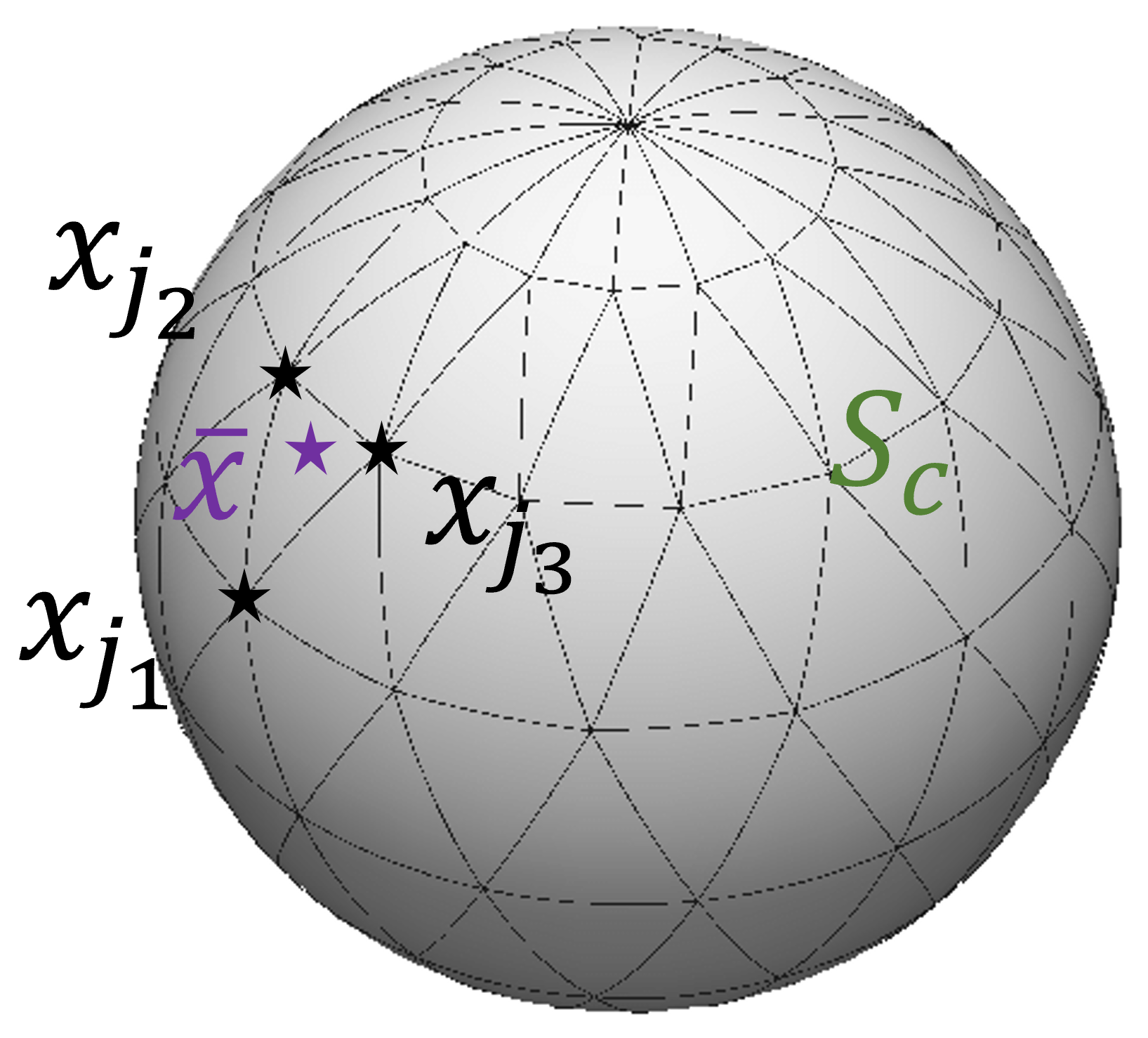
Figure 3: 3-D case: Triangulating sampling of the boundary $\partial S_{c}$.

Now, we show that if the following holds

$$\sup_{u_{v}\in\tilde{\mathcal{U}}_{v}}H(x_{i},u_{v})\leq-l_{H}d_{a}-l_{B}\delta\quad\forall i\in\mathcal{I},$$ (10)

where $l_{B}$ is the Lipschitz constant for $B$ and $\delta,l_{H}$ are as defined in Assumptions 1 and 2, respectively, then, (7) holds. With $c\in[0,c_{M}]$, the set $S_{c}$ is non-empty, and with $d_{a}\in\begin{bmatrix}0,d_{M}\end{bmatrix}$, there exist sufficient points $N_{p}$ to have a polyhedron that can triangulate the boundary $\partial S_{c}$. Under the conditions imposed on $\{x_{i}\}_{\mathcal{I}}$, for every $\bar{x}\in\partial S_{c}$, there exists a triangular face $T_{j}$ with coordinates $x_{j_{1}},x_{j_{2}},x_{j_{3}}\in\{x_{i}\}_{\mathcal{I}}$ satisfying (9) and $0\leq\theta\leq 1$ such that $x_{o}+\theta(\bar{x}-x_{o})\in T_{j}$. Using Lipschitz continuity of $\sup_{u_{v}}H(\cdot,u_{v})$ per Assumption 2, it holds that $\sup_{u_{v}\in\tilde{\mathcal{U}}_{v}}H(\bar{x},u_{v})\leq\sup_{u_{v}\in\tilde{\mathcal{U}}_{v}}H(x,u_{v})+l_{H}|\bar{x}-x|$, for all $x,\bar{x}\in\partial S_{c}$. For $x=x_{i}$, $i\in\mathcal{I}$, using (10) and the fact that $|x-y|\leq d_{S_{c}}(x,y)$ for all $x,y\in\partial S_{c}$, we obtain that

$$\sup_{u_{v}\in\tilde{\mathcal{U}}_{v}}H(\bar{x},u_{v})\leq -l_{H}d_{a}-l_{B}\delta+l_{H}d_{S_{c}}(\bar{x},x_{i}),\;\forall i\in\mathcal{I}.$$

Since the projection of $\bar{x}$ lies in the triangular face $T_{j}$, it holds that $d_{S_{c}}(\bar{x},x_{j_{k}})\leq d_{S_{c}}(x_{j_{l}},x_{j_{k}})$ for $l\neq k$, $l,k\in\{1,2,3\}$. Using this and (9), we obtain

$$\sup_{u_{v}\in\tilde{\mathcal{U}}_{v}}H(\bar{x},u_{v})\leq-l_{H}d_{a}-l_{B}\delta+l_{H}d_{a}=-l_{B}\delta,\;\forall\bar{x}\in\partial S_{c}.$$

Thus, checking the inequality (10) at a finite number of points is a computationally tractable method for assessing whether (7) holds for a given $c$ and $\tilde{\mathcal{U}}_{v}$. Note that for a given $F,B,\tilde{\mathcal{U}}_{v}$ and $\delta$, a smaller value of $d_{a}$ implies that the right-hand side of (10) is less negative, thus, making it easier to satisfy the inequality. At the same time, due to (9), a smaller value of $d_{a}$ requires more sampling points $N_{p}$, and hence, checking the inequality at more points. Thus, there is a trade-off between the ease of satisfaction of (10) and the number of points at which the inequality should be checked.

The above arguments can be generalized to the $n-$dimensional case. Using the sampling approach in [20] for a unit sphere in $n-$dimension, combined with Delaunay Triangulation of the sampling points (see e.g., [21]), an $(n-1)-$dimensional simplex can be obtained. If the compact set $S\subset\mathbb{R}^{n}$ is diffeomorphic to a unit $(n-1)-$sphere, then sampling points on the boundary of $S$ can be obtained using the sampling points for the $(n-1)-$unit sphere. Thus, we study the case when the set $S$ is an $(n-1)-$unit sphere.

Let $\{x_{i}\}_{\mathcal{I}}$, with each $x_{i}\in\partial S_{c}$, denote the set of $N_{p}$ sampling data points on the boundary of the sublevel set $S_{c}$ for a given $c\in[0,c_{M}]$ with $c_{M}$ defined in (6) and $\mathcal{I}\coloneqq\{1,2,\dots,N_{p}\}$. The sampling poins $\{x_{i}\}_{\mathcal{I}}$ constitute a simplex $\mathcal{S}_{\mathcal{I}}$ with $N_{f}>0$ faces, $\mathcal{X}_{1},\mathcal{X}_{2},\dots,\mathcal{X}_{N_{f}}$. For a unit sphere in $\mathbb{R}^{n}$, the minimum number of points in the simplex is $(n+1)$, and the minimum possible value of the maximum of the lengths of its edges is $\sqrt{\frac{2(n+1)}{n}}$. The length, denoted as $d_{a}$, of the corresponding arc-length on the boundary $\partial S_{c}$ is $2r_{c}\sin^{-1}\sqrt{\frac{(n+1)}{2n}}$, where $0\leq r_{c}\leq 1$ is the radius of the sphere $S_{c}$. Thus, with $d_{a}\leq 2r_{c}\sin^{-1}\sqrt{\frac{(n+1)}{2n}}$, there must be at least $(n+1)$ points in the simplex. For the sake of brevity, define $d_{M,n}\coloneqq 2r_{c}\sin^{-1}\sqrt{\frac{(n+1)}{2n}}$. We make the following assumption on the sampling points $\{x_{i}\}_{\mathcal{I}}$.

Assumption 3.

Given $c\in[0,c_{M}]$, the sampling points $\{x_{i}\}_{\mathcal{I}}$ and $d_{a}\in\begin{bmatrix}0,d_{M}\end{bmatrix}$, for each $x\in\partial S_{c}$, there exists a face $\mathcal{X}_{j}$ with vertices $\{x_{j_{1}},x_{j_{2}},\dots,x_{j_{n}}\}\in\{x_{i}\}_{\mathcal{I}}$, where $j\in\{1,2,\dots,N_{f}\}$, of the simplex $\mathcal{S}_{\mathcal{I}}$ generated by $\{x_{i}\}_{\mathcal{I}}$, such that $x_{o}+\theta(x-x_{o})\in\mathcal{X}_{j}$ for some $0\leq\theta\leq 1$, and the following holds:

$$\max_{l\neq m\atop l,m=1,2,\dots,n}d_{S_{c}}(x_{j_{l}},x_{j_{m}})\leq d_{a},$$ (11)

where $d_{S_{c}}(x,y)$ denotes the shortest arc-length between the points $x,y\in\partial S_{c}$.

We have the following result when $S$ is $(n-1)-$unit sphere.

Theorem 1.

Suppose that the function $H$ defined in (5) satisfies Assumption 2. Given $c\in[0,c_{M}]$, $d_{a}\in\begin{bmatrix}0,d_{M,n}\end{bmatrix}$, and the sampling points $\{x_{i}\}_{\mathcal{I}}$, if Assumption 3 and (10) hold, then, (7) holds.

Proof.

With $c\in[0,c_{M}]$, the set $S_{c}$ is non-empty, and with $d_{a}\in\begin{bmatrix}0,d_{M}\end{bmatrix}$, there exist sufficient points $N_{p}$ to have a simplex. Now, consider any point $\bar{x}\in\partial S_{c}$. Under Assumption 3, for every $\bar{x}\in\partial S_{c}$, there exists a face $\mathcal{X}_{j}$ of the simplex $\mathcal{S}_{\mathcal{I}}$, such that the line joining the center of the sphere $S_{c}$ and the point $\bar{x}$ lies on this face. Using Lipschitz continuity of $\sup_{u_{v}}H(\cdot,u_{v})$ under Assumption 2 and (10), it holds that

$$\sup_{u_{v}\in\tilde{\mathcal{U}}_{v}}H(\bar{x},u_{v})\leq \sup_{u_{v}\in\mathcal{U}_{v}}H(x,u_{v})+l_{H}|\bar{x}-x|$$

$$\leq -l_{H}d_{a}-l_{B}\delta+l_{H}|\bar{x}-x|,$$

for all $x,\bar{x}\in\partial S_{c}$. Using the inequality for $x=x_{j_{i}}$, $i\in\{1,\dots,n\}$ and the fact that $|\bar{x}-x_{j_{i}}|\leq d_{S_{c}}(\bar{x},x_{j_{i}})\leq d_{S_{c}}(x_{j_{k}},x_{j_{i}})$ for any $k\neq i$, $k\in\{1,\dots,n\}$ and (11), we obtain that

$$\sup_{u_{v}\in\tilde{\mathcal{U}}_{v}}H(\bar{x},u_{v})\leq -l_{H}d_{a}-l_{B}\delta+l_{H}d_{a}=-l_{B}\delta$$

for all $\bar{x}\in\partial S_{c}$, which completes the proof. ∎

Note that there are three set of parameters that can facilitate satisfaction of (10) in the following manner:

• Set $\tilde{\mathcal{U}}_{v}$: smaller $\tilde{\mathcal{U}}_{v}$ makes it easier to satisfy (10);

• Parameter $c$: larger value of $c$ results in smaller values of $d_{M}$, thus, reducing the right-hand side of (10), and making it easier to satisfy it; and

• Number of sampling points $N_{p}$: larger $N_{p}$ results in smaller value of $d_{M,n}$.

Based on these observations, an iterative algorithm can be formulated to check whether there exists a feasible $c$ and a non-empty set $\tilde{\mathcal{U}}_{v}$, such that (10) holds.

IV-B Iterative algorithm

We formulate our algorithm with the following steps:

• For a given value of $0\leq c\leq c_{M}$, $\tilde{\mathcal{U}}_{v}$ and number of sampling points $N_{p}$, sample $\{x_{i}\}_{\mathcal{I}}$ from the set $\partial S_{c}$ and check if (10) holds for all the sampling points;

• Shrink $\tilde{\mathcal{U}}_{v}$, increase $c$ and repeat steps 1)-2) until the condition (10) is satisfied for all the sampling points, or there does not exist a $c$ and a non-empty set $\tilde{\mathcal{U}}_{v}$;

• Increase $N_{p}$ and repeat steps 1)-3) until (10) holds or the maximum value ($N_{max}$) of $N_{p}$ is reached.

Using these steps, we propose Algorithm 1 which returns a feasible $c$ and a set $\tilde{\mathcal{U}}_{v}$ such that safety is guaranteed for all $x\in S_{c}$ and $u_{v}\in\tilde{\mathcal{U}}_{v}$. In other words, this algorithm can compute the set of initial conditions $S_{c}$, and the set of tolerable attacked inputs via $\tilde{\mathcal{U}}_{v}$ such that the system can satisfy the safety property under attacks. The order in which the parameters $c,\tilde{\mathcal{U}}_{v}$, and $N_{p}$ are tuned can be changed, which can potentially change the output of the algorithm.

Data: $f,g_{v},g_{s},\mathcal{U}_{v},\mathcal{U}_{s},B,d_{a},\varepsilon_{1},\varepsilon_{2},\delta,N_{max},N_{c0}$

1 Initialize: $\tilde{\mathcal{U}}_{v}=\mathcal{U}_{v},c=0,N_{p}=N_{c0}$;

2 while $N_{p}<N_{max}$ do

3       while $c\leq c_{M}$ do

4             Sample $\{x_{i}\}_{\mathcal{I}}$ from $\{B(x)\leq-c\}$;

5             while $\tilde{\mathcal{U}}_{v}\neq\emptyset$ do

6                   if $\{i\in\mathcal{I}\;|\;H(x_{i},u_{v})\!>\!-l_{H}d_{a}\!+\!l_{B}\delta\}\neq\emptyset$ then 

7                  $\hskip 10.0pt\tilde{\mathcal{U}}_{v}=\tilde{\mathcal{U}}_{v}\ominus\varepsilon_{1}$  ;

8                  

9            if $\tilde{\mathcal{U}}_{v}=\emptyset$ then 

10            $\hskip 10.0ptc=c+\varepsilon_{2}$;

11             $\hskip 10.0pt\tilde{\mathcal{U}}_{v}=\mathcal{U}_{v}$;

12            

13      $N_{p}=2\;N_{p}$;

14       $c=0$;

15Return: $\bar{\mathcal{U}}_{v},c$;

Algorithm 1 Iterative method for computing $\tilde{\mathcal{U}}_{v},c$

Remark 1.

If it is unknown which components of the input are vulnerable, then all possible combinations of $u_{v}$ and $u_{s}$ can be considered, and Algorithm 1 can be used to compute $c$ for each such combination. Then, the maximum of all such values can be used to define the set $S_{c}$, guaranteeing the system’s security against attack on any control inputs.

Remark 2.

The computational complexity of Algorithm 1 is only a function of the number of sampling points $N_{p}$ (which, in principle, is a user-defined parameter) and is independent of the non-linearity of the function $F$, and linear in the dimension $n$. Thus, unlike reachability based tools in [22, 11] where the computational complexity grows exponentially with the system dimension $n$, or SOS based tools [10] that are only applicable to a specific class of systems with linear or polynomial dynamics, Algorithm 1 can be used for general nonlinear system with high dimension.

So far, we presented sufficient conditions to establish the safety of the system (1) under attacks (Proposition 1), a sampling-based method to verify these conditions using a finite number of sampling points (Theorem 1), and iterative methods to compute the set of initial conditions and the input constraint set to satisfy these conditions (Algorithm 1). Thus, in brief, using the results in this section, we can compute the viability domain $S_{c}$ and control input constraint set $\tilde{\mathcal{U}}_{v}\subset\mathcal{U}_{v}$, such that for all $x\in S_{c}$ and $u_{v}\in\tilde{\mathcal{U}}_{v}$, there exists a control input $u_{s}\in\mathcal{U}_{s}$ that can keep the system trajectories in the set $S_{c}$ at all times. In the next section, we present a method of computing such a control input using a QP formulation.

V QP based feedback design

In this section, we use the sufficient conditions from the previous section to design a feedback law for the system (1) that guarantees security with respect to the safety property under Assumption 1. We assume that the control input constraint set is given as $\tilde{\mathcal{U}}\coloneqq\tilde{\mathcal{U}}_{v}\times\mathcal{U}_{s}=\{v\in\mathbb{R}^{m}\;|\;u_{j,min}\leq v_{j}\leq u_{j,max}\}$, i.e., as a box-constraint set where $u_{j,min}<u_{j,max}$ are the lower and upper bounds on the individual control inputs $v_{j}$ for $j=1,2,\ldots,m$, respectively. We can write $\mathcal{U}$ in a compact form as $\tilde{\mathcal{U}}=\{v\;|\;A_{u}v\leq b_{u}\}$ where $A_{u}\in\mathbb{R}^{2m\times m},b_{u}\in\mathbb{R}^{2m}$. Furthermore, we assume that the system model (1) is control affine, and is of the form:

$$\dot{x} =f(x)+g_{v}(s)u_{v}+g_{s}(x)u_{s}+d(t,x),$$ (12)

where $f:\mathbb{R}^{n}\rightarrow\mathbb{R}^{n}$, $g_{v}:\mathbb{R}^{n}\rightarrow\mathbb{R}^{n\times m_{v}}$ and $g_{s}:\mathbb{R}^{n}\rightarrow\mathbb{R}^{n\times(m-m_{v})}$ are continuous functions. In this case, the function $H:\mathbb{R}^{n}\times\mathbb{R}^{m_{v}}\to\mathbb{R}$ reads

$$H(x,u_{v})=\inf_{u_{s}\in\mathcal{U}_{s}}L_{f}B(x)+L_{g_{s}}B(x)u_{s}+L_{g_{v}}B(x)u_{v}.$$ (13)

In addition to the safety requirement in Problem 1, we impose the requirement of convergence of the system trajectories of (12) to the origin. To this end, given a twice continuously differentiable, positive definite function $V:\mathbb{R}^{n}\rightarrow\mathbb{R}_{+}$ as a candidate Lyapunov function, we use the condition

$$L_{f}V(x)+L_{g_{s}}V(x)u_{s}+L_{g_{v}}V(x)u_{v}\leq-\zeta V(x)-l_{V}\delta,$$ (14)

where $\zeta>0$, to guarantee convergence of the system trajectories to the origin under $d$ satisfying Assumption 1. We assume that the set $S$ is an $(n-1)$-unit sphere, so that we can use the results from the previous section to compute a viability domain for it, and that $0\in\textnormal{int}(S)$, so that the convergence requirement is feasible. The linear constraints on the control input, and the system model being control affine, helps us formulate a convex optimization problem that can be efficiently solved for real-time control synthesis [9]. We propose the following Quadratic Program (QP) to solve Problem 1. Define $z=(v_{s},v_{v},\eta,\zeta)\in\mathbb{R}^{m+2}$ and for a given $x\in\mathbb{R}^{n}$, consider the following QP:

$$\hskip 10.0pt\min_{z}\quad\frac{1}{2}|z|^{2}+q\zeta$$ (15a)

$$\textrm{s.t.}\;\quad\;\;A_{u}v_{na}\leq \;b_{u},$$ (15b)

$$L_{f}B(x)+L_{g_{s}}B(x)v_{s}\leq -\eta~{}(B(x)+c)$$

$$-\sup_{u_{v}\in\tilde{\mathcal{U}}_{v}}L_{g_{v}}B(x)u_{v}-l_{B}\delta,$$ (15c)

$$L_{f}V(x)+L_{g_{s}}V(x)v_{s}+ L_{g_{v}}V(x)v_{v}\leq-\zeta~{}V(x)-l_{V}\delta,$$ (15d)

where $q>0$ is a constant, $l_{B},l_{v}$ are the Lipschitz constants of the functions $B$ and $V$, respectively, and $c$ and $\tilde{\mathcal{U}}_{v}$ are the output of Algorithm 1. Here, $\eta$ and $\zeta$ are slack variables used for guaranteeing feasibility of the QP (see [23, Lemma 6]). The first constraint (15b) is the input constraints, the second constraint is the CBF condition from Lemma 2 for forward invariance of the set $S_{c}$ and the third constraint (15d) is CLF constraint for convergence of the system trajectories to the origin. Note that the secure input $v_{s}$ is used in both (15c) and (15d), while the vulnerable input $v_{v}$ is only used in (15d).

Let the optimal solution of (15) at a given point $x\in\mathbb{R}^{n}$ be denoted as $z^{*}(x)=(v_{s}^{*}(x),v_{v}^{*}(x),\eta^{*}(x),\zeta^{*}(x))$. In order to guarantee continuity of the solution $z^{*}$ with respect to $x$, we need to impose the strict complementary slackness condition on (15) (see [23]). In brief, if the $i-$the constraint of (15), with $i\in\{1,2,3\}$, is written as $G_{i}(x,z)\leq 0$, and the corresponding Lagrange multiplier is $\lambda_{i}\in\mathbb{R}_{+}$, then strict complementary slackness requires that $\lambda_{i}^{*}G(x,z^{*})<0$, where $z^{*},\lambda_{i}^{*}$ denote the optimal solution and the corresponding optimal Lagrange multiplier, respectively. We are now ready to state the following result.

Theorem 2.

Given the functions $F,d,B,V$ and the attack model (2), suppose Assumptions 1-3 hold. Let $c$ and $\tilde{\mathcal{U}}_{v}$ be the output of the Algorithm 1. Assume that the strict complementary slackness holds for the QP (15) for all $x\in S_{c}$. Then, the QP (15) is feasible for all $x\in S_{c}$, and the control law defined as $k_{s}(x)=v_{s}^{*}(x)$ is continuous on $\textnormal{int}(S_{c})$, and solves Problem 1 for all $x(0)\in X_{0}\coloneqq\textnormal{int}(S_{c})$.

Proof.

Per Theorem 1, the set $S_{c}$ is a viability domain for the system (12) under Assumption 2. Thus, feasibility of the QP (15) follows from [23, Lemma 6]. Note also that with $V$ being twice continuously differentiable and under Assumption 2, the Lie derivatives of the functions $V$ and $B$ along $f,g_{s}$, and $g_{v}$ are continuous. Thus, per [23, Theorem 1], the solution $z^{*}$ of the QP (15) is continuous on $\textnormal{int}(S_{c})$. Finally, since the set $S_{c}$ is compact, it follows from [23, Lemma 7] that the closed-loop trajectories are uniquely defined for all $t\geq 0$. Uniqueness of the closed-loop trajectories, Assumption 1 and feasibility of the QP (15) for all $x\in S_{c}$ implies that all the conditions of Lemma 2 are satisfied and it follows that the set $S_{c}$ is forward invariant for the system (12). ∎

Remark 3.

In this work, only the control input $u_{s}$ is used to achieve safety since it is unknown when the vulnerable input $u_{v}$ comes under an attack. This conservative assumption can be relaxed by utilizing an attack-detection mechanism, which can trigger a switching mechanism from a nominal control design, assuming no attacks, to the proposed method under an attack. We leave this detection-based switching mechanism as part of our future work.

VI Numerical Experiments

To showcase the effectiveness of the proposed method, we present an academic example with the system given as

$$\dot{x}=f(x)+Ax+Bu+d(t,x),$$ (16)

where $A\in\mathbb{R}^{3\times 3}$ and $B\in\mathbb{R}^{3\times 2}$. The input constraint sets are $\mathcal{U}_{1}=\{u_{1}\in\mathbb{R}\;|\;|u_{1}|\leq u_{M1}\}$ and $\mathcal{U}_{2}=\{u_{2}\in\mathbb{R}\;|\;|u_{2}|\leq u_{M2}\}$ for some $u_{M1},u_{M2}>0$. The safe set is $S=\{x\in\mathbb{R}^{3}\;|\;|x|^{2}-1\leq 0\}$ corresponding to the function $h(x)=|x|^{2}-1$, i.e., the safe set is the unit sphere. We use randomly generated matrices $A$ and $B$ such that the pairs $(A,B_{1})$ and $(A,B_{2})$ are controllable, where $B_{1}$ and $B_{2}$ are the first and the second columns of the matrix $B$, respectively. The matrices $(A,B)$ and the function $f$ are

$$A\!=\!\begin{bmatrix}0.61&0.37&2.69\\ -0.06&-1.02&-0.88\\ 1.33&-2.71&0.91\end{bmatrix}\!,B\!=\!\begin{bmatrix}-0.24&0.04\\ 0.32&-0.01\\ -1.12&-0.07\end{bmatrix}\!,f(x)\!=\!0.01\!\begin{bmatrix}x_{1}^{3}+x_{2}^{2}x_{3}\\ x_{2}^{3}+x_{3}^{2}x_{1}\\ x_{3}^{3}+x_{1}^{2}x_{2}\end{bmatrix}.$$

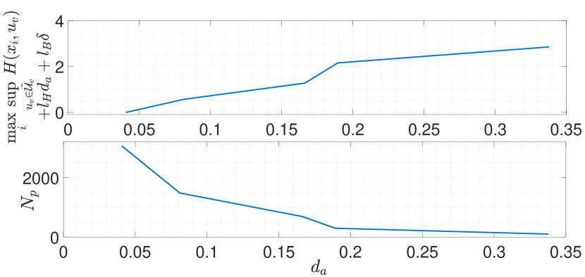
Figure 4: The value of $\max_{i}\sup_{u_{v}\in\tilde{\mathcal{U}}_{v}}H(\bar{x},u_{v})+l_{H}d_{a}+l_{B}\delta+l_{H}d_{a}$ and the number of sampling points for different values of $d_{a}$.

We use MATLAB code from [24] to generate a uniform sampling on the boundary of the unit sphere. Figure 4 shows the maximum value of $\sup_{u_{v}\in\tilde{\mathcal{U}}_{v}}H(\bar{x},u_{v})+l_{H}d_{a}+l_{B}\delta$ over the sampling points for different values of $d_{a}$. It is observed that condition (10) is satisfied when $d_{a}=0.0406$, and the corresponding number of sampling points is $N_{p}=3062$. Without loss of generality, we assume that $u_{2}$ is vulnerable.

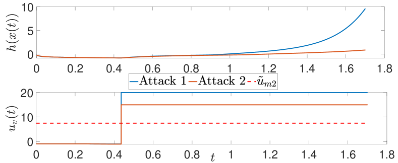
Figure 5: The vulnerable input $u_{v}$ and the function $h$ under attacks 1 and 2.

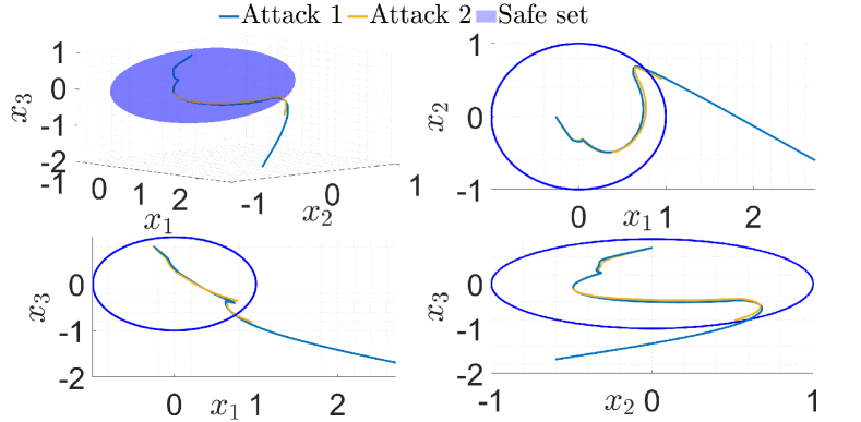
Figure 6: The closed-loop paths traced by the system under attacks 1 and 2.

We use Algorithm 1 to compute the set $\tilde{\mathcal{U}}_{i}$ and a value of $c$ such that (10) holds for all the sampling points. With $u_{M1}=20$ and $u_{M2}=20$ (defining the sets $\mathcal{U}_{s},\mathcal{U}_{v}$), Algorithm 1 gives $c=0$ for the viability domain $\{x\;|\;h(x)\leq c\}$ and $\tilde{u}_{M2}=7.5$ (defining the set $\tilde{\mathcal{U}}_{v}$) as the feasible bound on the attack signal $u_{2}$. The attack happens at a randomly chosen $\tau=0.436$ and $\delta=0.1$ in Assumption 1.

First, we illustrate that the system violates safety when the attack signal $u_{2}$ does not satisfy the bounds computed by Algorithm 1. Figure 5 shows the vulnerable input $u_{v}$ for the initial two attack scenarios (Attack 1 and 2) where $\bar{u}_{M2}=20$ and $\bar{u}_{M2}=15$, i.e., the set $\tilde{\mathcal{U}}_{v}$ is larger than the one computed using the proposed algorithm. Figure 5 also plots the evolution of the barrier function $h$ with time for the two cases. It can be observed that the function $h$ corresponding to this attack takes positive values, and thus, the safety property for the system is violated. Figure 6 plots the corresponding closed-loops paths for the two scenarios, and it can be seen that the system leaves the safe set, thus violating safety.

In the rest of the attack scenarios (Attack 3-6), the bound $|u_{v}|\leq 7.5$ is imposed as computed by the proposed algorithm. Figure 7 plots the different types of attack signals used in these scenarios, namely, saturated signals with $u_{v}=7.5$ and $u_{v}=-7.5$, square wave and sinusoidal signal, both with amplitude $7.5$. The corresponding evolution of the barrier function $h$ illustrates that the system maintains safety in all four scenarios. Figure 8 plots the closed-loops paths for these attack scenarios, and it can be seen that the system trajectories evolve in the safe set at all times, thus maintaining safety. Through this case study, we illustrate that if the system parameters are not chosen according to our proposed method, then there might exist attacks that can lead to violation of safety. On the other hand, when the system parameters are designed according to the proposed algorithm, no attack can violate safety, confirming that the system is secure by design.

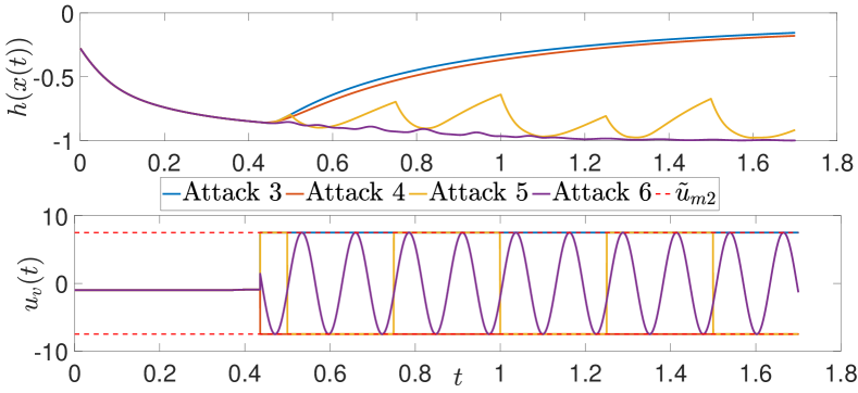
Figure 7: The vulnerable input $u_{v}$ and the function $h$ under attacks 3-6.

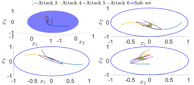
Figure 8: The closed-loop paths traced by the system under attacks 3-6.

VII Conclusion and Future Work

In this paper, we study the problem of computing a viability domain and input constraint set so that the safety of a system can be guaranteed under attacks on the system inputs. In contrast to prior work on the computation of viability domain whose applicability is limited to linear or polynomial dynamics or whose computational complexity grows exponentially with system dimension, our method is computationally efficient and applies to a general class of nonlinear systems. We showed that when the system parameters are chosen using our sampling-based iterative algorithm, the resulting system is resilient to arbitrary attacks, and thus, is secure by design.

Our approach can be used to design bounds (that can either be implemented physically or in a tamper-proof reference monitor) that will prevent attackers from driving control systems to unsafe states. It is efficient (sampling-based viability computation) and general (applicable to non-linear systems). By limiting the range of actuation and the initial set, we are limiting the responsiveness of control action, and in general, systems with our defense might converge slower to the desired set point or trajectory. One way to mitigate this is to use attack-detection mechanisms and switching strategy so that more efficient controllers can be used when the system is not under an attack.

References

- [1] R. M. Lee, M. J. Assante, and T. Conway, “German steel mill cyber attack,” Industrial Control Systems, vol. 30, p. 62, 2014.
- [2] N. E. Oueslati, H. Mrabet, A. Jemai, and A. Alhomoud, “Comparative study of the common cyber-physical attacks in industry 4.0,” in 2019 International Conference on Internet of Things, Embedded Systems and Communications. IEEE, 2019, pp. 1–7.
- [3] A. Cardenas, “Cyber-physical systems security knowledge area issue.” The Cyber Security Body Of Knowledge. [Online]. Available: https://www.cybok.org/media/downloads/Cyber-Physical_Systems_Security_issue_1.0.pdf
- [4] H. Choi, W.-C. Lee, Y. Aafer, F. Fei, Z. Tu, X. Zhang, D. Xu, and X. Deng, “Detecting attacks against robotic vehicles: A control invariant approach,” in Proceedings of the 2018 ACM SIGSAC Conference on Computer and Communications Security, 2018, pp. 801–816.
- [5] V. Renganathan, N. Hashemi, J. Ruths, and T. H. Summers, “Distributionally robust tuning of anomaly detectors in cyber-physical systems with stealthy attacks,” in 2020 American Control Conference (ACC). IEEE, 2020, pp. 1247–1252.
- [6] D. I. Urbina, J. A. Giraldo, A. A. Cardenas, N. O. Tippenhauer, J. Valente, M. Faisal, J. Ruths, R. Candell, and H. Sandberg, “Limiting the impact of stealthy attacks on industrial control systems,” in Proceedings of the 2016 ACM SIGSAC conference on computer and communications security, 2016, pp. 1092–1105.
- [7] A. A. Cárdenas, J. S. Baras, and K. Seamon, “A framework for the evaluation of intrusion detection systems,” in 2006 IEEE Symposium on Security and Privacy (S&P’06). IEEE, 2006, pp. 15–pp.
- [8] M. N. Al-Mhiqani, R. Ahmad, W. Yassin, A. Hassan, Z. Z. Abidin, N. S. Ali, and K. H. Abdulkareem, “Cyber-security incidents: a review cases in cyber-physical systems,” Int. J. Adv. Comput. Sci. Appl, no. 1, pp. 499–508, 2018.
- [9] A. D. Ames, X. Xu, J. W. Grizzle, and P. Tabuada, “Control barrier function based quadratic programs for safety critical systems,” IEEE Transactions on Automatic Control, vol. 62, no. 8, pp. 3861–3876, 2017.
- [10] L. Wang, D. Han, and M. Egerstedt, “Permissive barrier certificates for safe stabilization using sum-of-squares,” in 2018 Annual American Control Conference (ACC). IEEE, 2018, pp. 585–590.
- [11] J. J. Choi, D. Lee, K. Sreenath, C. J. Tomlin, and S. L. Herbert, “Robust control barrier-value functions for safety-critical control,” arXiv preprint arXiv:2104.02808, 2021.
- [12] J. Giraldo, S. H. Kafash, J. Ruths, and A. A. Cardenas, “Daria: Designing actuators to resist arbitrary attacks against cyber-physical systems,” in 2020 IEEE European Symposium on Security and Privacy (EuroS&P). IEEE, 2020, pp. 339–353.
- [13] U. Erlingsson, The inlined reference monitor approach to security policy enforcement. Cornell University, 2004.
- [14] F. Pasqualetti, F. Dörfler, and F. Bullo, “Attack detection and identification in cyber-physical systems,” IEEE transactions on automatic control, vol. 58, no. 11, pp. 2715–2729, 2013.
- [15] S. H. Kafash, J. Giraldo, C. Murguia, A. A. Cardenas, and J. Ruths, “Constraining attacker capabilities through actuator saturation,” in 2018 Annual American Control Conference. IEEE, 2018, pp. 986–991.
- [16] F. H. Clarke, Y. S. Ledyaev, R. J. Stern, and P. R. Wolenski, Nonsmooth analysis and control theory. Springer Science & Business Media, 2008, vol. 178.
- [17] F. Blanchini, “Set invariance in control,” Automatica, vol. 35, no. 11, pp. 1747–1767, 1999.
- [18] K. Garg and D. Panagou, “Robust control barrier and control lyapunov functions with fixed-time convergence guarantees,” in 2021 American Control Conference (ACC), 2021, pp. 2292–2297.
- [19] S. Oudot and J.-D. Boissonnat, “Provably good surface sampling and approximation.” in Symposium on Geometry Processing, 2003, pp. 9–18.
- [20] P. Leopardi, “Diameter bounds for equal area partitions of the unit sphere,” Electron. Trans. Numer. Anal, vol. 35, pp. 1–16, 2009.
- [21] M. De Berg, M. Van Kreveld, M. Overmars, and O. Schwarzkopf, “Computational geometry,” in Computational geometry. Springer, 1997, pp. 1–17.
- [22] S. Bansal, M. Chen, S. Herbert, and C. J. Tomlin, “Hamilton-jacobi reachability: A brief overview and recent advances,” in IEEE 56th Conference on Decision and Control. IEEE, 2017, pp. 2242–2253.
- [23] K. Garg, E. Arabi, and D. Panagou, “Fixed-time control under spatiotemporal and input constraints: A QP based approach,” arXiv preprint arXiv:1906.10091, 2019.
- [24] A. Semechko, “Suite of functions to perform uniform sampling of a sphere,” gitHub. Retrieved August 24, 2021. [Online]. Available: https://github.com/AntonSemechko/S2-Sampling-Toolbox