Protonium annihilation densities in a unitary coupled channel model

Abstract

We consider a unitary coupled channel model to describe the low energy proton-antiproton scattering and the lower Coulomb-like protonium states. The existence of deeper quasi-bound states of nuclear nature is found to be a consequence of the experimental data. The properties of these states as well as the protonium annihilation densities are described and the difference with respect to the optical models description are manifested.

1 Introduction

Several experiments in low energy antiproton physics are based on trapping low energy antiprotons on Coulomb orbits around a nucleus. These processes take usually place at highly excited Rydberg states and, after being captured, the antiprotons cascade down to the lowest Coulomb orbits until they are annihilated with the nucleons. They were experimentally studied in LEAR Amsler_ANP18_87 ; Gastaldi_NPA478_1988 until its closure in 1996 and they are also scheduled in the foreseen PUMA project PUMA_LI_2017 ; PUMA_CERN_Aproval_2021 , both at CERN.

The strong N̄N force results into shiftenning and broadening the antiproton-Nucleus (p̄A) Coulomb states. Their energy becomes complex $E=E_{R}-i\;{\Gamma\over 2}$ and the differences with respect to the pure Coulomb ones $E_{C}$

$$\Delta E\equiv E-E_{C}\equiv\epsilon_{R}-i\;{\Gamma\over 2}$$ (1)

have been measured in several experiments and for a large variety of nuclei. This quantity is a privileged open door for studying and parameterizing the N̄N interaction. To this aim a sizeable amount of low energy scattering data – elastic, annihilation and charge-exchange (p̄p$\to$n̄n) cross sections – as well as the level shifts ($\epsilon_{R}$) and widths ($\Gamma$) of the lowest p̄p (protonium) levels, essentially S and P states, were collected during the LEAR period. The interested reader can find a summary of the most remarkable achievements in the last reviews A_NPA658_99 ; REV_LEAR_KBMR_PREP368_2002 ; REV_LEAR_KBR_PREP413_2005 ; REV_NNB_Frontiers_2020 and references therein.

Of particular interest is the width of a state $\alpha$, $\Gamma_{\alpha}$, where $\alpha=\{L,S,J\}$ denotes the ensemble of its quantum numbers. In the existing theoretical models it can be expressed as an integrated quantity over some spatial distribution in the form

$$\Gamma_{\alpha}=\int_{0}^{\infty}\gamma_{\alpha}(r)\;dr$$ (2)

where $r$ is the distance between the orbiting antiproton and the center of mass of the nucleus. The integrand $\gamma_{\alpha}(r)$, denoted annihilation density, can be interpreted as the probability for an antiproton, captured on a given state $\alpha$, to be annihilated at distance $r$. The knowledge of the annihilation density is relevant in the PUMA project, whose main interest is to correlate the annihilation process with the peripheral density distribution of neutrons in the target nucleus.

Most of the existing NN̄ interaction models are adjusted to reproduce the measured low energy scattering observables REV_NNB_Frontiers_2020 and provide reasonable agreement with the experimentally known protonium $\Delta E$’s Ausberger99 . However the short range part of the pp̄ wave function, determining $\gamma_{a}(r)$, could be strongly dependent on the physical input of the model, in particular the way it mimics the annihilation dynamics.

The aim of the present work is to compare the predictions for $\gamma_{a}(r)$ in the simplest case of protonium, in fact a coupled $\bar{p}p-\bar{n}n$ system, as they are obtained by the two main families of theoretical approaches to NN interaction: optical models (OM) and unitary coupled channel models (UCCM). The protonium annihilation densities have been computed in the past using some selected OM CIR_ZPA334_1989 but no any realistic result is known in the framework of UCCM.

We will describe in Section 2 the main contents of the theoretical N̄N models. Section 3 will be devoted to describe some results with the unitary model concerning N̄N quasi-nuclear states and S-wave protonium level shifts as well as the corresponding annihilation densities. Section contain some concluding remarks.

2 Theoretical models

For the N̄N interactions that we have considered in this work, the real part of the N̄N potential (denoted $U_{\bar{N}N}$) is given by the G-parity transform of an NN model (denoted $V_{NN}$) regularised below some cut-off radius $r_{c}$. The $V_{NN}$’s on which we are interested are in their turn based in meson exchange theory, that is they result from the coherent sum of contributions coming from one-meson exchange potentials $V_{NN}^{(\mu)}$ where $\mu=\pi,\rho,,\omega,..$

$$V_{NN}=\sum_{\mu}V_{NN}^{(\mu)}$$ (3)

For $r>r_{c}$, $U_{\bar{N}N}$ takes the form

$$U_{\bar{N}N}(r>r_{c})=\sum_{\mu=\pi,\rho,\omega,...}\;G(\mu)\;V_{NN}^{(\mu)}(r)$$ (4)

where G($\mu$) is the G-parity of meson $\mu$. G is related to the charge-conjugation (C) and isospin (T) quantum numbers by $G=C(-)^{T}$.

For $r<r_{c}$, a regularization procedure is needed to avoid the non integrable short range singularities (essentially attractive $1/r^{2}$ and $1/r^{3}$ terms) due to the spin orbit and tensor terms. This procedure depends on the particular model.

Thus, the real part of the different N̄N models differ from each other in the choice of their meson content DR1_PRC21_1980 ; DR2_RS_PLB110_1982 ; KW_NPA454_1985 ; CLLMV_PRL_82 ; PLLV_PRC50_1994 ; ELLV_PRC59_1999 ; PARIS_PRC79_2009 ; NNB_CC_Nijm_1984 as well as in the regularization procedures. It is worth noticing however, that during the last years, successful EFT inspired NN̄ potentials have been built Haidenbauer_JHEP_2014 ; Haidenbauer_JHEP_2017 keeping only the pion as the explicit exchanged meson and replacing the heavier ones by contact terms. They are naturally formulated in momentum space and have a strong non local character which make it difficult to be used in configuration space where the annihilation densities are defined. We will not consider them at this stage of our research.

The main differences among the models rely however on the way they account for the annihilation process, giving rise to two main families: optical models (OM) and unitary coupled (UCCM) channel models that we will briefly describe in what follows.

2.1 Optical models

In this approach, the annihilation is described by adding to $U_{\bar{N}N}(r)$ a complex potential $W(r)$ such that

$$V_{N\bar{N}}(r)=U_{\bar{N}N}(r)+W(r)$$ (5)

The imaginary part of $W$ accounts for the loss of flux in the pp̄ channel due to annihilation. In the simplest cases – Dover-Richard version 1 DR1_PRC21_1980 (DR1), version 2 DR2_RS_PLB110_1982 (DR2) and Kohno-Weise KW_NPA454_1985 (KW) – $W$ is local, energy- and state-independent, and have the common form

$$W(r)=-{W_{0}\over 1+e^{r-R\over a}}$$ (6)

with the parameters given in Table 1.

	DR1	DR2	KW
W0 (GeV)	21+20i	0.5+ 0.5i	1.2i
R (fm)	0	0.8	0.55
a (fm)	0.2	0.2	0.2

Table 1: Parameters (GeV and fm) of the Dover-Richard (DR1 and DR2 versions) and Khono-Weise (KW) N̄N optical models.

Although differing either by their meson contents or by their annihilation potential $W$, these three models give similar results for the protonium S- P- and D- waves CIR_ZPA334_1989 .

The Paris NN̄ potential CLLMV_PRL_82 ; PLLV_PRC50_1994 ; ELLV_PRC59_1999 ; PARIS_PRC79_2009 provides a more elaborate non-local, state- and energy-dependent version of $W$ based on the two-meson annihilation and re-annihilation process despicted in Figure 1 that was explictly computed in Bachir_PhD_Paris_1980 . Taking into account this diagram results into a complex annihilation potential $W$ acting in the NN̄ channel with a characteristic range of

$$r_{W}={1\over 2M_{N}}\approx 0.1\;{\rm fm}$$

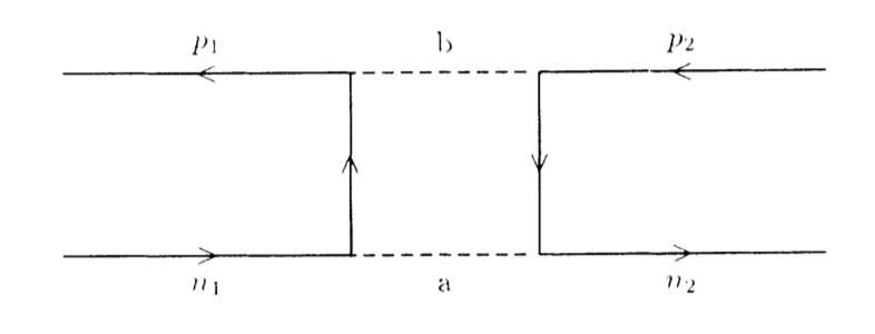
Figure 1: N̄N annihilation into two mesons ($ab$) and re-annihilation into N̄N

The success of OM to describe the phenomenology of low energy pp̄ physics is remarkable REV_NNB_Frontiers_2020 . However the use of complex potentials implies a non hermitian Hamiltonian and a non unitary S-matrix with $\mid U^{\dagger}U\mid<1$. This produces the loss of some standard symmetry properties of the S-matrix and introduce some unphysical properties in the description of bound states and resonances. These drawbacks, first pointed out in KKMS_JETPL26_1977 ; SH_PR35_1978 , have been examined in CDPS_NPA535_91 in the case of KW NN̄ optical potential.

The strong part of NN and NN̄ force is derived in the isospin basis. However this basis is not adapted for computing low-energy pp̄ scattering processes and/or the protonium bound states due to the relevant role of Coulomb interaction and, to a less extend, the p-n mass difference $\Delta_{np}=2(m_{n}-m_{p})$ CIR_ZPA334_1989 . We used instead the so called particle-basis where the $p\bar{p}$ and $n\bar{n}$ states are coupled by the ”charge-exchange potential”. They are described by a two-channel Schrodinger equation

$$(E-H_{0})\Psi=\hat{V}\;\hat{\Psi}$$ (7)

with

$$\quad\hat{\Psi}=\pmatrix{\Psi_{p\bar{p}}\cr\Psi_{n\bar{n}}}\quad\hat{V}=\pmatrix{V_{p\bar{p}}&V_{ce}\cr V_{ce}&V_{n\bar{n}}}$$

and a channel-diagonal kinetic energy term

$$H_{0}=-{\hbar^{2}\over M}\Delta\qquad M={m_{p}+m_{n}\over 2}$$ (8)

Using the isospin conventions Gasiorowicz_1966 ; CIR_ZPA334_1989

$$N={p\choose n}\quad\bar{N}={-\bar{n}\choose+\bar{p}}\equiv\begin{array}[]{lcl}|1/2,+1/2>&=&-|\bar{n}>\cr|1/2,-1/2>&=&+|\bar{p}>\end{array}$$ (9)

the particle basis is expressed in terms of NN̄ isospin states $\mid T,T_{3}>$ as

$$\begin{array}[]{lcl c lcl}|p\bar{p}>&=&+{1\over\sqrt{2}}\left\{|00>+|10>\right\}\\ |n\bar{n}>&=&+{1\over\sqrt{2}}\left\{|00>-|10>\right\}\\ |p\bar{n}>&=&-|1,+1>\\ |\bar{p}n>&=&+|1,-1>\end{array}$$ (10)

and the matrix elements of $\hat{V}$ read

$$V_{p\bar{p}} = {1\over 2}\left({V^{T=0}_{N\bar{N}}+V^{T=1}_{N\bar{N}}}\right)+V_{C}$$ (11)

$$V_{n\bar{n}} = {1\over 2}\left({V^{T=0}_{N\bar{N}}+V^{T=1}_{N\bar{N}}}\right)+\Delta_{np}$$ (12)

$$V_{ce} = {1\over 2}\left({V^{T=0}_{N\bar{N}}-V^{T=1}_{N\bar{N}}}\right)$$ (13)

where $V_{n\bar{n}}$ incorporates the p-n mass difference and $V_{p\bar{p}}$ the Coulomb $p\bar{p}$ interaction

$$V_{C}=-{\alpha(\hbar c)\over r}$$ (14)

For a protonium state $\hat{\Psi}$ with complex energy E, the annihilation density (2) is given by

$$\gamma=\sum_{c=p\bar{p},n\bar{n}}\gamma_{c}$$

where

$$\gamma_{c}=-2\;{\rm Im}[W_{c}(r)]\mid u_{c}(r)\mid^{2}$$ (15)

is the $p\bar{p}$ and $n\bar{n}$ contributions and $u_{c}(r)$ is the corresponding normalised reduced radial wave function, solution of (7). This expression follows from the very definition of a complex eigenstate

$$E=E_{R}-i{\Gamma\over 2}=<\Psi\mid H_{0}+V\mid\Psi>$$ (16)

and the fact that the non hermitian part of the hamiltonian is ${\rm Im}(W)$. This gives

$${\Gamma\over 2}=-\left\{<\Psi\mid{\rm Im}(W)\mid\Psi>\right\}$$ (17)

2.2 Unitary coupled-channels model (UCCM)

This family of models aims to preserve the hermiticity of the full hamiltonian – and consequently the unitarity of the S-matrix – by coupling each NN̄ isospin component to an explicit meson-meson ($m\bar{m}$) channel

$$\mid N\bar{N}\rangle_{T}\qquad\to\qquad\mid N\bar{N}\rangle_{T}=\pmatrix{\Psi^{T}_{N\bar{N}}\cr\Psi^{T}_{m\bar{m}}}$$ (18)

This NN̄$\to$ mm̄ coupling is realised with a short range Yukawa like potential

$$V_{a}^{T}(r)=\lambda_{T}\;(\hbar c)\;{e^{-{r\over r_{a}}}\over r}$$ (19)

corresponding to the diagram of Fig. 2 and which is, abusively, denoted ”annihilation potential”.

Figure 2: N̄N annihilation into two mesons ($m\bar{m}$)

The range ${r_{a}}$ of the annihilation potential (19) thus defined, is given by the nucleon Compton wavelength

$$r_{a}={1\over m_{p}}\approx{0.21\ fm}$$ (20)

This value is in agreement with the views of Refs. MARTIN 61 ; SH_PR35_1978 which define the annihilation range as the nearest singularity of the scattering amplitude (represented in Fig 1) in the $t$-channel. They obtain a lower limit $r_{a}<1/2m_{p}$, which is independent of the number of annihilating mesons along the $t$-channel. It is also in agreement with the characteristic range $r_{W}$ of the Paris annihilation potential Bachir_PhD_Paris_1980 . The question of ”annihilation range” has been abundantly debated in the past; the interested reader can profitably consult Erice_1988 ; Mainz_1988 ; Haidenbauer_ZPA334_1989 ; REV_NNB_Frontiers_2020 and references therein.

This provides for each isospin state, a two-channel Schrodinger equation

$$(E-H_{0})\pmatrix{\Psi^{T}_{N\bar{N}}\cr\Psi^{T}_{m\bar{m}}}=\hat{V}\pmatrix{\Psi^{T}_{N\bar{N}}\cr\Psi^{T}_{m\bar{m}}}$$ (21)

where

$$\hat{V}^{T}=\pmatrix{V_{N\bar{N}}^{T}&V^{T}_{a}\cr V^{T}_{a}&V^{T}_{m\bar{m}}-\Delta}$$ (22)

is a real and hermitian potential matrix and $\Delta=2(M-M_{m})$ accounts for the threshold mass difference between the nucleon-nucleon (NN) and meson-meson (mm̄) channels. We will assume hereafter that $V_{m\bar{m}}=0$, so that mesons interact only via the coupling to NN̄ channel.

The main difference with respect to optical models is that, even for bound states (with Re(E)$>-\Delta$), the second channel is kinematically open and has scattering boundary conditions. This is better illustrated by writing equation (21) in terms of the reduced radial solutions $u_{c}(r)$

$${\hbar^{2}\over 2\mu_{1}}u_{1}^{\prime\prime}+\left[E\;-\;{l_{1}(l_{1}+1)\hbar^{2}\over 2\mu_{1}r^{2}}-V_{11}\right]u_{1} = V_{12}u_{2}$$ (23)

$${\hbar^{2}\over 2\mu_{2}}u_{2}^{\prime\prime}+\left[E\;-\;{l_{2}(l_{2}+1)\hbar^{2}\over 2\mu_{2}r^{2}}+\;\Delta\;\right]u_{2} = V_{21}u_{1}$$ (24)

where $\mu_{c}$ and $l_{c}$ denotes the reduced mass and angular momentum of channel $c=1,2$.

For the S-wave, the asymptotic boundary conditions of channel $u_{c}$ are given by

$$u_{c}(r)=e^{iq_{c}r}$$ (25)

where $q_{c}$ are the channel momenta, related to the energy of the state by

$$q_{1}^{2} = {2\mu_{1}\over\hbar^{2}}E$$ (26)

$$q_{2}^{2} = {2\mu_{1}\over\hbar^{2}}(E+\Delta)$$ (27)

Figure 3: Complex momentum ($K^{i}$)and Energy ($E^{i}$) sheets corresponding to protonium states in the two channels of the unitary coupled-channel model (21)

The different choices for the complex squared root define a multivalued complex momentum (K) and energy (E) manifolds. For the two-channel problem they are represented schematically in Fig. 3, with, the following determinations of the complex squared root :

• For the first channel with $-\Delta<{\rm Re}(E)<0$ and ${\rm Im}(E)\leq 0$, $q_{1}$ is defined with the squared root determination such that ${\rm Re}(q_{1})\leq 0,{\rm Im}(q_{1})>0$, i.e.

  $$q_{1}=-\alpha_{1}+i\beta_{1}\quad e^{iq_{1}r}=e^{-i\alpha_{1}r}e^{-\beta_{1}r}$$ (28)

  It corresponds to a squared integrable solution.

• For the second channel with ${\rm Re}(E+\Delta)>0$, $q_{2}$ is defined with ${\rm Re}(q_{2})>0,{\rm Im}(q_{2})<0$

  It corresponds to a scattering resonant state, that is exponentially increasing

  $$q_{2}=\alpha_{2}-i\beta_{2}\quad e^{iq_{2}r}=e^{i\alpha_{2}r}e^{\beta_{2}r}\quad\alpha_{2},\beta_{2}>0$$ (29)

where $\alpha_{1},\beta_{1}>0$. A more detailed explanation of the non trivial analytical structure of the K- and E-manifolds corresponding to a coupled channel model can be found in BMS_SJNP30_1979 .

The annihilation densities can be obtained by means of a similar expression than for optical models. The formal derivation is however more involved and has been detailed in A.

The final result for the width, is expressed in terms of the annihilation channel wavefunction only

$${\Gamma\over 2}=\left\{{\hbar^{2}\over 2\mu_{2}}\int_{0}^{R}dr\;{\rm Im}[u^{*}_{2}(r)u^{\prime\prime}_{2}(r)]\right\}$$ (30)

and the corresponding annihilation density is given by

$$\gamma_{a}(r)=2\;\left\{{\hbar^{2}\over 2\mu_{2}}\;{\rm Im}[u_{2}^{*}(r)u^{\prime\prime}_{2}(r)]\right\}$$ (31)

which constitutes the UCCM counterpart of (15).

The relevance of an hermitian approach to the N̄N problem was put forward before starting the LEAR era, by I.S. Shapiro and collaborators, from the ITEP and Lebedev groups in Moscow KKMS_JETPL26_1977 ; SH_PR35_1978 ; BMS_SJNP30_1979 . The main reasons were (i) to keep the right analytical properties of the S-matrix which are lost in the optical models due to the non hermitian character and (ii) to have a non vanishing short range $\bar{p}p$ wave function which, due to the strong imaginary part of the optical models, is extremely suppressed. Both facts – together with a short range annihilation potential – have dramatic consequences in the properties (energies and widths) of the S-matrix poles associated with the bound states CDPS_NPA535_91 and in the description of the annihilation process itself. These differences affect both the deeply quasi-bound and resonant states of nuclear origin (the so called ”quasi-nuclear states”, first proposed in DMS_JETPL10_1969 ; DMS_SJNP11_1970 ; DMS_NPB21_1970 ; DMS_PMNP_1971 ), as well as the loosely bound Coulomb-like states of protonium.

As an illustrative example of such a different behaviour we have compared in Figure 4 the complex energy trajectories of a ¹¹S₀ bound state as a function of the annihilation strength obtained in an optical model and in a unitary coupled channel model. This is a pure isospin (T=0) state, generated by the strong N̄N interaction only, hence its ”quasi-nuclear” denotation. The results for the optical model (black dots) are taken from CDPS_NPA535_91 and correspond to KW model. In absence of annihilation ($W_{0}$=0) it is a bound state with energy E=-54.7 MeV and rms radius R=$\sqrt{<r^{2}>}$=1.3 fm. This energy, that become complex for $W_{0}\neq 0$, is plotted as a function of $W_{0}$ defined in (6). We have adjusted the parameters of the UCCM described in the next section, in order to locate a bound state at the same energy and vary the annihilation strength $\lambda$ in the physical domain. The corresponding trajectory $E(\lambda)$ is indicated in red dots.

In OM, the annihilation has always a ”repulsive” effect, that is decreases the real part of the bound state energy and ”pull out” the state towards the continuum; the threshold is crossed at $W_{0}\approx 0.5$ GeV, well before its model value $W_{0}=$1.2 GeV. In a unitary model the situation is totally opposite: in the range of parameters of interest the annihilation has an attractive result, with an increasing energy Re(E). Notice also that the level shift and the width of the state remains much smaller than for OM.

As it was shown in refs KKMS_JETPL26_1977 ; SH_PR35_1978 , the origin of this striking differences – small level shifts and width and effective attraction in the N̄N channel induced by the annihilation – relies ultimately in two model properties: its unitarity and the short range of the annihilation potential. On one hand, while in the optical model the p̄p wave function is systematically suppressed (loss of flux in the p̄p channel that goes nowhere), in the UCCM it is, at the same time and with equal probability, populated by the ”re-annihilation process”, i.e. by the reverse n̄n$\to$p̄p coupling. For small or moderate value of the annihilation strength, the net effect is attractive and the corresponding p̄p wave function can be even enhanced with respect to the free case. On the other hand, if the size of the state is larger than the annihilation range ($r_{a}<<R$) the level shifts and widths of the state are loosely affected by the coupling and remain small.

This example concerns a relatively deep, quasi-bound state of quasi-nuclear nature. We will see in the next section other examples taken from the Coulomb-like protonium states, involving energies several order of magnitude smaller and much larger sizes, where the complex energy trajectories have a different behaviour.

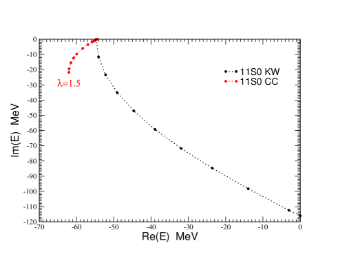
Figure 4: Complex energy trajectory of a ¹¹S₀ state as a function of the annihilation strength in optical a unitary coupled channel models

Exhausting the N̄N annihilation process by a fictitious two-meson channel, furthermore taken interaction free $V_{m\bar{m}}\equiv 0$, is an oversimplification of the physical problem, involving even at zero energy dozens of annihilation channels with many particles in the final state. It is however a consistent way to guarantee the unitarity of the N̄N model and the proper analytic structure of the scattering amplitudes. The unitarity relies on the use of a real transition potential (19) inserted in the symmetric potential matrix (22) of an hermitian equation (21).

This fact and the existence of two different interaction ranges ($r_{N}\sim 1$ fm in the NN̄ chanel, $r_{a}\sim 0.2$ fm in the NN̄$\rightarrow$mm̄ transition potential), constitute the key points of this approach. The UCCM approach has been successfully used in many problems related to baryon-antibaryon states DPS_IJMPA5_1990 ; DCP_SJNP52_1990 ; CPD_NP558_1993 ; CPD_PLB306_1993 ; DCK_NCA107_1994 but it has never been applied to describe with realistic interactions the level shifts of protonium low lying states, or equivalently the $p\bar{p}$ scattering lengths. This will be done in the next section for a particular choice of $V_{N\bar{N}}$.

3 Results from a unitary coupled-channels model

3.1 The model

The N̄N unitary coupled channel model that we have considered is a modified version (hereafter denoted Model I) of that used in DCP_SJNP52_1990 ; CPD_NP558_1993 ; CPD_PLB306_1993 ; DCK_NCA107_1994 for describing the low energy nucleon-antinucleon interaction at $p_{lab}<300$ MeV/c as well as the $p\bar{p}\to\Lambda\bar{\Lambda}$ nearthreshold phenomena.

The meson contents of the NN̄ interaction – two pseudoscalar ($\pi,\eta$), two vector ($\rho,\omega$) and two scalars ($\sigma_{0},\sigma_{1}$) – was taken from the pioneering Brian-Phillips work BP_NPB5_1968 with an updated $\pi N$ coupling constant. The corresponding masses, quantum numbers and couplings are given in Table 2.

$$\begin{array}[]{ c c c c c c c }1&m&J^{\pi}&T&G&g&f/g\\ \hline\cr\pi&138.2&0^{-}&1&-&13.5&-\\ \eta&548&0^{-}&0&+&7.0&-\\ \rho&760&1^{-}&1&+&0.68&4.4\\ \omega&782&1^{-}&0&-&21.5&0\\ \sigma_{0}&770&0^{+}&1&-&6.1&-\\ \sigma_{1}&560&0^{+}&0&+&9.4&-\end{array}$$

Table 2: Meson coupling constants for the $\bar{N}N$ potential

The original model, formulated in the isospin basis, has been readjusted in view of describing the protonium states, with the isospin symmetry broken by the Coulomb forces and the $pn$ mass difference. Indeed, it appeared necessary to work from the very beginning on the pp̄-nn̄ particle basis and properly account for the nn̄ threshold and Coulomb effects. These effects, as well as the tensor coupling potential, were not taken into account in the previous calculations DCP_SJNP52_1990 ; CPD_NP558_1993 ; CPD_PLB306_1993 ; DCK_NCA107_1994 . Its importance will be discussed in the next sections.

As it was the case for optical models the p̄p and n̄n channels are coupled to each other via the charge exchange potential ($V_{ce}$). Each of them is in addition coupled to a meson-meson channel via the so called annihilation potentials ($V^{a}$). The meson-meson interaction is neglected but, as for the nn̄ channel (13), the corresponding potential incorporates the threshold mass difference $\Delta$=$2(M_{p}-M_{m})$. This results into a real hermitian potential matrix which guarantees the unitarity and has the following structure:

$$\hat{V}=\pmatrix{V_{p\bar{p}}&V_{p\bar{p}}^{a}&V_{ce}&V_{ce}^{a}\cr V_{p\bar{p}}^{a}&-\Delta&V_{ce}^{a}&0\cr V_{ce}&V_{ce}^{a}&V_{n\bar{n}}&V_{p\bar{p}}^{a}\cr V_{ce}^{a}&0&V_{n\bar{n}}^{a}&-\Delta}$$ (32)

where the components $V_{p\bar{p}}$, $V_{n\bar{n}}$ and $V_{ce}$ in (32) are expressed in terms of the isospin components as for the OM case (13) and the annihilation potentials given by

$$V^{a}_{p\bar{p}}(r) = {\lambda_{0}+\lambda_{1}\over 2}\;{e^{-{r\over r_{a}}}\over r}$$ (33)

$$V^{a}_{ce}(r) = {\lambda_{0}-\lambda_{1}\over 2}\;{e^{-{r\over r_{a}}}\over r}$$ (34)

The state vector consist in a four channel vector obeying a Schrodinger equation

$$(E-H_{0})|\Psi>=\hat{V}|\Psi>\hskip 28.45274pt|\Psi>=\pmatrix{p\bar{p}\cr m\bar{m}\cr n\bar{n}\cr m\bar{m}}$$ (35)

in which E is the center of mass energy energy with respect to the pp̄ threshold.

Equation (35) can be solved in differential form after a partial wave analysis of each channel wave function. This gives for the reduced radial wave functions $u_{\alpha}(r)$ a system of coupled differential equations

$$u_{\alpha}^{\prime\prime}+\left[k_{\alpha}^{2}-{L_{\alpha}(L_{\alpha}+1)\over r^{2}}\right]u_{\alpha}-\sum_{\beta}v_{\alpha\beta}u_{\beta}=0$$ (36)

where $v_{\alpha\beta}$=${2\mu_{\alpha}\over\hbar^{2}}V_{\alpha\beta}$ and $\alpha(\beta)$ label the channel and partial wave quantum numbers $\{L,S,J\}$, and the channel momenta $k_{\alpha}$, defining the asymptotic boundary conditions, are given by the relation

$$k_{\alpha}^{2}={2\mu_{\alpha}\over\hbar^{2}}\;[E+2(M_{p}-M_{\alpha})]$$

ensuring the same total c.o.m. energy in all of them $\sqrt{s}=2\sqrt{M_{\alpha}+k_{\alpha}^{2}}\approx 2M_{i}-k_{i}^{2}/M_{i}$. Notice that when using the differential form (36) the threshold mass differences ($\Delta$’s) must be removed from the potential matrix (32).

The masses $M_{i}$ of the different channels are respectively $M_{1}$=$m_{p}$=938.28 MeV, $M_{2}$=$m_{n}$=$m_{p}$+1.2933 MeV, $M_{2}$=$M_{4}$=763.0 MeV.

We will use all along this paper the standard spectroscopic notation ^(2S+1)L_J, eventually completed with isospin ^(2T+1)(2S+1)L_J. For the uncoupled states (¹S₀, ¹P₁, ³P₀,…) the number of coupled Schrodinger equations (36) is 4 and the case of tensor coupled states (e.g: ${}^{3}SD_{1}$, ${}^{3}PF_{2}$,…) this number is doubled.

The singularities at $r$=0 due to the spin-orbit and tensor terms of $V_{N\bar{N}}$, are regularised by imposing, below some cutoff radius $r_{c}$, a $C^{1}$ polynomial matching in the form:

$${V(x)}={V_{0}}+Ax^{\nu}+Bx^{\nu+1}$$ (37)

where $x={\left(r\over{r_{c}}\right)}$. The coeficients $A$ and $B$ are determined by the matching conditions. We have fixed the value $V_{0}$=0 to minimise the short range effects of a potential which is anyway unknown at small distances, and we have examined the two extreme cases $\nu$=1 and $\nu$=10. The final result is a smoothed version of the OBE potential suitable for numerical calculations. This regularisation procedure is implemented to each isospin component of a given partial wave $\alpha\equiv\{S,L,J\}$.

To check the stability of the OBE predictions in $U_{N\bar{N}}$, we have also considered an alternative model (denoted Model II) built with the meson contents of the Nijmegen N̄N potential NNB_CC_Nijm_1984 although regularised with the same prescription (37). This model contains a different set of mesons $(\pi,\eta,\eta^{\prime},\rho,\phi,\omega,\epsilon)$ with slightly different coupling constants. In general Model II results into a weaker potentials, specially in the T=0 channel, due to the stronger cancellations among the mesons. This is compensated by using a smaller values of $r_{c}$, but the main conclusions were found qualitatively the same in both cases.

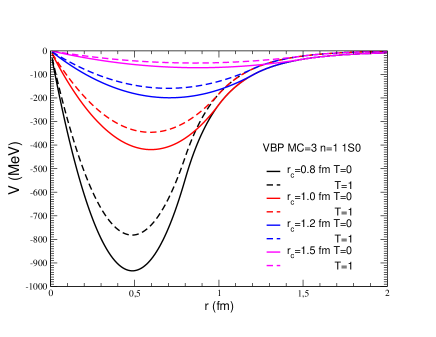
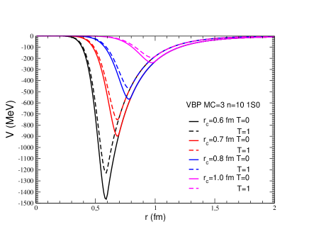
Figure 5: Regularized OBE part of the NN̄ potential in the ${}^{1}S_{0}$ partial wave with parameters $\nu$=1 (upper panel) and $\nu$=10 (lower panel ) in (37) and different values of the cut-off parameter $r_{c}$

We have plotted in Figure 5 the isospin components of the NN̄ potential (Model I) for the ${}^{1}S_{0}$ partial waves corresponding to $\nu$=1 (upper panel) and $\nu$=10 (lower panel) in (37) and for different values of the cut-off parameter $r_{c}$. The interaction is reconstructed ”inwards” through the peripheral meson-nucleon coupling constants, in principle the best well stablished one. In particular, for $\nu=$10 the interaction becomes negligible below $r\approx r_{c}$.

The lower quasi-nuclear spectra of the ¹S₀ state as a function of the cut-off radius $r_{c}$ is displayed in Figure 6. It corresponds to Model I (BP) with $\nu$=1. Colored lines correspond to the uncoupled isospin states (blue for T=0, and red for T=1) while the solid black lines to the ground (n=1) and first excited (n=2) coupled pp̄-nn̄ states. One sees that the effect of isospin coupling, due to Coulomb and $\Delta_{np}$, becomes negligible below few MeV but it can account for 1 MeV difference nearthreshold, that is precisely in the region of Coulomb like protonium states. The infinity of states, generated by Coulomb term (14) and with energies of few KeV, are not represented in the figure.

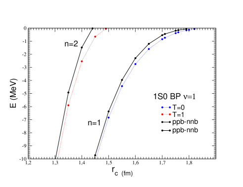
Figure 6: Spectra of the ¹S₀ state with BP potential (Model I) with $\nu$=1 as a function of the cut-off radius $r_{c}$. Dashed coloured lines correspond to pure isospin (T) states and black solid lines to the coupled p̄p-n̄n ground (n=1) and first excited (n=2) states including Coulomb and $\Delta_{np}$ terms.

In summary, the models we have considered contain two parameters for each partial wave $\alpha$=$\{L,S,J\}$: the cut-off radius $r_{c}$ and the dimensionless annihilation strength $\lambda$. This gives two free parameters per uncoupled states (¹S₀,¹P1, ³P₀…). For the tensor coupled states, e.g. ³SD₁, this means 2 parameters for ³S₁, 2 for ³D₁ plus an additional cut-off parameters $r_{T}$ needed to regularise the tensor coupling potential $V_{{}^{3}S_{1}\to^{3}D_{1}}$.

Next section will be devoted to present the scattering results.

3.2 Protonium S-waves scattering lengths

Our aim is to fix the model parameters ($r_{c},\lambda$) for the protonium S-waves in order to reproduce the experimental values of the singlet ($a_{0}$) and triplet ($a_{1}$) $p\bar{p}$ scattering lengths. These values are not directly measured but we have extracted them from the measured Ausberger99 protonium level shifts and widths (1) by means of the Trueman expansion Trueman_NP26_1961 in the way described in CRW_ZPA343_1992 . The results for $\Delta E$ and $a_{s}$ are given in Table 3 together with the predictions of the KW optical model obtained in CIR_ZPA334_1989 .

	Exp A_NPA658_99	KW CIR_ZPA334_1989 ; CRW_ZPA343_1992
$\Delta E({{}^{1}S_{0}})$	0.440(75) - i 0.600(125)	0.50-i 0.63
$\Delta E({{}^{3}SD_{1}})$	0.785(35) - i 0.470(40)	0.78-i 0.49
a0(${}^{1}S_{0}$)	0.49(9) - i 0.73(14)	0.57- i 0.77
a1(${}^{3}SD_{1}$)	0.93(4) - i 0.60(5)	0.92- i0.63

Table 3: Experimental S-wave protonium complex energy shifts $\Delta E$ (in keV) and pp̄ scattering length $a_{s=0,1}$ (in fm) together with the KW optical model predictions taken from CIR_ZPA334_1989 ; CRW_ZPA343_1992 . The experimental $a_{s}$ values are extracted from the measured $\Delta E$ by means of the Trueman relation Trueman_NP26_1961 .

For methodological reasons we have proceeded in two consecutive steps.

As a first step we have studied the dependence of the singled ¹S₀ $\bar{p}p$ scattering length $a_{0}$ as a function of the cut-off radius $r_{c}$ in absence of any annihilation, i.e. $\lambda(^{1}S_{0})=0$. The results for Model I (BP) are displayed in Figure 7 for the two regularisation parameter values $\nu$=1 (upper panel) and $\nu$=10 (lower panel). The blue horizontal lines correspond to the experimental value of Re[$a_{0}$]=0.49(9) fm.

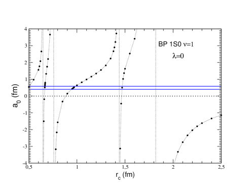
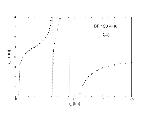
Figure 7: ¹S₀ $\bar{p}p$ scattering as a function of the $r_{c}$ without coupling to annilihation channels with Model I regularization parameter $\nu$=1 (upper panel) and $\nu$=10 (lower panel) in (37)

One can see that for large values of $r_{c}$ the sign of $a_{0}$ is negative, while the experimental value has $\mathrm{Re}(a)=0.49(9)>0$. This negative sign corresponds to an attractive $p\bar{p}$ potential, obtained by averaging the isospin components of $V_{N\bar{N}}$ displayed in Figure 5 plus the attractive Coulomb force. When $r_{c}$ is decreased, $V_{p\bar{p}}$ becomes increasingly attractive until the first $p\bar{p}$ bound state appears. This corresponds to a divergence of $a_{0}$ which happens at $r_{c}\approx 1.8$ fm for $\nu$=1 (see also Figure 6) and $r_{c}\approx 1.4$ for $\nu$=10. In order to obtain a positive scattering length we are obliged to accommodate one (or several) bound states.

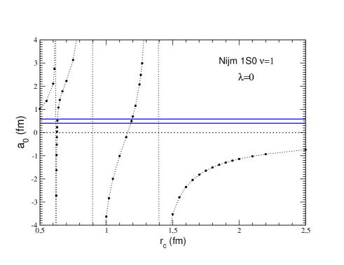
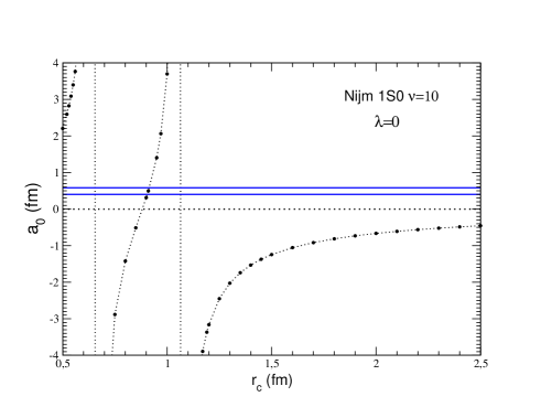
Figure 8: The same than Figure 5 for Model II, based on Nijmegen meson exchange potential of NNB_CC_Nijm_1984 .

The same conclusion is reached in Model II, when using the NN̄ potential built with the Nijmegen meson contents of Ref. NNB_CC_Nijm_1984 . The results are represented in Figure 8, with $\nu$=1 in the upper part and $\nu$=10 in the lower one. Nijmegen potential is much weaker than BP specially for the T=0 components – due to the greater number of mesons involved that favours large cancelations between their contributions – but it displays the same qualitative result with the first singularity at $r_{c}\approx 1.4$ fm for $\nu$=1 and $r_{c}\approx 1.1$ fm for $\nu$=10.

Thus, we would like to emphasize that the existence of quasi-nuclear states (or baryonium) suggested by Dalkarov, Shapiro and Mandeltsveig 50 years ago DMS_JETPL10_1969 ; DMS_SJNP11_1970 ; DMS_NPB21_1970 ; DMS_PMNP_1971 , appears to be a natural, and unavoidable, consequence of the long range part of the NN interaction itself.

One could argue that a repulsive $V_{p\bar{p}}$ potential could also generate a pp̄ Re[$a_{0}>0$] value without requiring any underlying bound state. However this is in contradiction with the bulk of experimental data SH_PR35_1978 as well as with all the existing N̄N meson-exchange inspired models. It would be very interesting to see whether a pionless EFT inspired N̄N model, with low energy constants directly fitted to experimental results, reach the same conclusion in what concerns the N̄N spectra.

In absence of any annihilation process we have at our disposal several solutions to reproduce the experimental Re($a_{0}$): those given by the intersection of the $a_{0}(r_{c})$ curve with the two solid blue horizontal lines representing the experimental value with the error band. For Model I, based on BP potential, the solutions displayed in Fig. 7 are: for $\nu$=1 $r_{c}^{(1)}\approx 1.47$ and $r_{c}^{(2)}\approx 0.96$, while for $\nu$=10 $r_{c}^{(1)}\approx 1.10$ and $r_{c}^{(2)}\approx 0.70$. For Model 2, based on Nijmegen potential, the results are displayed in Fig. 8. For $\nu$=1 they give $r_{c}^{(1)}\approx 1.2$ fm, $r_{c}^{(2)}\approx 0.6$ fm while with $\nu$=10 one sees a unique solution with $r_{c}\approx 0.9$ fm. Notice that other solution could exist for smaller values of $r_{c}$, and so involving increasingly larger potentials, but we are rather interested in the more peripheral ones. To this aim, Model I allows to use systematically larger cut-off values.

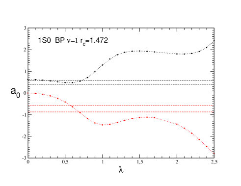
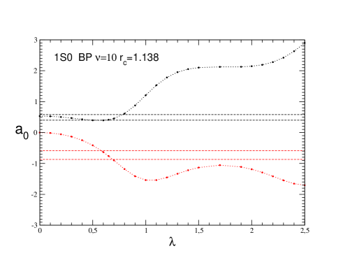
Figure 9: ¹S₀ $\bar{p}p$ scattering length (fm) as a function of the annihilation strength $\lambda$ for Model I: upper panel corresponds to $\nu=$1 (with $r_{c}$=1.472 fm) and lower to $\nu$=10 (with $r_{c}$=1.138 fm). Black solid lines indicate Re($a_{0}$) and red ones Im($a_{0}$). Horizontal dashed lines indicate the corresponding experimental value from Table 3.

The second step consists in keeping fixed the $r_{c}$ values previously determined and switching-on the annihilation potential. The effect of the annihilation potential modifies only slightly the $r_{c}$ values determined at $\lambda$=0. For Model I, we have taken the largest solutions of the $\lambda$=0 case, i.e. $r_{c}$=1.472 fm for $\nu=1$ and $r_{c}$=1.138 fm for $\nu$=10, and we have increased the (dimensionless) annihilation strength $\lambda$ step by step. The results are displayed in Figure 9, upper panel for $\nu$=1 and lower for $\nu$=10. Black solid lines indicate the real part of $a_{0}$ and red ones its imaginary part. Dashed horizontal lines represents a band with the experimental values from Table 3 including errors, in black for the real part and in red for the imaginary part. As one can see the two values of $\nu$ give quite similar results and one obtains a satisfactory description with $\lambda$=0.60 (for $\nu$=1) and with $\lambda$=0.65 for $\nu$=10. Furthermore, this solution seems to be unique for a given $r_{c}$.

The same results corresponding to Nijmegen potential (Model II) are given in Figure 10 . The first ¹S₀ solution for $\nu=1$ is obtained with the parameter values ($r_{c}$=1.20 fm, $\lambda$=1.10).

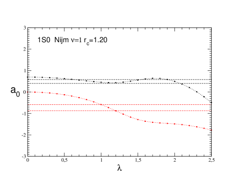
Figure 10: Same as Figure 9 but with Model II based on Njimegen potential and $\nu$=1.

A similar study has been performed for the tensor coupled spin-triplet state ³SD₁ in the two considered models.

For BP potential (Model I), the $a_{1}$ dependence on the cut-off radius is shown in the upper panel of Figure 11. Again, for large $r_{c}$ values the scattering length is negative, contrary to the experimental value, and becomes positive only after the the first bound state appears. That happens at $r^{(1)}_{p}\approx 1.9$ for $\nu$=1. Several other bound state exist at smaller values $r^{(2)}_{p}\approx 1.53$ fm, $r^{(3)}_{p}\approx 1.09$ fm … The qualitative behaviour of $a_{1}(r_{c})$ is quite close to the singlet ¹S₀ one (upper panel of Figure 7). However, due to the strongness of the triplet NN̄ potentials, the $a_{1}(r_{c})$ dependence displays a much richer structure of bound states and a larger number of solutions than for ¹S₀. By selecting the most peripheral solution compatible with the experimental Re[$a_{1}$] ($r^{(1)}_{c}\approx 1.67$ fm for $\nu$=1) and switching on the annihilation, one can reproduce the protonium ³SD₁ data with the parameters values ($r_{c}$=1.67 fm ,$\lambda=1.30$). This is shown in the lower panel of Figure 11.

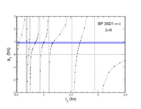
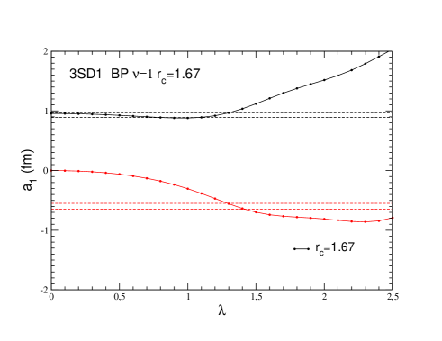
Figure 11: Upper panel : ³SD₁ $\bar{p}p$ scattering length as a function of $r_{c}$ without coupling to annihillation channels with Model I parameters and $\nu$=1. Lower panel $\lambda$-dependence at fixed $r_{c}$=1.67 fm.

By considering Model II, based on Nijmegen potential, the same qualitative agreement is found. We have displayed in Figure 12 (upper panel) the corresponding $a_{1}$ dependence on $r_{c}$ with $\lambda$=0 and in the lower panel its $\lambda$-dependence for $r_{c}=1.52$ fm. This provides a solution reproducing the experimental data with ($r_{c}$=1.52 fm, $\lambda$=1.80).

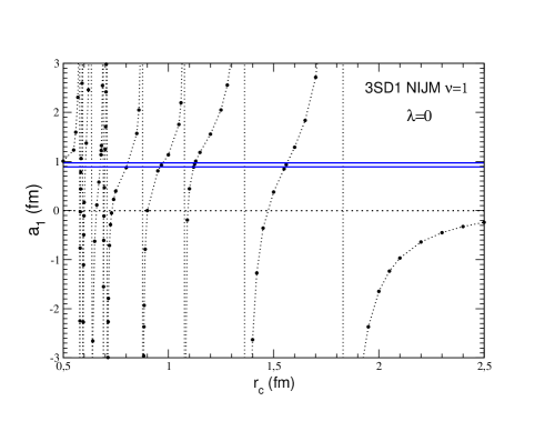
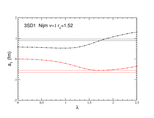
Figure 12: The same than figure 11 for Model II based on Nijmegen potential. Upper panel : ³SD₁ $\bar{p}p$ scattering length as a function of $r_{c}$ without coupling to annihillation channels. Lower panel $\lambda$-dependence at fixed $r_{c}$=1.52 fm.

All together, this allowed us to determine the S-wave model parameters, which are listed in Table 4. Notice that the cut-off radii of Model I are systematically larger than those of Model II and the corresponding annihilation strengths $\lambda$ are smaller.

Model I
State	$\nu$	$r_{c}$(fm)	$\lambda$	$a_{0}$ (fm)
${}^{1}S_{0}$	1	1.47	0.60	0.495 -i 0.747
		0.93	1.91	0.498 -i 0.716
	10	1.14	0.65	0.458 -i 0.770
${}^{3}SD_{1}$	1	1.67	1.30	0.936 -i 0.556
	10	1.31	1.55	0.934 -i 0.608

Model II
State	$\nu$	$r_{c}$(fm)	$\lambda$	$a_{0}$ (fm)
${}^{1}S_{0}$	1	1.20	1.10	0.438 - i 0.724
	10	0.91	1.40	0.446 - i 0.785
${}^{3}SD_{1}$	1	1.52	1.75	0.948 - i 0.549
	10	1.18	2.00	0.800 - i 0.480

Table 4: Computed pp̄ scattering lengths and corresponding parameters with Models I and II

Notice also that although the solutions allow relatively large cut-off values, the role of the OBE contributions in the resulting N̄N potential is essential. Indeed, at $r\approx 1.4$ fm, the strong NN̄ potential displayed in Figure 5 is $\sim$ 30 MeV, while the Coulomb pp̄ potential is $\sim$ 1 MeV. Even at such distances the NN̄ interaction is dominated by one-boson exchanges, mainly pion but still sizeable contributions from heavier mesons.

3.3 Protonium level shifts and annihilation densities

Once the potential parameters have been fixed by reproducing the experimental $p\bar{p}$ scattering lengths, the four-channel homogeneous Schrodinger equation (35) for protonium bound states was solved in coordinate space, using a spline decomposition.

Thus, using the parameters of Mode I ($\nu=1$) displayed in Table 4 we have obtained for ¹S₀ state, a level shift $\epsilon_{R}$=0.427 keV and $\Gamma$= 1.300 keV ($r_{c}$=1.472, $\lambda$=0.65) and a level shift $\epsilon_{R}$=0.426 keV and $\Gamma$=1.278 keV ($r_{c}$=0.93, $\lambda$=1.91). As expected, these protonium $\Delta E$’s are in good agreement with the experimental data from Table 3. In addition we have at our disposal the corresponding realistic S-wave protonium wavefunctions in the framework of a UCCM to obtain the corresponding annihilation densities.

It is worth noticing here that, despite UCCM gives similar prediction than optical models – both are adjusted to this aim ! – there are substantial differences in their underlying dynamics and the short range wave functions.

The first one concerns the dependence of the complex energies $E$ on the annihilation strength. This was already anticipated at the end of section 2.2 for a deeply bound quasi-nuclear state and we will now examine the differences in a Coulomb-like, loosely bound, protonium state. To this aim we have displayed in Fig. 13 the trajectory of $\Delta E$ in the complex energy plane for the ${}^{1}S_{0}$ state as described by the UCCM (black and blue symbols, corresponding to two different solutions $r_{c}=$1.472 fm and $r_{c}$=0.93 fm) and the Khono-Weise OM (red symbols). These trajectories are parametrised by the annihilation strength: $W_{0}$ in OM and $\lambda$ in UCCM. Both of them end up close to the experimental point (denoted by a filled blue square) and are compatible within errors. The maximal annihilation strength is $W_{0}$=1.2 GeV for OM, and $\lambda=0.65$ and $\lambda$=1.91 for UCCM.

Its behaviour is not trivial, when compared to the deeply bound state of Figure 4. For moderate values of $\lambda$ or $W_{0}$, Im(E) is in both cases monotonously increasing. However, while for UCCM Im(E)($\lambda$) remains increasing, in OM the width of the state saturates at $W_{0}\approx 0.7$ GeV and start to decrease for $W_{0}>1$ GeV. The real part of $\Delta E$ (level shifts $\epsilon_{R}$) evolves in opposite directions than for the deeply bound state. For OM the effect of annihilation becomes attractive, i.e. decreasing $\epsilon_{R}$, for all values of $W_{0}$, while in the UCCM the attraction is limited to moderate value of $\lambda$ and becomes repulsive only close to the maximal values of $\lambda$ ($\lambda\approx$ 0.5 for $r_{c}$=1.427 fm and $\lambda\approx$ 1.8 for $r_{c}$=0.93 fm). The difference with respect to the deeply bound state are due to the structure of the wave function. In the former case the size of the state is $\sim$ 1 fm, a spatial region where the annihilation process takes place, while for the protonium states its spatial dimension is given by the Bohr radius $B\approx$ 57 fm.

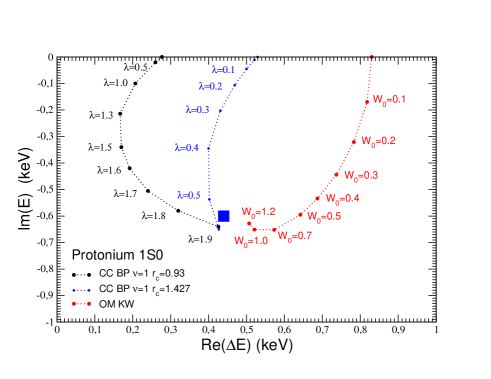
Figure 13: Evolution of the ¹S₀ complex level shifts $\Delta E$ as a function of the annihilation strength for UCCM (dashed black and blue lines) and OM (red dashed lines).

The second one concerns the annihilation densities $\gamma$. We have plotted in Figure 14 the function $\gamma(r)$ of the same protonium ¹S₀ state described with the UCC-Model I (in red) and the Kohno-Weise optical model (in blue). Both models reproduce equally well the experimental values of Table 3, in particular the total width of the state $\Gamma$, i.e. the surface below $\gamma$. However the annihilation process takes place in quite different ways: in the UCCM it is peaked around $r\approx 0.15$ fm, given by the annihilation range $r_{a}$ of Figure 2, and spread over $\Delta r\approx 0.3$ fm, in OM is peaked around $r\approx 0.9$ fm and has a larger dispersion $\Delta r\approx 1$ fm. In the latter case it is difficult to relate the spatial distribution of $\gamma$ with the parameters of the annihilation potential $W(r)$ given in Table 1, since different choices produce quite similar results for $\gamma$ CIR_ZPA334_1989 .

These differences are due to the way in which the annihilation is modelled, as it was described in previous sections 2.1 and 2.2. Although describing the same total width $\Gamma$, they introduce a strong model dependence in the way we understand this process, in particular its spatial distribution. In one case (UCCM), annihilation is a short range ($r_{a}$) process well localised in the p̄p inter-particle distances while in the OM it is spread over a sizeable spatial region. The origin of these differences is also due to the striking differences in the short range part of the p̄p wave function.

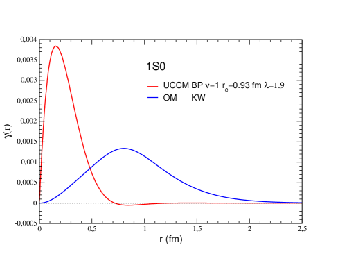
Figure 14: Protonium annihilation density for the ¹S₀ state described with the UCCM (in red) and with OM (in blue). Both models reproduce the same experimental complex level shift $\Delta E$ value of Table 3.

It is indeed interesting to compare the $p\bar{p}$ wave functions provided by the UCCM with the results of the optical model and with the pure Coulomb wave function. This is done in Fig. 15 where we have displayed the modulus squared of the reduced radial wave function $u(r)$ for the protonium ¹S₀ state (first channel). As one can see the results of the UCCM (black solid line) differ considerably from those of the KW optical model (dashed red line), in particular for small values of $r$. In fact for $r\leq 0.5$ fm, where the annihilation process take place, the OM wave function is significantly damped with respect to both the UCCM and the Coulomb (dashed blue line). At $r=0.15$ fm e.g. the CC wave function is two orders of magnitude smaller than the OM one and it is even larger than the Coulomb one despite the annihilation process. As it was already mentioned, this striking differences are a direct consequence of the unitarity.

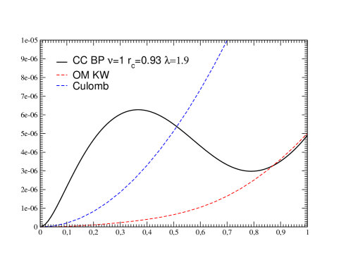
Figure 15: Modulus squared of the 1S0 $p\bar{p}$ radial wave function in UCCM (solid black line) compared with the KW optical model (in dashed red) and the pure Coulomb results (blue dashed line.

4 Conclusion

We have considered a unitary coupled channel model to describe the experimentally measured S-wave proton-antiproton scattering length and the corresponding hydrogen-like singlet and triplet protonium states.

The NN̄ interaction is obtained from a G-parity transform of two different meson-exchange inspired NN models, regularized at short distance. We have shown that, in this theoretical framework, the existence of deep quasi-bound states of nuclear nature is an unavoidable consequence of the protonium experimental data.

The properties of these two types of states – quasi-nuclear and hydrogenic – have been described and the differences with respect to the optical models description have been analyzed.

The protonium annihilation densities have been computed. When compared with the optical model results, they show striking model differences in our theoretical understanding of annihilation. In particular with the unitary model, the annihilation process is sharply peaked around 0.15 fm while in optical models it is centered at $\approx 0.9$ fm and spread over one fm.

The differences in the short range part of the proton-antiproton wave function have been examined. In the case of optical models the wave function is strongly supressed due to the imaginary potential while in the unitary coupled channel it is two order of magnitude larger and it is even enhanced with respect to the Coulomb case.

Appendix A Annihilation densities in UCCM

Since the second channel is exponentially increasing, a direct application of (16) cannot be applied. However if in the expression

$$E = E_{R}-i{\Gamma\over 2}={1\over N^{2}}<\Psi\mid H\mid\Psi>={1\over N^{2}}$$ (38)

$$\times \int_{0}^{R}\left[u^{*}_{1}H_{11}u_{1}+u^{*}_{2}H_{22}u_{2}+V_{12}{\rm Re}(u_{1}^{*}u_{2})\right]$$ (39)

with

$$N^{2}=\int_{0}^{R}dr\;(\mid u_{1}\mid^{2}+\mid u_{2}\mid^{2})$$

one restricts the integral at large but finit distance $R$, both – numerator and denominator – have the same kind of divergence and their ratio gives accurately the complex energy of the protonium state, which results from the solution of the eigenvalue problem (21) with the appropriate boundary conditions.

Since the third term in (39) is real, one has in particular

$${\Gamma\over 2}=-{\rm Im}\left\{\int_{0}^{R}dr\;u^{*}_{1}H_{11}u_{1}+\int_{0}^{R}dr\;u^{*}_{2}H_{22}u_{2}\right\}$$ (40)

where we assume hereafter the use of – finite distance – normalized wave functions $u_{c}$.

By expliciting H and removing the real contributions

$$u^{*}_{1}H_{11}u_{1} = {\hbar^{2}\over 2\mu_{1}}\left\{-u^{*}_{1}u^{{}^{\prime\prime}}_{1}+\left[{l_{1}(l_{1}+1)\over r^{2}}+V_{11}\right]|u_{1}|^{2}\right\}$$

$$u^{*}_{2}H_{22}u_{1} = {\hbar^{2}\over 2\mu_{2}}\left\{-u^{*}_{2}u^{{}^{\prime\prime}}_{2}+\left[{l_{2}(l_{2}+1)\over r^{2}}-\Delta\;\;\right]|u_{2}|^{2}\right\}$$

eq. (40) takes the form

$${\Gamma\over 2}=\int_{0}^{R}dr\;\left\{{\hbar^{2}\over 2\mu_{1}}\;{\rm Im}[u^{*}_{1}u_{1}{{}^{\prime\prime}}]+{\hbar^{2}\over 2\mu_{2}}\;{\rm Im}[u^{*}_{2}u_{2}{{}^{\prime\prime}}]\right\}$$ (41)

However, we will see that the contribution of exponentially decreasing solutions, like channel 1, vanishes in the limit $R\to\infty$ i.e. :

$${\Gamma_{1}\over 2}\equiv\int_{0}^{R}dr\;{\hbar^{2}\over 2\mu_{1}}\;{\rm Im}[u^{*}_{1}u_{1}^{\prime\prime}]=0$$ (42)

Indeed, let us integrate by parts the following expression, with $u_{1}$ regular at the origin:

$$\int_{0}^{R}dr\;u^{*}_{1}(r)u_{1}{{}^{\prime\prime}}r)=u_{1}^{*}(R)u^{\prime}_{1}(R)-\int_{0}^{R}dr\mid u^{\prime}_{1}(r)\mid^{2}$$ (43)

The second (integral) term is real and does not contribute to (42). The first term is given by the asymptotic behaviour (25) with the proper determinations for the channel momenta (28) and (29). Once Inserted in (42) it gives

$${\Gamma_{1}\over 2}={\hbar^{2}\over 2\mu_{1}}\beta_{1}\mid N_{1}\mid^{2}e^{-2\beta_{1}R}\quad\rightarrow\quad 0$$ (44)

where $N_{1}$ is the asymptotic norm. The first term in the r.h.s of eq. (41) vanish and the total width $\Gamma$ of the state is given by eq. (30).

References

- (1) C. Amsler, Adv. in Nucl. Phys. Vol 18, Ed. by J. Negele and E. Vogt, Plenum Press New York (1987) 183
- (2) U. Gastakdi, Nucl. Phis. A478 (1988) 813c
- (3) A. Obertelli, S. Naimi, T. Uesaka, A. Corsi, E.C. Pollacco, F. Flavigny, PUMA Letter of Intent, SPSC-I-247 (2017)
- (4) https://home.cern/news/news/physics/cern-approves-two-new-experiments-transport-antimatter
- (5) M. Augsburger et al, Nucl. Phys. A658 (1999) 149
- (6) E. Klempt, F. Bradamante, A. Martin, J.M. Richard, Phys Rep 368 (2002) 119
- (7) E. Klempt, Ch. Batty, J.M Richard Phys Rep 413 (2005) 197-317
- (8) J.M. Richard, Front. Phys. 8 (2020) 6
- (9) M. Ausberger et al, Nucl. Phys. A 658 (1999) 149.
- (10) C.B. Dover and J.M. Richard, Phys. Rev. C21 (1980) 1466.
- (11) J.M. Richard, M.E. Sainio, Phys. Lett. B 110, 349 (1982)
- (12) M. Kohno, W. Weise, Nucl. Phys. A454, 429 (1986)
- (13) J. Cote, M. Lacombe, B. Loiseau, B. Moussallam, R. Vinh Mau, Phys. Rev. Lett. 48, 1319 (1982)
- (14) M. Pignone, M. Lacombe, B. Loiseau, and R. Vinh Mau, Phys. Rev. C 50, 2710 (1994).
- (15) B. El-Bennich, M. Lacombe, B. Loiseau, and R. Vinh Mau, Phys. Rev. C 59, 2313 (1999)
- (16) B. El-Bennich, M. Lacombe, B. Loiseau and S. Wycech, Phys. Rev. C79, 054001 (2009)
- (17) P.H. Timmers, W.A. van der Sanden, J.J. de Swart, Phys. Rev D 29 (1984) 1928
- (18) Xian-Wei Kang, Johann Haidenbauer and Ulf-G. Meißner, JHEP 02 (2014) 113
- (19) Ling-Yun Dai, Johann Haidenbauer, Ulf-G. Meißner , JHEP 1707 (2017) 078
- (20) J. Carbonell, G. Ihle, J.M. Richard, Z. Phys. A 334 (1989) 329-341
- (21) B. Moussallam, PhD Thesis, Universite Paris VI, 1980 (unpublished).
- (22) B.O. Kerbikov, A.E. Kudryavtsev, V.E. Markushin and I.S. Shapiro, JETP Letters 26 (1977) 368
- (23) I. S. Shapiro, Phys. Rep. 35C (1978)129
- (24) J. Carbonell, O.D. Dalkarov, K.V. Protasov, I.S. Shapiro, Nucl. Phys. A535(1991)651-668
- (25) Stephen Gasiorowicz., Elementary Particle Physics. Wiley, New York, 1966
- (26) A. Martin, Phys. Rev. 4 (1961) 614
- (27) L.N. Bogdanova, V.E. Markushin and I.S. Shapiro, Sov. J. Nucl. Phys. 30(2) (1979) 248; Yad. Fiz. 30, 480-496 (1979)
- (28) O. D. Dalkarov, V. B. Mandelzweig, and I. S. Shapiro, Zh. Eksp. Tear. Fiz., Pis’ma Red. 10, 402 (1969) [JETP Lett. 10, 257 (1969)].
- (29) O.D. Dalkarov, V. B. Mandelzweig, and I. S. Shapiro, Yad. Fiz. 11, 889 (1970) [Sov. J. NucL Phys. 11, 496 (1970)].
- (30) O.D. Dalkarov, V.B. Mandelzweig, and I. S. Shapiro, Nucl. Phys. B 21, 88 (1970
- (31) O.D. Dalkarov, V. B. Mandelzweig, and I. S. Shapiro, Problemy sovremennol yadernol fiziki (Problems of Modern Nuclear Physics), Nauka, 1971, p. 132.
- (32) O. D. Dalkarov, K. V. Protasov, I. S. Shapiro, Int. J. Mod. Phys. A5 (1990)1995
- (33) O. D. Dalkarov, J. Carbonell, K. V. Protasov, Sov. J. Nucl. Phys. 52, 6(1990)1052
- (34) J. Carbonell, K. V. Protasov, O. Dalkarov, Nucl. Phys. A 558 (1993) 353
- (35) J. Carbonell, K. V. Protasov, O. Dalkarov, Phys. Lett. B 306 (1993) 407
- (36) O.D. Dalkarov, J. Carbonell, K.V. Protasov, Nuovo Cim. A107 (1994) 2409
- (37) R. A. Bryan, R. J. N. Phillips, Nucl. Phys.B5 (1968) 201
- (38) T.L. Trueman, Nucl. Phys. 26, 57 (1961)
- (39) J.Carbonell, J.M. Richard and S.Wycech, Z.Phys. A343 (1992) 325.
- (40) I.S. Shapiro Lectures at the International School Antiproton-Nucleon and Antiproton-Nucleus Interactions, Ettore Majorana Center for Scientific Culture, Erice 10-18 june (1988), Editors: Bradamante, F., Richard, J.M., Klapisch, R. (Eds.), Plenum Press New-York (1990) pag 81
- (41) European Symposium ”Proton anti-proton interactions and fundamental symmetries”, Mainz, September 5-10, 1988, Proceding edited by K.Kleinknecht and E.Klempt, volume 8, 1989,
- (42) J. Haidenbauer, T. Hippchen, K. Holinde, and J. Speth, Z. Phys A 334, 467 (1989)