A stretched exponential-based approach for the magnetic properties of spin glasses

Abstract

The spin glasses show intriguing characteristic features that are not well understood yet, as for instance its aging, rejuvenation and memory effects. Here a model based on a stretched exponential decay of its magnetization is proposed, which can describe the main magnetic features of spin glasses observed in experiments as the time-decay of thermoremament magnetization, the relaxation of zero field cooled magnetization, the ac and dc magnetization as a function of temperature and others. In principle, the here proposed model could be adapted to describe other glassy systems.

I INTRODUCTION

The spin glass (SG) is another case in physics for which the effect of time ($t$) may bring puzzling consequences. What in the early 1960 decade seemed to be just a different class of dilute magnetic alloys exhibiting unusual magnetic susceptibility and specific heat curves, was a few latter recognized as a complex system, with some of its intriguing behavior being analogous to the mechanical properties of real glasses, showing for instance aging, rejuvenation and memory effects Mezard ; Mydosh . This disordered and frustrated system was soon stablished as a playground for both experimentalists and theorists, and the development of models and mathematical tools attempting to explain it has found application not only for SG but also in other complex systems as neural networks, protein folding and computer science Stein .

The two mainstream theoretical pictures used to explain the SG are the droplet-scaling model McMillan ; Fisher and the extensively investigated mean field Sherrington-Kirkpatrick model Mezard ; SK with its replica symmetry breaking derived from the Parisi’s solution Parisi ; Parisi2 . While analytical investigations suggest a single pair of spin-flip related states at low temperatures ($T$) as described by the first model Newman , many computational simulations give evidence in favor of the latter with its multitude of pure states Berg . Regarding these and the several other proposed models, and in spite of the great progress observed along these nearly five decades of investigation, as one goes deeper in these theories it feels that many of the results are poorly (if at all) connected to those obtained in laboratory. More importantly, each theory is better suited to describe a sort of SG properties as it contradicts other features. Consequently, some of the intriguing properties of SG materials are not well understood, in special those related to its dynamics.

Here an alternative approach is used to describe the magnetic properties of SG. Motivated by experimental results, a function is proposed to directly describe the systems’ magnetization ($M$) after the application/removal of an external field ($H$). It is the first model that can, alone, fairly reproduce the main striking magnetic features of SG, i.e. the thermoremanent $M$ (TRM), the zero field cooled (ZFC) $M$ (M_ZFC) and the ac and dc $M$ as a function of $T$ curves [M(T)]Mydosh , as well as other important experiments.

II RESULTS AND DISCUSSION

The model considers that if a SG system was subject to $H$ during a finite time interval $\delta t$ = $t_{2}-t_{1}$, its $M$ at a posterior instant $t$ will be given by

$$M(t)=\int_{t_{1}}^{t_{2}}M_{0}e^{-b(t-t^{\prime})^{n}}\,dt^{\prime},$$ (1)

where $0\leq n\leq 1$ and both $M_{0}$ and $b$ depend on $T$ and $H$ at $t^{\prime}$:

$$\begin{split}M_{0}&=\left[\frac{T(t^{\prime})}{T_{g}}\right]^{n}\frac{AH(t^{\prime})}{t^{\prime}-t_{g}};\\ b&=\frac{c\cdot T(t^{\prime})}{T_{g}(t^{\prime}-t_{g})^{n}},\\ \\ \end{split}$$ (2)

where $A$ is a constant dependent of the material’s properties, as the constituent elements, the density of unpaired moments etc. Although a more profound understanding of the implications of this proposed model is desired before any assumption concerning its physical origin, one may speculate, roughly speaking, that the decay expressed in Eq. 1 could be related to the search for lower-energy states through the systems’ rugged energy landscape, where the $t^{\prime}-t_{g}$ term plays the role of aging, i.e. the system is continuously evolving after the transition temperature $T_{g}$ was achieved at instant $t_{g}$. The $c$ parameter is expected to depend on $H$, since changing it leads the system to a different position in the energy landscape, thus affecting its relaxation. But as the main part of this study is dedicated to situations in which $H$ is constant, the discussion of such variable will be postponed to section 2.3. The $n$ parameter, together with $c$ and $T/T_{g}$, determine the systems’ glassiness, i.e. how slow $M$ will decay.

At a first glance, it may look that this model keeps close resemblance with the stretched exponential decay multiplied by a power law of $t$ Ocio

$$M(t)=C\left(\frac{t}{t_{p}}\right)^{-\alpha}\cdot e^{-(t/t_{p})^{n^{\prime}}},$$ (3)

and to its variants that are usually adopted to fit TRM and M_ZFC curves Chamberlin ; Nordblad . However, there are some remarkable differences between the here proposed model and previous ones, the most significant one being the fact that here the magnetization is the outcome of an integration along the interval during which $H$ was applied. Moreover, those previous models are only suitable to fit the TRM and M_ZFC curves whereas the here described one is proposed to be more general, enabling the description of other experimental results, as will be discussed.

II.1 Thermoremanent Magnetization

Beginning with the TRM experiment, a typical TRM curve is carried after cool the system from above $T_{g}$ down to a measuring $T$ ($T_{m}$) in the presence of $H$. After keeping the system at this condition for a waiting time $t_{w}$, $H$ is removed (at $t=0$) and the remanent $M$ is recorded as a function of $t$ (for a visual description of this protocol see the Supplementary Material - SM SM ). Fig. 1(a) shows the curve calculated at $T_{m}$ = 0.8$T_{g}$ with $n$ = 0.5 (a value within the range typically found in the fittings of TRM with the stretched exponential Eq. 3), $H=A=c=1$ (arb. units) and $t_{w}$ = 100 s, obtained after cool the system in a constant $T$ sweep rate $|dT/dt|$ = 0.002 $T_{g}$/s. It may be noticed that all parameters are given in arbitrary units with the exception of $t$, expressed in seconds (s). This is because $t$ is particularly important here in the study of the dynamics of SG, and its description in s unit facilitates the comparison of the results obtained from the model with those referenced from the experiments. The resulting curve shown in Fig. 1(a) is very similar to those observed experimentally Chamberlin ; Nordblad .

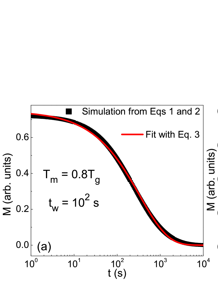
Figure 1: (a) TRM curve calculated at $T_{m}$ = 0.8$T_{g}$ with $H=A=c=1$ (arb. units) and $t_{w}$ = 100 s. The red solid line represents the best fit with Eq. 3. (b) Comparison of TRM curves calculated for different $t_{w}$. (c) The modulus of the relaxation rate $|S|$ for the TRM curves with different $t_{w}$. (d) $t_{cool}$ = 0 $TRM$ curves calculated with different $t_{w}$, plotted as a function of $t/t_{w}$. The inset compares the $|S|$ for $t_{w}$ = 100 s TRM curves calculated with $t_{cool}$ = 100 s and with $t_{cool}$ = 0.

For a quantitative comparison between the here proposed model and the one largely used to fit experimental TRM curves, the solid line in Fig. 1(a) shows a reasonably fit of Eq. 3 with the theoretical curve obtained from Eqs. 1 and LABEL:Eq2, yielding $t_{p}$ $\simeq$ 260 s, $n^{\prime}$ $\simeq$ 0.6, these values being within the range usually found for canonical SG Ocio . This clearly demonstrates that the proposed model is suitable to describe typical experimental TRM curves of SG materials. The fitting is not so good for small $t$, as was already observed experimentally at the early stages of investigation of SG systems, which motivated the search for alternative equations Ocio ; Chamberlin ; Nordblad . It is important to note the tendency toward zero in $M$, contrasting to the experimental results showing that usually the system reach a finite magnetization value at large $t$ Chamberlin ; Nordblad . It is thus possible that, in practice, for real SG materials a fraction of the spins gets pinned toward the $H$ direction after its removal, while the other part relax. This could be easily adjusted here with the addition of a constant term.

Fig. 1(b) compares TRM curves calculated for different $t_{w}$, where a clear $t_{w}$-dependence is observed. This is better visualized in Fig.1(c) where the modulus of the relaxation rate, $S=(1/H)(dM/dlnt)$, is computed. As can be seen, a maxima in $|S|$ occurs at $t$ close to $t_{w}$, again reproducing the experiments Nordblad . Such maxima is present even for $t_{w}$ = 0, which is due to the finite $t$ interval taken to cool the system from $T_{g}$ to $T_{m}$ ($t_{cool}$) Rodriguez ; Zotev ; Orbach . As $t_{w}$ increases, the relative influence of $t_{cool}$ diminishes and the maxima in $S$ gets closer to $t=t_{w}$. If one considers the situation in which the system is immediately cooled from above $T_{g}$ to $T_{m}$ (i.e. assuming an unrealistic $|dT/dt|=\infty$) then $t_{cool}=0$ and the peak in $S$ will shift to the left as shown in the inset of Fig. 1(d). Interestingly, all TRM curves calculated for $t_{cool}$ = 0 with different $t_{w}$, plotted as a function of $t/t_{w}$, coincide [Fig. 1(d)], in agreement with the tendency toward full aging experimentally found Rodriguez .

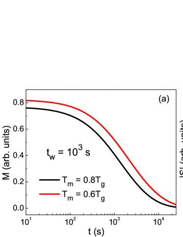
Figure 2: (a) Comparison between TRM curves obtained with $t_{w}$ = 10³ s and the same $H,a,c$, but distinct $T_{m}$. (b) The $|S|$ for these curves.

The model can faithfully predict the effect of thermal energy on the TRM curves. Fig. 2(a) compares the $t_{w}$ = 10³ s TRM curves obtained with $T$ = 0.8$T_{g}$ and 0.6$T_{g}$, where it is observed the increase in $M$ for the later, while Fig. 2(b) shows its expected $|S|$ shift to larger $t$ resulting from the fact that the spins get $more$ $freezed$ with decreasing $T$, turning the decay slower. In spite of the resemblance of Fig. 2(a) with that of the great majority of SG materials Chamberlin ; Nordblad , the $T$-dependence of $M_{0}$ expressed in Eq. LABEL:Eq2 is not expected to be universal, in the sense that there were also found materials for which the magnitude of $M$ decreases with $T$ Ocio . One can choose other $M_{0}(T)$ functions leading to different trends for the magnitude of $M$ as $T$ changes without greatly affecting the main SG features (see SM SM ).

II.2 Zero Field Cooled Magnetization

Besides the TRM experiments, the here proposed model can also reproduce the M_ZFC curves, which are obtained after ZFC the system down to $T_{m}$ $<$ $T_{g}$, keep it on this condition for $t_{w}$, then apply a small $H$ (at $t$ = 0) and start to capture $M$ as a function of $t$ (see SM SM ). Fig. 3(a) shows the curve calculated for $t_{w}$ = 10³ s at $T_{m}$ = 0.8$T_{g}$ and using the same parameters chosed to produce the TRM curves, i.e. $n$ = 0.5, $H=A=c=1$ (arb. units), resulting in a fair agreement with the typical experimental curves reported for SG system Lundgren . From a log-linear plot of the curves obtained with different $t_{w}$, Fig. 3(b), one can see the expected $t_{w}$-dependency observed experimentally Granberg . Fig. 3(c) displays the $S$ resulting from these M_ZFC curves. As for TRM, the maxima in $S$ for M_ZFC occurs at $t$ larger than (but close to) $t_{w}$, precisely the same behavior as that of experimental curves Granberg . Here, although there is no magnetization during cooling since it occurs at zero $H$, $t_{cool}$ still plays its part because according to Eq. LABEL:Eq2 the system starts to age already after the system passes through $T_{g}$ (at $t_{g}$). As $t_{w}$ increases, the relative effect of $t_{cool}$ decreases in comparison to $t_{w}$, and the maximum in $S$ gets closer to $t=t_{w}$. As in the case of TRM curves, if we assume $t_{cool}$ = 0 in the M_ZFC protocol the plot of $M$ as a function of $t/t_{w}$ will indicate a tendency toward full aging, Fig. 3(d). By comparing Figs. 1(c) and 3(c) quantitatively it can be noticed that, as observed experimentally, the relaxation rates of TRM and M_ZFC have nearly the same absolute values, indicating a similar aging process for both Sandlund .

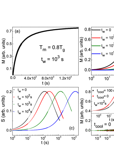
Figure 3: (a)M_ZFC curve calculated for $T_{m}$ = 0.8$T_{g}$, $n$ = 0.5, $H=A=c=1$ (arb.units) and $t_{w}$ = 10³ s. (b) Log-linear plots of the curves obtained with different $t_{w}$. (c) The relaxation rates, $S$, of the curves with different $t_{w}$. (d) M_ZFC curves calculated for $t_{cool}$ = 0 and different $t_{w}$, plotted as a function of $t/t_{w}$. The inset compares the $S$ of $t_{w}$ = 100 s M_ZFC curves calculated with $t_{cool}$ = 100 s and $t_{cool}$ = 0.

Another strategy developed to investigate the low $T$ dynamics of SG systems is the $T$ cycling below $T_{g}$. Fig. 4(a) shows the curve resulting from a protocol firstly proposed to investigate memory effects in assembly of magnetic nanoparticles Sun ; Khan , in which the system is ZFC down to $T_{m}$ $<$ $T_{g}$, then a small $H$ is applied (at $t$ = 0) and the magnetic relaxation starts to be captured. After the lapse of a period $t_{1}$, however, the system is further cooled to a lower $T$ = $T_{m}$ - $\Delta T$, and kept at this condition for a period $t_{2}$. After the lapse of $t_{2}$ the system is heated back to $T_{m}$ and the magnetization is recorded for a period $t_{3}$ SM .

The curve in Fig. 4(a) was produced with $T_{m}$ = 0.5$T_{g}$, $\Delta T$ = 0.2$T_{g}$, $t_{1}=t_{2}=t_{3}=4000$ s and the same parameter values as those used to calculate the conventional TRM and M_ZFC curves described above. At $t_{1}$ the curve is similar to those of Fig. 3, with an initial jump in the magnetization when $H$ is turned on, followed by a slow relaxation. During the temporary cooling at $t_{2}$, the relaxation becomes very weak, which can be inferred from the $T$-dependencies of Eqs. 1 and LABEL:Eq2. When the system returns to $T_{m}$ in $t_{3}$ the magnetization comes back to the level it reached before the $T$ cycling. The inset shows the curve resulting when the $t_{2}$ interval is removed. It makes clear the fact that during the temporary cooling the relaxation is almost halted, and the memory effect is manifested in $t_{3}$ when the system returns to $T_{m}$ and the relaxation is resumed, thus mimicking the experimental curves with precision Sun ; Khan . Conversely, for a positive $T$ cycling [Fig. 4(b)] the relaxation is hasted in $t_{2}$, and when the system is cooled back to $T_{m}$ the magnetization does not restore to the level reached before the temporary heating, also in agreement with experimental observations Sun ; Khan . These results indicate that the here proposed model may be also suitable for magnetic nanoparticles.

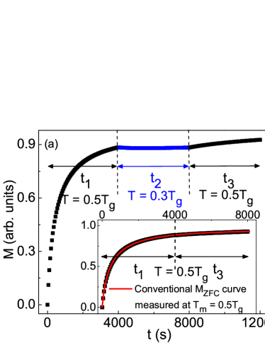
Figure 4: (a) M_ZFC curve calculated at $T_{m}$ = 0.5$T_{g}$ with a temporary cooling of $\Delta T$ = 0.2$T_{g}$. The inset shows the curve resulting when the data at $T_{m}$-$\Delta T$ is removed, evidencing the memory effect. (b) M_ZFC curve calculated at $T_{m}$ = 0.5$T_{g}$ with a temporary heating of $\Delta T$ = 0.2$T_{g}$, where no memory effects appear.

The model has failed, however, to reproduce the memory and rejuvenation effects for the case of M_ZFC experiments in which $T$ is cycled before the application of $H$ Nordblad2 , as well as the chaotic effect observed in the memory dip experiments where the ZFC process is halted prior to the measurement of M(T) Mathieu ; Jonason . It could not predict either the memory and rejuvenation effects in TRM experiments where $T$ is cycled during the measurement, because in this case $T$ is changed after the $H$ cutoff Sun ; Khan . For this last case, such contrast to the experiments suggests that the internal field may play an important role on the relaxation, and the here proposed model should be adjusted in order to take this into account. For instance, a natural attempt could be the replacement of $T(t^{\prime})$ by $T(t)$ in Eqs. 1 and LABEL:Eq2 since one may expect that, even in the absence of $H$, when $T$ is changed the energy landscape is altered and the decay will be affected (see SM SM ). This would lead to $T$ cycled TRM curves closer to the experimental ones, but would not reproduce the memory dip experiments.

II.3 Magnetization as a function of temperature

Finally, Eqs. 1 and LABEL:Eq2 can also predict the behavior of SG systems in ac and dc M(T) experiments. Fig. 5(a) shows the dc ZFC and FC curves calculated for $n$ = 0.5, $H=A=c=1$ (arb. units) and $|dT/dt|$ = 0.001 $T_{g}$/s. Despite the well known deviation from the Curie-Weiss (CW) behavior for the paramagnetic (PM) region of SG systems Morgownik , for simplicity it was chosen here a CW curve for the $T>T_{g}$ region, which was adjusted to coincide with the $T<T_{g}$ ZFC and FC curves at $T_{g}$. The ZFC curve shows a sharp cusp while the FC one shows a plateau-like behavior, being these striking features of SG systems Nagata . It is important to notice that the here proposed model does not predict the PM-SG transition, since it is only concerned with the SG state, $T<T_{g}$. The cusp-like behavior observed in Fig. 5 results from the fact the SG curves were calculated up to $T_{g}$ and joined to the PM ones that were calculated only down to this critical $T$. Concerning the fact that the experimental ZFC peaks are usually sharper than that of Fig. 5(a) while the FC ones usually show a small bump close to $T_{g}$, it must be stressed that the physics for $T$ very close to $T_{g}$, where a divergent behavior is expected, is neither under consideration here.

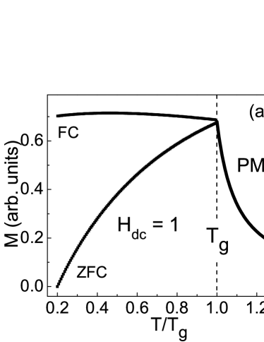
Figure 5: (a) ZFC and FC $dc$ M(T) curves calculated with $H$ = 1. (b) ac $\chi(T)$ curves calculated for $f$ = 0.1, 0.2 and 1 Hz.

According to the here proposed model, the ZFC curve depends on the cooling/heating $T$ rates (see SM SM ), as expected for an off-equilibrium condition Mydosh . Contrastingly, the FC is nearly invariant under changes in $|dT/dt|$ and this may be the reason why it is widely believed that the FC is roughly an equilibrium situation Malozemoff ; Chamberlin2 ; Matsui . However, it is in fact a metastable configuration Beckman , which can be fairly captured by the here proposed model. According to the model, if the cooling is halted for a finite $t$ interval below $T_{g}$ for instance, the FC magnetization will change SM , as already observed experimentally Pal .

Fig. 5(b) shows ac susceptibility curves for some selected frequencies ($f$), obtained considering an oscillating field of the form $H(t)=H_{dc}+hcos(2\pi ft)$, where $h$ is the ac field amplitude. All curves were calculated in the heating mode with $n$ = 0.5, $h=H_{dc}=A=1$, and each point was recorded after one field cycle. The $f$ were chosen slow enough so that one can assume a nearly linear response of $M$ in relation to $H$ and use the approximation $\chi=M/H$. The stretched exponential term in Eq. 1 is expected to depend on $H$, thus for Fig. 5(b) it was used $c=|H(t)|$, but very similar curves are observed for a constant $c$ (see SM SM ). The PM curve was calculated with the same slope of that used for the dc field shown in Fig. 5(a), and adjusted to coincide with the $f$ = 0.01 Hz curve at $T_{g}$, assumed here as a nearly static situation. The resulting curves are clearly $f$-dependent, showing a tendency of decrease in magnitude with increasing $f$. Defining the freezing $T$ ($T_{f}$) as the point where each curve intercepts the PM curve, one can observe the expected shift of $T_{f}$ toward higher $T$ as $f$ increases. The relative shift $\delta T_{f}$ = $\Delta T_{f}/T_{f}(\Delta logf)$ Mulder can be computed, yielding in this case a $\delta T_{f}\simeq$ 0.003 within the range experimentally found for canonical SG Mydosh . Though, care must be taken with this result since it depends on the choice of the PM curve, which is known to deviate from CW behavior for SG systems Morgownik . Moreover, it may be also related to the underline physics around $T_{g}$ (not considered here), so that the $T_{f}$ values may be related to the systems’ behavior at both above and below $T_{g}$.

III CONCLUSIONS

In summary, the model here proposed, based on a stretched exponential decay of the magnetization after the application of $H$ for an infinitesimal $t$, can describe the striking features of TRM, M_ZFC, ac and dc ZFC-FC M(T) curves and some of the memory experiments. It does not answer all the questions, thus it must be regarded as an approximate model. Nevertheless, the fact that it can reproduce several of the main SG features is remarkable, and its thorough investigation may give important insights into its physical origin, resulting in a better understanding of the microscopic mechanism behind the glassy behavior. In principle it could be also applied to other complex systems after a suitable adjustment of the parameters.

IV ACKNOWLEDGMENTS

This work was supported by Conselho Nacional de Desenvolvimento Científico e Tecnológico (CNPq), Fundação de Amparo à Pesquisa do Estado de Goiás (FAPEG) and Coordenação de Aperfeiçoamento de Pessoal de Nível Superior (CAPES). The author thanks Wesley B. Cardoso for the computational help.

References

- (1) M. Mézard, G. Parisi, and M. A. Virasoro, Spin Glass Theory and Beyond (World Scientific, Singapore, 1987).
- (2) J. A. Mydosh, Rep. Prog. Phys. 78 (2015) 052501.
- (3) D. L. Stein and C. M. Newman, Spin Glasses and Complexity (Princeton University Press, Princeton, 2013).
- (4) W. L. McMillan, J. Phys. C 17 (1984) 3179.
- (5) D. S. Fisher and D. A. Huse, Phys. Rev. B 38 (1988) 386.
- (6) D. Sherrington and S. Kirkpatrick, Phys. Rev. Lett. 35 (1975) 1792.
- (7) G. Parisi, Phys. Rev. Lett. 43 (1979) 1754.
- (8) G. Parisi, J. Phys. A 13 (2008) 324002.
- (9) C. M. Newman and D. L. Stein, Phys. Rev. E 57 (1998) 1356.
- (10) B. A. Berg and W. Janke, Phys. Rev. Lett. 80 (1998) 4771.
- (11) M. Ocio, M. Alba, and J. Hammann, J. Physique Lett. 46 (1985) 23.
- (12) R. V. Chamberlin, G. Mozurkewich, and R. Orbach, Phys. Rev. Lett. 52 (1984) 867.
- (13) P. Nordblad, P. Svedlindh, L. Lundgren, and L. Sandlund, Phys. Rev. B 33 (1986) 645.
- (14) See Supplementary Material at ??? for details of the computational calculation, the protocol and the equations used to produce each curve, as well as some results not displayed in the main text.
- (15) G. F. Rodriguez, G.G. Kenning, and R. Orbach, Phys. Rev. Lett. 91 (2003) 037203.
- (16) V. S. Zotev, G. F. Rodriguez, G. G. Kenning, R. Orbach, E. Vincent, and J. Hammann, Phys. Rev. B 67 (2003) 184422.
- (17) G. F. Rodriguez, G. G. Kenning, and R. Orbach, Phys. Rev. B 88 (2013) 054302.
- (18) L. Lundgren, P. Svedlindh, P. Nordblad, and O. Beckman, Phys. Rev. Lett. 51 (1983) 911.
- (19) P. Granberg, L. Sandlund, P. Nordblad, P. Svedlindh, and L. Lundgren, Phys. Rev. B 38 (1988) 7097.
- (20) P. Nordblad, L. Lundgren and L. Sandlund, J. Magn. Magn. Mater. 54-57 (1) (1986) 185-186.
- (21) Y. Sun, M. B. Salamon, K. Garnier, and R. S. Averback, Phys. Rev. Lett. 91 (2003) 167206.
- (22) N. Khan, P. Mandal, and D. Prabhakaran, Phys. Rev. B 90 (2014) 024421.
- (23) P. Granberg, L. Lundgren, and P. Nordblad, J. Magn. Magn. Mater. 92 (1990) 228-232.
- (24) R. Mathieu, P. Jönsson, D. N. H. Nam, and P. Nordblad, Phys. Rev. B 63 (2001) 092401.
- (25) K. Jonason, E. Vincent, J. Hammann, J. P. Bouchaud, and P. Nordblad, Phys. Rev. Lett. 81 (1998) 3243.
- (26) A. F. J. Morgownik and J. A. Mydosh, Phys. Rev. B 24 (1981) 5277.
- (27) S. Nagata, P. H. Keesom, and H. R. Harrison, Phys. Rev. B 19 (1979) 1633.
- (28) A. P. Malozemoff and Y. Imry, Phys. Rev. B 24 (1981) 489.
- (29) R. V. Chamberlin, M. Hardiman, L. A. Turkevich, and R. Orbach, Phys. Rev. B 25 (1982) 6720.
- (30) M. Matsui, A. P. Malozemoff, R. J. Gambino, and L. Krusin-Elbaum, J. Appl. Phys. 57 (1985) 3389.
- (31) L. Lundgren, P. Svedlindh, and O. Beckman, Phys. Rev. B 26 (1982) 3990.
- (32) S. Pal, K. Kumar, A. Banerjee, S. B. Roy, and A. K. Nigam, Phys. Rev. B 101 (2020) 180402(R).
- (33) C. A. M. Mulder, A. J. van Duyneveldt, and J. A. Mydosh, Phys. Rev. B 23 (1981) 1384.