GradSign: Model Performance Inference with Theoretical Insights
Abstract
A key challenge in neural architecture search (NAS) is quickly inferring the predictive performance of a broad spectrum of neural networks to discover statistically accurate and computationally efficient ones. We refer to this task as model performance inference (MPI). The current practice for efficient MPI is gradient-based methods that leverage the gradients of a network at initialization to infer its performance. However, existing gradient-based methods rely only on heuristic metrics and lack the necessary theoretical foundations to consolidate their designs. We propose GradSign, an accurate, simple, and flexible metric for model performance inference with theoretical insights. A key idea behind GradSign is a quantity to analyze the sample-wise optimization landscape of different networks. Theoretically, we show that is an upper bound for both the training and true population losses of a neural network under reasonable assumptions. However, it is computationally prohibitive to directly calculate for modern neural networks. To address this challenge, we design GradSign, an accurate and simple approximation of using the gradients of a network evaluated at a random initialization state. Evaluation on seven NAS benchmarks across three training datasets shows that GradSign generalizes well to real-world neural networks and consistently outperforms state-of-the-art gradient-based methods for MPI evaluated by Spearman’s and Kendall’s Tau. Additionally, we have integrated GradSign into four existing NAS algorithms and show that the GradSign-assisted NAS algorithms outperform their vanilla counterparts by improving the accuracies of best-discovered networks by up to 0.3%, 1.1%, and 1.0% on three real-world tasks. Code is available at https://github.com/cmu-catalyst/GradSign
1 Introduction
As deep learning methods evolve, neural architectures have gotten progressively larger and more sophisticated (He et al., 2015; Ioffe & Szegedy, 2015; Krizhevsky et al., 2017; Devlin et al., 2019; Rumelhart et al., 1986; Srivastava et al., 2014; Kingma & Ba, 2017), making it increasingly challenging to manually design model architectures that can achieve state-of-the-art predictive performance. To alleviate this challenge, recent work has proposed several approaches to automatically discovering statistically accurate and computationally efficient neural architectures. The most common approach is neural architecture search (NAS), which explores a comprehensive search space of potential network architectures that use a set of predefined network modules as basic building blocks. Recent work shows that NAS is able to discover architectures that outperform human-designed counterparts (Liu et al., 2018a; Zoph & Le, 2016; Pham et al., 2018).
A key challenge in NAS is quickly assessing the predictive performance of a diverse set of candidate architectures to discover performant ones. We refer to this task as model performance inference (MPI). A straightforward approach to MPI is directly training each candidate architecture on a dataset until convergence and recording the achieved training loss and validation accuracy (Frankle & Carbin, 2018; Chen et al., 2020a; Liu et al., 2018a; Zoph & Le, 2016). Though accurate, this approach is computationally prohibitive and cannot scale to large networks or datasets.
The current practice to efficient MPI is gradient-based methods that leverage the gradient information of a network at initialization to infer its predictive performance (Lee et al., 2018; Wang et al., 2020; Tanaka et al., 2020). Compared to directly measuring the accuracy of candidate networks on a training dataset, gradient-based methods are computationally more efficient since they only require evaluating a mini-batch of gradients at initialization. However, existing gradient-based methods rely only on heuristic metrics and lack the necessary theoretical insights to consolidate their designs.
In this paper, we propose GradSign, a simple yet accurate metric for MPI with theoretical foundations. GradSign is inspired by analyzing the sample-wise optimization landscape of a network. GradSign takes as inputs a mini-batch of sample-wise gradients evaluated at a random initialization point and outputs a statistical evidence of a network that highly correlates to its well-trained predictive performance measured by accuracy on the entire dataset.
Prior theoretical results (Allen-Zhu et al., 2019) show that the optimization landscape of a randomly initialized network is nearly convex and semi-smooth for a sufficiently large neighborhood. To realize its potential for MPI, we generalize these results to sample-wise optimization landscapes and propose a quantity to measure the density of sample-wise local optima in the convex areas around a random initialization point. Additionally, we prove that both the training loss and generalization error of a network are proportionally upper bounded by under reasonable assumptions.
Based on our theoretical results, we design GradSign, an accurate and simple approximation of . Empirically, we show that GradSign can also generalize to realistic setups that may violate our assumptions. In addition, GradSign is efficient to compute and easy to implement as it uses only the sample-wise gradient information of a network at a random initialization point.
Extensive evaluation of GradSign on seven NAS benchmarks (i.e., NAS-Bench-101, NAS-Bench-201, and five design spaces of NDS) across three datasets (i.e., CIFAR-10, CIFAR-100, and ImageNet16-120) shows that GradSign consistently outperforms existing gradient-based methods in all circumstances. Furthermore, we have integrated GradSign into existing NAS algorithms and show that the GradSign-assisted variants of these NAS algorithms lead to more accurate architectures.
Contributions.
This paper makes the following contributions:
-
•
We provide a new perspective to view the overall optimization landscape of a network as a combination of sample-wise optimization landscapes. Based on this insight, we introduce a new quantity that provides an upper bound on both the training loss and generalization error of a network under reasonable assumptions.
-
•
To infer , we propose GradSign, an accurate and simple estimation of . GradSign enables fast and efficient MPI using only the sample-wise gradients of a network at initialization.
-
•
We empirically show that GradSign generalizes to modern network architectures and consistently outperforms existing gradient-based MPI methods. Additionally, GradSign can be directly integrated into a variety of NAS algorithms to discover more accurate architectures.
2 Related Work
2.1 Model Performance Inference
Table 1 summarizes existing approaches to inferring the statistical performance of neural architectures.
Sample-based methods assess the performance of a neural architecture by training it on a dataset. Though accurate, sample-based methods require a surrogate training procedure to evaluate each architecture. EconNAS (Zhou et al., 2020) mitigates the cost of training candidate architectures by reducing the number of training epochs, input dataset sizes, resolution of input images, and model sizes.
Theory-based methods leverage recent advances in deep learning theory, such as Neural Tangent Kernel (Jacot et al., 2018) and Linear Region Analysis (Serra et al., 2018), to assess the predictive performance of a network (Chen et al., 2020a; Mellor et al., 2021; Park et al., 2020). In particular, NNGP (Park et al., 2020) infers a network’s performance by fitting its kernel regression parameters on a training dataset and evaluating its accuracy on a validation set, which alleviates the burden of training. As another example, Chen et al. (2020a) utilizes the kernel condition number proposed in Xiao et al. (2020), which can be theoretically proved to correlate to training convergence rate and generalization performance. However, this theoretical evidence is only guaranteed for extremely wide networks with a specialized initialization mode. While the linear region analysis used in Mellor et al. (2021), Lin et al. (2021) and Chen et al. (2020a) is easy to implement, such technique is only applicable to networks with ReLU activations (Agarap, 2018).
Learning-based methods train a separate network (e.g., graph neural networks) to predict a network’s accuracy (Liu et al., 2018a; Luo et al., 2020; Dai et al., 2019; Wen et al., 2020; Chen et al., 2020b; Siems et al., 2020). Though these learned models can achieve high accuracies on a specific task, this approach requires constructing a training dataset with sampled architectures for each downstream task. As a result, existing learning-based methods are generally task-specific and computationally prohibitive.
Gradient-based methods infer the statistical performance of a network by leveraging its gradient information at initialization, which can be easily obtained using an automated differentiation tool of today’s ML frameworks, such as PyTorch (Paszke et al., 2017) and TensorFlow (Abadi et al., 2016). The weight-wise salience score computed by several pruning at initialization (Lee et al., 2018; Wang et al., 2020; Tanaka et al., 2020) methods can easily be adapted to MPI settings by summing scores up. Though lack of theoretical foundations, such migrations have been empirically proven to be effective as baselines in recent works (Abdelfattah et al., 2021a; Mellor et al., 2021; Lin et al., 2021). An alternative stream of work (Turner et al., 2019; 2021; Theis et al., 2018) uses approximated second-order gradients, known as empirical Fisher Information Matrix (FIM), at a random initialization point to infer the performance of a network. Empirical FIM (Martens, 2014) is a valid approximation of a model’s predictive performance only if the model’s parameters are a Maximum Likelihood Estimation (MLE). However, this assumption is invalid at a random initialization point, making FIM-based algorithms inapplicable. A key difference between GradSign and existing gradient-based methods is that GradSign is based on a fine-grained analysis of sample-wise optimization landscapes rather than heuristic insights. In addition, GradSign also provides the first attempt for MPI by leveraging the optimization landscape properties contained in sample-wise gradient information, while prior gradient-based methods only focus on gradients evaluated in a full batch fashion.
| Methods | Theoretical | Training | Model | Task | |
| Insight | Free | Independent | Independent | ||
| Sample-Based | EconNAS | ✗ | ✗ | ✓ | ✓ |
| Theory-Based | NNGP, TE-NAS, | ✓ | ✓ | ✗ | ✓ |
| NASWOT, ZenNAS | |||||
| Learning-Based | Neural Predictor, | ✗ | ✗ | ✓ | ✗ |
| One-Shot-NAS-GCN | |||||
| Gradient-Based | Snip, Grasp, Synflow | ✗ | ✓ | ✓ | ✓ |
| Fisher | |||||
| GradSign (this paper) | ✓ | ✓ | ✓ | ✓ |
2.2 Neural Architecture Search
Recent work (He et al., 2021; Cai et al., 2019; 2018; Tan & Le, 2019; Howard et al., 2019) has proposed several algorithms to explore a NAS search space and discover highly accurate networks. RS (Bergstra & Bengio, 2012) is one of the baseline algorithms that generates and evaluates architectures randomly in the search space. REINFORCE (Williams, 1992) moves a step forward by reframing NAS as a reinforcement learning task where accuracy is the reward and architecture generation is the policy action. Given limited computational resources, BOHB (Falkner et al., 2018) uses Bayesian Optimization (BO) to propose candidates while uses HyperBand(HB) (Li et al., 2017) for searching resource allocation. REA (Real et al., 2019) uses a simple yet effective evolutionary searching strategy that achieves state-of-the-art performance. GradSign is complementary to and can be combined with existing NAS algorithms. We integrate GradSign into the NAS algorithms mentioned above and show that GradSign can consistently assist these NAS algorithms to discover more accurate architectures on various real-world tasks.
2.3 Optimization Landscape Analysis
Inspired by the fact that over-parameterized networks always find a remarkable fit for a training dataset (Zhang et al., 2016), optimization landscape analysis has been one of the main focuses in deep learning theory (Brutzkus & Globerson, 2017; Du et al., 2018; Ge et al., 2017; Li & Yuan, 2017; Soltanolkotabi, 2017; Allen-Zhu et al., 2019). Even though existing theoretical results for optimization landscape analysis rely on strict assumptions on the landscape’s smoothness, convexity, and initialization point, we can leverage theoretical insights to guide the design of GradSign. In addition, SGD-based optimizers trained from randomly initialized points hardly encounter non-smoothness or non-convexity in practice for a variety of architectures (Goodfellow et al., 2014). Furthermore, Allen-Zhu et al. (2019) provides theoretical evidence that for a sufficiently large neighborhood of a randomly initialized point, the optimization landscape is nearly convex and semi-smooth. Different from existing optimization landscape analyses depending on objectives evaluated across a mini-batch of training samples, we propose a new perspective that decomposes a mini-batch objective into the aggregation of sample-wise optimization landscapes. To the best of our knowledge, our work is the first attempt to MPI by leveraging sample-wise optimization landscapes.
3 Theoretical Foundations
3.1 Insights
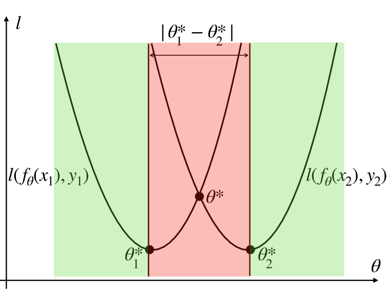
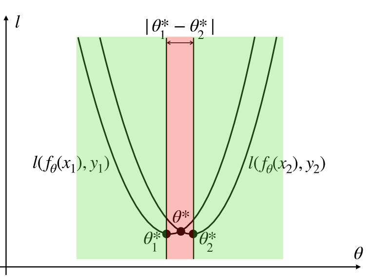
Conventional optimization landscape analyses focus on objectives across a mini-batch of training samples and miss potential evidence hidden in the optimization landscapes of individual samples. By decomposing a mini-batch objective into the summation of sample-wise objectives across individual samples in a mini-batch, we can distinguish better local optima as illustrated in Figure 1. Both Figure 1(a) and Figure 1(b) reach a local optimum at for the mini-batch objective . However, the optimization landscape in Figure 1(b) contains a better local optimum (i.e., a lower ). This can be distinguished by analyzing the relative distance between local optima across training samples (i.e., in Figure 1).
For a mini-batch with more than two samples, we use a sample-wise local optima density measurement defined in Section 3.2 to represent the overall closeness of sample-wise local optima. Intuitively, as the distances between the local optima across samples reduce (shown as the red areas in Figure 1), there is a higher probability that the gradients of different samples evaluated at a random initialization point have the same sign (shown as the green areas in Figure 1). Driven by this insight, we propose GradSign to infer the sample-wise local optima density statistically. The design of GradSign is based on our theoretical results that a network with denser sample-wise local optima has lower training and generalization losses under reasonable assumptions. We introduce the notations and assumptions in Section 3.2, provide a formal derivation of our theoretical results in Section 3.3, and present GradSign in Section 4.
3.2 Preliminaries
We use to denote training samples, where each is a feature vector, and is the corresponding label. We use to represent a loss function where is the prediction of our model. We use to denote the model parameterized by and use to denote random initialized parameters where is the number of model parameters. Bold font constant denotes a constant vector such as whose dimension depends on the corresponding situation. denotes the underline data distribution, which is the same for training and testing.
Our theoretical results rely on an assumption that there exists a neighborhood for a random initialization point in which sample-wise optimization landscapes are almost convex and semi-smooth. Note that our assumption is weaker than that of (Allen-Zhu et al., 2019) since their analysis is focusing on the overall optimization landscape while we only consider the sample-wise optimization landscape which is a simpler case. We use to denote a local optima in the convex areas attached to the -th sample near the initialization point . Under this assumption, the overall optimization landscape is also convex and semi-smooth within the neighborhood as additive operations preserve both. We use to denote a local optimum within for the mini-batch optimization landscape. Note that always lie in the convex hull of . Second, we assume that only gradient-based optimizers 111Gradient descent with infinitesimal step size are used during training. Thus the optimizer eventually converges to . Third, our theoretical analysis assumes that every Hessian in the set is almost diagonal as in the Neural Tangent Kernel (NTK) regime (Jacot et al., 2018). Section 5 shows that our method generalizes well to real-world networks that may violate this assumption.
Sample-wise local optima density. We use sample-wise local optima density to represent the relative closeness of . Given a dataset , an objective function , and a model class , we use to measure the average distance between the local optima across samples near a random initialization point :
| (1) |
is a smoothness upper bound: . This upper bound always exists due to the smoothness assumption. Intuitively, can be interpreted as the mean Manhattan distance with respect to each pair of normalized by the inverse of the square root of the smoothness upper bound. The denser are, the smaller is. In an ideal case, when all local optima are located at the same point.
3.3 Main Results
We show the local optimum property of sample-wise optimization landscapes in the following lemma.
Lemma 1
There exists no saddle point in a sample-wise optimization landscape and every local optimum is a global optimum.
Using Lemma 1, we can draw a relation between the training error and using the following theorem.
Theorem 2
The training error of a network on a dataset is upper bounded by , and the bound is tight when .
Finally, we show that also provides an upper bound for the generalization performance of a network measured by population loss.
Theorem 3
Given that is bounded by where is a local optimum attached to the convex area near for . With probability , the true population loss is upper bounded by .
A formal proof of all theoretical results is available in Section A.2.
Main takeaways: A key takeaway of our theoretical results is that closely relates to an upper bound of the training and generalization performance of a network. Albeit theoretically sound, is intractable to be directly measured. Instead, we derive a simple yet accurate metric to reflect , which we present in the next section.
4 GradSign
Inspired by the theoretical results derived above, we introduce GradSign, a simple yet accurate metric for model performance inference. The key idea behind GradSign is a quantity to statistically reflect the relative value of . Specifically,
| (2) |
where is a constant and is the vector index. Detailed derivation is given in Equation 25. Using the above relation, we can infer by directly measuring the signs of the gradients for a mini-batch of training samples at a randomly initialized point instead of going through an end-to-end training process.
To enable more efficient calculation of , we make a further simplification and use the following sample observation:
| (3) |
to infer the true probability whose relation is given by:
| (4) | |||||
| (5) |
The proof of this simplification is included in Equation 26. Given the above relationship, we formally state our algorithm pipeline in Algorithm 1. Note that a higher GradSign score indicates better model performance as we have an inverse correlation in Equation 2.
5 Experiments
In this section, we empirically verify the effectiveness of our metric against existing gradient-based methods on three neural architecture search (NAS) benchmarks, including NAS-Bench-101 (Ying et al., 2019), NAS-Bench-201 (Dong & Yang, 2020) and NDS (Radosavovic et al., 2019)222All datasets have consented for research purposes and no identifiable personal information is included.. Theory-based, sample-based, and learning-based methods are excluded in our evaluation, as they either require further training processes or have strong assumptions not suitable for generic architectures.
Baselines. We compare GradSign against existing gradient-based methods, including snip (Lee et al., 2018), grasp (Wang et al., 2020), fisher (Turner et al., 2019), and Synflow. In addition, we also include grad_norm as a heuristic method and a one-shot MPI metric NASWOT(Mellor et al., 2021). Since all gradient-based methods share a similar calculation pipeline (i.e., evaluating the gradients of a mini-batch at a random initialization point), we set the initialization mode and batch size to be the same across all methods to guarantee fairness. Experimental setup details are included in Section A.3. To align with the experimental setup of prior work (Abdelfattah et al., 2021b; Mellor et al., 2021), we use two criteria to evaluate the correlations between different metrics and test accuracies across approximately 20k networks:
Spearman’s (Daniel et al., 1990) characterizes the monotonic relationships between two variables. The correlation score is restricted in range [-1, 1], where denotes a perfect positive monotonic relationship and denotes a perfect negative monotonic relationship. Following prior work, we use Spearman’s to evaluate gradient-based methods on NAS-Bench-101 and NAS-Bench-201.
Kendall’s Tau. Similar to Spearman’s as a correlation measurement, Kendall’s Tau is also restricted between [-1, 1]. While Spearman’s is more sensitive to error and discrepancies, Kendall’s Tau is more robust with a smaller gross error sensitivity. We use Kendall’s Tau to quantify the correlation between one-shot metric scores and model testing accuracies over the NDS search space.
5.1 NAS-Bench-101
NAS-Bench-101 is the first dataset targeting large-scale neural architecture space, containing 423k unique convolutional architectures trained on the CIFAR-10 dataset. The benchmark provides the test accuracy of each architecture in the search space, which we use to calculate the corresponding Spearman’s . We use a randomly sampled subset with approximately architectures of the original search space and a batch size of 64 in this experiment. Table 2 summarizes the results. GradSign significantly outperforms existing gradient-based methods and heuristic approaches and improves the Spearman’s score by compared to the best existing method ().
| Dataset | grad_norm | snip | grasp | fisher | Synflow | NASWOT | GradSign |
|---|---|---|---|---|---|---|---|
| CIFAR10 | 0.263 | 0.189 | 0.315 | 0.3 | 0.363 | 0.324 | 0.449 |
5.2 NAS-Bench-201
NAS-Bench-201 is an extended version of NAS-Bench-101 with a different search space, containing 15,625 cell-based candidate architectures evaluated across three datasets: CIFAR-10, CIFAR-100 (Krizhevsky, 2009) and ImageNet 16-120 (Russakovsky et al., 2015). The benchmark provides the test accuracies on the three datasets for all candidate architectures in the search space. We evaluate Spearman’s scores for GradSign and existing gradient-based methods. The experiments were conducted overall 15,265 architectures in NAS-Bench-201. The batch size is set to 64. The results on the three datasets are summarized in Table 3. GradSign consistently achieves the best performance across all three datasets and improves the Spearman’s scores by over the best existing approaches. This improvement is significant as the more Spearman’s approaches , the more difficult it can be further improved.
| Dataset | ZenNAS | grad_norm | snip | grasp | fisher | Synflow | NASWOT | GradSign |
|---|---|---|---|---|---|---|---|---|
| CIFAR10 | -0.016 | 0.594 | 0.595 | 0.51 | 0.36 | 0.737 | 0.728 | 0.765 |
| CIFAR100 | -0.041 | 0.637 | 0.637 | 0.549 | 0.386 | 0.763 | 0.703 | 0.793 |
| ImageNet16-120 | 0.032 | 0.579 | 0.579 | 0.552 | 0.328 | 0.751 | 0.696 | 0.783 |
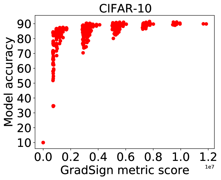
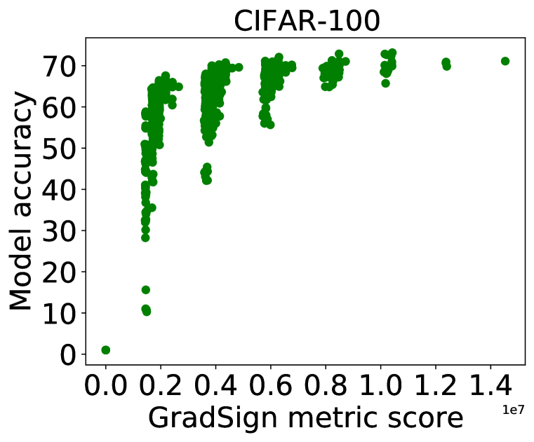
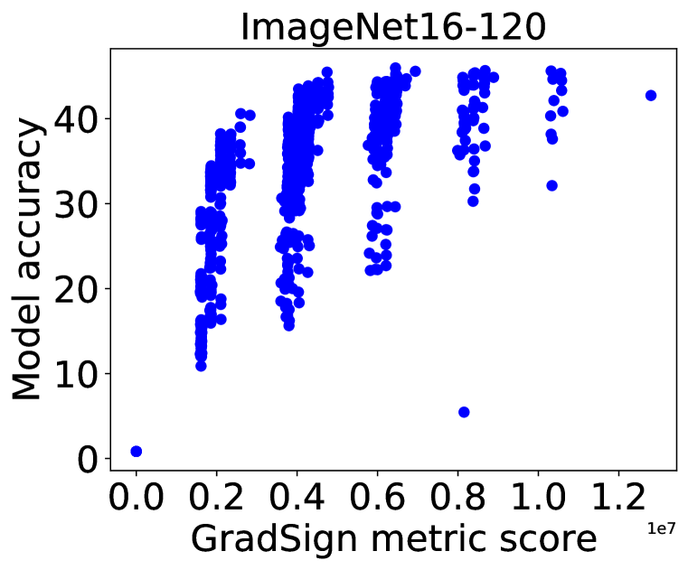
We further select 1000 architecture candidates randomly in the NAS-Bench-201 search space and visualize their testing accuracies against GradSign scores in Figure 2. Figure 2 shows a highly positive correlation between the GradSign score and actual test accuracy of 1000 architectures. A higher GradSign score indicates higher confidence for the statistical performance of architecture. Note that the GradSign scores show a clustering pattern, which may correspond to different architecture classes in the NAS-Bench-201 search space.
5.3 NAS Design Space (NDS)
NDS is a unified searching framework that includes five different design spaces: NAS-Net (Zoph et al., 2018), AmoebaNet (Real et al., 2019), PNAS (Liu et al., 2018a), ENAS (Pham et al., 2018), DARTS (Liu et al., 2018b). Each space contains approximately one thousand networks fully trained on the CIFAR-10 dataset. We include the performance of our method along with grad_norm, Synflow, and NASWOT on all five design spaces evaluated by Kendall’s Tau and show the results in Table 4. GradSign significantly and consistently outperforms all other MPI methods in all five design spaces.
| DARTS | ENAS | PNAS | NASNet | Amoeba | |
|---|---|---|---|---|---|
| grad_norm | 0.28 | -0.02 | -0.01 | -0.08 | -0.10 |
| Synflow | 0.37 | 0.02 | 0.03 | -0.03 | -0.06 |
| NASWOT | 0.48 | 0.34 | 0.31 | 0.31 | 0.20 |
| GradSign | 0.54 | 0.43 | 0.40 | 0.31 | 0.24 |
5.4 Architecture Selection
We evaluate whether GradSign can be directly used to select highly accurate architectures in a NAS search space. To pick a top architecture, we randomly sample candidates in a NAS search space, choose the one with the highest GradSign score, and measure its validation/test accuracies (meanstd). We compare GradSign with Synflow, NASWOT, Random, and Optimal, where Random uniformly samples architectures in the search space, while Optimal always chooses the best architecture across candidates. The results333the results for NASWOT are referenced from their paper (Mellor et al., 2021) are summarized in Table 5. in parenthesis indicates the number of architectures sampled in each run. All methods can generally find more accurate architectures with a high . In addition to outperforming Synflow and NASWOT, GradSign () can also find better networks even compared to NASWOT(). The results show that GradSign can directly identify accurate architectures besides highly correlating to networks’ test accuracies.
| Methods | CIFAR-10 | CIFAR-100 | ImageNet16-120 | |||
| Validation | Test | Validation | Test | Validation | Test | |
| Synflow(N=100) | 89.830.75 | 93.120.52 | 69.891.87 | 69.941.88 | 41.944.13 | 42.264.26 |
| NASWOT(N=100) | 89.550.89 | 92.810.99 | 69.351.70 | 69.481.70 | 42.813.05 | 43.103.16 |
| NASWOT(N=1000) | 89.690.73 | 92.960.81 | 69.981.22 | 69.861.21 | 44.442.10 | 43.952.05 |
| GradSign(N=100) | 89.840.61 | 93.310.47 | 70.221.32 | 70.331.28 | 42.072.78 | 42.422.81 |
| Random | 83.2013.28 | 86.6113.46 | 60.7012.55 | 60.8312.58 | 33.349.39 | 33.139.66 |
| Optimal(N=100) | 91.050.28 | 93.840.23 | 71.450.79 | 71.560.78 | 45.370.61 | 45.670.64 |
5.5 GradSign-Assisted Neural Architecture Search
Besides evaluating GradSign on the Spearman’s and Kendall’s Tau scores as prior work, we also integrate GradSign into various neural architecture search algorithms and evaluate how GradSign can assist neural architecture search on real-world tasks. Specifically, we integrate GradSign into four NAS algorithms: REA, REINFORCE, BOHB and RS. We design a corresponding method for each NAS algorithm that uses the GradSign scores of candidate architectures to guide the search. Specifically, we integrate GradSign into each NAS algorithm by replacing the random selection of architectures with GradSign-assisted selection. We name these GradSign-assisted variants G-REA, G-REINFROCE, G-HB, and G-RS, and describe their algorithm details in Appendix A.
To evaluate how GradSign can improve the search procedure of NAS algorithms, we run each algorithm with and without GradSign’s assistance for 500 runs on NAS-Bench-201 and report the validation and test accuracies of the best-discovered architecture in each run. Following prior work (Mellor et al., 2021; Dong & Yang, 2020), all searches are conducted on the CIFAR-10 dataset with a time budget of 12000s while the performance is evaluated on CIFAR-10, CIFAR-100 and ImageNet16-120. The baselines also include A-REA (Mellor et al., 2021), a variant of REA that uses the NASWOT scores at the initial population selection phase.
Table 6 shows the results. The GradSign-assisted NAS algorithms outperform their counterparts by improving test accuracy by up to 0.3%, 1.1%, and 1.0% on the three datasets.
| Methods | CIFAR-10 | CIFAR-100 | ImageNet16-120 | |||
| Validation | Test | Validation | Test | Validation | Test | |
| REA | 91.080.45 | 93.850.44 | 71.591.33 | 71.641.25 | 44.901.20 | 45.251.41 |
| A-REA | 91.200.27 | - | 71.950.99 | - | 45.701.05 | - |
| G-REA | 91.270.58 | 94.100.52 | 72.641.57 | 72.701.50 | 45.691.33 | 45.71.32 |
| RS | 90.930.37 | 93.720.38 | 70.961.12 | 71.071.07 | 44.471.08 | 44.611.22 |
| G-RS | 91.240.21 | 94.020.21 | 72.150.77 | 72.200.76 | 45.380.79 | 45.770.79 |
| REINFORCE | 90.320.89 | 93.210.82 | 70.031.75 | 70.141.73 | 43.572.09 | 43.642.24 |
| G-REINFORCE | 90.470.55 | 93.370.47 | 70.001.20 | 70.201.29 | 44.331.25 | 44.051.48 |
| BOHB | 90.840.49 | 93.640.49 | 70.821.29 | 70.921.26 | 44.361.37 | 44.501.50 |
| G-HB | 91.180.26 | 93.960.25 | 71.920.92 | 71.990.85 | 45.290.84 | 45.530.92 |
6 Conclusion
In this paper, we propose a model performance inference metric GradSign and provide theoretical foundations to support our metric. Instead of focusing on full batch optimization landscape analysis, we move a step further to sample-wise optimization landscape properties, which give us additional information to uncover the quality of the local optima encountered on the optimization trajectory. We propose to quantitatively characterize the potential of a model at a random initialization point based on our theory results. Finally, we design the GradSign metric to statistically infer the value of to give out our final score for model performance inference. Empirically, we have demonstrated that our method consistently achieves the best correlation with true model performance among all other gradient-based metrics. In addition, we also verified the practical value of our method in assisting existed NAS algorithms to achieve better results. Given that our metric is generic and promising, we believe that our work not only assists in accelerating MPI-related applications but sheds some light on optimization landscape analysis as well. Meanwhile, the effectiveness of our method may further reduce the energy cost introduced by modern NAS algorithms. In addition, one of the future work of GradSign can be adding normalization across different architecture classes to tackle the clustering problem in Figure 2.
References
- Abadi et al. (2016) Martín Abadi, Paul Barham, Jianmin Chen, Zhifeng Chen, Andy Davis, Jeffrey Dean, Matthieu Devin, Sanjay Ghemawat, Geoffrey Irving, Michael Isard, et al. Tensorflow: A system for large-scale machine learning. In 12th USENIX symposium on operating systems design and implementation (OSDI 16), pp. 265–283, 2016.
- Abdelfattah et al. (2021a) Mohamed S Abdelfattah, Abhinav Mehrotra, Łukasz Dudziak, and Nicholas D Lane. Zero-cost proxies for lightweight nas. arXiv preprint arXiv:2101.08134, 2021a.
- Abdelfattah et al. (2021b) Mohamed S. Abdelfattah, Abhinav Mehrotra, Łukasz Dudziak, and Nicholas D. Lane. Zero-Cost Proxies for Lightweight NAS. In International Conference on Learning Representations (ICLR), 2021b.
- Agarap (2018) Abien Fred Agarap. Deep learning using rectified linear units (relu). arXiv preprint arXiv:1803.08375, 2018.
- Allen-Zhu et al. (2019) Zeyuan Allen-Zhu, Yuanzhi Li, and Zhao Song. A convergence theory for deep learning via over-parameterization. In International Conference on Machine Learning, pp. 242–252. PMLR, 2019.
- Bergstra & Bengio (2012) James Bergstra and Yoshua Bengio. Random search for hyper-parameter optimization. Journal of machine learning research, 13(2), 2012.
- Brutzkus & Globerson (2017) Alon Brutzkus and Amir Globerson. Globally optimal gradient descent for a convnet with gaussian inputs. In International conference on machine learning, pp. 605–614. PMLR, 2017.
- Cai et al. (2018) Han Cai, Ligeng Zhu, and Song Han. Proxylessnas: Direct neural architecture search on target task and hardware. arXiv preprint arXiv:1812.00332, 2018.
- Cai et al. (2019) Han Cai, Chuang Gan, Tianzhe Wang, Zhekai Zhang, and Song Han. Once-for-all: Train one network and specialize it for efficient deployment. arXiv preprint arXiv:1908.09791, 2019.
- Chen et al. (2020a) Tianlong Chen, Jonathan Frankle, Shiyu Chang, Sijia Liu, Yang Zhang, Zhangyang Wang, and Michael Carbin. The lottery ticket hypothesis for pre-trained bert networks. arXiv preprint arXiv:2007.12223, 2020a.
- Chen et al. (2020b) Xin Chen, Lingxi Xie, Jun Wu, Longhui Wei, Yuhui Xu, and Qi Tian. Fitting the search space of weight-sharing nas with graph convolutional networks. arXiv preprint arXiv:2004.08423, 2020b.
- Dai et al. (2019) Xiaoliang Dai, Peizhao Zhang, Bichen Wu, Hongxu Yin, Fei Sun, Yanghan Wang, Marat Dukhan, Yunqing Hu, Yiming Wu, Yangqing Jia, et al. Chamnet: Towards efficient network design through platform-aware model adaptation. In Proceedings of the IEEE/CVF Conference on Computer Vision and Pattern Recognition, pp. 11398–11407, 2019.
- Daniel et al. (1990) Wayne W Daniel et al. Applied nonparametric statistics. 1990.
- Devlin et al. (2019) Jacob Devlin, Ming-Wei Chang, Kenton Lee, and Kristina Toutanova. Bert: Pre-training of deep bidirectional transformers for language understanding, 2019.
- Dong & Yang (2020) Xuanyi Dong and Yi Yang. Nas-bench-201: Extending the scope of reproducible neural architecture search. arXiv preprint arXiv:2001.00326, 2020.
- Du et al. (2018) Simon Du, Jason Lee, Yuandong Tian, Aarti Singh, and Barnabas Poczos. Gradient descent learns one-hidden-layer cnn: Don’t be afraid of spurious local minima. In International Conference on Machine Learning, pp. 1339–1348. PMLR, 2018.
- Falkner et al. (2018) Stefan Falkner, Aaron Klein, and Frank Hutter. Bohb: Robust and efficient hyperparameter optimization at scale. In International Conference on Machine Learning, pp. 1437–1446. PMLR, 2018.
- Frankle & Carbin (2018) Jonathan Frankle and Michael Carbin. The lottery ticket hypothesis: Finding sparse, trainable neural networks. arXiv preprint arXiv:1803.03635, 2018.
- Ge et al. (2017) Rong Ge, Jason D Lee, and Tengyu Ma. Learning one-hidden-layer neural networks with landscape design. arXiv preprint arXiv:1711.00501, 2017.
- Goodfellow et al. (2014) Ian J Goodfellow, Oriol Vinyals, and Andrew M Saxe. Qualitatively characterizing neural network optimization problems. arXiv preprint arXiv:1412.6544, 2014.
- He et al. (2015) Kaiming He, Xiangyu Zhang, Shaoqing Ren, and Jian Sun. Deep residual learning for image recognition, 2015.
- He et al. (2021) Xin He, Kaiyong Zhao, and Xiaowen Chu. Automl: A survey of the state-of-the-art. Knowledge-Based Systems, 212:106622, 2021.
- Howard et al. (2019) Andrew Howard, Mark Sandler, Grace Chu, Liang-Chieh Chen, Bo Chen, Mingxing Tan, Weijun Wang, Yukun Zhu, Ruoming Pang, Vijay Vasudevan, Quoc V. Le, and Hartwig Adam. Searching for mobilenetv3. In Proceedings of the IEEE/CVF International Conference on Computer Vision (ICCV), October 2019.
- Ioffe & Szegedy (2015) Sergey Ioffe and Christian Szegedy. Batch normalization: Accelerating deep network training by reducing internal covariate shift, 2015.
- Jacot et al. (2018) Arthur Jacot, Franck Gabriel, and Clément Hongler. Neural tangent kernel: Convergence and generalization in neural networks. arXiv preprint arXiv:1806.07572, 2018.
- Kingma & Ba (2017) Diederik P. Kingma and Jimmy Ba. Adam: A method for stochastic optimization, 2017.
- Krizhevsky (2009) Alex Krizhevsky. Learning multiple layers of features from tiny images. Technical report, 2009.
- Krizhevsky et al. (2017) Alex Krizhevsky, Ilya Sutskever, and Geoffrey E. Hinton. Imagenet classification with deep convolutional neural networks. Communications of the ACM, 60(6):84–90, 5 2017. ISSN 1557-7317. doi: 10.1145/3065386. URL http://dx.doi.org/10.1145/3065386.
- Lee et al. (2018) Namhoon Lee, Thalaiyasingam Ajanthan, and Philip HS Torr. Snip: Single-shot network pruning based on connection sensitivity. arXiv preprint arXiv:1810.02340, 2018.
- Li et al. (2017) Lisha Li, Kevin Jamieson, Giulia DeSalvo, Afshin Rostamizadeh, and Ameet Talwalkar. Hyperband: A novel bandit-based approach to hyperparameter optimization. The Journal of Machine Learning Research, 18(1):6765–6816, 2017.
- Li & Yuan (2017) Yuanzhi Li and Yang Yuan. Convergence analysis of two-layer neural networks with relu activation. arXiv preprint arXiv:1705.09886, 2017.
- Lin et al. (2021) Ming Lin, Pichao Wang, Zhenhong Sun, Hesen Chen, Xiuyu Sun, Qi Qian, Hao Li, and Rong Jin. Zen-nas: A zero-shot nas for high-performance image recognition. In Proceedings of the IEEE/CVF International Conference on Computer Vision, pp. 347–356, 2021.
- Liu et al. (2018a) Chenxi Liu, Barret Zoph, Maxim Neumann, Jonathon Shlens, Wei Hua, Li-Jia Li, Li Fei-Fei, Alan Yuille, Jonathan Huang, and Kevin Murphy. Progressive neural architecture search. In Proceedings of the European conference on computer vision (ECCV), pp. 19–34, 2018a.
- Liu et al. (2018b) Hanxiao Liu, Karen Simonyan, and Yiming Yang. Darts: Differentiable architecture search. arXiv preprint arXiv:1806.09055, 2018b.
- Luo et al. (2020) Renqian Luo, Xu Tan, Rui Wang, Tao Qin, Enhong Chen, and Tie-Yan Liu. Semi-supervised neural architecture search. arXiv preprint arXiv:2002.10389, 2020.
- Martens (2014) James Martens. New insights and perspectives on the natural gradient method. arXiv preprint arXiv:1412.1193, 2014.
- Mellor et al. (2021) Joseph Mellor, Jack Turner, Amos Storkey, and Elliot J. Crowley. Neural architecture search without training, 2021.
- Ning et al. (2020) Xuefei Ning, Yin Zheng, Tianchen Zhao, Yu Wang, and Huazhong Yang. A generic graph-based neural architecture encoding scheme for predictor-based nas. In Computer Vision–ECCV 2020: 16th European Conference, Glasgow, UK, August 23–28, 2020, Proceedings, Part XIII 16, pp. 189–204. Springer, 2020.
- Park et al. (2020) Daniel S Park, Jaehoon Lee, Daiyi Peng, Yuan Cao, and Jascha Sohl-Dickstein. Towards nngp-guided neural architecture search. arXiv preprint arXiv:2011.06006, 2020.
- Paszke et al. (2017) Adam Paszke, Sam Gross, Soumith Chintala, Gregory Chanan, Edward Yang, Zachary DeVito, Zeming Lin, Alban Desmaison, Luca Antiga, and Adam Lerer. Automatic differentiation in pytorch. 2017.
- Pham et al. (2018) Hieu Pham, Melody Guan, Barret Zoph, Quoc Le, and Jeff Dean. Efficient neural architecture search via parameters sharing. In International Conference on Machine Learning, pp. 4095–4104. PMLR, 2018.
- Radosavovic et al. (2019) Ilija Radosavovic, Justin Johnson, Saining Xie, Wan-Yen Lo, and Piotr Dollár. On network design spaces for visual recognition. In Proceedings of the IEEE/CVF International Conference on Computer Vision, pp. 1882–1890, 2019.
- Real et al. (2019) Esteban Real, Alok Aggarwal, Yanping Huang, and Quoc V Le. Regularized evolution for image classifier architecture search. In Proceedings of the aaai conference on artificial intelligence, volume 33, pp. 4780–4789, 2019.
- Rumelhart et al. (1986) David E Rumelhart, Geoffrey E Hinton, and Ronald J Williams. Learning representations by back-propagating errors. nature, 323(6088):533–536, 1986.
- Russakovsky et al. (2015) Olga Russakovsky, Jia Deng, Hao Su, Jonathan Krause, Sanjeev Satheesh, Sean Ma, Zhiheng Huang, Andrej Karpathy, Aditya Khosla, Michael Bernstein, et al. Imagenet large scale visual recognition challenge. International journal of computer vision, 115(3):211–252, 2015.
- Serra et al. (2018) Thiago Serra, Christian Tjandraatmadja, and Srikumar Ramalingam. Bounding and counting linear regions of deep neural networks. In International Conference on Machine Learning, pp. 4558–4566. PMLR, 2018.
- Siems et al. (2020) Julien Siems, Lucas Zimmer, Arber Zela, Jovita Lukasik, Margret Keuper, and Frank Hutter. Nas-bench-301 and the case for surrogate benchmarks for neural architecture search. arXiv preprint arXiv:2008.09777, 2020.
- Soltanolkotabi (2017) Mahdi Soltanolkotabi. Learning relus via gradient descent. arXiv preprint arXiv:1705.04591, 2017.
- Srivastava et al. (2014) Nitish Srivastava, Geoffrey Hinton, Alex Krizhevsky, Ilya Sutskever, and Ruslan Salakhutdinov. Dropout: A simple way to prevent neural networks from overfitting. Journal of Machine Learning Research, 15(56):1929–1958, 2014. URL http://jmlr.org/papers/v15/srivastava14a.html.
- Tan & Le (2019) Mingxing Tan and Quoc Le. EfficientNet: Rethinking model scaling for convolutional neural networks. In Kamalika Chaudhuri and Ruslan Salakhutdinov (eds.), Proceedings of the 36th International Conference on Machine Learning, volume 97 of Proceedings of Machine Learning Research, pp. 6105–6114. PMLR, 09–15 Jun 2019. URL https://proceedings.mlr.press/v97/tan19a.html.
- Tanaka et al. (2020) Hidenori Tanaka, Daniel Kunin, Daniel LK Yamins, and Surya Ganguli. Pruning neural networks without any data by iteratively conserving synaptic flow. arXiv preprint arXiv:2006.05467, 2020.
- Theis et al. (2018) Lucas Theis, Iryna Korshunova, Alykhan Tejani, and Ferenc Huszár. Faster gaze prediction with dense networks and fisher pruning. arXiv preprint arXiv:1801.05787, 2018.
- Turner et al. (2019) Jack Turner, Elliot J Crowley, Michael O’Boyle, Amos Storkey, and Gavin Gray. Blockswap: Fisher-guided block substitution for network compression on a budget. arXiv preprint arXiv:1906.04113, 2019.
- Turner et al. (2021) Jack Turner, Elliot J Crowley, and Michael FP O’Boyle. Neural architecture search as program transformation exploration. In Proceedings of the 26th ACM International Conference on Architectural Support for Programming Languages and Operating Systems, pp. 915–927, 2021.
- Wang et al. (2020) Chaoqi Wang, Guodong Zhang, and Roger Grosse. Picking winning tickets before training by preserving gradient flow. arXiv preprint arXiv:2002.07376, 2020.
- Wang et al. (2019) Linnan Wang, Yiyang Zhao, Yuu Jinnai, Yuandong Tian, and Rodrigo Fonseca. Alphax: exploring neural architectures with deep neural networks and monte carlo tree search. arXiv preprint arXiv:1903.11059, 2019.
- Wen et al. (2020) Wei Wen, Hanxiao Liu, Yiran Chen, Hai Li, Gabriel Bender, and Pieter-Jan Kindermans. Neural predictor for neural architecture search. In European Conference on Computer Vision, pp. 660–676. Springer, 2020.
- Williams (1992) Ronald J Williams. Simple statistical gradient-following algorithms for connectionist reinforcement learning. Machine learning, 8(3):229–256, 1992.
- Xiao et al. (2020) Lechao Xiao, Jeffrey Pennington, and Samuel Schoenholz. Disentangling trainability and generalization in deep neural networks. In International Conference on Machine Learning, pp. 10462–10472. PMLR, 2020.
- Ying et al. (2019) Chris Ying, Aaron Klein, Eric Christiansen, Esteban Real, Kevin Murphy, and Frank Hutter. Nas-bench-101: Towards reproducible neural architecture search. In International Conference on Machine Learning, pp. 7105–7114. PMLR, 2019.
- Zhang et al. (2016) Chiyuan Zhang, Samy Bengio, Moritz Hardt, Benjamin Recht, and Oriol Vinyals. Understanding deep learning requires rethinking generalization. arXiv preprint arXiv:1611.03530, 2016.
- Zhou et al. (2020) Dongzhan Zhou, Xinchi Zhou, Wenwei Zhang, Chen Change Loy, Shuai Yi, Xuesen Zhang, and Wanli Ouyang. Econas: Finding proxies for economical neural architecture search. In Proceedings of the IEEE/CVF Conference on Computer Vision and Pattern Recognition, pp. 11396–11404, 2020.
- Zoph & Le (2016) Barret Zoph and Quoc V Le. Neural architecture search with reinforcement learning. arXiv preprint arXiv:1611.01578, 2016.
- Zoph et al. (2018) Barret Zoph, Vijay Vasudevan, Jonathon Shlens, and Quoc V Le. Learning transferable architectures for scalable image recognition. In Proceedings of the IEEE conference on computer vision and pattern recognition, pp. 8697–8710, 2018.
Appendix A Appendix
A.1 Figure
A.2 Proof
Lemma 1 Proof: For a single training sample , we minimize its objective function with gradient descent:
| (6) |
At any local optimal point , we have , but for conventional neural architectures with at least one dense layer 444The gradient values corresponding to the bias term of the last dense layer are always non-zero.. Therefore, we show must be equal to . For the commonly used objective functions, such as Mean Squared Error Loss and Cross Entropy Loss, this derivative is equal to , where is a non-zero constant. Hence we have and at local optima , which makes also a global optima as it is impossible to obtain a lower loss value for this single sample. In addition, at local optima , we have:
| (7) | |||||
| (8) | |||||
| (9) |
The above equation implies that is a positive semi-definite matrix, since .
This concludes the proof of non existence of saddle points in a sample-wise optimization landscape. This result aligns with our convexity assumptions in Section 3.2.
Theorem 2 Proof: Recall that denotes a local optima of which could be reached by a gradient-flow based optimizer start from . Since is randomly sampled and , we have:
| (10) | |||||
| (11) | |||||
| (12) | |||||
| (13) | |||||
| (14) |
where Eq 10 Eq 11 uses the basic property of the smoothness upper bound and the fact that each local optimum satisfies . Eq 11 Eq 12 uses Jensen Inequality for square root operators. Eq 12 Eq 13 is derived from the fact that for each dimension in we have:
| (15) |
Otherwise, dose not lie in the convex hull of which contradicts with our assumption stated in Section 3.2. The bound is tight when .
Theorem 3 Proof: Let denotes the true population error. With probability , we have:
| (18) | |||||
| (19) | |||||
| (20) |
where and are constants, is a training dataset, and denotes its underlying data distribution. This implies that is an accurate indicator for the true population loss. Eq 18 Eq 19 uses Chebyshev’s inequality, while Eq 19 Eq 20 uses the same inequality derived in Claim 2.
Algorithm Proof: Given that sample-wise local optima are contained in the convex area around . We derive the following property:
| (21) |
Since is a randomly chosen initialization point, without loss of generality, we assume is sampled from a hypercube . Thus we have:
| (22) |
Where denotes the probability for and having different signs. Notice that we have completely dropped the dependency for at this point and can simply infer from . To complete our proof:
| (23) | |||||
| (24) | |||||
| (25) |
Simplification Proof:: for each and a given , we could estimate using:
| (26) |
which is valid (not equal to zero) only when . Suppose we have p positive and n-p negative for n samples, since we only care about samples share the same sign, the original probability estimation is . Thus we only need to measure the quantity which simply equals to .
A.3 Experiments Setup
The code we used during experimentation was mainly based on existed code base Abdelfattah et al. (2021b); Mellor et al. (2021)Abdelfattah et al. (2021b) which is under Apache-2.0 License.
The hardwares we used were Amazon EC2 C5 instances with no GPU involved and p3 instance with one V100 Tensor Core GPU.
As our methods is gradient-based which is training free, we don’t need to split our dataset. For Spearman’s correlation measurement on NAS-Bench-201, we set batch size to 64, which is used by most baselines. For the Kendall’s Tau experiment, other accuracy comparison experience and the GradSign assisted algorithms, we used a batch size of 128, also to match the batch size in other baselines (NASWOT). We use Pytorch default parameter initialization for all architectures. Random seed in correlation experiments is set to 42 which is also randomly chosen. For accuracy experiments, our results are summarized over 500 runs whose random seed are chosen randomly for each run. For the correlation evaluation of each individual architecture, we only use one for minimizing computational cost. Our approach can be easily generalized to an average of multiple s and can trade-off between efficiency and accuracy.
A.4 Additional results
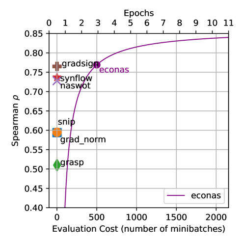
Sample-based: Fig 3 compares EconNAS, a sample-based method, with existing gradient-based methods on MPI. Results of EconNAS are referenced from Abdelfattah et al. (2021b). To achieve a similar MPI performance as GradSign, EconNAS needs 500 minibatches of samples for each candidate’s proxy training, while all gradient-based methods (including GradSign) require only one minibatch. By increasing the number of minibatches, EconNAS can achieve higher Spearman’s scores, which eventually converge to 0.85. At that point overfitting takes place and the score cannot be further improved.
Learning-based: Table 7 compares GradSign and existing learning-based methods (MLP, LSTM, and GATES) on the Kendall’s Tau correlation score. The MLP, LSTM, and GATES results are referenced from Ning et al. (2020). For MLP and LSTM (Wang et al., 2019), the predictor uses Multi Layer Perceptron (MLP) and Long Short Term Memory (LSTM) as the base predictor, while GATES (Ning et al., 2020) uses Graph Neural Network (GNN) as the base predictor. All results are obtained on NAS-Bench-201 and the GradSign’s score is averaged over all three datasets (CIFAR-10, CIFAR-100 and ImageNet16-120) as (Ning et al., 2020) does not provide which dataset is used for calculating Kendall’s Tau.
To achieve a similar score as GradSign, MLP, LSTM and GATES-1 require an average of 1959, 978 and 1959 minibatches per sample respectively to prepare the dataset for training the predictors. Although GATES-2 achieves a better correlation score than GradSign, it still needs 195 minibatches per sample to prepare the dataset for training the GATES-2 predictor. In addition to the cost of preparing a training dataset, each predictor also has to be trained on the dataset as well, which involves 200 more epochs while the cost of evaluating GradSign is one mini-batch. With less mini-batches evaluated for learning-based methods, their training set sizes shrink significantly (e.g., 195 mini-batches equal to 78 training samples and 7813 testing samples). This may result in overfitting to the training set.
| Kendall’s Tau | Average minibatches per sample | |
|---|---|---|
| MLP | 0.5388 | 1959 |
| LSTM | 0.6407 | 978 |
| GATES-1 | 0.45 | 1959 |
| GATES-2 | 0.7401 | 195 |
| GradSign | 0.6016 | 1 |
We also includes the evaluation of GradSign for both MPI correlation performance and GradSign-assisted NAS algorithms on the latest version of NAS-Bench-201 (NATS-Bench) across three datasets (CIFAR-10, CIFAR-100 and ImageNet16-120) in Table 8, Table 9. Results show GradSign is robust against hyper-parameter tuning as long as the trained networks can converge to near optimal. Also notice that GradSign-assisted NAS algorithms could not only achieve a better accuracy but lower variance as well compared to their non-assisted counterparts.
| CIFAR-10 | CIFAR-100 | ImageNet16-120 | |
|---|---|---|---|
| NAS-Bench-201 | 0.765 | 0.793 | 0.783 |
| NATS-Bench | 0.760 | 0.792 | 0.784 |
| Methods | CIFAR-10 | CIFAR-100 | ImageNet16-120 | |||
|---|---|---|---|---|---|---|
| Validation | Test | Validation | Test | Validation | Test | |
| REA | 91.060.49 | 93.840.45 | 71.531.31 | 71.601.27 | 44.821.23 | 45.181.37 |
| G-REA | 91.350.35 | 94.150.32 | 72.671.05 | 72.650.97 | 45.550.96 | 45.990.93 |
| RS | 90.950.28 | 93.770.26 | 71.010.97 | 71.150.95 | 44.580.95 | 44.731.10 |
| G-RS | 91.230.22 | 94.020.22 | 72.120.82 | 72.150.78 | 45.430.74 | 45.830.80 |
| REINFORCE | 90.920.38 | 93.710.37 | 71.041.02 | 71.171.12 | 44.560.97 | 44.801.18 |
| G-REINFORCE | 91.200.23 | 93.980.23 | 71.930.91 | 72.050.89 | 45.280.77 | 45.640.86 |
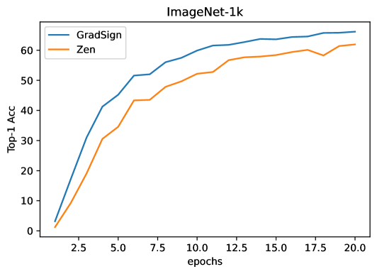
To demonstrate the potential for GradSign in a more complicated computer vision task, we compare the performance of GradSign with ZenNAS following their setups and search space. Due to the limitation of computational resources555the original setup in ZenNAS could take up to 8 months for training 480 epochs on ImageNet-1k, we only run 10000 evolution iterations using solely Zen score or GradSign score to select the architecture candidate and 20 epochs to train the selected architecture. Following ZenNAS’s setup, EfficientNet-B3 is used as teacher network when training selected architectures. Though the top-1 validation accuracy of GradSign in the first 20 epochs is slightly better than Zen, we should note that this process can highly depend on the random seed for evolution search phase. As we mentioned before, ZenNAS uses linear region analysis which makes it less flexible for arbitrary activation functions. On the other hand, since ZenNAS calculates an architecture complexity related score which is both dataset independent and initialization independent, it can be too general and results in low Spearman’s as shown in Table 3.