HD207897 b: A dense sub-Neptune transiting a nearby and bright K-type star

We present the discovery and characterization of a transiting sub-Neptune orbiting with a 16.20-day period around a nearby (28 pc) and bright (V= 8.37) K0V star HD207897 (TOI-1611). This discovery is based on photometric measurements from the Transiting Exoplanet Survey Satellite (TESS) mission and radial velocity (RV) observations from the SOPHIE, Automated Planet Finder (APF) and HIRES high precision spectrographs. We used EXOFASTv2 for simultaneously modeling the parameters of the planet and its host star, combining photometric and RV data to determine the planetary system parameters. We show that the planet has a radius of $2.50\pm 0.08$ R_E and a mass of either $14.4\pm 1.6$ M_E or $15.9\pm 1.6$ M_E with nearly equal probability; the two solutions correspond to two possibilities for the stellar activity period. Hence, the density is either $5.1\pm 0.7$ g cm^-3 or $5.5^{+0.8}_{-0.7}$ g cm^-3, making it one of the relatively rare dense sub-Neptunes. The existence of such a dense planet at only 0.12 AU from its host star is unusual in the currently observed sub-Neptune (2 ¡ R_E ¡ 4) population. The most likely scenario is that this planet has migrated to its current position.

1 Introduction

The brightness of more than 200,000 stars has been monitored by TESS (Ricker et al. 2015) with 2 minutes cadence during its two-year primary mission. The observed stars are closer and brighter (typically 30-100 times brighter) than the stars Kepler surveyed. This offers us a unique opportunity for furthering our knowledge in planetary science with follow-up observations: those from ground-based high precision spectrographs to confirm the planetary nature and mass measurement, which with the radius allows us to determine the bulk composition of planets; and ground and space-based observations to provide atmospheric characterization, for instance, with the upcoming James Webb Space Telescope (Gardner et al. 2006).

The NASA Kepler Mission (Borucki et al. 2010) has discovered a large number of planets of intermediate size, with radii between Earth and Neptune, also known as sub-Neptunes. Since the size of planets is directly dependent on physical mechanisms in formation and evolution, the absence of sub-Neptunes in our solar system and their abundance among the exoplanet population has raised numerous fundamental questions. Many theoretical and statistical studies have been made on such planets. Rogers (2015) showed that most planets with R ¿ 1.6 R_E have low density and are inconsistent with a pure rocky composition. Fulton et al. (2017) demonstrated that the sub-Neptunes’ distribution of radii is bimodal with 2 peaks centered at 1.2 R_E and 2.4 R_E, which reveals a gap in planet radii between 1.5–2.0 R_E. While this bi-modal distribution can be explained by photoevaporation (Owen & Wu 2013, 2017; Lopez & Fortney 2014) and core‐powered mass loss (Ginzburg et al. 2016, 2018) the composition and origin of close‐in sub‐Neptunes are not yet clear. Additional detections and precise characterizations are the keys to progress in answering our questions about their nature. One of the primary goals of TESS is to measure the mass of at least 50 transiting planets with a radius smaller than 4 Earth radii (Ricker et al. 2015). As of 22 April 2021, TESS has found more than 750 candidates (so-called TESS object of interest or TOI) with radii smaller than 4 R_E. To date, 122 of them have been confirmed and have a mass measurement (e.g., Dragomir et al. 2019; Günther et al. 2019; Nielsen et al. 2020).

Here, we announce the detection and characterization of a sub-Neptune orbiting a bright (V=8.4) K0 star using TESS photometric data and SOPHIE, APF, and HIRES RVs. In Sect. 2, we describe the variety of observations used to characterize the HD207897 (TOI-1611) system, including photometric, spectroscopic, and high-resolution imaging data. In Sect. 3, we analyze the data and present the characterization of the host star and planet, combining models on RVs and transit data. Finally, we present our discussion and conclude in Sect. 4.

2 Observations

2.1 Photometry

2.1.1 TESS

TESS planned to observe 80% of the sky in 26 sectors for 2 years. Each sector is approximately 27 days, with partial overlap between sectors . Because HD207897 is located near the north ecliptic pole where sectors overlap, it appears in many sectors. As reported in the Web TESS Viewing Tool (WTV), HD207897 observations were taken on five sectors divided into two continuous periods from sectors 18-20 and 25-26, with a total time span of 131 days. After observations of sector 18 were completed, the MIT’s Quick Look pipeline (QLP- Huang et al. 2020a, b) detected the signature of two transits of HD207897 b at a period of 16.20 d, and an alert was issued 19 December 2019 by the TESS Science Office. No transits occurred during sector 19 as the sole transit fell in the data gap between the two orbits. After observations of sector 20 were downlinked, the Science Processing Operations Center (SPOC; Jenkins et al. 2016) at NASA Ames Research Center conducted a transit search (Jenkins 2002; Jenkins et al. 2010) and detected two transits of HD207897 b at a signal-to-noise ratio (S/N) of 23.3. A limb-darkened transit model was fitted to the transit signature (Li et al. 2019), which passed all the diagnostic tests presented in the Data Validation report (Twicken et al. 2018), including the odd-even transit depth test, the ghost diagnostic test, and the difference image centroiding test, which located the source of the transit signatures within 0.42$\pm$2.5 arcsec of the target star HD207897. Two additional transits were observed and detected in sector 25, and one more occurred during sector 26. A multi-sector search of sectors 18-26 by the SPOC detected 7 transit events of HD207897 b in total, at an S/N of 34.3 and an average depth of 913.7$\pm$21.1 ppm. No additional transiting planet signatures were detected in any of the SPOC or QLP runs.

We used the short-cadence (2 minutes) observations of TESS data from these 5 sectors in our photometric analysis, presented in Sect 3.2. These data were reduced by the SPOC Pipeline and are publicly available on Mikulski Archive for Space Telescopes (MAST) .

2.2 High-resolution spectroscopy

2.2.1 SOPHIE

HD207897 had been monitored, before TESS observations, between 2012 to 2015 by the SOPHIE spectrograph (Perruchot et al. 2008; Bouchy et al. 2013). The star measurements were conducted as a part of the Recherche de Planètes Extrasolaires (RPE) sub-program dedicated to detecting Neptunes and Super-Earths orbiting nearby and bright solar-type stars (Bouchy et al. 2009a; Courcol et al. 2015; Hara et al. 2020). The observations were performed using high-resolution mode (resolution power of $\lambda/\Delta\lambda\approx 75000$) with a simultaneous Thorium-Argon (Th-Ar) calibration lamp, allowing us to monitor the instrumental drift. We collected 44 high-resolution spectra with a RV root mean square (RMS) of 6.9 m s^-1 (see Sect. 3.3.1 for more details about the derivation of the RVs). A first analysis of the data in 2015 showed a periodicity close to 16.3 d. However, our preliminary analysis based on an erroneous estimate of the rotational period of the star led us to attribute the 16.3 d signal to stellar spot modulation at P_rot /2, and observations of the star were stopped. After the release of the TESS data, we resumed SOPHIE observations to gather more data to better separate the activity signal and planetary RV variation, and also investigate for other possible planets. The star was observed again in 2020 with a simultaneous Fabry-Perot (FP) reference spectrum, gathering 24 additional high-resolution spectra with RV RMS of 4.43 m s^-1.

Our final SOPHIE dataset includes 68 spectra. With an exposure time ranging from 1000 to 1500 s, we achieved a median signal-to-noise ratio (S/N) of 97.7 per pixel at 550 nm. The mean RVs uncertainty, computed using the quadratic sum of photon noise and wavelength calibration error, is 1.7 m s^-1. The RVs are presented in Table 4, after applying the corrections mentioned in Sect. 3.3.1.

2.2.2 HIRES

From the summit of Maunakea, we first observed HD207897 using the Keck I telescope and HIRES spectrometer (Vogt 1994) from 2003 July 7 as part of the California Planet Search, and additional RVs were collected for eleven months beginning on 2020 Jan 21. Thirty-seven RVs were collected using the B5 decker (0.87” x 5.0”) resulting in a resolution of 50,000. The median exposure time was 231 s, an average signal-to-noise ratio per pixel of 220, and internal uncertainty of 1.04 m/s. The Doppler pipeline and observing setup follows the California Planet Search procedure outlined in Howard et al. (2010). The RV data set are presented in Table 5. We note that data before 2004 July 9 (3 data points) are used a different CCD detector. For sake of simplicity, we only used them in our RVs periodogram by applying an offset term (Fig.6).

2.2.3 APF

From the summit of Mt. Hamilton at Lick Observatory, we collected 23 RVs of HD207897 using the Levy Spectrograph (Burt et al. 2014) on the APF from 2 Jun 2020 until 28 Feb 2021. Twenty-three RVs were collected having a median exposure time of 1200s, a signal to noise per pixel of 86, and internal uncertainty of 3.0 m/s. With resolution of 100,000, this slit-fed spectrograph uses the iodine-cell technique to calculate RVs descended from Butler et al. (1996). For additional details on the instrumental setup and data reduction see Fulton et al. (2015). The full list of corrected RVs can be found in Table 6.

2.2.4 FIES

From the Roque de los Muchachos Observatory in La Palma, Spain, we observed with the FIbre-fed Échelle Spectrograph (FIES; Telting et al. 2014) at the 2.56 m Nordic Optical Telescope and obtained a total of 4 spectra between 27 December 2019 and 15 January 2020. We used the high-resolution fibre ($R\sim 67,000$) and extracted the spectra following Buchhave et al. (2010). The S/N per resolution element at 550 nm ranges between 62 and 127. We used the FIES data for stellar classification (see section 3.1) and decided not to include them in the RV analysis, since all the observations were acquired near phases 0.25 and 0.75.

2.2.5 TRES

From the Fred Lawrence Whipple Observatory (FLWO) atop Mt. Hopkins, Arizona, USA, we observed with the 1.5 m Tillinghast Reflector Telescope using the Tillinghast Reflector Echelle Spectrograph (TRES; (Fűrész 2008; Mink 2011)) to obtain 1 spectrum (SNRe $\sim 36$) on UT 31 December 2019. TRES is a fiber-fed optical spectrograph with a resolving power of $R\sim 44,000$. The spectrum was extracted following the procedures outlined in Buchhave et al. (2010) and used to derive stellar parameters as described in section 3.1.

2.3 High-spatial resolution imaging

We used the AstraLux high-spatial resolution camera (Hormuth et al. 2008) at the 2.2 m telescope of the Calar Alto Observatory (CAHA, Almeria, Spain) to unveil possible close-in companions to HD207897. This instrument applies the lucky imaging technique to retrieve diffraction limited images from point source objects by acquiring thousands of short-exposure frames that freeze atmospheric variations and thus produce diffraction limited images. We observed this target on the 26th of February 2020 under good weather conditions and a mean seeing of 0.9 arcsec. Given the brightness of this target, we obtained 11 000 frames with an individual exposure time of 10 milliseconds. We used the Sloan Digital Sky Survey z filter (SDSSz), which is the optimal one to obtain the highest possible resolution with AstraLux. We also used a field-of-view windowed to $6\times 6$ arcsec. All frames were reduced by the instrument pipeline (Hormuth et al. 2008), which performs the basic reduction (bias subtraction and flat field correction), aligns all frames, and measures the Strehl ratio (Strehl 1902) of the individual images. This metric is then used to select the best images to perform the final stacking. We used the 10% best frames to produce the final high-resolution image. The final image does not show signs of close companions. We performed a dedicated search by removing the instrumental point spread function scaled to the target peak flux and no additional sources were present in the image. We then followed the procedures described in Lillo-Box et al. (2012, 2014) by using our own developed astrasens package to obtain the sensitivity of our image by performing an injection/retrieval of artificial sources. The sensitivity curve is shown in Fig 1.

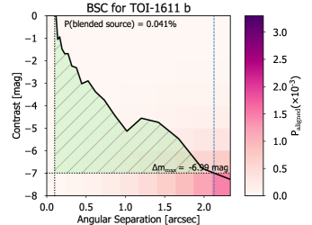
Figure 1: Blended Source Confidence (BSC) curve from the AstraLux SDSSz image (solid black line). The color on each angular separation and contrast bin represents the probability of a chance-aligned source with these properties at the location of the target, based on TRILEGAL model (see Sect. 2.3 within the main text). The maximum contrast of a blended binary capable of mimicking the planet transit depth is shown as a dotted horizontal line. The green-shaded region represents the non-explored regime by the high-spatial resolution image. The BSC corresponds to the integration of $P_{\rm aligned}$ over this shaded region.

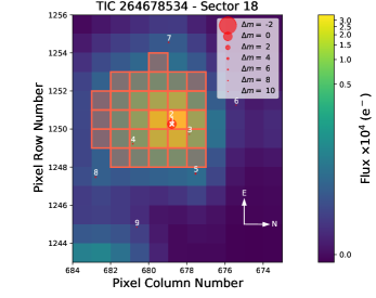
Figure 2: Target Pixel File of TESS for HD207897 corresponding to sector 18, created with tpfplotter (Aller et al. 2020). The red square is related to the SPOC aperture mask and red circles indicate Gaia DR2 magnitude of nearby stars with the size of depending on their brightness. HD207897, number 1, has a Gaia(mag) = 8.1 while the nearest star TIC 264678535, number 2, has a Gaia(mag)=13.8.

By using this sensitivity curve, we additionally estimated the probability of an undetected blended source in our high-spatial resolution image (BSC, see procedure described in Lillo-Box et al. 2014). We use a python implementation of this approach (bsc, by J. Lillo-Box) which uses the TRILEGAL galactic model (v1.6 Girardi et al. 2012) to retrieve a simulated source population of the region around the corresponding target. This simulated population is used to compute the density of stars around the target position (radius $r=1^{\circ}$) and derive the probability of chance-alignment at a given contrast magnitude and separation. In this case, given the AstraLux high-resolution image, we obtain a probability of an undetected blended source of 0.041%. We consider this probability low and the odds that such an undetected source being an appropriate binary capable of mimicking the transit signal to be negligible. In addition, by using tpfplotter code (Aller et al. 2020), we plotted the Target Pixel File from TESS for HD207897 b (see Fig.2). We checked for possible light contamination by considering the nearby stars TIC 264678535 ($T_{mag}=13.3$), TIC 264678538 ($T_{mag}=15.69$) and TIC 264678529 ($T_{mag}=14.39$), all inside the selected apertures analyzed by PDC-SAP. Since the Gaia G band-pass is quite similar to TESS band-pass, we used the Gaia fluxes of these stars and estimated the level of contamination. The total flux due to nearby stars was only $0.8\%$ of HD207897’s flux which is automatically corrected by SPOC. Given the low probability of undetected blended sources from the AstraLux high-resolution image, negligible amount of light contamination due to nearby stars, and similar Keplerian amplitudes derived with different masks (see Sect. 3.3.1), we conclude that the transit and RV variations originate from the main target within the TESS TPF (HD207897), and are of planetary origin.

3 Analysis and Results

3.1 Stellar parameters

To obtain the stellar atmospheric parameters, we first summed the 66 spectra of SOPHIE after correcting from RV variations of the star, barycentric Earth radial velocity, and background correction of calibration lamps (Hobson 2019). It resulted in a high S/N per pixel spectrum of 772 at 550 nm.

The $T_{eff}$ and [Fe/H] were calculated following the procedure described in Santos et al. (2013) and Sousa et al. (2018). It is based on the equivalent width of Fe I and Fe II lines and assumes a balance in excitation and ionization of iron lines in local thermal equilibrium. Abundances of Mg and Si were derived closely following the curve-of-growth analysis methods described in our previous works (Adibekyan et al. 2012, 2015). Abundances of C and O are very difficult to determine for stars cooler than about 5200 K (Delgado Mena et al. 2010; Bertran de Lis et al. 2015). We estimated the abundances of these elements empirically by using a machine learning algorithm (we used the estimator ”RandomForestRegressor”) from the Python Scikit-learn package (Pedregosa et al. 2011). The estimation of C and O was based on the abundance of Mg and Fe (Delgado Mena et al. 2017). Our initial sample was based on the HARPS sample for which abundances of Mg and Fe are available (Adibekyan et al. 2012). Then we derived O abundance for 535 stars and C abundance for 758 stars following the methodology of our previous works (Delgado Mena et al. 2010; Bertran de Lis et al. 2015). These samples were used as training and test datasets. The resulting abundances and other stellar parameters of HD207897 are presented in Table 1.

As an independent Stellar Classification analysis, we used the FIES and TRES data following (SPC; Buchhave et al. 2012, 2014). The FIES analysis uses five spectral orders spanning a wavelength range from 5065 to 5320 Å, while the TRES analysis uses three spectral orders spanning the range from 5060 to 5300 Å. The spectra were compared to a library of synthetic templates, to measure the effective temperature $T_{\rm eff}$, surface gravity $\log g$, projected rotational velocity $v\sin i$, and metallicity [m/H] (a solar mix of metals). We analyzed the spectra individually and calculated a weighted average of each parameter. The results were $T_{\rm eff}=5085\pm 50{\rm K}$, $\log g=4.48\pm 0.10$, $v\sin i<2{\rm kms}^{-1}$, and [m/H]$=-0.23\pm 0.08$ which are in agreement with the other methods.

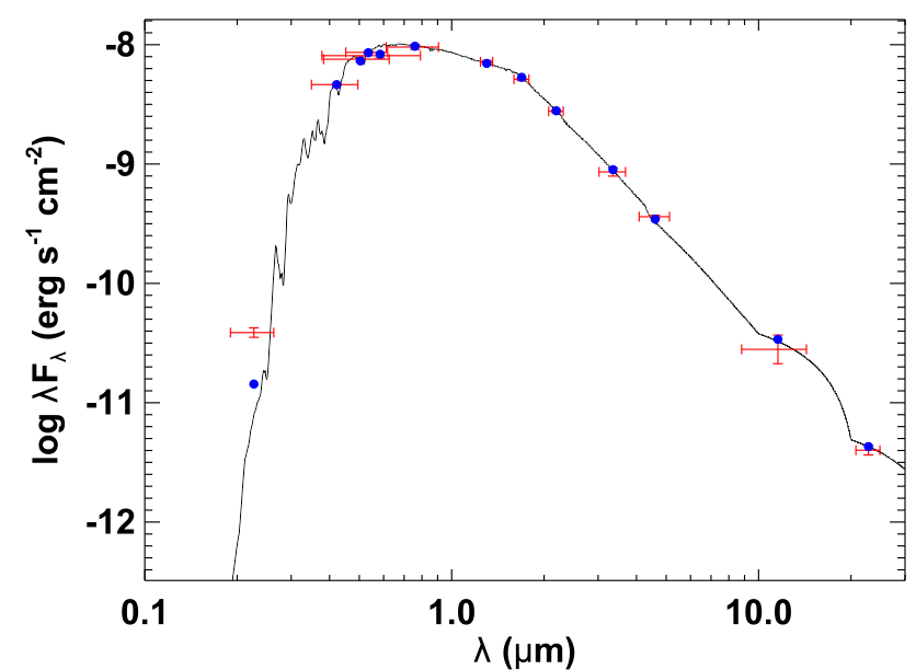
Figure 3: Spectral energy distribution of HD207897. Red symbols represent the observed photometric measurements, where the horizontal bars represent the effective width of the passband. Blue symbols are the model fluxes from the best-fit Kurucz atmosphere model (black).

We also performed an analysis of the broadband spectral energy distribution (SED) of the star together with the Gaia EDR3 parallax (with no systematic offset applied; see, e.g., Stassun & Torres 2021), in order to determine an empirical measurement of the stellar radius, following the procedures described in Stassun & Torres (2016); Stassun et al. (2017a, b). We pulled the $B_{T}V_{T}$ magnitudes from Tycho-2, the $JHK_{S}$ magnitudes from 2MASS, the W1–W4 magnitudes from WISE, the $GG_{\rm BP}G_{\rm RP}$ magnitudes from Gaia, and the NUV magnitude from GALEX. Together, the available photometry spans the full stellar SED over the wavelength range 0.2-22 $\mu$m (see Figure 3).

We performed a fit using Kurucz stellar atmosphere models, with the effective temperature ($T_{\rm eff}$), metallicity ([Fe/H]), and surface gravity ($\log g$) adopted from the spectroscopic analysis. We also fixed the extinction $A_{V}\equiv 0$ based on the star’s proximity (see Table 1). The resulting fit (Figure 3) has a reduced $\chi^{2}$ of 1.1, excluding the GALEX NUV flux which indicates a moderate level of activity. Integrating the (unreddened) model SED gives the bolometric flux at Earth, $F_{\rm bol}=1.401\pm 0.016\times 10^{-8}$ erg s^-1 cm^-2. Taking the $F_{\rm bol}$ and $T_{\rm eff}$ together with the Gaia parallax, gives the stellar radius, $R_{\star}=0.785\pm 0.014$ R_⊙. In addition, we can estimate the stellar mass from the empirical relations of Torres et al. (2010), giving $M_{\star}=0.84\pm 0.05$ M_⊙. Additionally, we cross-checked these values with a different methodology by EXOFASTv2 in Sect 3.4.

Table 1: Stellar properties of HD207897

Other identifiers
	TIC 264678534
	HD 207897
	BD +83 617
	HIP 107038
	Gaia DR2 2300641567596591488
	2MASS J21404490+8420005
Parameter	HD207897	References
	Astrometric properties
Parallax (mas)	$35.3446\pm 0.0468$	$GaiaDR2^{*}$
	$35.3581\pm 0.0159$	$GaiaEDR3$
Distance	28.25 $\pm$ 0.03	Gaia DR2
$\alpha(hms)$	$21:40:44.78$	Gaia DR2
$\delta(dms)$	$+84:20:00.56$	Gaia DR2
	Photometric properties
B-V	$0.86\pm 0.02$	HIP
V(mag)	$8.37\pm 0.0015$	HIP
Gaia(mag)	$8.1304\pm 0.0004$	Gaia DR2
$Gaia_{BP}(mag)$	$8.6051\pm 0.0025$	Gaia DR2
$Gaia_{RP}(mag)$	$7.5402\pm 0.0014$	Gaia DR2
TESS(mag)	$7.58\pm 0.006$	TESS
J(mag)	$6.830\pm 0.023$	2MASS
H(mag)	$6.391\pm 0.034$	2MASS
$K_{s}(mag)$	$6.312\pm 0.026$	2MASS
$W_{1}(mag)$	$6.262\pm 0.088$	WISE
$W_{2}(mag)$	$6.219\pm 0.025$	WISE
$W_{3}(mag)$	$6.275\pm 0.015$	WISE
$W_{4}(mag)$	$6.233\pm 0.045$	WISE
	Spectroscopic properties
Spectral type	K0V	HIP
$\xi_{t}$ $(kms^{-1})$	$0.53\pm 0.10$	Sec 3.1
$\log(R^{\prime}_{HK})$	$-4.83\pm 0.10$	Sec 3.3.2
$v\sin i$ $(kms^{-1})$	$<2$	Sec 3.3.2
$[Fe/H]$ $dex$	$-0.21\pm 0.02$	Sec 3.1
$[C/H]$ $dex$	$-0.23\pm 0.07$	Sec 3.3.2
$[O/H]$ $dex$	$-0.11\pm 0.08$	Sec 3.3.2
$[Mg/H]$ $dex$	$-0.17\pm 0.06$	Sec 3.3.2
$[Si/H]$ $dex$	$-0.19\pm 0.05$	Sec 3.3.2
	Bulk properties
Mass ($M_{sun}$)	$0.80^{+0.036}_{-0.030}$	Sec 3.4
	$0.84\pm 0.05$	Sec 3.1
Radius($R_{sun}$)	$0.779^{0.019}_{-0.018}$	Sec 3.4
	$0.785\pm 0.014$	Sec 3.1
$\log{g}(cgs)$	$4.559^{+0.026}_{-0.025}$	Sec 3.4
$L_{s}(L_{sun})$	$0.360^{+0.019}_{-0.014}$	Sec 3.4
$T_{eff}(K)$	$5070^{+60}_{-57}$	Sec 3.4
$P_{rot}(days)$	$37\pm 7$	Sec 3.3.2

3.2 Photometry data analysis

The photometry was extracted with the Pre-search Data Conditioned Simple Aperture Photometry (PDC-SAP) pipeline (Stumpe et al. 2012; Smith et al. 2012; Stumpe et al. 2014) provided by the TESS team. We removed nans, flagged low-quality data, and $5\sigma$ outliers. We then normalized and detrended the light curve with a spline robust iterative sigma-clipping method (Schoenberg 1946) using the Wotan package (Hippke et al. 2019) . This method detrends the light curve by fitting the spline through minimizing the sum of squared residuals along with iteratively sigma-clipping. This step is one of the most important steps in the photometric analysis as it reduces the number of false-positive signals by removing instrumental and stellar noise. On the other hand, with such detrending algorithms, there is always a risk of changing the transit depth or even fully removing shallow transits. For this reason, we tested different values of knots and chose the value of 0.7, which was the maximum value that seemed enough for removing the light curve variabilities. The resulting light curve is shown in Figure 4 with the transit events marked with red triangles.

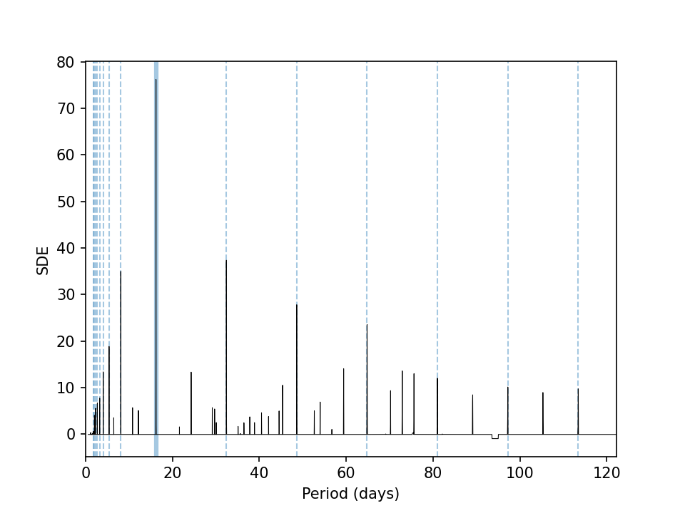
Figure 11: TLS periodogram for the TESS light curve of HD207897 b. The blue line shows the highest peak at 16.20 d with SDE=76.2. The dashed blue lines indicate the aliases of this period.

To look for any periodic signals in the data, we used the transit-least-squares (TLS) algorithm (Hippke & Heller 2019), a method to investigate planetary transits taking into account the stellar limb-darkening (Mandel & Agol 2002) and also the effects of planetary ingress and egress. This method is publicly available and has been optimized for Signal Detection Efficiency (SDE) of small planets. We searched for periodic signals in the range 0.6 to 122 d and sampled 28607 periods within that range. The result showed a prominent periodic signal occurring every 16.20 d with a S/N of 43, giving a SDE of 76.2 and a false alarm probability (FAP) below 0.01 % (see Fig 11). After masking the signal at 16.20 d, we ran the TLS again and did not see any periodic signals. A search for a long-period beyond 122 d did not show any significant signals either.

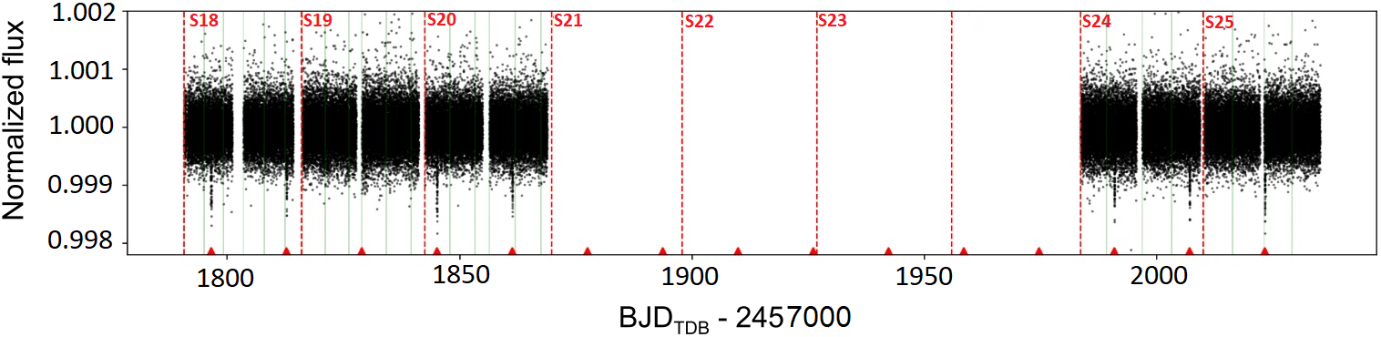
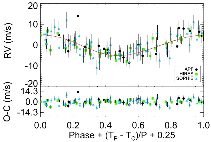
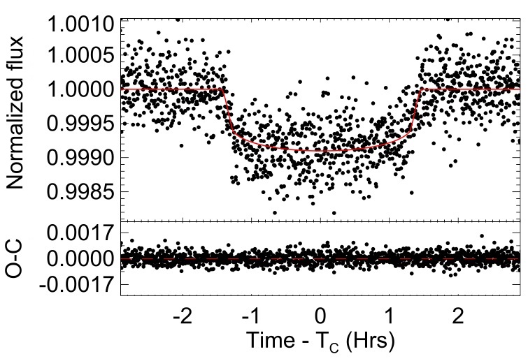
Figure 4: TESS light curves and EXOFASTv2 best fit models on RVs and phometric data. Top panel: The Full PDC-SAP (2-minute) TESS light curve after detrending, taken from sectors 18, 19, 20, 25 and 26. The red triangles indicate the transit events, and the green vertical lines indicate the momentum dumps of spacecraft which occurs every 2.5 days. None of the transit events fall during momentum dumps. Bottom left: Phase-folded SOPHIE, APF, and HIRES RVs of HD207897 b at the period of 16.20 d. Bottom right: TESS Phase-folded light curve.

3.3 Radial velocity data analysis

3.3.1 RVs data reduction on SOPHIE

The SOPHIE data were reduced with the SOPHIE Data Reduction pipeline (DRS, Bouchy et al. 2009b), which extracts the RV by cross-correlating spectrum with a binary mask and then doing a Gaussian fit of the cross-correlation function (CCF) (Pepe et al. 2002). We tested different masks, including G2, K0, and K5. Since they showed similar Keplerian amplitude variations, it is unlikely that these variations are produced by blend scenarios composed of stars of different spectral types (Bouchy et al. 2008). We finally adopted the RV data derived with the K5 mask as it presented a smaller RV dispersion.

We subsequently excluded 6 RV points that did not reach the required quality: 3 points with a lower signal-to-noise than required $S/N_{550}>50$, 2 points with moonlight pollution, and 1 point both being an outlier and resulting from an observation performed with no simultaneous calibration. We corrected the remaining points for the charge transfer inefficiency (CTI) effect (Santerne et al. 2012). This correction ranged from 1.4 to 6 m s^-1 with a mean RV correction of 2.1 m s^-1. Afterward, we removed the nightly drift of the telescope measured from the simultaneous Th-Ar or FP reference spectra. This correction also falls within the 0.1 to 9 m s^-1range, with a mean RV of 2.1 m s^-1.

The next step was removing a long-term drift of the zero point due to the instrumental effect identified in SOPHIE RV data (Courcol et al. 2015; Hobson et al. 2018). To track this offset, so-called ’constant’ stars have been monitored each night. We combined these observations to build a time series of the RV master constant (see Courcol et al. (2015) for more details on the method). We then estimated long-term zero point drift as a function of time for each night of observation and subtracted it from the HD207897 RV data. This correction is in the 0.2 to 6 m s^-1 range with a mean value of 3.3 m s^-1. Since we saw the effects of the long-term drift of the zero points on the bisector span of constant stars, we applied the same processes to the bisector of HD207897 as well. The correction for bisector was between 4 to 11 m s^-1 with a mean value of 2 m s^-1. Once these corrections were applied, the HD207897 RVs reduced from an original RMS of 6.2 m s^-1 to a final RMS of 4.9 m s^-1.

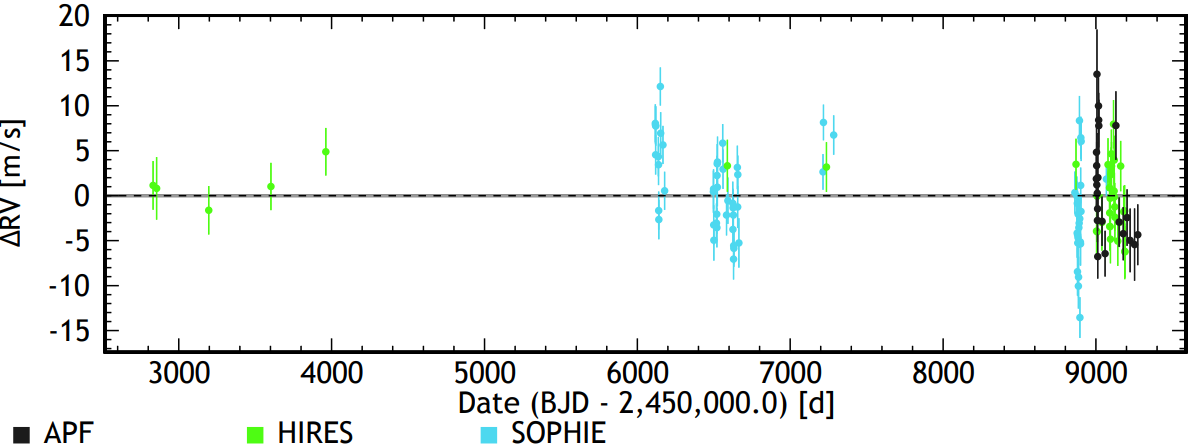
Figure 5: Radial velocities of HD207897 from SOPHIE, APF and HIRES, before linear trend correction.

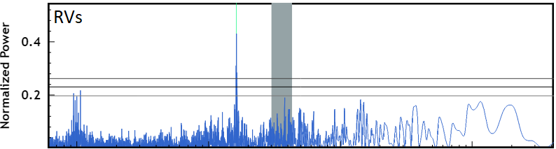
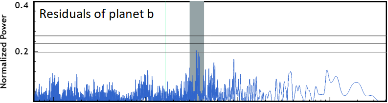
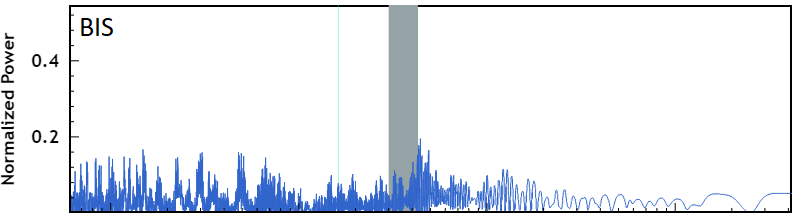
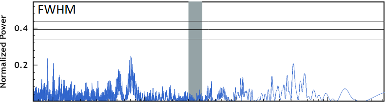
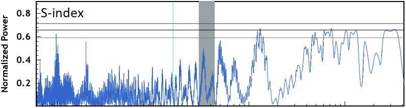
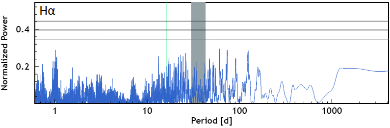
Figure 6: Normalized periodograms of RVs and activity indexes for HD207897. From top to bottom panel: RVs, residual of RVs after Keplerian fit on 16.20 d, Residuals of fit on planet and stellar rotation signal, CRX, bisector, FWHM, and $H\alpha$ index. The cyan vertical line marks the position of the highest peak at RVs periodogram at 16.20 d and shows no corresponding peak in the stellar activity periodograms. Horizontal lines indicate 0.1, 1, 10 $\%$ FAP level, from top to bottom, respectively. Also, the grey vertical strip is highlighting the position of the estimated rotational period of star in Sect. 3.3.2

3.3.2 Stellar rotation and activity

To investigate the activity of the star, we used several indicators such as bisector span, CCF FWHM, Chromatic RV index (CRX), $H\alpha$, and $\log(R^{\prime}_{HK})$ from SOPHIE spectra as well as S-index from the HIRES spectra.

We obtained the bisector span and CCF FWHM from the SOPHIE data reduction system. The CRX is extracted using SERVAL (Zechmeister et al. 2018) code. To compute the $H\alpha$ index, which measures the flux in the $H\alpha$ line, we followed the definitions of Boisse et al. (2011). To do so, we also applied background correction to the data as appropriate for the two different calibration lamps (for further details, see Hobson 2019).

We derived the S-index from HIRES spectra following Baliunas et al. (1995) and Paulson et al. (2002). We also computed the $\log(R^{\prime}_{HK})$ index on SOPHIE spectra, following the method of Noyes et al. (1984), but the S/N is low in all first (bluest) orders, where Ca H&K lines are located, with one exception in 2020 (S/N =33). We decided to sum the bluest order of spectra with S/N ¿ 20 to reach to better S/N ratios and then calculate $\log(R^{\prime}_{HK})$. We first did so for the 2012-2015 spectra, of which 22 had a S/N ¿ 20, giving a value of $\log(R^{\prime}_{HK})=-4.83\pm 0.10$. Only one 2020 spectrum presents a S/N ¿ 20, so no summation was possible. This spectrum yields a value of $\log(R^{\prime}_{HK})=-4.78\pm 0.10$, indicating that the star may have a similar level of activity as during the 2012-2015 period. Our value of $\log(R^{\prime}_{HK})$ for 2012-2015 is consistent with $\log(R^{\prime}_{HK})=-4.86$ reported by Brewer et al. (2016). This value indicates a modest activity level of HD207897.

To check our $\log(R^{\prime}_{HK})$ value, we used the star’s GALEX NUV flux excess (Fig. 3). The observed NUV excess implies a chromospheric activity of $\log R^{\prime}_{rmHK}=-4.82\pm 0.05$ via the empirical relations of Findeisen et al. (2011), consistent with the value obtained spectroscopically. Moreover, the NUV estimated activity implies an age of $\tau_{\star}=4.4\pm 0.9$ Gyr via the empirical relations of Mamajek & Hillenbrand (2008).

We estimated a stellar rotation period of $37\pm 7$ d with the method proposed in Noyes et al. (1984), which is in good agreement with an estimated period of $36^{+5}_{-4}$ d following Mamajek & Hillenbrand (2008). These estimates are consistent with the value of 38 days from Isaacson & Fischer (2010).

We sought to constrain the $P_{rot}$ of the star with RVs and activity indicators. We subtracted a linear drift in the CCF FWHM, CRX, and RVs time series, and a cubic drift in the S-index. Also, an offset term is fitted on $H\alpha$ data between the two different calibration lamps background correction (before and after BJD= 57284.4185). Then, we computed the periodogram of RVs, the RV-residuals of keplerian models, and activity indicators (Fig 6). The RV-residuals of planet b show two peaks at 35.9 and 37.6 days near to 10 % FAP.

We ran an $\ell_{1}$ periodogram on the RVs (see Fig. 7) for comparison. This one is obtained with the same procedure as in Hara et al. (2020): we considered alternative noise models characterised by an autocovariance function that is a sum of white, correlated, and quasi-periodic components with different amplitudes and time scales and ranked them with cross-validation. The correlated component is a Gaussian kernel characterised by its time-scale and amplitude, the quasi-periodic component is a Gaussian Kernel as in Haywood et al. (2014) characterised by its decay time-scale, period, and amplitude. The amplitudes of the white, correlated, and quasi-periodic terms are taken on a grid (0 to 3 m/s with a 0.5 m/s step), the time-scales 0,3,6 days for the correlated term and 30, 60, 90 days for the quasi-periodic term and 37.6 days for the period of the quasi-periodic component. We also included in the base model one offset per instrument. Figure 7 corresponds to the highest ranked noise model. We found a significant signal at the planet period (FAP of $2\cdot 10^{-9}$) and found a signal at 37.6 d with a FAP of 0.5. The signal at 37.6 d very likely corresponds to a stellar signal.

While the periodogram of CCF FWHM and $H\alpha$ activity indicators do not exhibit any significant signals, CRX shows a peak near to 10 % FAP at 36.5. The S-index periodogram shows several peaks at the long periods, however, no correlation (R= 0.16) is found between the S-index and HIRES RVs. We note that given the relatively small value of $v\sin i$ ($2\pm 1$ km s^-1), we could not see any correlations between the RVs and its residuals and bisector.

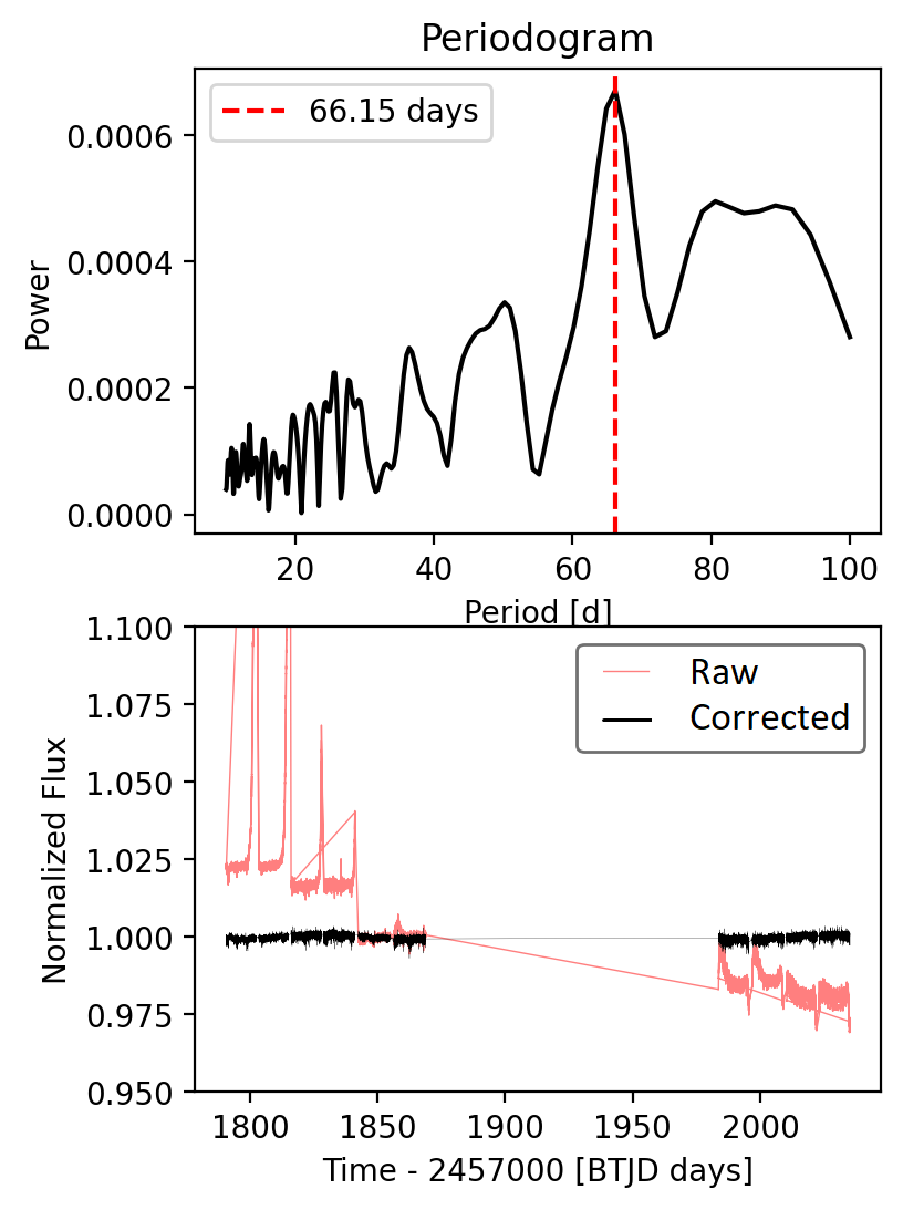
Figure 12: Top: Systematics-Insensitive Periodogram (SIP) for HD207897 b. Bottom: raw SAP TESS light curves in red and detrended data against instrument systematics by SIP in black. The SIP periodogram does not exhibit any significant signal for HD207897 b, since the highest peak in this periodogram has a power of only 0.0006 at 66.6 d.

We searched the SAP and PDC-SAP light curves for a signal of the rational period of the star in the photometry. For this, we applied the Systematics-insensitive Periodogram (SIP) method (Angus et al. 2016; Hedges et al. 2020) for SAP, and Gaussian process (GP) model on PDC-SAP light curves. The SIP method detrends SAP light curve (see Fig. 12 bottom) from TESS instrument systematics, along with calculating Lomb–Scargle periodogram and without requiring pre-detrending light curves as other methods (e.g. AutoCorrelation Function (ACF) by McQuillan et al. 2013). This method was initially used for the Kepler mission and has recently been successfully applied for TESS data such as TOI-1259A (Martin et al. 2021) and TOI-700 (Hedges et al. 2020). The SIP periodogram (see Fig. 12 top) does not exhibit any significant signal for HD207897 b. Also applying a GP model on PDC-SAP light curves did not display any convincing signal either.

To examine further the origin of the 37.6 d signal, following Hara et al. (2021), we check for the phase and amplitude consistency of the 37.6 days signal in the SOPHIE RVs. We use the statistic defined in Eq. 14 of Hara et al. (2021). We fit an offset and a linear trend as well as a sinusoidal model for the 16.2-day planet. Adopting the value of the RV jitter of 3.16 m s^-1, we find that the hypothesis that the phase and amplitude of the 37.6-day signal is constant is rejected at $2\sigma$, which further supports the hypothesis that this signal is due to activity.

Given the estimated stellar rotational period value and the signal at the CRX activity indicator, it is likely the signals at 35.9 and 37.6 days are due to the stellar rotation period. We take into account these peaks in our joint model analysis with EXOFASTv2 in Sect 3.4.

3.3.3 Radial velocities results

The combined RV data of HD207897 are plotted in Fig. 5 after fitting a zero-points offset for each RV dataset (see table 3). We removed a linear trend of $-0.28\pm 0.11$ m s^-1 yr^-1 from RVs. We note that no notable differences were found in our results by including/excluding this linear drift. However, since we saw a clear linear drift in the activity indicators such as the CCF FWHM and CRX we decided to keep the drift.

We investigated the footprints of the planet in RVs by searching for periodic signals. To do so we used the Data and Analysis Center for Exoplanets (DACE, Delisle et al. 2016) web platform and computed periodograms for the RVs (Fig: 6).

The RVs periodogram displays a clear peak at 16.20 d with a value below 0.1 % false alarm probability (Baluev 2008). Moreover, there is no corresponding peak in the periodogram of activity indicators, which shows that this periodic signal is likely due to a planet and not due to stellar activity, Figure 6.

As it is shown in Figure 7, the $\ell_{1}$ periodogram confirms that the most prominent signal appears at 16.20 days with FAP of $2\cdot 10^{-9}$. The value of the second-highest peak at 37.7 days is in agreement with the estimated rotational period of the star (see Section 3.3.2).

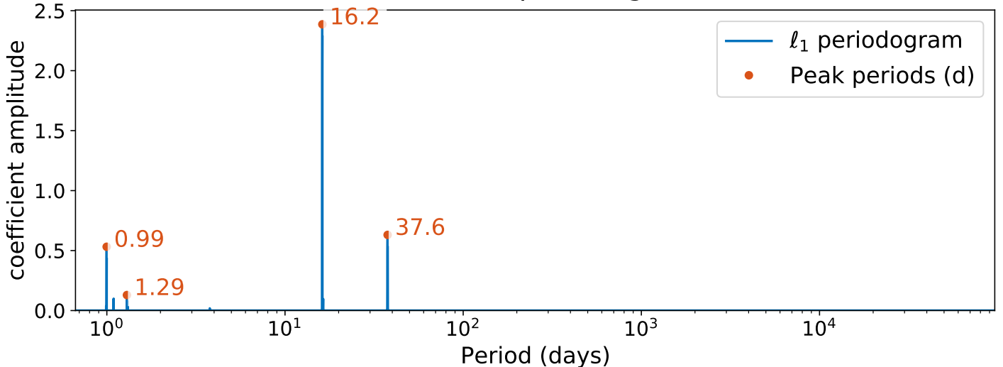
Figure 7: $\ell_{1}$ periodogram of SOPHIE RVs for HD207897 b, following Hara et al. (2017). The main peaks of the periodogram are indicated

with orange circles.

3.4 Joint modeling of RV and photometry

To explore all the parameters of the system, including both the host star and the planet, we modeled simultaneously and self-consistently the photometric observations of the star from five sectors of TESS, and the RV observations from SOPHIE, HIRES, and APF using the Fast Exoplanetary fitting package (EXOFASTv2 , Eastman et al. 2013; Eastman 2017; Eastman et al. 2019). This global modeling software uses a differential evolution Markov Chain coupled with a Metropolis-Hastings Monte Carlo sampler that uses error scaling for exploring the system parameters.

EXOFASTv2 fits a total of 33 free parameters for the HD207897 system, which can be divided into the following categories:

• twelve parameters related to the planet and activity period: the mid-transit time $T_{C}$, planet orbital period $P$, the planet-to-star radius ratio $R_{p}/R_{star}$ (only for planet), the orbital inclination $i$ (only for planet), the RV semi-amplitude $K$, and two more free parameters related to eccentricity $e$.

• Two parameters for each RV instrument: instrumental offset and jitters. One free parameter is also fitted for drift on RVs.

• Two limb darkening coefficients for TESS photometric bands pass, along with baseline flux and variance are fitted for the transit light curve.

• Eleven stellar parameters: Stellar mass $M_{*}$, Stellar radius $R_{*}$ and effective temperature $T_{eff}$ by the MIST model, Stellar radius $R_{*,SED}$ and effective temperature $T_{eff,SED}$ by the SED model, observed metallicity $[Fe/H]$, theoretical metallicity at the star’s birth $[Fe/H]_{0}$ by MIST model, Age , equivalent evolutionary point $EPP$, V-band extinction $A_{v}$ and distance $d$.

Before running EXOFASTv2, we set a Gaussian prior on $T_{eff}$ and [Fe/H] from our spectral analysis results, presented in Sect 3.1. We also imposed a prior on the Gaia DR2 parallax after applying the offset correction as described in Lindegren et al. (2018). Broadband photometry presented in Table 1 is also included. We enforced an upper limit for the V-band extinction ($A_{v}$) from Schlegel et al. (1998) and Schlafly & Finkbeiner (2011). The broadband photometry, the Gaia parallax, and the $A_{v}$ allowed us to model the stellar spectral energy distribution, a key to constrain the stellar radius. Indeed, EXOFASTv2 interpolates a pre-compiled 4d grid of bolometric corrections (logg, $T_{eff}$, [Fe/H], reddening) to arrive at the broadband photometry flux directly. We did not set the limb darkening to let EXOFASTv2 constrain the best parameters of a quadratic limb darkening through the Claret (2017) tables for TESS bands and the stellar atmosphere’s parameters ($T_{eff}$, [Fe/H] index and log $g_{*}$). We used the Mesa Isochrones and Stellar Tracks evolutionary model (MIST, Dotter 2016; Choi et al. 2016) to derive the full stellar parameters by combining our data. We also allowed the fitting of a linear slope on the original RVs as part of our joint analysis.

EXOFASTv2 considers the chains to be well-mixed when the Gelman-Rubin statistic (Gelman et al. 2004, 1992; Ford 2006) decreases below 1.01. The Gelman-Rubin statistic describes how similar the chains are; a value under 1.01 shows the chains are well-mixed. The list of our priors and final median values of the posterior distributions, and their 1 $\sigma$ confidence intervals of full system parameters are reported in table 3.

As we showed in Sect 3.3.2, HD207897 has a moderate stellar activity and the signals at 35.9 and 37.6 d are likely to be due to the stellar rotation periods. Since these signals affect slightly the mass estimate of the planet, we considered them as an additional keplerian fit in our global analysis. A more ideal solution to take activity into account is de-trending the RVs using activity indicators (e.g. S-index, FWHM), but currently, it is not possible with EXOFASTv2. Furthermore, to de-trend we did not have the same activity indicators for all RVs. As an independent analysis, we used only SOPHIE data and trained GP against CRX, the results were completely in agreement with EXOFASTv2 global modeling. When using two Keplerian models in EXOFASTv2, we did not fix the period and let EXOFASTv2 find the best activity period between the 35.9 and 37.6 d signals. After EXOFASTv2 converged, we saw a bimodality in the posterior distribution for the stellar activity periods (see Fig. 8, top), so we present the final median posterior distribution values of both the most probable solutions in Table 3. We also report their calculated probabilities based on the area of the posterior distributions. The probability of the most likely values is 54% and that of the less likely values is 46%.

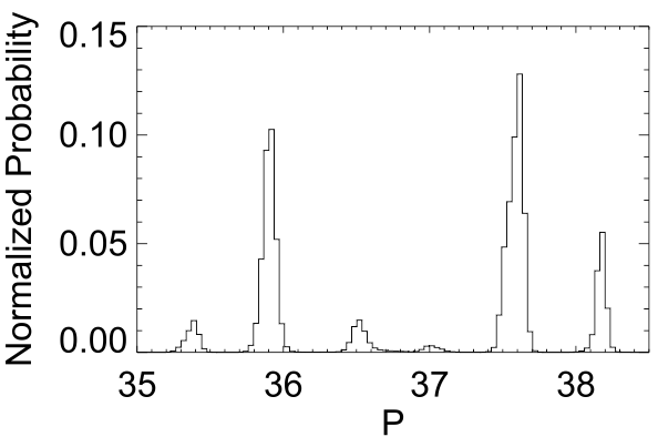
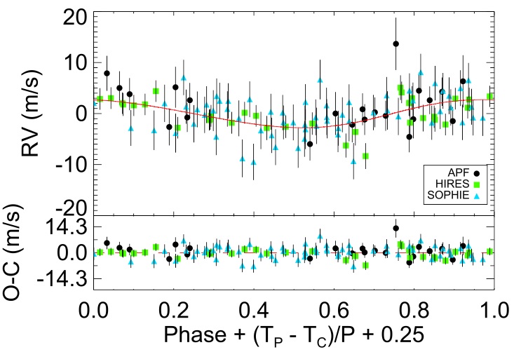
Figure 8: Top: Bimodality in the posterior distribution for the stellar activity periods. Bottom: Solution of the two-Keplerian model on the activity signal at 37.6 d with the initial period at 16.2 d.

HD207897 is a main-sequence K0 dwarf star. We found that its most likely values for: mass is $0.800^{+0.036}_{-0.030}$ $M_{\sun}$, radius is $0.779^{+0.019}_{-0.018}$ R_☉ and T_eff is $5070^{+60}_{-57}$ K. These values are in good agreement with the result of our stellar analysis in Sect. 3.1 and also, the stellar parameters from Gaia Data Release 2, such as T_eff= $5052^{+114}_{-78}$ K and radius of $0.79^{+0.80}_{-0.75}$ R_☉ (Brown et al. 2018)

We also show that the planet has a period of 16.20 d, a radius of $2.5\pm 0.08$ R_E and a mass of either $14.4\pm 1.6$ M_E or $15.9\pm 1.6$ M_E with nearly equal probability. These two solutions correspond to two possibilities for the stellar activity period. Hence, the density is either $5.1\pm 0.7$ g cm^-3 or $5.5^{+0.8}_{-0.7}$ g cm^-3. Both values are in agreement with each other inside their error bars.

The keplerian solution and transit model for HD207897 b on the most likely values are shown in Fig. 4 (bottom). Also, the keplerian model on the most likely activity period on 37.6 d is illustrated in Fig. 8.

4 Internal structure

In order to characterise the internal structure of HD207897 b, we have performed a Markov chain Monte Carlo (MCMC) Bayesian analysis (Dorn et al. 2015) using the interior composition model introduced in Brugger et al. (2017), Mousis et al. (2020) and Acuña et al. (2021), which comprises three layers: a Fe-rich core, a silicate rich mantle and a water layer. With an input equilibrium temperature of 637 K, assuming an albedo of zero, the irradiance HD207897 b received is enough to present vapour and supercritical phases if water is found on its surface. Therefore we coupled an atmosphere-interior model that calculates the surface conditions and the contribution of the atmosphere to the total radius.

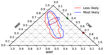
Figure 9: 2D, 1$\sigma$ confidence regions of HD207897 b for the mass estimation with activity period on 37.6 d (blue) and with activity period on 35.9 d (red). Solid lines indicate the confidence intervals of scenario 1, while dashed lines correspond to scenario 2, where the stellar abundances are also included as input data in the MCMC interior structure analysis. The mantle mass fraction (MMF) is defined as MMF = 1 - CMF - WMF. The green dot and brown square indicate the position of Earth and Mercury in the ternary diagram, respectively.

We considered two scenarios to obtain the interior structure of HD207897 b: scenario 1, where only the mass and radius of the planet are considered as inputs to the MCMC analysis (shown in Table 3); and scenario 2, where the planetary mass and radius, and the stellar Fe/Si and Mg/Si mole ratios (see Table 1) are the input data. To compute the Fe/Si and Mg/Si mole ratios with the stellar abundances, we follow the approach depicted in Brugger et al. (2017) and Sotin et al. (2007), and obtain Fe/Si = 0.74$\pm$0.09 and Mg/Si = 1.11$\pm$0.20. The outputs of the MCMC analysis are the posterior distributions functions (PDF) of the core mass fraction (CMF), the water mass fraction (WMF) and the atmospheric parameters, which are the temperature at 300 bar, the planetary albedo and the atmospheric thickness from transit pressure to 300 bar. We assume a water-rich atmosphere. Table 2 shows the 1D, 1$\sigma$ confidence intervals of the MCMC output parameters.

In the most general case (scenario 1), up to 31% of HD207897 b’s mass can be in the form of a hydrosphere reaching supercritical or superionic phases at its base (Mazevet et al. 2019) with the most likely value of the mass. This value increases slightly with the less likely value although both cases are consistent with a water-rich planet with a water mass fraction of 20 to 30 %. The 1$\sigma$ confidence interval limits the maximum CMF to 0.50 (see Figure 9). In addition, a Fe-depleted planet (CMF = 0) is possible, although unlikely. Assuming a pure silicate interior, the WMF is found to be 2.2 x $10^{-5}$ in HD207897 b, which corresponds to a pressure at the base of the hydrosphere of approximately 300 bar.

If we take into account the stellar abundances to constrain the planetary Fe/Si and Mg/Si mole ratios, the CMF is calculated as 0.21, a value lower than the Earth’s CMF (0.32). In this scenario, the WMF would be below 0.16, implying that HD207897 b can be considered a water-rich planet. If the temperature and pressure of the hydrosphere are high enough to sustain a supercritical regime, then the atmosphere is extended and constitutes approximately 20% of the planet’s total radius.

5 Discussion and Summary

In this paper, we detected and characterized a sub-Neptune orbiting around HD207897, with a period of $16.202161\pm 0.000083$ d, using TESS photometry data along with SOPHIE, HIRES, and APF RVs observations. We found the planet has a mass of $14.4\pm 1.6$ M_E with probability of 56 % (or $15.9\pm 1.6$ M_E with probability of 46 % based on bimodal results of stellar activity

	Activity on 37.6 d		Activity on 35.9 d
Parameter	Scenario 1	Scenario 2	Scenario 1	Scenario 2
Core mass fraction, CMF	0.26$\pm$0.18	0.19$\pm$0.03	0.23$\pm$0.18	0.19$\pm$0.03
Water mass fraction, WMF	0.22$\pm$0.09	0.19$\pm$0.07	0.25$\pm$0.10	0.21$\pm$0.07
Temperature at 300 bar, T300 [K]	2715$\pm$22		2742$\pm$24	2737$\pm$24
Thickness at 300 bar, z300 [km]	234$\pm$22		265$\pm$26	257$\pm$25
Albedo, ap	0.26$\pm$0.01
Core+Mantle radius, [Rp units]	0.72$\pm$0.08	0.75$\pm 0.05$	0.70$\pm$0.08	0.74$\pm$0.05

Table 2: 1$\sigma$ confidence intervals of the interior and atmosphere MCMC output parameters in the two different compositional scenarios (see text).

period) and a radius of $2.5\pm 0.08$ R_E, which translates into a high density of $5.1\pm 0.7$ g cm^-3 (or $5.5^{+0.8}_{-0.7}$ g cm^-3). We used the same mass and radii bounds as Otegi et al. (2020) on NASA Exoplanet Data Archive (December 5th, 2020) and plotted in Fig 10 all the sub-Neptune sized planets (2 ¡ R/R_E ¡ 4) with semi-major axis and luminosity determined. As shown in this plot, HD207897 b joins the group of dense sub-Neptunes such as HD 119130 b ($\rho_{P}=7.4^{+1.6}_{-1.5}$ g cm^-3; Luque et al. 2018), GJ143 b ($\rho_{P}=7^{+1.6}_{-1.3}$ g cm^-3; Dragomir et al. 2019), Kepler-10 c ( $\rho_{P}=7.1\pm 1$ g cm^-3; Dumusque et al. 2014), TOI-849 b ($\rho_{P}=5.2^{+0.7}_{-0.8}$ g cm^-3; Armstrong et al. 2020), Kepler-538 b ($\rho_{P}=5.4\pm 1.3$ g cm^-3; Mayo et al. 2019), Kepler-411 b ($\rho_{P}=9.9\pm 1.3$ g cm^-3; Sun et al. 2019), K2-110 b ($\rho_{P}=5.2\pm 1.2$ g cm^-3; Osborn et al. 2017), and K2-263 b ($\rho_{P}=5.7^{+1.6}_{-1.4}$ g cm^-3; Mortier et al. 2018). These planets are relatively close to their host stars and may have a similar formation history.

How can HD207897 b and other similar planets with such a high density exist at a close distance from their host star? One possibility could be that the planet has lost most of its volatile elements by evaporation, but for the case of HD207897 b with an orbital period of 16.20 d and receiving an incident flux of F=26.3 F_E it is not a satisfactory answer. Indeed, even if we consider an extreme evaporation process (Lecavelier Des Étangs 2007), the mass-loss of the planet would be just 0.1 M_E during the entire lifetime of the star, which cannot account for its high density. HD207897 b is unlikely to have formed in situ. According to Schlichting (2014) the maximum isolation mass that can form at a distance of a = 0.12 AU is only $\sim$ 0.06 M_E, assuming the minimum mass solar nebula (MMSN); a disk surface density $\sim$ 41 times larger than the solar nebula would be required to form a planet as massive as HD207897 b at this distance. Two possible scenarios can however be considered, both consistent with the MMSN: either the material from the outer region migrated and formed the planet HD207897 b (e.g. Chatterjee & Tan 2013) or the formation of HD207897 b occurred far out of the disc and the planet subsequently migrated to its current location (e.g. McNeil & Nelson 2010; Kley & Nelson 2012). The second scenario could have been triggered by another planet in this system. The hint of long-term trend on RVs allows for the presence of another planet. The high occurrence rate of long-period giant planets (mass ¿ 0.3 M_J) in the systems harboring small planets (planets with mass/radius between Earth and Neptune) (Zhu & Wu 2018; Schlecker et al. 2020) can also support such a scenario. In the case of HD 119130 b, Luque et al. (2018) suggested a migration scenario triggered by other planets to explain the linear drift in their RV data. However, more photometry and radial velocity observations are still needed to understand the HD207897 planetary system.

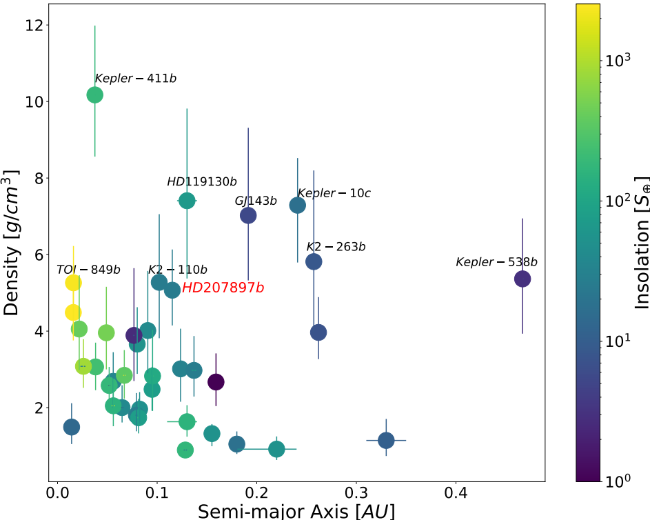
Figure 10: The density-semi major axis diagram for HD207897 b and other sub-Neptune sized planets (2 ¡ R_E ¡ 4) with known semi-major axis, luminosity and accurate mass and radius (Otegi et al. 2020). Dots are colored with planet insolation in Earth unit $(S_{p}/S_{\bigoplus}=(L_{*}/L_{\sun})\times(AU/a_{p})^{2})$. The mentioned planet has a density of above 5 g cm^-3.

Further, the brightness (K= 6.3 mag) of HD207897, its relatively small stellar radius, and its quite nearby distance (28 pc) would make HD207897 b a good target for atmospheric characterization. Similarly, such a close distance and brightness for a transiting planet host, make HD207897 b an excellent target for studying the architecture of the system through ground-based observations. For example, measuring the host star spin-orbit alignment (obliquity) using the Rossiter-McLaughlin (RM, Rossiter 1924; McLaughlin 1924) anomaly can provide us with important information about planetary migration and evolution.

Table 3: Median values and 68% confidence interval for HD207897 b and its host star. Gaussian priors are presented by $\mathcal{N}(a,b)$ where a and b are mean and width value, respectively. Likewise, uniform prior is donated by $\mathcal{U}(c,d)$ and c and d are presenting bounds on the parameter. The two solutions correspond to two possibilities for the stellar activity period. Highlighted parameters are presenting more than 0.5 $\sigma$ difference between the two solutions. See Table 3 in Eastman et al. (2019) for a detailed description of all parameters.

Parameter	Units	Model priors	Activity on 35.9 d (Prob. = 46%)	Activity on 37.6 d (Prob. = 54%)
Stellar Parameters:
$M_{*}$	Mass (M☉)	-	$0.801^{+0.036}_{-0.031}$	$0.800^{+0.036}_{-0.030}$
$R_{*}$	Radius (R☉)	-	$0.779^{+0.019}_{-0.018}$	$0.779^{+0.019}_{-0.018}$
$R_{*,SED}$	Radius1 (R☉)	-	$0.7691^{+0.011}_{-0.0098}$	$0.7692^{+0.011}_{-0.0100}$
$L_{*}$	Luminosity (l☉)	-	$0.360^{+0.019}_{-0.014}$	$0.360^{+0.019}_{-0.014}$
$F_{Bol}$	Bolometric Flux (cgs)	-	$0.00000001440^{+0.00000000076}_{-0.00000000056}$	$0.00000001439^{+0.00000000077}_{-0.00000000055}$
$\rho_{*}$	Density (cgs)	-	$2.39^{+0.19}_{-0.18}$	$2.39^{+0.19}_{-0.18}$
$\log{g}$	Surface gravity (cgs)	-	$4.558^{+0.027}_{-0.025}$	$4.559^{+0.026}_{-0.025}$
$T_{\rm eff}$	Effective Temperature (K)	$\mathcal{N}$[5012,80]	$5071^{+59}_{-57}$	$5070^{+60}_{-57}$
$T_{\rm eff,SED}$	Effective Temperature1 (K)	-	$5096^{+78}_{-54}$	$5096^{+78}_{-54}$
$[{\rm Fe/H}]$	Metallicity (dex)	$\mathcal{N}[-0.21,0.08]$	$-0.040^{+0.037}_{-0.040}$	$-0.042^{+0.038}_{-0.041}$
$[{\rm Fe/H}]_{0}$	Initial Metallicity2	-	$-0.028^{+0.050}_{-0.052}$	$-0.030^{+0.050}_{-0.053}$
$Age$	Age (Gyr)	-	$7.1^{+4.5}_{-4.4}$	$7.1\pm 4.5$
$EEP$	Equal Evolutionary Phase3	-	$343^{+17}_{-26}$	$343^{+17}_{-27}$
$A_{V}$	V-band extinction (mag)	$\mathcal{U}$[0,0.3534]	$0.074^{+0.081}_{-0.052}$	$0.074^{+0.081}_{-0.052}$
$\sigma_{SED}$	SED photometry error scaling	-	$2.10^{+0.77}_{-0.47}$	$2.10^{+0.77}_{-0.48}$
$\varpi$	Parallax (mas)	$\mathcal{N}[35.345,0.047]$	$35.345^{+0.048}_{-0.047}$	$35.345\pm 0.047$
$d$	Distance (pc)	-	$28.292\pm 0.038$	$28.293\pm 0.038$
$\dot{\gamma}$	RV slope4 (m/s/day)	-	$-0.00078\pm 0.00030$	$-0.00077^{+0.00027}_{-0.00028}$
Planetary Parameters:
$P$	Period (days)	-	$16.202157\pm 0.000085$	$16.202159^{+0.000085}_{-0.000083}$
$R_{P}$	Radius ($\,R_{\rm E}$)	-	$2.505^{+0.081}_{-0.077}$	$2.501^{+0.082}_{-0.078}$
$M_{P}$	Mass ($\,M_{\rm E}$)	-	15.9$\pm 1.6$	14.4$\pm 1.6$
$T_{C}$	Time of conjunction5 ($\rm{BJD_{TDB}}$)	-	$2458926.10942^{+0.00047}_{-0.00049}$	$2458926.10942^{+0.00047}_{-0.00048}$
$T_{T}$	Time of minimum projected separation6 ($\rm{BJD_{TDB}}$)	-	$2458926.10944^{+0.00047}_{-0.00049}$	$2458926.10943^{+0.00047}_{-0.00048}$
$T_{0}$	Optimal conjunction Time7 ($\rm{BJD_{TDB}}$)	-	$2458926.10942^{+0.00047}_{-0.00049}$	$2458926.10942^{+0.00047}_{-0.00048}$
$a$	Semi-major axis (AU)	-	$0.1164^{+0.0017}_{-0.0015}$	$0.1163^{+0.0017}_{-0.0015}$
$i$	Inclination (Degrees)	-	$88.755^{+0.067}_{-0.066}$	$88.757\pm 0.067$
$e$	Eccentricity	-	$0.047^{+0.053}_{-0.033}$	$0.047^{+0.057}_{-0.033}$
$\omega_{*}$	Argument of Periastron (Degrees)	-	$-125^{+68}_{-95}$	$-100\pm 110$
$T_{eq}$	Equilibrium temperature8 (K)	-	$632.3^{+8.2}_{-7.0}$	$632.2^{+8.1}_{-7.0}$
$\tau_{\rm circ}$	Tidal circularization timescale (Gyr)	-	$38700^{+8900}_{-7900}$	$35300^{+8300}_{-7300}$
$K$	RV semi-amplitude (m/s)	-	4.65${}^{+0.45}_{-0.46}$	4.24${}^{+0.45}_{-0.46}$
$R_{P}/R_{*}$	Radius of planet in stellar radii	-	$0.02946^{+0.00048}_{-0.00044}$	$0.02943^{+0.00049}_{-0.00046}$
$a/R_{*}$	Semi-major axis in stellar radii	-	$32.12^{+0.85}_{-0.82}$	$32.13^{+0.85}_{-0.82}$
$\delta$	Transit depth (fraction)	-	$0.000868^{+0.000029}_{-0.000026}$	$0.000866^{+0.000029}_{-0.000027}$
$Depth$	Flux decrement at mid transit	-	$0.000868^{+0.000029}_{-0.000026}$	$0.000866^{+0.000029}_{-0.000027}$
$\tau$	Ingress/egress transit duration (days)	-	$0.00684^{+0.0010}_{-0.00072}$	$0.00678^{+0.0011}_{-0.00077}$
$T_{14}$	Total transit duration (days)	-	$0.1214^{+0.0014}_{-0.0013}$	$0.1213^{+0.0014}_{-0.0013}$
$T_{FWHM}$	FWHM transit duration (days)	-	$0.1145^{+0.0012}_{-0.0011}$	$0.1145^{+0.0012}_{-0.0011}$
$b$	Transit Impact parameter	-	$0.712^{+0.041}_{-0.039}$	$0.709^{+0.043}_{-0.042}$
$b_{S}$	Eclipse impact parameter	-	$0.687^{+0.035}_{-0.047}$	$0.689^{+0.036}_{-0.048}$
$\tau_{S}$	Ingress/egress eclipse duration (days)	-	$0.00640^{+0.00066}_{-0.00069}$	$0.00644^{+0.00070}_{-0.00071}$
$T_{S,14}$	Total eclipse duration (days)	-	$0.1208^{+0.0016}_{-0.0019}$	$0.1209^{+0.0018}_{-0.0019}$
$T_{S,FWHM}$	FWHM eclipse duration (days)	-	$0.1143\pm 0.0015$	$0.1143\pm 0.0016$
$\delta_{S,2.5\mu m}$	Blackbody eclipse depth at 2.5$\mu$m (ppm)	-	$0.205^{+0.026}_{-0.021}$	$0.204^{+0.026}_{-0.021}$
$\delta_{S,5.0\mu m}$	Blackbody eclipse depth at 5.0$\mu$m (ppm)	-	$7.09^{+0.50}_{-0.45}$	$7.07^{+0.50}_{-0.45}$
$\delta_{S,7.5\mu m}$	Blackbody eclipse depth at 7.5$\mu$m (ppm)	-	$20.2^{+1.1}_{-1.0}$	$20.2^{+1.1}_{-1.0}$
$\rho_{P}$	Density (cgs)	-	5.52${}^{+0.82}_{-0.73}$	5.05${}^{+0.77}_{-0.69}$
$logg_{P}$	Surface gravity	-	3.393${}^{+0.051}_{-0.053}$	3.353${}^{+0.053}_{-0.056}$
$\Theta$	Safronov Number	-	0.0647${}^{+0.0067}_{-0.0066}$	0.0589${}^{+0.0066}_{-0.0065}$
$\langle F\rangle$	Incident Flux (109 erg s-1 cm-2)	-	$0.0361^{+0.0019}_{-0.0016}$	$0.0361^{+0.0019}_{-0.0016}$
$T_{P}$	Time of Periastron ($\rm{BJD_{TDB}}$)	-	$2458916.2^{+3.4}_{-4.3}$	$2458917.0^{+4.5}_{-5.4}$
$T_{S}$	Time of eclipse ($\rm{BJD_{TDB}}$)	-	$2458934.08^{+0.25}_{-0.40}$	$2458934.18^{+0.30}_{-0.38}$
$T_{A}$	Time of Ascending Node ($\rm{BJD_{TDB}}$)	-	$2458921.93^{+0.22}_{-0.42}$	$2458922.00^{+0.25}_{-0.42}$
$T_{D}$	Time of Descending Node ($\rm{BJD_{TDB}}$)	-	$2458930.16^{+0.31}_{-0.26}$	$2458930.18^{+0.36}_{-0.27}$
$V_{c}/V_{e}$		-	$1.010^{+0.067}_{-0.034}$	$1.007^{+0.069}_{-0.039}$
$e\cos{\omega_{*}}$		-	$-0.012^{+0.024}_{-0.039}$	$-0.003^{+0.029}_{-0.037}$
$e\sin{\omega_{*}}$		-	$-0.011^{+0.034}_{-0.065}$	$-0.007^{+0.039}_{-0.066}$
$M_{P}\sin i$	Minimum mass ($\,M_{\rm E}$)	-	15.8$\pm 1.6$	14.4$\pm 1.6$
$M_{P}/M_{*}$	Mass ratio	-	0.0000594$\pm 0.0000058$	0.0000540$\pm 0.0000058$
$d/R_{*}$	Separation at mid transit	-	$32.6^{+2.1}_{-1.6}$	$32.5^{+2.2}_{-1.7}$
$P_{T}$	A priori non-grazing transit prob	-	$0.0298^{+0.0015}_{-0.0018}$	$0.0299^{+0.0017}_{-0.0019}$
$P_{T,G}$	A priori transit prob	-	$0.0316^{+0.0016}_{-0.0019}$	$0.0317^{+0.0018}_{-0.0020}$
$P_{S}$	A priori non-grazing eclipse prob	-	$0.0307^{+0.0021}_{-0.0015}$	$0.0306^{+0.0022}_{-0.0016}$
$P_{S,G}$	A priori eclipse prob	-	$0.0326^{+0.0023}_{-0.0016}$	$0.0325^{+0.0023}_{-0.0017}$
Stellar activity parameters:
$P_{Activity}$	Period (days)	-	35.923${}^{+0.069}_{-0.067}$	37.627${}^{+0.55}_{-0.076}$
$T_{C,activity}$	Time of conjunction5 ($\rm{BJD_{TDB}}$)	-	2458917.1$\pm 2.2$	2458910.7${}^{+2.3}_{-2.6}$
$e_{Activity}$	Eccentricity	-	$0.14^{+0.13}_{-0.10}$	$0.15^{+0.13}_{-0.11}$
$\omega_{*,activity}$	Argument of Periastron (Degrees)	-	-127${}^{+98}_{-96}$	33${}^{+94}_{-92}$
$K_{Activity}$	RV semi-amplitude (m/s)	-	$2.38^{+0.51}_{-0.52}$	$2.25^{+0.50}_{-0.49}$
Telescope Parameters for SOPHIE:
$\gamma_{\rm rel}$	Relative RV Offset4 (m/s)	-	$-6327.36\pm 0.56$	$-6327.53\pm 0.52$
$\sigma_{J}$	RV Jitter (m/s)	-	$3.16^{+0.42}_{-0.37}$	$3.05^{+0.41}_{-0.37}$
$\sigma_{J}^{2}$	RV Jitter Variance	-	$10.0^{+2.8}_{-2.2}$	$9.3^{+2.7}_{-2.1}$
Telescope Parameters for APF:
$\gamma_{\rm rel}$	Relative RV Offset4 (m/s)	-	$3.1\pm 1.1$	$2.9^{+1.1}_{-1.0}$
$\sigma_{J}$	RV Jitter (m/s)	-	$1.6^{+1.2}_{-1.6}$	$1.4^{+1.3}_{-1.4}$
$\sigma_{J}^{2}$	RV Jitter Variance	-	$2.7^{+5.5}_{-3.4}$	$2.0^{+5.4}_{-3.2}$
Telescope Parameters for HIRES:
$\gamma_{\rm rel}$	Relative RV Offset4 (m/s)	-	$1.61^{+0.83}_{-0.86}$	$1.81^{+0.81}_{-0.76}$
$\sigma_{J}$	RV Jitter (m/s)	-	2.15${}^{+0.46}_{-0.38}$	2.42${}^{+0.49}_{-0.40}$
$\sigma_{J}^{2}$	RV Jitter Variance	-	$4.6^{+2.2}_{-1.5}$	$5.9^{+2.6}_{-1.8}$
Wavelength Parameters:			TESS	TESS
$u_{1}$	linear limb-darkening coeff	-	$0.386\pm 0.046$	$0.385^{+0.046}_{-0.047}$
$u_{2}$	quadratic limb-darkening coeff	-	$0.188\pm 0.048$	$0.189^{+0.047}_{-0.048}$
Transit Parameters:			TESS UT 2019-10-10 (TESS)	TESS UT 2019-10-10 (TESS)
$\sigma^{2}$	Added Variance	-	$0.0000000244\pm 0.0000000011$	$0.0000000244\pm 0.0000000011$
$F_{0}$	Baseline flux	-	$0.9999796^{+0.0000022}_{-0.0000023}$	$0.9999796^{+0.0000022}_{-0.0000023}$

Appendix A RV’s time series

Table 4: SOPHIE RVs for HD207897 b

BJD (-2400000 d)	RV (km s-1 )	$\sigma_{RV}$ (km s-1 )	FWHM (km s-1 )	BIS (km s-1 )	H$\alpha$	$\sigma_{H\alpha}$	CRX	$\sigma_{CRX}$
56117.5531	-6.3203	0.0015	6.6803	-0.0025	0.1294	0.0005	-39.0617	13.9761
56118.5849	-6.3205	0.0015	6.6846	0.0027	0.1305	0.0005	-34.4212	12.8526
56119.5401	-6.3238	0.0016	6.6849	-0.0016	0.1296	0.0006	-12.6147	12.0847
56120.5123	-6.3206	0.0016	6.6712	-0.0006	0.1306	0.0006	-29.3660	11.2578
56137.5869	-6.3240	0.0016	6.7125	0.0011	0.1323	0.0006	-36.7534	14.7557
56138.5331	-6.3249	0.0017	6.6945	0.0065	0.1335	0.0007	-28.7203	14.5124
56139.5731	-6.3300	0.0015	6.6839	-0.0008	0.1296	0.0005 -	32.8700	12.5074
56140.5330	-6.3310	0.0016	6.6906	0.0043	0.1310	0.0006	-34.3580	10.0305
56150.5049	-6.3162	0.0015	6.6867	-0.0028	0.1343	0.0005	-7.1528	14.0474
56152.5655	-6.3214	0.0018	6.6849	0.0002	0.1334	0.0008	-9.6228	14.1995
56167.5191	-6.3227	0.0015	6.6823	0.0054	0.1302	0.0006	-53.2894	10.1835
56178.3748	-6.3278	0.0015	6.7033	0.0013	0.1323	0.0006	-46.0315	12.8783
56497.5314	-6.3279	0.0018	6.6991	-0.0020	0.1288	0.0008	-27.5805	15.6965
56498.5527	-6.3276	0.0016	6.7072	0.0070	0.1326	0.0006	-6.9804	14.2738
56499.5446	-6.3316	0.0016	6.7074	-0.0023	0.1316	0.0006	-41.0561	13.8978
56500.5510	-6.3333	0.0017	6.6891	-0.0059	0.1321	0.0007	5.3262	13.2646
56517.4678	-6.3314	0.0016	6.7181	0.0051	0.1337	0.0007	15.8414	9.3975
56519.4789	-6.3304	0.0016	6.7067	-0.0048	0.1332	0.0007	-18.4473	11.5302
56520.4837	-6.3319	0.0016	6.7042	-0.0029	0.1345	0.0006	20.1748	12.7335
56521.4875	-6.3261	0.0016	6.6994	-0.0011	0.1338	0.0007	-12.2005	14.9481
56522.4818	-6.3248	0.0016	6.7130	0.0057	0.1331	0.0006	-9.6604	11.5639
56523.4905	-6.3274	0.0015	6.7106	0.0077	0.1319	0.0006	-36.2878	13.6435
56524.4789	-6.3246	0.0024	6.6754	0.0101	0.1384	0.0013	-0.9706	21.2910
56558.3761	-6.3225	0.0015	6.7002	-0.0020	0.1301	0.0006	-12.9535	15.0095
56560.3978	-6.3254	0.0016	6.7038	0.0003	0.1311	0.0006	-30.1229	14.8829
56583.3673	-6.3305	0.0017	6.6867	-0.0021	0.1307	0.0008	-6.3707	16.6035
56592.3536	-6.3289	0.0021	6.6841	-0.0077	0.1321	0.0011	-8.3097	21.0877
56624.3190	-6.3292	0.0019	6.7214	0.0091	0.1346	0.0009	6.39867	17.5343
56625.2867	-6.3321	0.0015	6.7172	-0.0040	0.1310	0.0006	17.7943	10.9701
56626.2718	-6.3297	0.0015	6.7156	0.0024	0.1327	0.0006	-3.3048	12.3435
56628.3163	-6.3305	0.0016	6.7214	0.0007	0.1322	0.0007	-8.6098	14.9817
56629.3041	-6.3354	0.0017	6.7138	-0.0064	0.1322	0.0007	11.1813	13.8973
56630.2650	-6.3339	0.0014	6.7173	0.0018	0.1304	0.0005	-11.7681	12.1465
56631.2725	-6.3342	0.0014	6.7182	-0.0030	0.1297	0.0005	-23.8070	12.1372
56654.2301	-6.3252	0.0019	6.7088	-0.0011	0.1349	0.0009	-15.5221	17.2095
56656.2313	-6.3296	0.0018	6.7171	0.0054	0.1324	0.0008	2.0870	14.7556
56657.2325	-6.3260	0.0015	6.7183	0.0059	0.1325	0.0006	21.1445	11.7855
56664.2359	-6.3336	0.0023	6.7235	0.0026	0.1303	0.0013	-9.4066	21.0183
57214.5707	-6.3257	0.0013	6.7541	-0.0027	0.1291	0.0005	4.0133	13.6434
57217.5644	-6.3202	0.0013	6.7651	0.0025	0.1284	0.0006	5.5657	16.3052
57284.4185	-6.3216	0.0016	6.7057	-0.0038	0.1293	0.0007	-3.4004	12.3004
58862.3082	-6.3280	0.0018	6.7636	0.0076	0.1415	0.0009	-1.5094	21.4660
58875.3024	-6.3284	0.0016	6.8431	-0.0004	0.1440	0.0007	108.6779	21.7024
58877.3789	-6.3325	0.0023	6.7005	0.0187	0.1470	0.0013	69.2134	29.4011
58878.3249	-6.3292	0.0019	6.7894	-0.000	0.1437	0.0009	57.8937	28.6864
58879.3132	-6.3368	0.0022	6.8407	-0.0178	0.1444	0.0011	54.4243	36.3337
58880.2542	-6.3327	0.0012	6.8466	0.0038	0.1414	0.0005	53.1909	18.2402
58881.2536	-6.3336	0.0016	6.7832	-0.0118	0.1455	0.0007	49.2682	15.8376
58882.6853	-6.3330	0.0025	6.7353	-0.0007	0.1445	0.0014	80.9618	43.6620
58883.2559	-6.3304	0.0017	6.7916	-0.0008	0.1442	0.0008	60.3972	18.5206
58885.2949	-6.3384	0.0020	6.7925	-0.0120	0.1415	0.0010	102.8511	29.6527
58886.2969	-6.3374	0.0017	6.8429	-0.0090	0.1438	0.0008	50.0756	21.1131
58888.2703	-6.3319	0.0016	6.8534	-0.0097	0.1424	0.0007	84.0189	25.1804
58890.2920	-6.3314	0.0023	6.7950	-0.0084	0.1472	0.0012	70.5820	30.6721
58892.2593	-6.3200	0.0023	6.7914	0.0029	0.1485	0.0012	61.7681	27.8826
58894.2567	-6.3309	0.0014	6.8221	-0.0060	0.1436	0.0006	85.0683	18.1804
58895.2570	-6.3419	0.0017	6.8537	0.0008	0.1447	0.0008	76.4210	22.0550
58898.2952	-6.3335	0.0021	6.7098	0.0081	0.1446	0.0012	-12.7695	29.9844
58899.2728	-6.3337	0.0019	6.7510	-0.0144	0.1441	0.0009	-4.7509	23.2686
58900.2705	-6.3272	0.0013	6.8566	-0.0026	0.1399	0.0005	17.5256	13.1316
58901.2780	-6.3219	0.0018	6.8054	0.0090	0.1453	0.0009	6.4814	19.9266
58902.2708	-6.3301	0.0012	6.8455	-0.0022	0.1419	0.0005	21.4611	14.2376
58903.2734	-6.3223	0.0016	6.8011	-0.0038	0.1415	0.0007	67.6199	20.3261
59068.5491	-6.3265	0.0011	6.6780	0.0011	—-	—–	——-	——

Table 5: HIRES RVs for HD207897 b

BJD (-2400000 d)	RV (m s-1 )	$\sigma_{RV}$(m s-1 )	S-index	$\sigma_{S-index}$
52832.039671	-6.1499	1.04	—	—-
52855.027852	-6.4812	2.42	—	—-
53196.053218	-8.9158	1.01	—	—-
53602.917000	1.127055	0.819542	0.231000	0.001000
53962.008000	4.990706	0.870220	0.222000	0.001000
56588.935000	3.431498	1.463105	0.225000	0.001000
57237.106000	3.290118	1.190904	0.215400	0.001000
58869.707000	3.595136	1.360255	0.249000	0.001000
59004.080000	-3.829985	1.708751	0.251100	0.001000
59007.977000	0.107424	1.636860	0.247300	0.001000
59008.017000	0.038845	1.893359	0.249900	0.001000
59008.066000	-3.912803	1.738616	0.250000	0.001000
59039.084000	-2.874458	1.880687	0.240000	0.001000
59079.039000	3.561938	1.538733	0.238600	0.001000
59089.002000	0.991416	1.012931	0.233500	0.001000
59090.031000	-1.806837	0.977288	0.236100	0.001000
59091.056000	-3.314227	0.904606	0.233400	0.001000
59092.060000	-3.337441	0.963977	0.237100	0.001000
59093.027000	-0.185500	0.992191	0.239300	0.001000
59094.984000	-4.733336	0.983995	0.233400	0.001000
59097.973000	2.455004	1.046085	0.235400	0.001000
59099.827000	2.774576	1.035973	0.236600	0.001000
59100.985000	4.753109	1.043153	0.237800	0.001000
59102.009000	3.388690	0.992955	0.237100	0.001000
59115.059000	8.057584	0.990576	0.244300	0.001000
59118.985000	0.615674	1.028696	0.240700	0.001000
59119.868000	4.070617	1.021998	0.239300	0.001000
59120.980000	-0.036780	0.993603	0.241600	0.001000
59122.955000	-1.142312	0.922378	0.239500	0.001000
59123.937000	-2.279427	0.982050	0.238200	0.001000
59142.961000	-4.944806	1.161786	0.242200	0.001000
59153.887000	-2.863129	1.141554	0.240700	0.001000
59181.890000	-1.681638	1.441832	0.236500	0.001000
59187.825000	-1.590208	1.406428	0.227200	0.001000
59188.813000	-6.084715	1.833509	0.227800	0.001000
59189.870000	-6.143414	1.421509	0.229800	0.001000

Table 6: APF RVs for HD207897 b

BJD (-2400000 d)	RV (m s-1 )	$\sigma_{RV}$(m s-1 )
59002.885	3.030364933	3.218557358
59003.809	5.987553939	2.861260653
59004.916	4.500414023	2.633646965
59005.881	2.367894193	2.662182808
59006.804	14.66981698	4.979400635
59008.864	1.427995591	3.299036264
59009.826	-1.594891397	2.404323578
59010.938	-0.297586458	2.476657391
59011.895	-5.612035257	2.451689482
59012.812	3.174356114	4.957623482
59016.811	11.1418913	3.183858633
59017.938	9.565100481	3.032974005
59018.847	8.944296078	2.887774467
59039.912	-1.683343659	2.742200613
59059.929	-5.287302366	2.546239138
59130.705	8.958821818	3.813406229
59151.657	-1.77725919	2.748860359
59178.67	-3.064406035	2.962447405
59203.816	-1.276284674	3.144914389
59223.847	-3.812726288	3.542819262
59252.786	-4.278596616	4.021532536
59273.802	-3.184576312	3.384922504

Appendix B Figures

References

- Acuña et al. (2021) Acuña, L., Deleuil, M., Mousis, O., et al. 2021, arXiv e-prints, arXiv:2101.08172
- Adibekyan et al. (2015) Adibekyan, V., Figueira, P., Santos, N. C., et al. 2015, A&A, 583, A94
- Adibekyan et al. (2012) Adibekyan, V. Z., Sousa, S. G., Santos, N. C., et al. 2012, A&A, 545, A32
- Aller et al. (2020) Aller, A., Lillo-Box, J., Jones, D., Miranda, L. F., & Forteza, S. B. 2020, Astronomy & Astrophysics, 635, A128
- Angus et al. (2016) Angus, R., Foreman-Mackey, D., & Johnson, J. A. 2016, The Astrophysical Journal, 818, 109
- Armstrong et al. (2020) Armstrong, D. J., Lopez, T. A., Adibekyan, V., et al. 2020, Nature, 583, 39
- Baliunas et al. (1995) Baliunas, S. á., Donahue, R., Soon, W., et al. 1995, The Astrophysical Journal, 438, 269
- Baluev (2008) Baluev, R. V. 2008, Monthly Notices of the Royal Astronomical Society, 385, 1279
- Bertran de Lis et al. (2015) Bertran de Lis, S., Delgado Mena, E., Adibekyan, V. Z., Santos, N. C., & Sousa, S. G. 2015, A&A, 576, A89
- Bhatti et al. (2020) Bhatti, W., Bouma, L., Joshua, John, & Price-Whelan, A. 2020, waqasbhatti/astrobase: astrobase v0.5.0
- Boisse et al. (2011) Boisse, I., Bouchy, F., Hébrard, G., et al. 2011, Astronomy & Astrophysics, 528, A4
- Borucki et al. (2010) Borucki, W. J., Koch, D., Basri, G., et al. 2010, Science, 327, 977
- Bouchy et al. (2013) Bouchy, F., Díaz, R., Hébrard, G., et al. 2013, Astronomy & Astrophysics, 549, A49
- Bouchy et al. (2009a) Bouchy, F., Hébrard, G., Udry, S., et al. 2009a, Astronomy & Astrophysics, 505, 853
- Bouchy et al. (2009b) Bouchy, F., Hébrard, G., Udry, S., et al. 2009b, Astronomy & Astrophysics, 505, 853
- Bouchy et al. (2008) Bouchy, F., Moutou, C., Queloz, D., et al. 2008, Proceedings of the International Astronomical Union, 4, 129
- Brewer et al. (2016) Brewer, J. M., Fischer, D. A., Valenti, J. A., & Piskunov, N. 2016, The Astrophysical Journal Supplement Series, 225, 32
- Brown et al. (2018) Brown, A., Vallenari, A., Prusti, T., et al. 2018, Astronomy & astrophysics, 616, A1
- Brugger et al. (2017) Brugger, B., Mousis, O., Deleuil, M., & Deschamps, F. 2017, ApJ, 850, 93
- Buchhave et al. (2010) Buchhave, L. A., Bakos, G. Á., Hartman, J. D., et al. 2010, ApJ, 720, 1118
- Buchhave et al. (2014) Buchhave, L. A., Bizzarro, M., Latham, D. W., et al. 2014, Nature, 509, 593
- Buchhave et al. (2012) Buchhave, L. A., Latham, D. W., Johansen, A., et al. 2012, Nature, 486, 375
- Burt et al. (2014) Burt, J., Hanson, R., Rivera, E., et al. 2014, in Software and Cyberinfrastructure for Astronomy III, Vol. 9152, International Society for Optics and Photonics, 915211
- Butler et al. (1996) Butler, R. P., Marcy, G. W., Williams, E., et al. 1996, Publications of the Astronomical Society of the Pacific, 108, 500
- Chatterjee & Tan (2013) Chatterjee, S. & Tan, J. C. 2013, The Astrophysical Journal, 780, 53
- Choi et al. (2016) Choi, J., Dotter, A., Conroy, C., et al. 2016, The Astrophysical Journal, 823, 102
- Claret (2017) Claret, A. 2017, Astronomy & Astrophysics, 600, A30
- Courcol et al. (2015) Courcol, B., Bouchy, F., Pepe, F., et al. 2015, Astronomy & Astrophysics, 581, A38
- Delgado Mena et al. (2010) Delgado Mena, E., Israelian, G., González Hernández, J. I., et al. 2010, ApJ, 725, 2349
- Delgado Mena et al. (2017) Delgado Mena, E., Tsantaki, M., Adibekyan, V. Z., et al. 2017, A&A, 606, A94
- Delisle et al. (2016) Delisle, J.-B., Ségransan, D., Buchschacher, N., & Alesina, F. 2016, Astronomy & Astrophysics, 590, A134
- Dorn et al. (2015) Dorn, C., Khan, A., Heng, K., et al. 2015, A&A, 577, A83
- Dotter (2016) Dotter, A. 2016, The Astrophysical Journal Supplement Series, 222, 8
- Dragomir et al. (2019) Dragomir, D., Teske, J., Günther, M. N., et al. 2019, The Astrophysical Journal Letters, 875, L7
- Dumusque et al. (2014) Dumusque, X., Bonomo, A. S., Haywood, R. D., et al. 2014, The Astrophysical Journal, 789, 154
- Eastman (2017) Eastman, J. 2017, Astrophysics Source Code Library
- Eastman et al. (2013) Eastman, J., Gaudi, B. S., & Agol, E. 2013, Publications of the Astronomical Society of the Pacific, 125, 83
- Eastman et al. (2019) Eastman, J. D., Rodriguez, J. E., Agol, E., et al. 2019, arXiv preprint arXiv:1907.09480
- Fűrész (2008) Fűrész, G. 2008, PhD thesis, University of Szeged, Hungary
- Findeisen et al. (2011) Findeisen, K., Hillenbrand, L., & Soderblom, D. 2011, The Astronomical Journal, 142, 23
- Ford (2006) Ford, E. B. 2006, The Astrophysical Journal, 642, 505
- Fulton et al. (2017) Fulton, B. J., Petigura, E. A., Howard, A. W., et al. 2017, The Astronomical Journal, 154, 109
- Fulton et al. (2015) Fulton, B. J., Weiss, L. M., Sinukoff, E., et al. 2015, The Astrophysical Journal, 805, 175
- Gardner et al. (2006) Gardner, J. P., Mather, J. C., Clampin, M., et al. 2006, Space Science Reviews, 123, 485
- Gelman et al. (2004) Gelman, A., Carlin, J. B., Stern, H. S., & Rubin, D. B. 2004, CRC Texts in Statistical Science
- Gelman et al. (1992) Gelman, A., Rubin, D. B., et al. 1992, Statistical science, 7, 457
- Ginzburg et al. (2016) Ginzburg, S., Schlichting, H. E., & Sari, R. 2016, The Astrophysical Journal, 825, 29
- Ginzburg et al. (2018) Ginzburg, S., Schlichting, H. E., & Sari, R. 2018, Monthly Notices of the Royal Astronomical Society, 476, 759
- Girardi et al. (2012) Girardi, L., Barbieri, M., Groenewegen, M. A. T., et al. 2012, Astrophysics and Space Science Proceedings, 26, 165
- Günther et al. (2019) Günther, M. N., Pozuelos, F. J., Dittmann, J. A., et al. 2019, Nature Astronomy, 3, 1099
- Hara et al. (2020) Hara, N., Bouchy, F., Stalport, M., et al. 2020, Astronomy & Astrophysics, 636, L6
- Hara et al. (2017) Hara, N. C., Boué, G., Laskar, J., & Correia, A. 2017, Monthly Notices of the Royal Astronomical Society, 464, 1220
- Hara et al. (2021) Hara, N. C., Delisle, J.-B., Unger, N., & Dumusque, X. 2021, arXiv e-prints, arXiv:2106.01365
- Haywood et al. (2014) Haywood, R. D., Collier Cameron, A., Queloz, D., et al. 2014, MNRAS, 443, 2517
- Hedges et al. (2020) Hedges, C., Angus, R., Barentsen, G., et al. 2020, arXiv preprint arXiv:2012.08972
- Hippke et al. (2019) Hippke, M., David, T. J., Mulders, G. D., & Heller, R. 2019, The Astronomical Journal, 158, 143
- Hippke & Heller (2019) Hippke, M. & Heller, R. 2019, A&A, 623, A39
- Hobson (2019) Hobson, M. 2019, phd thesis, P.92
- Hobson et al. (2018) Hobson, M., Díaz, R. F., Delfosse, X., et al. 2018, Astronomy & Astrophysics, 618, A103
- Hormuth et al. (2008) Hormuth, F., Brandner, W., Hippler, S., & Henning, T. 2008, Journal of Physics Conference Series, 131, 012051
- Howard et al. (2010) Howard, A. W., Johnson, J. A., Marcy, G. W., et al. 2010, The Astrophysical Journal, 721, 1467
- Huang et al. (2020a) Huang, C. X., Vanderburg, A., Pál, A., et al. 2020a, Research Notes of the American Astronomical Society, 4, 204
- Huang et al. (2020b) Huang, C. X., Vanderburg, A., Pál, A., et al. 2020b, Research Notes of the American Astronomical Society, 4, 206
- Isaacson & Fischer (2010) Isaacson, H. & Fischer, D. 2010, The Astrophysical Journal, 725, 875
- Jenkins (2002) Jenkins, J. M. 2002, ApJ, 575, 493
- Jenkins et al. (2010) Jenkins, J. M., Chandrasekaran, H., McCauliff, S. D., et al. 2010, in Society of Photo-Optical Instrumentation Engineers (SPIE) Conference Series, Vol. 7740, Software and Cyberinfrastructure for Astronomy, ed. N. M. Radziwill & A. Bridger, 77400D
- Jenkins et al. (2016) Jenkins, J. M., Twicken, J. D., McCauliff, S., et al. 2016, in Software and Cyberinfrastructure for Astronomy IV, Vol. 9913, International Society for Optics and Photonics, 99133E
- Kley & Nelson (2012) Kley, W. & Nelson, R. 2012, Annual Review of Astronomy and Astrophysics, 50, 211
- Lecavelier Des Étangs (2007) Lecavelier Des Étangs, A. 2007, Astronomy & Astrophysics, 461, 1185
- Li et al. (2019) Li, J., Tenenbaum, P., Twicken, J. D., et al. 2019, PASP, 131, 024506
- Lillo-Box et al. (2012) Lillo-Box, J., Barrado, D., & Bouy, H. 2012, A&A, 546, A10
- Lillo-Box et al. (2014) Lillo-Box, J., Barrado, D., & Bouy, H. 2014, A&A, 566, A103
- Lindegren et al. (2018) Lindegren, L., Hernández, J., Bombrun, A., et al. 2018, Astronomy & Astrophysics, 616, A2
- Lopez & Fortney (2014) Lopez, E. D. & Fortney, J. J. 2014, The Astrophysical Journal, 792, 1
- Luque et al. (2018) Luque, R., Nowak, G., Pallé, E., et al. 2018, arXiv preprint arXiv:1812.09242
- Mamajek & Hillenbrand (2008) Mamajek, E. E. & Hillenbrand, L. A. 2008, The Astrophysical Journal, 687, 1264
- Mandel & Agol (2002) Mandel, K. & Agol, E. 2002, The Astrophysical Journal Letters, 580, L171
- Martin et al. (2021) Martin, D. V., El-Badry, K., Hodžić, V. K., et al. 2021, arXiv preprint arXiv:2101.02707
- Mayo et al. (2019) Mayo, A. W., Rajpaul, V. M., Buchhave, L. A., et al. 2019, The Astronomical Journal, 158, 165
- Mazevet et al. (2019) Mazevet, S., Licari, A., Chabrier, G., & Potekhin, A. Y. 2019, A&A, 621, A128
- McLaughlin (1924) McLaughlin, D. 1924, The Astrophysical Journal, 60
- McNeil & Nelson (2010) McNeil, D. & Nelson, R. 2010, Monthly Notices of the Royal Astronomical Society, 401, 1691
- McQuillan et al. (2013) McQuillan, A., Aigrain, S., & Mazeh, T. 2013, Monthly Notices of the Royal Astronomical Society, 432, 1203
- Mink (2011) Mink, D. J. 2011, in Astronomical Society of the Pacific Conference Series, Vol. 442, Astronomical Data Analysis Software and Systems XX, ed. I. N. Evans, A. Accomazzi, D. J. Mink, & A. H. Rots, 305
- Mortier et al. (2018) Mortier, A., Bonomo, A., Rajpaul, V., et al. 2018, arXiv preprint arXiv:1808.08187
- Mousis et al. (2020) Mousis, O., Deleuil, M., Aguichine, A., et al. 2020, The Astrophysical Journal, 896, L22
- Nielsen et al. (2020) Nielsen, L. D., Gandolfi, D., Armstrong, D., et al. 2020, Monthly Notices of the Royal Astronomical Society, 492, 5399
- Noyes et al. (1984) Noyes, R., Hartmann, L., Baliunas, S., Duncan, D., & Vaughan, A. 1984, The Astrophysical Journal, 279, 763
- Osborn et al. (2017) Osborn, H., Santerne, A., Barros, S., et al. 2017, Astronomy & Astrophysics, 604, A19
- Otegi et al. (2020) Otegi, J., Bouchy, F., & Helled, R. 2020, Astronomy & Astrophysics, 634, A43
- Owen & Wu (2013) Owen, J. E. & Wu, Y. 2013, The Astrophysical Journal, 775, 105
- Owen & Wu (2017) Owen, J. E. & Wu, Y. 2017, The Astrophysical Journal, 847, 29
- Paulson et al. (2002) Paulson, D. B., Saar, S. H., Cochran, W. D., & Hatzes, A. P. 2002, The Astronomical Journal, 124, 572
- Pedregosa et al. (2011) Pedregosa, F., Varoquaux, G., Gramfort, A., et al. 2011, Journal of Machine Learning Research, 12, 2825
- Pepe et al. (2002) Pepe, F., Mayor, M., Galland, F., et al. 2002, Astronomy & Astrophysics, 388, 632
- Perruchot et al. (2008) Perruchot, S., Kohler, D., Bouchy, F., et al. 2008, 7014, 70140J
- Ricker et al. (2015) Ricker, G., Winn, J., Vanderspek, R., et al. 2015, JATIS, 1, 014003
- Rogers (2015) Rogers, L. A. 2015, The Astrophysical Journal, 801, 41
- Rossiter (1924) Rossiter, R. 1924, The Astrophysical Journal, 60
- Santerne et al. (2012) Santerne, A., Díaz, R., Moutou, C., et al. 2012, Astronomy & Astrophysics, 545, A76
- Santos et al. (2013) Santos, N., Sousa, S., Mortier, A., et al. 2013, Astronomy & Astrophysics, 556, A150
- Schlafly & Finkbeiner (2011) Schlafly, E. F. & Finkbeiner, D. P. 2011, The Astrophysical Journal, 737, 103
- Schlecker et al. (2020) Schlecker, M., Mordasini, C., Emsenhuber, A., et al. 2020, Astronomy & Astrophysics
- Schlegel et al. (1998) Schlegel, D. J., Finkbeiner, D. P., & Davis, M. 1998, The Astrophysical Journal, 500, 525
- Schlichting (2014) Schlichting, H. E. 2014, The Astrophysical Journal Letters, 795, L15
- Schoenberg (1946) Schoenberg, I. J. 1946, Quarterly of Applied Mathematics, 4, 112
- Smith et al. (2012) Smith, J. C., Stumpe, M. C., Van Cleve, J. E., et al. 2012, Publications of the Astronomical Society of the Pacific, 124, 1000
- Sotin et al. (2007) Sotin, C., Grasset, O., & Mocquet, A. 2007, Icarus, 191, 337
- Sousa et al. (2018) Sousa, S., Adibekyan, V., Delgado-Mena, E., et al. 2018, Astronomy & Astrophysics, 620, A58
- Stassun et al. (2017a) Stassun, K. G., Collins, K. A., & Gaudi, B. S. 2017a, The Astronomical Journal, 153, 136
- Stassun et al. (2017b) Stassun, K. G., Corsaro, E., Pepper, J. A., & Gaudi, B. S. 2017b, The Astronomical Journal, 155, 22
- Stassun & Torres (2016) Stassun, K. G. & Torres, G. 2016, The Astronomical Journal, 152, 180
- Stassun & Torres (2021) Stassun, K. G. & Torres, G. 2021, arXiv preprint arXiv:2101.03425
- Strehl (1902) Strehl, K. 1902, Astronomische Nachrichten, 158, 89
- Stumpe et al. (2014) Stumpe, M. C., Smith, J. C., Catanzarite, J. H., et al. 2014, Publications of the Astronomical Society of the Pacific, 126, 100
- Stumpe et al. (2012) Stumpe, M. C., Smith, J. C., Van Cleve, J. E., et al. 2012, PASP, 124, 985
- Sun et al. (2019) Sun, L., Ioannidis, P., Gu, S., et al. 2019, Astronomy & Astrophysics, 624, A15
- Telting et al. (2014) Telting, J. H., Avila, G., Buchhave, L., et al. 2014, Astronomische Nachrichten, 335, 41
- Torres et al. (2010) Torres, G., Andersen, J., & Giménez, A. 2010, The Astronomy and Astrophysics Review, 18, 67
- Twicken et al. (2018) Twicken, J. D., Catanzarite, J. H., Clarke, B. D., et al. 2018, PASP, 130, 064502
- Zechmeister et al. (2018) Zechmeister, M., Reiners, A., Amado, P. J., et al. 2018, Astronomy & Astrophysics, 609, A12
- Zhu & Wu (2018) Zhu, W. & Wu, Y. 2018, The Astronomical Journal, 156, 92