Locally Adaptive Structure and Texture Similarity
for Image Quality Assessment

Abstract.

The latest advances in full-reference image quality assessment (IQA) involve unifying structure and texture similarity based on deep representations. The resulting Deep Image Structure and Texture Similarity (DISTS) metric, however, makes rather global quality measurements, ignoring the fact that natural photographic images are locally structured and textured across space and scale. In this paper, we describe a locally adaptive structure and texture similarity index for full-reference IQA, which we term A-DISTS. Specifically, we rely on a single statistical feature, namely the dispersion index, to localize texture regions at different scales. The estimated probability (of one patch being texture) is in turn used to adaptively pool local structure and texture measurements. The resulting A-DISTS is adapted to local image content, and is free of expensive human perceptual scores for supervised training. We demonstrate the advantages of A-DISTS in terms of correlation with human data on ten IQA databases and optimization of single image super-resolution methods.

1. Introduction

Full-reference image quality assessment (IQA) aims to predict the perceived quality of a “distorted” image with reference to its original undistorted counterpart. It plays an indispensable role in the assessment and optimization of various image processing and computational photography algorithms. Humans appear to assess image quality quite easily and consistently, but the underlying mechanism is unclear, making bio-inspired IQA model development a challenging task.

For more than half a century, the field of full-reference IQA has been dominated by parsimonious knowledge-driven models with few hyperparameters. Representative examples include the mean squared error (MSE), the structural similarity (SSIM) index (Wang et al., 2004), the visual information fidelity (VIF) metric (Sheikh and Bovik, 2006), the most apparent distortion (MAD) measure (Larson and Chandler, 2010), and the normalized Laplacian pyramid distance (NLPD) (Laparra et al., 2016). Knowledge-driven IQA methods require statistical modeling of the natural image manifold and/or the human visual system (HVS) (Duanmu et al., 2021), which is highly nontrivial. Only crude computational approximations characterized by simplistic and restricted visual stimuli (Watson, 2000) have been developed.

Recently, there has been a trend shying away from knowledge-driven IQA models and toward data-driven ones, as evidenced by recent IQA methods (Bosse et al., 2018; Zhang et al., 2018; Prashnani et al., 2018; Ding et al., 2020) based on deep neural networks (DNNs). Albeit with high correlation numbers on many image quality databases, these models have a list of theoretical and practical issues during deployment (Wang, 2016). Arguably the most significant issue is with regard to gradient-based optimization. In (Ding et al., 2021), Ding et al. systematically evaluated more than $15$ full-reference IQA models in the context of perceptual optimization, and found that a majority of methods fail in a naïve task of reference image recovery. This is not surprising because these methods rely on surjective mapping functions to transform the original and distorted images to a reduced “perceptual” space for quality computation (Ding et al., 2021). Two DNN-based models that rely on (nearly) injective mappings are the exceptions: the learned perceptual image patch similarity (LPIPS) (Zhang et al., 2018) and the deep image structure and texture similarity (DISTS) (Ding et al., 2020) metrics. According to the subjective user study in (Ding et al., 2021), LPIPS and DISTS are top-$2$ performers in optimization of three low-level vision tasks - blind image deblurring, single image super-resolution, and lossy image compression (see Fig. 8 in (Ding et al., 2021)).

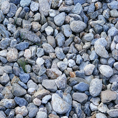
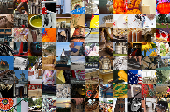
LPIPS (Zhang et al., 2018) makes quality measurements by point-by-point comparisons between deep features from the pre-trained VGG network (Simonyan and Zisserman, 2015). As a result, it cannot properly handle “visual texture,” which is comprised of repeated patterns, subject to some randomization in their location, size, color, and orientation (Portilla and Simoncelli, 2000). DISTS (Ding et al., 2020) provides a better account for texture similarity by identifying a compact set of statistical constraints as global spatial averages of VGG feature maps. When restricted to global texture images (see Fig. 1 (a)), the underlying texture model in DISTS performs well in the analysis-by-synthesis test (Portilla and Simoncelli, 2000) originally advocated by Julesz (Julesz, 1962). However, it is well-known that natural photographic images are composed of “things” (i.e., objects) and “stuff” (i.e., textured surfaces) (Adelson, 2001), localized in space and scale (see Fig. 1 (b)). Therefore, it is desirable to develop structure and texture similarity methods adapted to local image content.

(a)

(b)

Figure 1. Visual comparison between (a) a global texture image and (b) a natural photographic image. We can observe in (b) that texture elements of different visual appearances are distributed at different locations and scales, as indicated by the bounding boxes.

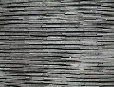
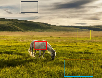
In this paper, we propose a locally adaptive DISTS metric, which we name A-DISTS for full-reference IQA. The central idea is to compute a spatially varying map at a certain scale (i.e., a convolution stage in VGG (Simonyan and Zisserman, 2015)), where each entry indicates the probability of the patch within the receptive field being texture. We identify a single statistical feature, the dispersion index (Cox and Lewis, 1966) computed as the variance-to-mean ratio of convolution responses, which provides an excellent separation between structure and texture patches. The probability map is in turn used to adaptively pool local structure and texture similarity measurements across spatial locations and convolution channels. The resulting A-DISTS is adapted to local image content, and is free of expensive mean opinion scores (MOSs) for supervised training. Our extensive experiments based on ten human-rated IQA databases (Sheikh et al., 2006; Larson and Chandler, 2010; Ponomarenko et al., 2015; Lin et al., 2019; Zhang et al., 2018; Ding et al., 2020; Lai et al., 2016; Ma et al., 2017b; Min et al., 2019; Tian et al., 2018) show that A-DISTS leads to consistent performance improvements in terms of correlation with MOSs, especially on datasets with distortions arising from real-world image restoration applications. Moreover, A-DISTS demonstrates competitive performance in perceptual optimization of single image super-resolution methods.

2. Related Work

This section reviews four full-reference IQA models that are relevant to the proposed A-DISTS: MSE, SSIM (Wang et al., 2004), LPIPS (Zhang et al., 2018), and DISTS (Ding et al., 2020). The former two have made a profound impact on a wide range of multimedia signal processing algorithms, while the later two rely on the same deep feature representation as A-DISTS. All four models have been proven effective in the context of perceptual optimization (Ding et al., 2021).

We use bold capital letters such as $\mathbf{X}$ and $\mathbf{Y}$ to represent input images, bold lower-case letters such as $\mathbf{x}_{k}$ and $\mathbf{y}_{k}$ to represent the $k$th input image patches, and lower-case letters such as $x_{k}$ and $y_{k}$ to represent the $k$th pixel values. Similarly, we use bold capital letters with tildes such as $\tilde{\mathbf{X}}^{(i)}_{j}$ and $\tilde{\mathbf{Y}}^{(i)}_{j}$ to represent the convolution response (i.e., the feature map) from the $j$th channel of the $i$th stage of a DNN (corresponding to $\mathbf{X}$ and $\mathbf{Y}$), bold lower-case letters with tildes such as $\tilde{\mathbf{x}}^{(i)}_{j,k}$ and $\tilde{\mathbf{y}}^{(i)}_{j,k}$ to represent the $k$th feature patches (in $\tilde{\mathbf{X}}^{(i)}_{j}$ and $\tilde{\mathbf{Y}}^{(i)}_{j}$). We denote by $\mathcal{X}$ and $\tilde{\mathcal{X}}$ the image and feature spaces, respectively. We use $f:\mathcal{X}\mapsto\tilde{\mathcal{X}}$ to represent the feature transform which maps an input image to a perceptually plausible representation. It can be the identity mapping (i.e., $\mathbf{X}=\tilde{\mathbf{X}}$) or parameterized by DNNs.

2.1. MSE

MSE is defined as the average of the squares of the errors between the original undistorted image $\mathbf{X}$ and the test “distorted” image $\mathbf{Y}$:

(1) $$\mathrm{MSE}(\mathbf{X},\mathbf{Y})=\frac{1}{K}\sum_{k=1}^{K}\left(x_{k}-y_{k}\right)^{2},$$

where $K$ is the number of pixels in the image. It is simple, physically plausible (e.g., energy preserving according to the Parseval’s theorem), and mathematically beautiful. For example, when MSE is combined with Gaussian source and noise models, the optimal solution in the signal estimation framework is analytical and linear (Wang and Bovik, 2009). One major drawback of MSE and its derivatives is their poor correlation with human perception of image quality.

(a)

(b)

(c)

(d)

(e)

Figure 2. Human perception of visual texture is scale-dependent. (a) - (e): Texture images with increasing scales. Images (a) and (b) allow a relatively small receptive field to capture the intrinsic repetitiveness. In contrast, images (d) and (e) that are composed of small-scale textured surfaces and structural contours require a large receptive field to sufficiently cover the repeated patterns.

2.2. SSIM

SSIM (Wang et al., 2004) is a top-down approach, motivated by the observation that natural photographic images are highly structured. Therefore, a measure of the retention of local image structure should provide a reasonable approximation to perceived image quality. Regardless of various instantiations, the basic form of SSIM measures the similarities of local patch intensities, contrasts, and structures. These are computed using simple patch statistics, and can be combined and simplified to

(2) $$\operatorname{SSIM}(\mathbf{x},\mathbf{y})=l(\mathbf{x},\mathbf{y})\cdot s(\mathbf{x},\mathbf{y})=\left(\frac{2\mu_{\mathbf{x}}\mu_{\mathbf{y}}+c_{1}}{\mu_{\mathbf{x}}^{2}+\mu_{\mathbf{y}}^{2}+c_{1}}\right)\cdot\left(\frac{2\sigma_{\mathbf{x}\mathbf{y}}+c_{2}}{\sigma_{\mathbf{x}}^{2}+\sigma_{\mathbf{y}}^{2}+c_{2}}\right),$$

where $\mu_{\mathbf{x}}$ and $\mu_{\mathbf{y}}$ are (respectively) the mean intensities of $\mathbf{x}$ and $\mathbf{y}$, $\sigma_{\mathbf{x}}^{2}$ and $\sigma_{\mathbf{y}}^{2}$ are (respectively) the variances of $\mathbf{x}$ and $\mathbf{y}$, and $\sigma_{\mathbf{x}\mathbf{y}}$ is the covariance between $\mathbf{x}$ and $\mathbf{y}$. $c_{1}$ and $c_{2}$ are two small positive constants, preventing potential division by zero. The local SSIM values are computed using a sliding window approach, and are averaged spatially to obtain an overall quality score:

(3) $$\operatorname{MSSIM}(\mathbf{X},\mathbf{Y})=\frac{1}{K}\sum_{k=1}^{K}\operatorname{SSIM}(\mathbf{x}_{k},\mathbf{y}_{k}),$$

where we slightly abuse $K$ to denote the number of (overlapping) patches in the image. It is widely acknowledged that SSIM is better at explaining human perceptual data than MSE. Nevertheless, Ding et al. (Ding et al., 2021) found surprisingly that the perceptual gains of the multi-scale version of SSIM (Wang et al., 2003) over MAE are statistically indistinguishable when optimizing four low-level vision tasks.

2.3. LPIPS

LPIPS (Zhang et al., 2018) leverages the “unreasonable” effectiveness of deep features to account for many aspects of human perception, and computes a weighted MSE between normalized feature maps of two images:

(4) $$\operatorname{LPIPS}\left(\mathbf{X},\mathbf{Y}\right)=\sum_{i=1}^{M}\sum_{j=1}^{N_{i}}w_{ij}\operatorname{MSE}\left(\tilde{\mathbf{X}}_{j}^{(i)},\tilde{\mathbf{Y}}_{j}^{(i)}\right),$$

where $w_{ij}\geq 0$ is learnable, indicating the perceptual importance of each channel. $M$ denotes the number of convolution stages, and $N_{i}$ is the number of feature maps in the $i$th stage. LPIPS has multiple configurations, and we adopt the one based on the VGG network (Simonyan and Zisserman, 2015) with weights learned from the BAPPS dataset (Zhang et al., 2018) throughout the paper. It is noteworthy that VGG-based LPIPS can be seen as a generalization of the “perceptual loss” (Johnson et al., 2016), which is widely used in image restoration tasks.

2.4. DISTS

DISTS (Ding et al., 2020) is based on a variant of the VGG network, and makes global SSIM-like structure and texture similarity measurements:

(5) $$\operatorname{DISTS}(\mathbf{X},\mathbf{Y})=1-\sum_{i=0}^{M}\sum_{j=1}^{N_{i}}\left(\alpha_{ij}l\left(\tilde{\mathbf{X}}^{(i)}_{j},\tilde{\mathbf{Y}}^{(i)}_{j}\right)+\beta_{ij}s\left(\tilde{\mathbf{X}}^{(i)}_{j},\tilde{\mathbf{Y}}^{(i)}_{j}\right)\right),$$

where $\{\alpha_{ij},\beta_{ij}\}$ are positive learnable weights, optimized to match human perception of image quality and invariance to resampled texture patches (Ding et al., 2020). Some key modifications of DISTS relative to SSIM and LPIPS are worth mentioning. First, $\ell_{2}$-pooling is adopted to replace the max pooling in the original VGG, which is conducive to de-alias and linearize the intermediate representations (Hénaff and Simoncelli, 2016). Second, the input image is incorporated as an additional feature map (i.e., $\tilde{\mathbf{X}}^{(0)}=\mathbf{X}$) to guarantee the injectivity of the feature transform $f$. Third, unlike Eq. (2), DISTS applies the “texture” similarity function $l(\cdot)$ and the structure similarity function $s(\cdot)$ globally to compare feature maps. It has been empirically proven sensitive to structural distortions and robust to texture substitutions.

3. A-DISTS

In this section, we present in detail the locally adaptive DISTS metric, namely A-DISTS. We first describe the use of the dispersion index to separate structure and texture at different locations and scales. We then compute the final quality score by adaptively weighting local structure and texture measurements.

Structure and Texture Separation. We want to identify robust statistics based on deep representations that are effective in separating structure and texture regions. However, the VGG network (Simonyan and Zisserman, 2015) used in DISTS suffers from the scale ambiguity. That is, we may re-scale a convolution filter by dividing the 3D tensor (and the associated bias term) by an arbitrary non-zero scalar. This can be compensated by re-scaling the next convolution filter connected to it by the same amount without changing the final softmax output. The scale ambiguity arises primarily from the adoption of half-wave rectification (i.e., ReLU) as the nonlinearity. As a consequence, the statistics computed from different convolution responses may be of arbitrary scale. To resolve this, we re-normalize the convolution filters (with size of $\mathrm{height}\times\mathrm{width}\times\mathrm{in\_channel}$) in VGG such that the $\ell_{2}$ norm of each filter is equal to one. With such re-normalization, all convolution filters have responses with similar ranges, making the computed statistics more comparable. Gatys et al. (Gatys et al., 2015) noticed the same issue, and used a different form of re-scaling such that the average response of each filter over spatial locations and channels is equal to one.

(a)

(b)

Figure 3. Sample (a) structure and (b) texture patches of size 128$\times$128 in our image patch dataset manually cropped from the Waterloo Exploration Database (Ma et al., 2017a) and the DIV2K dataset (Timofte et al., 2017).

(a) $\gamma_{\mathbf{x}}^{(1)}$

(b) $\gamma_{\mathbf{x}}^{(2)}$

(c) $\gamma_{\mathbf{x}}^{(3)}$

(d) $\gamma_{\mathbf{x}}^{(4)}$

(e) $\gamma_{\mathbf{x}}^{(5)}$

Figure 4. The conditional histograms (normalized to probabilities) of the dispersion index $\gamma_{\mathbf{x}}^{(i)}$. One can observe that a clear separation between structure and texture at different stages is achieved.

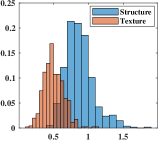
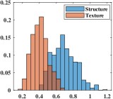
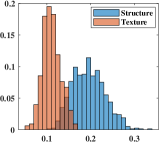
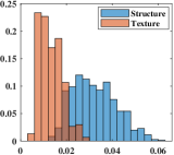
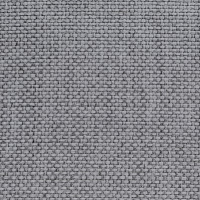
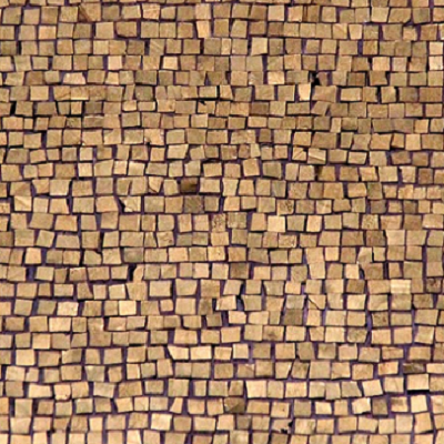
We achieve the discrimination of structure and texture by exploiting two distinct characteristics. First, texture is spatially homogeneous, while structure is more precisely localized in space. Second, the perception of visual texture is scale-dependent. For small-scale visual texture (see Fig. 2 (a) and (b)), a small receptive field (e.g., a $16\times 16$ window) is able to capture its intrinsic repetitiveness, while for large-scale visual texture that is a combination of small-scale textured surfaces and structural contours (see Fig. 2 (d) and (e)), a large receptive field (e.g., a $128\times 128$ window) may be needed to sufficiently cover the repeated patterns. Computationally, we use the dispersion index (Cox and Lewis, 1966) defined by the ratio of variance to mean as the structure/texture indicator. For each stage of VGG, we apply a sliding window approach to compute local dispersion indexes, followed by averaging across channels:

(6) $$\gamma_{\mathbf{x}}^{(i)}=\frac{1}{N_{i}}\sum_{j=1}^{N_{i}}\frac{\left(\sigma_{\tilde{\mathbf{x}}_{j}}^{(i)}\right)^{2}}{\mu_{\tilde{\mathbf{x}}_{j}}^{(i)}+c},$$

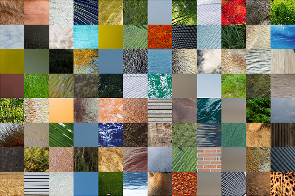
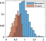
where $\mu_{\tilde{\mathbf{x}}_{j}}^{(i)}$ and $\sigma_{\tilde{\mathbf{x}}_{j}}^{(i)}$ represent (respectively) the mean and standard deviation of the local feature patch $\tilde{\mathbf{x}}^{(i)}_{j}$ in $\tilde{\mathbf{X}}_{j}^{(i)}$. $c$ is a small positive stabilizing constant. The average operation is legitimate due to the re-normalization of the convolution filters in VGG. Intuitively, texture is often under-dispersed compared with structure, leading to a smaller $\gamma_{\mathbf{x}}^{(i)}$. As the receptive field of the VGG increases with the number of convolution and sub-sampling layers, we expect an early-stage $\gamma_{\mathbf{x}}^{(i)}$ is responsive to small-scale texture, while a late-stage $\gamma_{\mathbf{x}}^{(i)}$ is responsible for large-scale texture. To verify this, we gather an image patch dataset, which contains $2,500$ structure patches and $2,500$ texture patches of five different sizes (i.e., $16\times 16$, $32\times 32$, $64\times 64$, $128\times 128$, and $256\times 256$). All patches are cropped from the Waterloo Exploration Database (Ma et al., 2017a) and the DIV2K dataset (Timofte et al., 2017), and manually labeled. Fig. 3 shows sample patches of size $128\times 128$, where we see great variability in structure arrangements and texture appearances. We draw the conditional histograms in Fig. 4, where we find a clear separation between structure and texture at different scales.

(a)

(b)

Figure 5. Illustration of multi-scale texture probability maps. (a): Original image. (b): Texture probability maps with decreasing spatial sizes due to sub-sampling. The warmer the color is, the higher texture probability of the given patch is.

We then feed the dispersion index $\gamma_{\mathbf{x}}^{(i)}$ as a single statistical feature to logistic regression to compute the probability of the given patch being texture:

(7) $$p_{\mathbf{x}}^{(i)}=p\left(``\mathbf{x}\mbox{ is texture}"\mid\gamma_{\mathbf{x}}^{(i)}\right)=\frac{1}{1+e^{-\left(w^{(i)}\gamma_{\mathbf{x}}^{(i)}+b^{(i)}\right)}},$$

where $w^{(i)},b^{(i)}$ are the weight and bias parameters to be fitted on our image patch dataset.

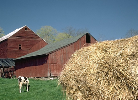
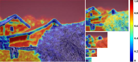
Fig. 5 shows the multi-scale texture probability maps of the “Farm” image, where a warmer color indicates a higher texture probability. Let us focus on the “hay” in the bottom right of the image. When we rely on $\gamma_{\mathbf{x}}^{(1)}$ that uses a small receptive field, the hay is classified as rather isolated structure, as reflected in the probability map at the finest scale. When we increase the receptive field (e.g., using $\gamma_{\mathbf{x}}^{(3)}$ or $\gamma_{\mathbf{x}}^{(4)}$), the hay is identified as texture, where the intrinsic repetitiveness is well captured. If we continue increasing the receptive field, the bottom right region containing the hay is classified towards structure again, which makes perfect sense because the receptive field is large enough to include surrounding structural contours (e.g., the boundaries of the hay and the farmhouse). Other small-scale texture such as the sky, the meadow, and the roof has also been successfully captured by $\gamma_{\mathbf{x}}^{(i)}$ and well reflected in the corresponding probability maps. Similarly, when the receptive field is large enough to include object boundaries, the included texture is part of the structure patch.

Perceptual Distance Metric. With the multi-scale texture probability maps at hand, we are ready to design the spatial pooling strategy for combining local structure and texture similarity measurements. As the proposed quality model is full-reference, we are able to compute two set of probability maps, $\{p_{\mathbf{x}}^{(i)}\}_{i=1}^{5}$ and $\{p_{\mathbf{y}}^{(i)}\}_{i=1}^{5}$ from the VGG representations of the co-located reference and distorted patches, $\mathbf{x}$ and $\mathbf{y}$, respectively. For the purpose of quality assessment, we take the minimum of the two texture probabilities:

(8) $$\tilde{p}^{(i)}=\min\left(p^{(i)}_{\mathbf{x}},p^{(i)}_{\mathbf{y}}\right),$$

which is conductive to penalizing the introduced structural artifacts (e.g., JPEG blocking). For the purpose of perceptual optimization (as described in Section 4.2), we may directly use $p^{(i)}_{\mathbf{x}}$ as weighting to full respect the reference information.

Finally, we define the A-DISTS index as

(9) $$\textrm{A-DISTS}(\mathbf{X},\mathbf{Y})=1-\frac{1}{N}\sum_{i=0}^{M}\sum_{j=1}^{N_{i}}S\left(\tilde{\mathbf{X}}^{(i)}_{j},\tilde{\mathbf{Y}}^{(i)}_{j}\right),$$

and

(10) $$S(\tilde{\mathbf{X}}^{(i)}_{j},\tilde{\mathbf{Y}}^{(i)}_{j})=\frac{1}{K_{i}}\sum_{k=1}^{K_{i}}\left(\tilde{p}_{k}^{(i)}l\left(\tilde{\mathbf{x}}^{(i)}_{j,k},\tilde{\mathbf{y}}^{(i)}_{j,k}\right)+\tilde{q}_{k}^{(i)}s\left(\tilde{\mathbf{x}}^{(i)}_{j,k},\tilde{\mathbf{y}}^{(i)}_{j,k}\right)\right),$$

where $N=\sum_{i=0}^{M}N_{i}$, $\tilde{q}^{(i)}_{k}=1-\tilde{p}^{(i)}_{k}$, and $\tilde{p}^{(i)}_{k}$ is the texture probability of the $k$th patch viewed at the $i$th scale. $l(\cdot)$ and $s(\cdot)$ are defined in Eq. (2). A-DISTS ranges from zero to one, with a higher value indicating poorer predicted quality.

4. Experiments

In this section, we first compare the proposed A-DISTS with a set of full-reference IQA models in term of quality assessment on traditional and novel algorithm-dependent distortions. We then compare A-DISTS against a smaller set of top-performing models in optimization of image super-resolution methods.

Table 1. Performance comparison of A-DISTS against twelve IQA models on four standard IQA databases. Larger PLCC, SRCC, and KRCC numbers represent better performance, with a maximum value of one. Top-$2$ results are highlighted in bold.

Method	LIVE (Sheikh et al., 2006)			CSIQ (Larson and Chandler, 2010)			TID2013 (Ponomarenko et al., 2015)			KADID (Lin et al., 2019)
	PLCC	SRCC	KRCC	PLCC	SRCC	KRCC	PLCC	SRCC	KRCC	PLCC	SRCC	KRCC
PSNR	0.865	0.873	0.680	0.819	0.810	0.601	0.677	0.687	0.496	0.675	0.676	0.488
SSIM (Wang et al., 2004)	0.937	0.948	0.796	0.852	0.865	0.680	0.777	0.727	0.545	0.717	0.724	0.537
MS-SSIM (Wang et al., 2003)	0.940	0.951	0.805	0.889	0.906	0.730	0.830	0.786	0.605	0.820	0.826	0.635
VIF (Sheikh and Bovik, 2006)	0.960	0.964	0.828	0.913	0.911	0.743	0.771	0.677	0.518	0.687	0.679	0.507
MAD (Larson and Chandler, 2010)	0.968	0.967	0.842	0.950	0.947	0.797	0.827	0.781	0.604	0.799	0.799	0.603
FSIMc (Zhang et al., 2011)	0.961	0.965	0.836	0.919	0.931	0.769	0.877	0.851	0.667	0.850	0.854	0.665
GMSD (Xue et al., 2014)	0.957	0.960	0.827	0.945	0.950	0.804	0.855	0.804	0.634	0.845	0.847	0.664
VSI (Zhang et al., 2014)	0.948	0.952	0.806	0.928	0.942	0.786	0.900	0.897	0.718	0.877	0.879	0.691
NLPD (Laparra et al., 2016)	0.932	0.937	0.778	0.923	0.932	0.769	0.839	0.800	0.625	0.811	0.812	0.623
PieAPP (Prashnani et al., 2018)	0.908	0.919	0.750	0.877	0.892	0.715	0.859	0.876	0.683	0.836	0.836	0.647
LPIPS (Zhang et al., 2018)	0.934	0.932	0.765	0.896	0.876	0.689	0.749	0.670	0.497	0.839	0.843	0.653
DISTS (Ding et al., 2020)	0.954	0.954	0.811	0.928	0.929	0.767	0.855	0.830	0.639	0.886	0.887	0.709
A-DISTS (ours)	0.954	0.955	0.812	0.944	0.942	0.796	0.861	0.836	0.642	0.891	0.890	0.715

Table 2. 2AFC score comparison of IQA models on BAPPS and Ding20. It is computed by $r\hat{r}+(1-r)(1-\hat{r})$, where $r$ is the ratio of human votes and $\hat{r}\in\{0,1\}$ is the preference of an IQA model. A higher score indicates better performance.

IQA Model	BAPPS (Zhang et al., 2018)					Ding20 (Ding et al., 2021)
	Color- ization	Video deblurring	Frame interpolation	Super- resolution	All	Denoising	Deblurring	Super- resolution	Compression	All
Human	0.688	0.671	0.686	0.734	0.695	0.761	0.843	0.833	0.891	0.832
PSNR	0.624	0.590	0.543	0.642	0.614	0.627	0.518	0.612	0.689	0.612
SSIM (Wang et al., 2004)	0.522	0.583	0.548	0.613	0.617	0.636	0.575	0.599	0.649	0.615
MS-SSIM (Wang et al., 2003)	0.522	0.589	0.572	0.638	0.596	0.623	0.568	0.655	0.665	0.628
VIF (Sheikh and Bovik, 2006)	0.515	0.594	0.597	0.651	0.603	0.589	0.607	0.655	0.540	0.598
MAD (Larson and Chandler, 2010)	0.490	0.593	0.581	0.655	0.599	0.624	0.671	0.681	0.651	0.657
FSIMc (Zhang et al., 2011)	0.573	0.590	0.581	0.660	0.615	0.522	0.490	0.525	0.563	0.525
GMSD (Xue et al., 2014)	0.517	0.594	0.575	0.676	0.613	0.417	0.454	0.469	0.567	0.477
VSI (Zhang et al., 2014)	0.597	0.591	0.568	0.668	0.622	0.518	0.470	0.487	0.576	0.513
NLPD (Laparra et al., 2016)	0.528	0.584	0.552	0.655	0.600	0.622	0.514	0.629	0.652	0.604
PieAPP (Prashnani et al., 2018)	0.594	0.582	0.598	0.685	0.626	0.625	0.734	0.744	0.822	0.732
LPIPS (Zhang et al., 2018)	0.625	0.605	0.630	0.705	0.641	0.657	0.788	0.768	0.834	0.761
DISTS (Ding et al., 2020)	0.627	0.600	0.625	0.710	0.651	0.602	0.790	0.704	0.833	0.725
A-DISTS (ours)	0.621	0.602	0.616	0.708	0.642	0.629	0.792	0.781	0.846	0.763

4.1. Performance on Quality Assessment

We use three criteria to evaluate the quality assessment performance, including the Pearson linear correlation coefficient (PLCC), the Spearman rank correlation coefficient (SRCC), and the Kendall rank correlation coefficient (KRCC). A four-parameter function is fitted to compensate for a smooth nonlinear relationship when computing PLCC (Ding et al., 2020). Following the practice of SSIM and DISTS, A-DISTS also re-scales the smaller dimension of the test images to $256$ pixels. The size of the sliding window in A-DISTS is $21\times 21$ with a stride of one. We compare A-DISTS with twelve full-reference IQA methods, including nine knowledge-driven models - PSNR, SSIM (Wang et al., 2004), MS-SSIM (Wang et al., 2003), VIF (Sheikh and Bovik, 2006), MAD (Larson and Chandler, 2010), FSIM_c (Zhang et al., 2011), GMSD (Xue et al., 2014), VSI (Zhang et al., 2014), NLPD (Laparra et al., 2016) and three data-driven CNN-based models - PieAPP (Prashnani et al., 2018), LPIPS (Zhang et al., 2018), DISTS (Ding et al., 2020). The implementations of all methods are obtained from the respective authors.

We first show the correlation results on four traditional IQA databases LIVE (Sheikh et al., 2006), CSIQ (Larson and Chandler, 2010), TID2013 (Ponomarenko et al., 2015), and KADID (Lin et al., 2019), consisting of traditional distortion types. The former three datasets have been publicly available for many years, and have been extensively re-used throughout the model design process. Released in 2019, KADID is currently the largest human-rated IQA dataset with $81$ original images and $10,125$ distorted images, respectively. From Table 1, we find that knowledge-driven models (such as MAD (Larson and Chandler, 2010) and FSIM_c (Zhang et al., 2011)) generally perform better on LIVE, CSIQ, and TID2013, but underperform DISTS and the proposed A-DISTS on KADID. This indicates a potential overfitting issue in the field of IQA, arising from excessive hyperparameter tuning and computational module selection. Ding et al. (Ding et al., 2021) obtained a similar result in the context of perceptual optimization. Compared to DISTS as the closest alternative, A-DISTS obtains clear perceptual gains on all four databases measured by all three correlation measures.

Table 3. Performance comparison of IQA models on four image restoration databases.

IQA Model	Liu13 (Liu et al., 2013) (Deblurring)			Ma17 (Ma et al., 2017b) (Super-resolution)			Min19 (Min et al., 2019) (Dehazing)			Tian19 (Tian et al., 2018) (Rendering)
	PLCC	SRCC	KRCC	PLCC	SRCC	KRCC	PLCC	SRCC	KRCC	PLCC	SRCC	KRCC
PSNR	0.807	0.803	0.599	0.611	0.592	0.414	0.754	0.740	0.555	0.605	0.536	0.377
SSIM (Wang et al., 2004)	0.763	0.777	0.574	0.654	0.624	0.440	0.715	0.692	0.513	0.420	0.230	0.156
MS-SSIM (Wang et al., 2003)	0.899	0.898	0.714	0.815	0.795	0.598	0.699	0.687	0.503	0.386	0.396	0.264
VIF (Sheikh and Bovik, 2006)	0.879	0.864	0.672	0.849	0.831	0.638	0.740	0.667	0.504	0.429	0.259	0.173
MAD (Larson and Chandler, 2010)	0.901	0.897	0.714	0.873	0.864	0.669	0.543	0.605	0.437	0.690	0.622	0.441
FSIMc (Zhang et al., 2011)	0.923	0.921	0.749	0.769	0.747	0.548	0.747	0.695	0.515	0.496	0.476	0.324
GMSD (Xue et al., 2014)	0.927	0.918	0.746	0.861	0.851	0.661	0.675	0.663	0.489	0.631	0.479	0.329
VSI (Zhang et al., 2014)	0.919	0.920	0.745	0.736	0.710	0.514	0.730	0.696	0.511	0.512	0.531	0.363
NLPD (Laparra et al., 2016)	0.862	0.853	0.657	0.749	0.732	0.535	0.616	0.608	0.442	0.594	0.463	0.316
PieAPP (Prashnani et al., 2018)	0.752	0.786	0.583	0.791	0.771	0.591	0.749	0.725	0.547	0.352	0.298	0.207
LPIPS (Zhang et al., 2018)	0.853	0.867	0.675	0.809	0.788	0.687	0.825	0.777	0.592	0.387	0.311	0.213
DISTS (Ding et al., 2020)	0.940	0.941	0.784	0.887	0.878	0.697	0.816	0.789	0.600	0.694	0.671	0.485
A-DISTS (ours)	0.943	0.944	0.788	0.905	0.892	0.715	0.831	0.801	0.616	0.705	0.686	0.499

We then compare A-DISTS against the twelve full-reference models on two databases - BAPPS (Zhang et al., 2018) and Ding20 (Ding et al., 2021), composed of processed images by real-world image processing systems. BAPPS (Zhang et al., 2018) is a large-scale patch similarity database with $26,904$ image pairs generated by image colorization, video deblurring, frame interpolation, and super-resolution algorithms. Ding20 (Ding et al., 2021) is a byproduct of a perceptual optimization experiment with $880$ image pairs generated from four low-level vision tasks - image denoising, deblurring, super-resolution, and compression. Since the human opinions are collected in the two-alternative forced choice (2AFC) experiments, the 2AFC score (Zhang et al., 2018), which quantifies the consistency of model predictions relative to human opinions, is employed as the evaluation criterion. Results in Table 2 show that A-DISTS without reliance on human perceptual scores achieves comparable performance to LPIPS, but is slightly inferior to DISTS on BAPPS. We attribute this to the small patch size (i.e., $64\times 64$) of BAPPS, rendering local computation in A-DISTS less effective. For the images with relatively large size in Ding20, A-DISTS outperforms DISTS and the other models.

We also test A-DISTS on another four publicly available image restoration databases with human judgements: Liu13 (Liu et al., 2013), Ma17 (Ma et al., 2017b), Min19 (Min et al., 2019), and Tian19 (Tian et al., 2018), including $1,200$ motion-deblurred images, $1,620$ super-resolved images, $600$ dehazed images, and $140$ rendered images based on depth information, respectively. Table 3 shows the correlation results, where one can observe that A-DISTS is best at explaining human data in these datasets.

In summary, the proposed A-DISTS achieves better correlation performance than DISTS on all ten databases, except for the patch similarity dataset - BAPPS. This provides strong justifications of the key modifications in A-DISTS: structure and texture separation and locally adaptive weighting.

4.2. Performance on Perceptual Optimization

The application scope of objective IQA models is far beyond evaluating image processing algorithms; they can be used as objectives to guide the algorithm design and optimization. In this subsection, we test the gradient-based optimization performance of A-DISTS against four competing models - MAE, MS-SSIM (Wang et al., 2003), LPIPS (Zhang et al., 2018), and DISTS (Ding et al., 2020) in the context of single image super-resolution. We exclude the rest IQA models in Table 1 because they have been empirically shown less competitive on this task (Ding et al., 2021).

Single image super-resolution aims to generate a high-resolution (HR) and high-quality image from a low-resolution (LR) one. In recent years, DNN-based methods (Lim et al., 2017; Wang et al., 2018; Zhang et al., 2019, 2020) have achieved dominant performance on this task. Here, we adopt the Residual in Residual Dense Block (RRDB) network proposed in (Wang et al., 2018) as the backbone to construct our super-resolution algorithms. Training is performed by optimizing a given IQA model:

(11) $$\ell(\bm{\phi})=D\left(f(\mathbf{X}_{l};\bm{\phi}),\mathbf{X}_{h}\right),$$

where $f(\cdot;\bm{\phi})$ denotes the RRDB network parameterized by a vector $\bm{\phi}$. $\mathbf{X}_{h}\in\mathbb{R}^{K}$ is the ground-truth HR image, $\mathbf{X}_{l}\in\mathbb{R}^{\left\lfloor\frac{K}{4^{2}}\right\rfloor}$ is the input LR image down-sampled by a factor of $4$. $D$ represents the IQA metric, with a lower value indicating higher predicted quality.

Figure 6. Sample image pairs in our debiased subjective quality assessment. First column: Reference images. Middle column (form top to bottom): Super-resolved images optimized for MAE, MS-SSIM, LPIPS and DISTS, respectively. Last column : Super-resolved images optimized for A-DISTS. See text for more details on image selection.

(a)

(b)

(c)

(d)

(e)

(f)

(g)

(h)

(i)

(j)

(k)

(l)

(a) Original

(b) MAE

(c) MS-SSIM

(d) LPIPS

(e) DISTS

(f) A-DISTS

Figure 7. Super-resolution results of three example images optimized for different IQA models.

We use the DIV2K database (Timofte et al., 2017) and the Waterloo Exploration Database (Ma et al., 2017a) for training and testing, respectively. We generate LR images by downsampling HR images with bicubic interpolation. Following the practice of (Ding et al., 2021), the model parameters optimized for MAE are employed as the initializations for the networks to be optimized by other models. More training details (e.g., optimizer, learning rate, batch size, etc.) are inherited from (Wang et al., 2018). We apply the trained networks to the test images, and conduct a subjective user study for quantitative evaluation. To ensure a fair comparison (i.e., to avoid potential cherry-picking test results), we adopt the debiased subjective assessment method in (Cao et al., 2021), which automatically samples a small set of adaptive and diverse test images by solving

(12) $$\mathbf{X}^{\star}=\operatorname*{argmax}_{\mathbf{X}_{l}\in\mathcal{X}}~{}\bar{D}(f_{i}(\mathbf{X}_{l}),f_{j}(\mathbf{X}_{l})),\quad 1\leq i\leq j\leq 5,$$

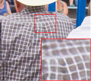
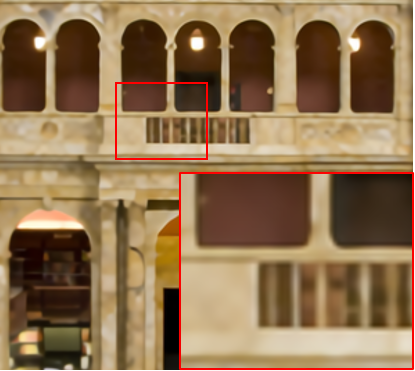
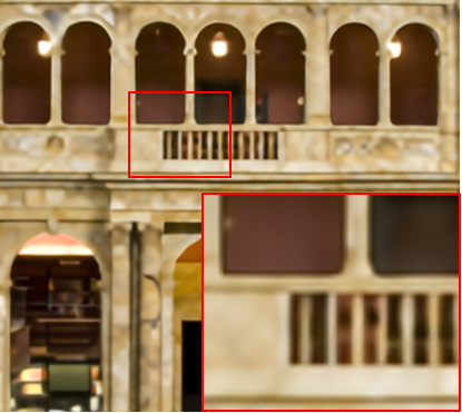
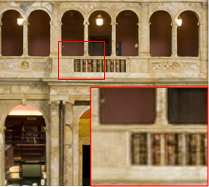
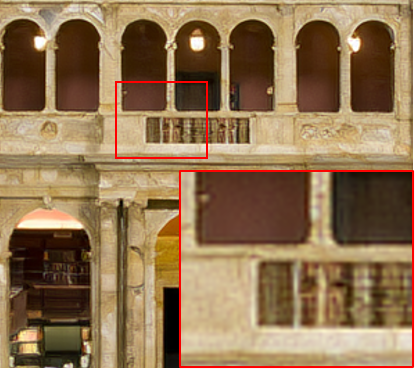
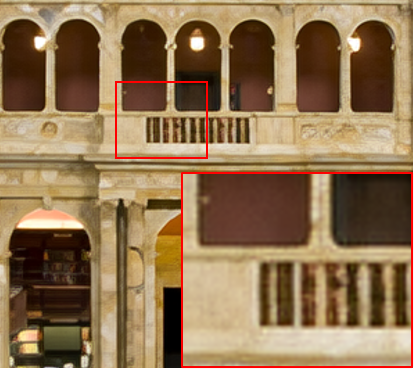
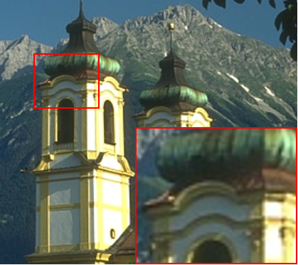
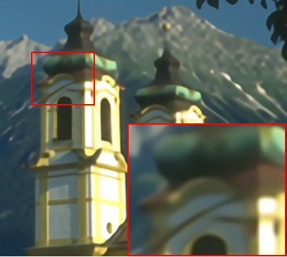
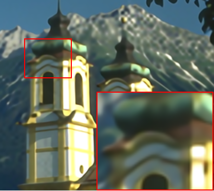
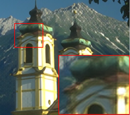
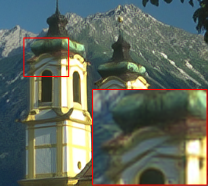
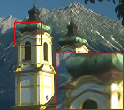
where $\mathcal{X}$ denotes the set of LR images from the Waterloo Exploration Database (Ma et al., 2017a). $i$ and $j$ are the algorithm indices. $\bar{D}$ is a measure to approximate the perceptual distance between the super-resolved images $f_{i}(\mathbf{X}_{l})$ and $f_{j}(\mathbf{X}_{l})$. We define $\bar{D}$ as the average of two IQA models $D_{i}$ and $D_{j}$ used to optimize $f_{i}$ and $f_{j}$, respectively. By adding a diversity term (Cao et al., 2021), we are able to automatically select a small subset of images in $\mathcal{X}$ that best differentiate between two networks $f_{i}$ and $f_{j}$. The comparison is exhausted for all $\binom{5}{2}$ pairs of algorithms. Fig. 6 shows several sample image pairs in our debiased subjective quality assessment experiment.

Table 4. Global ranking of the five IQA models for use in optimizing single image super-resolution methods in the debiased subjective testing (Cao et al., 2021). A higher ranking score indicates better performance.

IQA model	MAE	MS-SSIM	LPIPS	DISTS	A-DISTS
Ranking score	-1.524	-1.453	0.762	0.980	1.095

We employ the 2AFC method for subjective rating. For each algorithm pair, we set $20$ images according to Eq. (12). This leads to a total of $\binom{5}{2}\times 20=200$ paired comparisons for $5$ IQA models. Subjects are required to choose the image with higher perceived quality with reference to the ground-truth image. Subjects are allowed to adjust the viewing distance and zoom in/out any part of the images for careful inspection. We gather data from $20$ subjects with general background knowledge of multimedia signal processing. The Bradley–Terry model (Bradley and Terry, 1952) is adopted to convert paired comparison results to a global ranking, as shown in Table 4. We find that the proposed A-DISTS achieves the best perceptual optimization results on average. The ranking of the remaining models is consistent with the conclusions in (Ding et al., 2021).

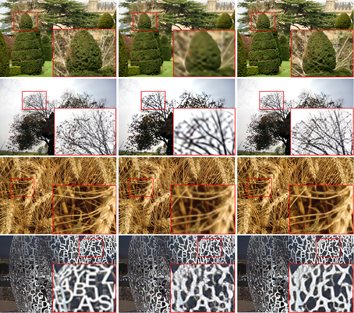
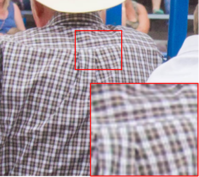
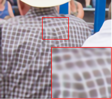
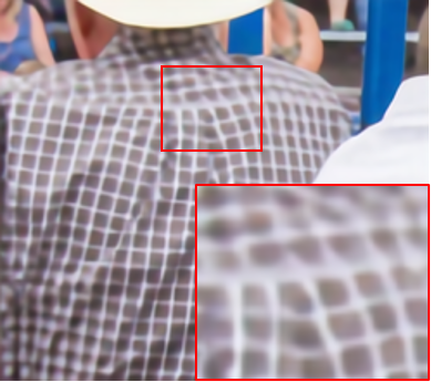
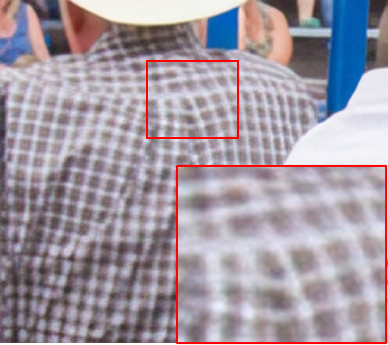
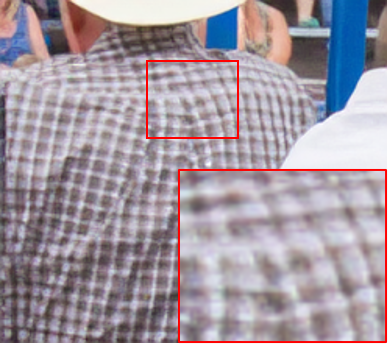
Fig. 7 shows three visual examples of super-resolution methods optimized for different IQA models. Like many other studies, we find MAE and MS-SSIM encourage blurry images. The results by DISTS are generally sharper, but appear distortions in structure regions and noise in texture regions. With locally adaptive structure and texture similarity measurements, A-DISTS generates better visual results with reduced structural artifacts and more plausible textures.

5. Conclusion and Discussion

We have developed a locally adaptive structure and texture similarity index for full-reference IQA. The keys to the success of our approach are 1) the separation of structure and texture across space and scale and 2) the adaptive weighting of quality measurements according to local image content. A-DISTS is free of expensive MOSs for supervised training, correlates well with human data in standard IQA and image restoration databases, and demonstrates competitive optimization performance for single image super-resolution.

One limitation of the proposed A-DISTS is that the performance on global texture-related tasks may be slightly compromised. For example, on the SynTEX database (Golestaneh et al., 2015) for texture similarity, A-DISTS obtains an SRCC of $0.760$ compared to $0.923$ by DISTS. Therefore, a generalized quality measure that translates in a content-dependent way from DISTS to A-DISTS is worth deeper investigation. Nevertheless, as most natural photographic images are made of “things and stuff”, we believe the proposed A-DISTS holds much promise for use in a wide range of real-world image processing applications.

References

- (1)
- Adelson (2001) Edward H. Adelson. 2001. On seeing stuff: The perception of materials by humans and machines. In SPIE Human Vision and Electronic Imaging. 1–12.
- Bosse et al. (2018) Sebastian Bosse, Dominique Maniry, Klaus-Robert Müller, Thomas Wiegand, and Wojciech Samek. 2018. Deep neural networks for no-reference and full-reference image quality assessment. IEEE Transactions on Image Processing 27, 1 (2018), 206–219.
- Bradley and Terry (1952) Ralph Allan Bradley and Milton E. Terry. 1952. Rank analysis of incomplete block designs: I. The method of paired comparisons. Biometrika 39, 3/4 (1952), 324–345.
- Cao et al. (2021) Peibei Cao, Zhangyang Wang, and Kede Ma. 2021. Debiased subjective assessment of real-world image enhancement. In IEEE Conference on Computer Vision and Pattern Recognition.
- Cox and Lewis (1966) D. R. Cox and P. A. W Lewis. 1966. The statistical analysis of series of events. The Mathematical Gazette 51, 377 (1966), 266–267.
- Ding et al. (2020) Keyan Ding, Kede Ma, Shiqi Wang, and Eero P. Simoncelli. 2020. Image quality assessment: Unifying structure and texture similarity. IEEE Transactions on Pattern Analysis and Machine Intelligence (2020).
- Ding et al. (2021) Keyan Ding, Kede Ma, Shiqi Wang, and Eero P. Simoncelli. 2021. Comparison of full-reference image quality models for optimization of image processing systems. International Journal of Computer Vision 129 (2021), 1258–1281.
- Duanmu et al. (2021) Zhengfang Duanmu, Wentao Liu, Zhongling Wang, and Zhou Wang. 2021. Quantifying visual image quality: A Bayesian view. Annual Review of Vision Science (2021).
- Gatys et al. (2015) Leon Gatys, Alexander S Ecker, and Matthias Bethge. 2015. Texture synthesis using convolutional neural networks. In Conference on Neural Information Processing Systems. 262–270.
- Golestaneh et al. (2015) S Alireza Golestaneh, Mahesh M Subedar, and Lina J Karam. 2015. The effect of texture granularity on texture synthesis quality. In Applications of Digital Image Processing XXXVIII, Vol. 9599. 356 – 361.
- Hénaff and Simoncelli (2016) Olivier J Hénaff and Eero P Simoncelli. 2016. Geodesics of learned representations. In International Conference on Learning Representations. 1–10.
- Johnson et al. (2016) Justin Johnson, Alexandre Alahi, and Fei-Fei Li. 2016. Perceptual losses for real-time style transfer and super-resolution. In European Conference on Computer Vision. 694–711.
- Julesz (1962) Bela Julesz. 1962. Visual pattern discrimination. IRE Transactions on Information Theory 8, 2 (1962), 84–92.
- Lai et al. (2016) Wei-Sheng Lai, Jia-Bin Huang, Zhe Hu, Narendra Ahuja, and Ming-Hsuan Yang. 2016. A comparative study for single image blind deblurring. In IEEE Conference on Computer Vision and Pattern Recognition. 1701–1709.
- Laparra et al. (2016) Valero Laparra, Johannes Ballé, Alexander Berardino, and Eero P Simoncelli. 2016. Perceptual image quality assessment using a normalized Laplacian pyramid. Electronic Imaging 2016, 16 (2016), 1–6.
- Larson and Chandler (2010) Eric C. Larson and Damon M. Chandler. 2010. Most apparent distortion: Full-reference image quality assessment and the role of strategy. Journal of Electronic Imaging 19, 1 (2010), 1–21.
- Lim et al. (2017) Bee Lim, Sanghyun Son, Heewon Kim, Seungjun Nah, and Kyoung Mu Lee. 2017. Enhanced deep residual networks for single image super-resolution. In IEEE Conference on Computer Vision and Pattern Recognition Workshop. 136–144.
- Lin et al. (2019) Hanhe Lin, Vlad Hosu, and Dietmar Saupe. 2019. KADID-10k: A large-scale artificially distorted IQA database. In IEEE International Conference on Quality of Multimedia Experience. 1–3.
- Liu et al. (2013) Yiming Liu, Jue Wang, Sunghyun Cho, Adam Finkelstein, and Szymon Rusinkiewicz. 2013. A no-reference metric for evaluating the quality of motion deblurring. ACM Transactions on Graphics 32, 6 (2013), 175:1–175:12.
- Ma et al. (2017b) Chao Ma, Chih-Yuan Yang, Xiaokang Yang, and Ming-Hsuan Yang. 2017b. Learning a no-reference quality metric for single-image super-resolution. Computer Vision and Image Understanding 158 (2017), 1–16.
- Ma et al. (2017a) Kede Ma, Zhengfang Duanmu, Qingbo Wu, Zhou Wang, Hongwei Yong, Hongliang Li, and Lei Zhang. 2017a. Waterloo exploration database: New challenges for image quality assessment models. IEEE Transactions on Image Processing 26, 2 (2017), 1004–1016.
- Min et al. (2019) Xiongkuo Min, Guangtao Zhai, Ke Gu, Yucheng Zhu, Jiantao Zhou, Guodong Guo, Xiaokang Yang, Xinping Guan, and Wenjun Zhang. 2019. Quality evaluation of image dehazing methods using synthetic hazy images. IEEE Transactions on Multimedia 21, 9 (2019), 2319–2333.
- Ponomarenko et al. (2015) Nikolay Ponomarenko, Lina Jin, Oleg Ieremeiev, Vladimir Lukin, Karen Egiazarian, Jaakko Astola, Benoit Vozel, Kacem Chehdi, Marco Carli, Federica Battisti, and C.-C. Jay Kuo. 2015. Image database TID2013: Peculiarities, results and perspectives. Signal Processing Image Communication 30 (2015), 57–77.
- Portilla and Simoncelli (2000) Javier Portilla and Eero P. Simoncelli. 2000. A parametric texture model based on joint statistics of complex wavelet coefficients. International Journal of Computer Vision 40, 1 (2000), 49–70.
- Prashnani et al. (2018) Ekta Prashnani, Hong Cai, Yasamin Mostofi, and Pradeep Sen. 2018. PieAPP: Perceptual image-error assessment through pairwise preference. In IEEE Conference on Computer Vision and Pattern Recognition. 1808–1817.
- Sheikh and Bovik (2006) Hamid R. Sheikh and Alan C. Bovik. 2006. Image information and visual quality. IEEE Transactions on Image Processing 15, 2 (2006), 430–444.
- Sheikh et al. (2006) Hamid R. Sheikh, Zhou Wang, Alan C. Bovik, and Lawrence Cormack. 2006. Image and video quality assessment research at LIVE. [Online]. Available: http://live.ece.utexas.edu/research/quality/.
- Simonyan and Zisserman (2015) Karen Simonyan and Andrew Zisserman. 2015. Very deep convolutional networks for large-scale image recognition. In International Conference on Learning Representations. 1–14.
- Tian et al. (2018) Shishun Tian, Lu Zhang, Luce Morin, and Olivier Déforges. 2018. A benchmark of DIBR synthesized view quality assessment metrics on a new database for immersive media applications. IEEE Transactions on Multimedia 21, 5 (2018), 1235–1247.
- Timofte et al. (2017) Radu Timofte, Eirikur Agustsson, Luc Van Gool, Ming-Hsuan Yang, and Lei Zhang. 2017. NTIRE 2017 challenge on single image super-resolution: Methods and results. In IEEE Conference on Computer Vision and Pattern Recognition. 114–125.
- Wang et al. (2018) Xintao Wang, Ke Yu, Shixiang Wu, Jinjin Gu, Yihao Liu, Chao Dong, Yu Qiao, and Chen Change Loy. 2018. ESRGAN: Enhanced super-resolution generative adversarial networks. In European Conference on Computer Vision Workshops. 1–16.
- Wang (2016) Zhou Wang. 2016. Objective image quality assessment: Facing the real-world challenges. Electronic Imaging 2016, 13 (2016), 1–6.
- Wang and Bovik (2009) Zhou Wang and Alan C. Bovik. 2009. Mean squared error: Love it or leave it? A new look at signal fidelity measures. IEEE Signal Processing Magazine 26, 1 (2009), 98–117.
- Wang et al. (2004) Zhou Wang, Alan C. Bovik, Hamid R. Sheikh, and Eero P. Simoncelli. 2004. Image quality assessment: From error visibility to structural similarity. IEEE Transactions on Image Processing 13, 4 (2004), 600–612.
- Wang et al. (2003) Zhou Wang, Eero P. Simoncelli, and Alan C. Bovik. 2003. Multiscale structural similarity for image quality assessment. In IEEE Asilomar Conference on Signals, System and Computers. 1398–1402.
- Watson (2000) Andrew B Watson. 2000. Visual detection of spatial contrast patterns: Evaluation of five simple models. Optics Express 6, 1 (2000), 12–33.
- Xue et al. (2014) Wufeng Xue, Lei Zhang, Xuanqin Mou, and Alan C. Bovik. 2014. Gradient magnitude similarity deviation: A highly efficient perceptual image quality index. IEEE Transactions on Image Processing 23, 2 (2014), 684–695.
- Zhang et al. (2020) Kai Zhang, Luc Van Gool, and Radu Timofte. 2020. Deep unfolding network for image super-resolution. In IEEE Conference on Computer Vision and Pattern Recognition. 3217–3226.
- Zhang et al. (2014) Lin Zhang, Ying Shen, and Hongyu Li. 2014. VSI: A visual saliency-induced index for perceptual image quality assessment. IEEE Transactions on Image Processing 23, 10 (2014), 4270–4281.
- Zhang et al. (2011) Lin Zhang, Lei Zhang, Xuanqin Mou, and David Zhang. 2011. FSIM: A feature similarity index for image quality assessment. IEEE Transactions on Image Processing 20, 8 (2011), 2378–2386.
- Zhang et al. (2018) Richard Zhang, Phillip Isola, Alexei A Efros, Eli Shechtman, and Oliver Wang. 2018. The unreasonable effectiveness of deep features as a perceptual metric. In IEEE Conference on Computer Vision and Pattern Recognition. 586–595.
- Zhang et al. (2019) Wenlong Zhang, Yihao Liu, Chao Dong, and Yu Qiao. 2019. RankSRGAN: Generative adversarial networks with ranker for image super-resolution. In IEEE Conference on Computer Vision and Pattern Recognition. 3096–3105.