Boundedness from below of $SU(n)$ potentials

Abstract

Vacuum stability requires that the scalar potential is bounded from below. Whether or not this is true depends on the scalar quartic interactions alone, but even so the analysis is arduous and has only been carried out for a limited set of models. Complementing the existing literature, this work contains the necessary and sufficient conditions for two $SU(n)$ invariant potentials to be bounded from below. In particular, expressions are given for models with the fundamental and the 2-index (anti)symmetric representations of this group. A sufficient condition for vacuum stability is also provided for models with the fundamental and the adjoint representations. Finally, some considerations are made concerning the model with the gauge group $SU(2)$ and the scalar representations $\boldsymbol{1}$, $\boldsymbol{2}$ and $\boldsymbol{3}$; such a setup is particularly important for neutrino mass generation and lepton number violation.

1 Introduction

The study of scalar potentials can be a formidable task given that these are quartic functions of several variables. Despite the difficulty, their analysis is crucial as the scalar minima correspond to the possible vacuum configurations.

A given vacuum state cannot be absolutely stable if the scalar potential acquires lower values for some other choice of field values. Of particular concern are those cases where the potential is not bounded from below (BFB), meaning that it acquires arbitrarily large negative values. If this were to happened it would be for field values far from the origin, in which case quadratic and trilinear interactions can be neglected. Even so, deriving the BFB conditions quickly becomes a very complicated problem as the number of scalar fields increases, so much so that in the literature one can find the derivation of these conditions for just a few models. Among the cases which were considered there is the two Higgs doublet model [1], the type-II seesaw potential with the Higgs doublet plus an $SU(2)$ triplet [2, 3], special three Higgs doublet models [4, 5, 6] and also an $SU(3)$ invariant potential with three triplets [7]. Several other works have analyzed the vacuum stability of specific models or discussed general techniques for doing so [8, 9, 10, 11].

Of particular relevance to the following discussion is the analysis in reference [3] on the BFB conditions for the Standard Model potential with the inclusion of a scalar triplet, which refined the results in [2]. This corresponds to an $SU(2)$ invariant potential with the scalar representations $\boldsymbol{2}$ and $\boldsymbol{3}$. Following up on that analysis, the aim of the present work is threefold:

1. Generalize the results of [3] to $SU(n)$ invariant potentials with the fundamental representation plus a 2-index representation — the symmetric, the antisymmetric or the adjoint. This last representation presents a unique difficulty, hence I will only derive a sufficient condition (which is not a necessary one) for the potential to be bounded from below.

2. A crucial step in the derivation of the BFB conditions in [3] — namely the shape of figure 1 — was not demonstrated explicitly up to now, as it was obtained via elaborate manipulations of expressions in a computer. In this work I provide a fully analytical understanding of these calculations.

3. The Standard Model potential supplemented by a scalar singlet and a scalar triplet (a 1-2-3 $SU(2)$ potential, in reference to the sizes of the irreducible fields) is important in the context of neutrino mass generation, and also lepton number violation [12]. For such a complicated potential, instead of providing in full generality the BFB conditions which are both necessary and sufficient, I will derive them for an important special case where one of the quartic couplings is neglected. Furthermore, a sufficient condition will be given for the general case.

It is worth pointing out that extending the results of [3] to $SU(n)$, with $n>2$, is not a mere mathematical curiosity. Indeed, it is plausible that the fundamental laws of physics are symmetric under a group larger than the Standard Model one, such as $SU(3)\times SU(3)\times U(1)$ [13, 14, 15, 16], $SU(4)\times SU(2)\times SU(2)$ [17], $SU(5)$ [18] and even bigger special unitary groups (see for instance [19] and the references contained therein). The viability of the associated models requires several irreducible scalar representations, in some cases coinciding with the ones analyzed in this work [20]. In other cases, such as the Georgi-Glashow $SU(5)$ model [18], the field content studied in this work is just part of the full scalar sector, and if so the conditions presented here are still applicable — they are necessary (but not sufficient) for the potential to be bounded from below.

The rest of this document is structured as follows. Section 2 introduces and analyzes the $SU(n)$ invariant scalar potential with a fundamental and a 2-index symmetric representation. The BFB conditions depend on two crucial parameters, $\alpha$ and $\beta$, which are considered in detail in section 3 plus an appendix. With a thorough understanding of them, in section 4 I derive the BFB conditions for the potential mentioned in section 2 with a 2-index symmetric representation. Some modifications are necessary in the case of a 2-index anti-symmetric representation, as explained in section 5. One can also find there an analysis of the more complicated setup where the 2-index representation is the adjoint. The 1-2-3 model mentioned earlier is considered in section 6. Finally, for the reader’s convenience, a summary of the results can be found at the very end.

2 An $SU(n)$ invariant potential

Consider a scalar $\phi_{i}$ transforming under the fundamental representation of $SU(n)$ as well as a $\Delta_{ij}$ transforming under the 2-index symmetric representation of this group. These fields can be viewed as a vector and a matrix which change under an $SU(n)$ transformation $U$ as follows:

$$\phi\rightarrow U\phi\,,$$ (1)

$$\Delta\rightarrow U\Delta U^{T}\,.$$ (2)

There are 5 quartic terms allowed by the symmetry, which are

$$V^{(4)} =\frac{\lambda_{\phi}}{2}\left(\phi^{\dagger}\phi\right)^{2}+\frac{\lambda_{\Delta}}{2}\left[\textrm{Tr}\left(\Delta\Delta^{*}\right)\right]^{2}+\frac{\lambda_{\Delta}^{\prime}}{2}\textrm{Tr}\left(\Delta\Delta^{*}\Delta\Delta^{*}\right)+\lambda_{\phi\Delta}\left(\phi^{\dagger}\phi\right)\textrm{Tr}\left(\Delta\Delta^{*}\right)+\lambda_{\phi\Delta}^{\prime}\phi^{\dagger}\Delta\Delta^{*}\phi\,.$$ (3)

The field $\Delta$ has $n(n+1)/2$ independent components, but it is always possible to cast $\Delta$ in a diagonal form $\textrm{diag}\left(\Delta_{1},\Delta_{2},\cdots,\Delta_{n}\right)$ with a gauge transformation. In this basis, the quartic potential reads

$$V^{(4)} =\frac{\lambda_{\phi}}{2}\left(\sum_{i}\left|\phi_{i}\right|^{2}\right)^{2}+\frac{\lambda_{\Delta}}{2}\left(\sum_{i}\left|\Delta_{i}\right|^{2}\right)^{2}+\frac{\lambda_{\Delta}^{\prime}}{2}\sum_{i}\left|\Delta_{i}\right|^{4}$$

$$+\lambda_{\phi\Delta}\left(\sum_{i}\left|\phi_{i}\right|^{2}\right)\left(\sum_{i}\left|\Delta_{i}\right|^{2}\right)+\lambda_{\phi\Delta}^{\prime}\sum_{i}\left|\phi_{i}\right|^{2}\left|\Delta_{i}\right|^{2}\,.$$ (4)

The above expression depends only on the $2n$ non-negative variables $\left|\phi_{i}\right|^{2}$ and $\left|\Delta_{i}\right|^{2}$, and the dependence is quadratic. Hence one can in principle use the co-positivity conditions [8] for a $2n$-dimensional matrix to infer the values of the $\lambda$ parameters for which $V^{(4)}$ is always positive. The problem is that these conditions become quite complicated for square matrices with 4 or more rows. I will therefore follow an approach in line with [3] which is more readily applicable to variable $n$’s.

Note that with a rescaling

$$\left|\phi_{i}\right|^{2}\rightarrow\frac{1}{\sqrt{\lambda_{\phi}}}\left|\widetilde{\phi}_{i}\right|^{2}$$ (5)

$$\left|\Delta_{i}\right|^{2}\rightarrow\frac{1}{\sqrt{\lambda_{\Delta}+\lambda_{\Delta}^{\prime}}}\left|\widetilde{\Delta}_{i}\right|^{2}$$ (6)

one can deduce that whether or not the potential is bounded from below must depend on the 5 $\lambda$’s only through the 3 combinations

$$\kappa_{\Delta}^{\prime}\equiv\frac{\lambda_{\Delta}^{\prime}}{\lambda_{\Delta}+\lambda_{\Delta}^{\prime}}\,,\;\kappa_{\phi\Delta}\equiv\frac{\lambda_{\phi\Delta}}{\sqrt{\lambda_{\phi}}\sqrt{\lambda_{\Delta}+\lambda_{\Delta}^{\prime}}}\,,\;\kappa_{\phi\Delta}^{\prime}\equiv\frac{\lambda_{\phi\Delta}^{\prime}}{\sqrt{\lambda_{\phi}}\sqrt{\lambda_{\Delta}+\lambda_{\Delta}^{\prime}}}\,$$ (7)

plus the signs of $\lambda_{\phi}$ and $\lambda_{\Delta}+\lambda_{\Delta}^{\prime}$, which need to be positive. Indeed, to check that this last statement is true it suffices to consider the specific field directions where only $\phi_{1}$ is non-zero, and also the case when only $\Delta_{1}$ is non-zero. Despite the allure of working with only 3 $\kappa$’s, I will not use these them in the following discussion.

Let us now introduce the variables

$$\alpha\equiv\frac{\sum_{i}\left|\Delta_{i}\right|^{4}}{\left(\sum_{i}\left|\Delta_{i}\right|^{2}\right)^{2}}\textrm{ and }\beta\equiv\frac{\sum_{i}\left|\Delta_{i}\right|^{2}\left|\phi_{i}\right|^{2}}{\left(\sum_{i}\left|\Delta_{i}\right|^{2}\right)\left(\sum_{i}\left|\phi_{i}\right|^{2}\right)}$$ (8)

so that

$$V^{(4)} =\frac{1}{2}\left(\begin{array}[]{c}\sum_{i}\left|\phi_{i}\right|^{2}\\ \sum_{i}\left|\Delta_{i}\right|^{2}\end{array}\right)^{T}\left(\begin{array}[]{cc}\lambda_{\phi}&\lambda_{\phi\Delta}+\beta\lambda_{\phi\Delta}^{\prime}\\ \lambda_{\phi\Delta}+\beta\lambda_{\phi\Delta}^{\prime}&\lambda_{\Delta}+\alpha\lambda_{\Delta}^{\prime}\end{array}\right)\left(\begin{array}[]{c}\sum_{i}\left|\phi_{i}\right|^{2}\\ \sum_{i}\left|\Delta_{i}\right|^{2}\end{array}\right)$$ (15)

This expression is positive if and only if for all values of $\alpha$ and $\beta$ the $2\times 2$ matrix above is co-positive. In turn, that is true if and only if

$$\lambda_{\phi}>0\;\textrm{ and }\lambda_{\Delta}+\alpha\lambda_{\Delta}^{\prime}>0\;\textrm{ and }\lambda_{\phi\Delta}+\beta\lambda_{\phi\Delta}^{\prime}+\sqrt{\lambda_{\phi}\left(\lambda_{\Delta}+\alpha\lambda_{\Delta}^{\prime}\right)}>0\,$$ (16)

for all values of $\alpha$ and $\beta$. With rather straightforward steps, we have reduced the initial problem, with $n+n\left(n+1\right)/2$ field directions, first down to $2n$ variables (the $\left|\phi_{i}\right|^{2}$ and the $\left|\Delta_{i}\right|^{2}$) and eventually down to just two ($\alpha$ and $\beta$). However, to get rid of these remaining field-dependent quantities, we must first understand what is the range of values they can take.

3 The allowed values of $\alpha$ and $\beta$

The price to pay for reducing the $2n$ non-negative field quantities $\left|\phi_{i}\right|^{2}$ and $\left|\Delta_{i}\right|^{2}$ to just $\alpha$ and $\beta$ is that the range of the new variable is not obvious. It is rather easy to see that $\max\left(\alpha\right)=1$ when just one $\left|\Delta_{i}\right|^{2}$ is different from zero, while on the other hand $\min\left(\alpha\right)=1/n$ is reached when all $\left|\Delta_{i}\right|^{2}$ have a constant value. As for $\beta$, if just a single $\phi_{i}$ is different from zero, and the same is true for the corresponding $\Delta_{i}$ ($\Delta_{j\neq i}=0$) then we reach a maximum $\beta$ value of 1. If on the other hand a single $\phi_{i}$ is different from zero and only one $\Delta_{j\neq i}$ is non-null, then $\beta$ reaches a minimum of 0.

So $\alpha\in\left[1/n,1\right]$ and $\beta\in\left[0,1\right]$. Nevertheless the allowed region for $\left(\alpha,\beta\right)$ is not a rectangle. For example, when $\alpha$ is minimal ($=1/n$), all the $\left|\Delta_{i}\right|^{2}$ must have the same value $c$ which means that $\beta$ is forced to be $c\left(\sum_{i}\left|\phi_{i}\right|^{2}\right)/\left[\left(\sum_{i}\left|\phi_{i}\right|^{2}\right)nc\right]=1/n$ as well.

The border of the allowed area for $\left(\alpha,\beta\right)$ can be found following a generic method proposed long ago in [21, 22]. These two quantities can be seen as functions of the variables $\left|\phi_{i}\right|^{2}$ plus the $\left|\Delta_{i}\right|^{2}$, and at the border the vectors $\left(\partial\alpha/\partial\left|\phi_{i}\right|^{2},\partial\beta/\partial\left|\phi_{i}\right|^{2}\right)^{T}$ and $\left(\partial\alpha/\partial\left|\Delta_{j}\right|^{2},\partial\beta/\partial\left|\Delta_{j}\right|^{2}\right)^{T}$ for all $i$ and $j$ must be proportional to each other (the null vector $\left(0,0\right)^{T}$ is allowed as well). That is because at the border of the allowed area for $\left(\alpha,\beta\right)$ it should not be possible to move in two independent directions in the $\left(\alpha,\beta\right)$ plane by making small variations of the $\left|\phi_{i}\right|^{2}$ and the $\left|\Delta_{i}\right|^{2}$. The only caveat is that these last variables cannot be negative, hence for $\left|\phi_{i}\right|^{2}=0$ and for $\left|\Delta_{i}\right|^{2}=0$ the previous restriction does not apply. Such nuance can be taken into account by saying that the $2n$ vectors

$$\left|\phi_{j}\right|^{2}\left(\partial\alpha/\partial\left|\phi_{j}\right|^{2},\partial\beta/\partial\left|\phi_{j}\right|^{2}\right)^{T}=x_{j}\left(0,y_{j}-\beta\right)^{T}$$ (17)

and

$$\left|\Delta_{k}\right|^{2}\left(\partial\alpha/\partial\left|\Delta_{k}\right|^{2},\partial\beta/\partial\left|\Delta_{k}\right|^{2}\right)^{T}=y_{k}\left(2\left(y_{k}-\alpha\right),x_{k}-\beta\right)^{T}$$ (18)

must either be null or proportional to some constant vector. The notation $x_{j}\equiv\left|\phi_{j}\right|^{2}/\sum_{i}\left|\phi_{i}\right|^{2}$ and $y_{j}\equiv\left|\Delta_{j}\right|^{2}/\sum_{i}\left|\Delta_{i}\right|^{2}$ was used to reduce the complexity of the expressions (note that by definition $\sum_{i}x_{i}=\sum_{i}y_{i}=1$). It is straightforward but tedious to carefully go through all cases in which the above vectors are all aligned with each other, or null. Therefore a description of the various possibilities is relegated to the appendix.

The conclusion of the discussion contained therein is that the allowed values of $\left(\alpha,\beta\right)$ correspond to the shaded area in figure 1, including the border lines. Note that — as expected — this shape grows with $n$ since the $SU(n)$-invariant potential can be seen as a special case of the $SU(n+1)$-invariant where some field components are set to zero. As a consequence, the BFB conditions on the $\lambda$’s become more stringent as $n$ increases. Of particular relevance is the lower part of this shape, which is defined by the quadratic relation

$$\alpha=\frac{1-2\beta+n\beta^{2}}{n-1}\,.$$ (19)

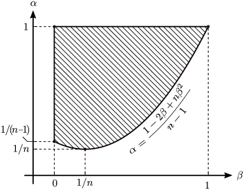
Figure 1: Allowed values of the important parameters $\alpha$ and $\beta$, defined in equation (8), when $\Delta$ is symmetric.

The figure shown without proof in [3] corresponds to the special situation where $n=2$, in which case the allowed region for $\left(\alpha,\beta\right)$ is symmetric under reflection around the vertical axis $\beta=1/2$; for $n>2$ there is a qualitative change as the point $\left(\beta,\alpha\right)=\left(0,1/\left(n-1\right)\right)$ becomes distinct from $\left(0,1\right)$.

4 The conditions for the $\lambda$’s

We may now return to the inequalities in (16). Since they must hold for all $\alpha$ and $\beta$, substituting $\alpha$ in $\lambda_{\Delta}+\alpha\lambda_{\Delta}^{\prime}>0$ by the smallest ($1/n$) and the largest (1) values this variable can take, we conclude that this last inequality is equivalent to

$$n\lambda_{\Delta}+\lambda_{\Delta}^{\prime}>0\textrm{ and }\lambda_{\Delta}+\lambda_{\Delta}^{\prime}>0\,.$$ (20)

As observed already in [3], the left-hand side of $\lambda_{\phi\Delta}+\beta\lambda_{\phi\Delta}^{\prime}+\sqrt{\lambda_{\phi}\left(\lambda_{\Delta}+\alpha\lambda_{\Delta}^{\prime}\right)}>0$ is a monotonous function of both $\alpha$ and $\beta$, hence it is enough that this condition holds on the border of the allowed $\alpha\beta$-region, which is convex. In turn this is true if the inequality holds for the points $\left(\beta,\alpha\right)=\left(0,1/\left(n-1\right)\right)$, $\left(0,1\right)$, $\left(1,1\right)$ and the parabolic lower part of the shaded region in figure (1). From the points we get the constraints

$$\lambda_{\phi\Delta}+\sqrt{\lambda_{\phi}\left(\lambda_{\Delta}+\frac{\lambda_{\Delta}^{\prime}}{n-1}\right)}>0\textrm{ and }\lambda_{\phi\Delta}+\sqrt{\lambda_{\phi}\left(\lambda_{\Delta}+\lambda_{\Delta}^{\prime}\right)}>0\textrm{ and }\lambda_{\phi\Delta}+\lambda_{\phi\Delta}^{\prime}+\sqrt{\lambda_{\phi}\left(\lambda_{\Delta}+\lambda_{\Delta}^{\prime}\right)}>0\,.$$ (21)

Five inequalities have so far been derived for the $\lambda$’s. The second condition in expression (16) must also hold for the parabolic lower part of the border, and that constitutes the last problem to be dwelt with. In practice, we must find the constraints on the quartic scalar couplings which make

$$f\left(\beta\right)\equiv\lambda_{\phi\Delta}+\beta\lambda_{\phi\Delta}^{\prime}+\sqrt{\lambda_{\phi}\left(\lambda_{\Delta}+\frac{1-2\beta+n\beta^{2}}{n-1}\lambda_{\Delta}^{\prime}\right)}$$ (22)

positive for all $\beta\in\left[0,1\right]$. The sign of the second derivative of this function does not change and in fact it is the same as the one of $\lambda_{\Delta}^{\prime}$,

$$\textrm{sign}\left[f^{\prime\prime}\left(\beta\right)\right]=\textrm{sign}\left(\lambda_{\Delta}^{\prime}\right)\,,$$ (23)

so $f$ has a single stationary point (where $f^{\prime}\left(\beta\right)=0$) and it is an absolute minimum if $\lambda_{\Delta}^{\prime}>0$. Note that if $\lambda_{\Delta}^{\prime}\leq 0$ the value of $\lambda_{\phi\Delta}+\beta\lambda_{\phi\Delta}^{\prime}+\sqrt{\lambda_{\phi}\left(\lambda_{\Delta}+\alpha\lambda_{\Delta}^{\prime}\right)}$ is minimized instead for $\left(\beta,\alpha\right)=$$\left(0,1\right)$ or $\left(1,1\right)$, and both of these cases were already taken into account above.

The final condition is then

$$f^{\prime}\left(0\right)>0\textrm{ or }f^{\prime}\left(1\right)<0\textrm{ or }\min\left[f\left(\beta\right)\right]>0\,,$$ (24)

where $\min\left[f\left(\beta\right)\right]$ can be found by requiring that $f^{\prime}\left(\beta\right)=0$ without caring if the value of $\beta$ is between 0 and 1. In fact, the first two inequalities in the expression above are necessary because if $f^{\prime}\left(0\right)$ is positive or $f^{\prime}\left(1\right)$ is negative the derivative of $f\left(\beta\right)$ is null outside the interval $\beta\in\left[0,1\right]$. It is then rather simple to resolve the logical condition (24) is terms of $\lambda$’s.

In summary, the necessary and sufficient BFB condition for the $SU(n)$ invariant potential (3) which have been derived over the previous paragraphs is the following:

$$\lambda_{\phi}>0\;\textrm{ and }n\lambda_{\Delta}+\lambda_{\Delta}^{\prime}>0\textrm{ and }\lambda_{\Delta}+\lambda_{\Delta}^{\prime}>0\textrm{ and }$$

$$\lambda_{\phi\Delta}+\sqrt{\lambda_{\phi}\left(\lambda_{\Delta}+\frac{\lambda_{\Delta}^{\prime}}{n-1}\right)}>0\textrm{ and }\lambda_{\phi\Delta}+\sqrt{\lambda_{\phi}\left(\lambda_{\Delta}+\lambda_{\Delta}^{\prime}\right)}>0\textrm{ and }$$

$$\lambda_{\phi\Delta}+\lambda_{\phi\Delta}^{\prime}+\sqrt{\lambda_{\phi}\left(\lambda_{\Delta}+\lambda_{\Delta}^{\prime}\right)}>0\textrm{ and }\left[\lambda_{\phi\Delta}^{\prime}-\frac{1}{n-1}\frac{\lambda_{\Delta}^{\prime}\sqrt{\lambda_{\phi}}}{\sqrt{\lambda_{\Delta}+\frac{\lambda_{\Delta}^{\prime}}{n-1}}}>0\textrm{ or }\right.$$

$$\left.\lambda_{\phi\Delta}^{\prime}+\frac{\lambda_{\Delta}^{\prime}\sqrt{\lambda_{\phi}}}{\sqrt{\lambda_{\Delta}+\lambda_{\Delta}^{\prime}}}<0\textrm{ or }n\lambda_{\phi\Delta}+\lambda_{\phi\Delta}^{\prime}+\sqrt{\left(n\frac{\lambda_{\Delta}}{\lambda_{\Delta}^{\prime}}+1\right)\left[n\lambda_{\Delta}^{\prime}\lambda_{\phi}-\left(n-1\right)\lambda_{\phi\Delta}^{\prime 2}\right]}>0\right]$$ (25)

This set of inequalities generalizes to any $SU(n)$ the somewhat more compact formulae given in [3] for $n=2$. The expression inside the square brackets corresponds to condition (24); the first two square roots appearing in it must be positive due to the other constraints (in particular (20)). On the other hand, if the first two conditions in the above OR expression are false, then the argument of the last square root will always be positive hence the full expression always makes sense.

5 Other scalars

5.1 The 2-index anti-symmetric representation

Let us now consider what happens if $\Delta$ transforms as the 2-index anti-symmetric representation. The gauge transformation is the same as in equation (2), hence the relevant potential is the one given in expression (3), but now $\Delta$ is to be viewed as a generic $n\times n$ anti-symmetric matrix. This feature makes it impossible to diagonize $\Delta$ with a gauge transformation. One can however block-diagonalize it into the form

$$\Delta=\textrm{diag}\left[\left(\begin{array}[]{cc}0&\Delta_{1}\\ -\Delta_{1}&0\end{array}\right),\left(\begin{array}[]{cc}0&\Delta_{2}\\ -\Delta_{2}&0\end{array}\right),\cdots,\left(\begin{array}[]{cc}0&\Delta_{\left\lfloor n/2\right\rfloor}\\ -\Delta_{\left\lfloor n/2\right\rfloor}&0\end{array}\right),\left(0\right)_{\textrm{if }n=\textrm{odd}}\right]$$ (26)

where $\left\lfloor n/2\right\rfloor$ stands for the greatest integer lesser than or equal to $n/2$. If $n$ is odd, there must be an extra diagonal entry equal to 0. Nevertheless, the potential (3) is only sensitive to the matrix combination $\Delta^{*}\Delta$ which can be diagonalized:

$$\Delta^{*}\Delta=-\textrm{diag}\left(\left|\Delta_{1}\right|^{2},\left|\Delta_{1}\right|^{2},\left|\Delta_{2}\right|^{2},\left|\Delta_{2}\right|^{2},\cdots,\left|\Delta_{\left\lfloor n/2\right\rfloor}\right|^{2},\left|\Delta_{\left\lfloor n/2\right\rfloor}\right|^{2},0_{\textrm{if }n=\textrm{odd}}\right)\,.$$ (27)

Two differences with the symmetric $\Delta$ can promptly be discerned:

1. There is an overall minus sign in $\Delta^{*}\Delta$. This can be taken into account by swapping $\lambda_{\phi\Delta}$ and $\lambda_{\phi\Delta}^{\prime}$ by $-\lambda_{\phi\Delta}$ and $-\lambda_{\phi\Delta}^{\prime}$ in the BFB conditions. I will tacitly assume that this change has been done from now on.

2. The eigenvalues of $\Delta^{*}\Delta$ appear repeated, except a zero when $n$ is odd.

Let us then consider first the case when $n$ is even. Using the notation $n\equiv 2n^{\prime}$ and $\left|\Phi_{i}\right|^{2}\equiv\left|\phi_{2i-1}\right|^{2}+\left|\phi_{2i}\right|^{2}$ we may write

$$\alpha =\frac{\sum_{i}^{n^{\prime}}2\left|\Delta_{i}\right|^{4}}{\left(\sum_{i}^{n^{\prime}}2\left|\Delta_{i}\right|^{2}\right)^{2}}=\frac{1}{2}\frac{\sum_{i}^{n^{\prime}}\left|\Delta_{i}\right|^{4}}{\left(\sum_{i}^{n^{\prime}}\left|\Delta_{i}\right|^{2}\right)^{2}}\,,$$ (28)

$$\beta =\frac{\sum_{i}^{n^{\prime}}\left|\Delta_{i}\right|^{2}\left(\left|\phi_{2i-1}\right|^{2}+\left|\phi_{2i}\right|^{2}\right)}{\left(\sum_{i}^{n^{\prime}}2\left|\Delta_{i}\right|^{2}\right)\left[\sum_{i}^{n^{\prime}}\left(\left|\phi_{2i-1}\right|^{2}+\left|\phi_{2i}\right|^{2}\right)\right]}\equiv\frac{1}{2}\frac{\sum_{i}^{n^{\prime}}\left|\Delta_{i}\right|^{2}\left|\Phi_{i}\right|^{2}}{\left(\sum_{i}^{n^{\prime}}\left|\Delta_{i}\right|^{2}\right)\left(\sum_{i}^{n^{\prime}}\left|\Phi_{i}\right|^{2}\right)}\,.$$ (29)

Apart from the $1/2$ factors, these expressions are exactly what one would have if $\Delta$ was a symmetric matrix with dimension $n^{\prime}$. Hence, the allowed $\alpha\beta$-region is as depicted in figure 1, but shrunk by a factor of two in both axis, and using $n^{\prime}=n/2$ instead of $n$. That means that for $SU(n)$ the border of the figure goes through the points $\left(0,1/\left(n-2\right)\right)$, $\left(1/n,1/n\right)$, $\left(0,1/2\right)$ and $\left(1/2,1/2\right)$. Based on these comments, it is rather straightforward to make the necessary changes to the conditions (25) in order to obtain the BFB conditions when $\Delta$ is anti-symmetric and $n$ is even (these are given explicitly below).

When $n$ is odd, $\Delta^{*}\Delta$ contains an unpaired null eigenvalue, which is an important feature. If we were to define $n\equiv 2n^{\prime}+1$, then $\alpha$ is as given in equation (28). However, the denominator of $\beta$ now depends on $\left|\phi_{n}\right|$ while the numerator does not:

$$\beta=\frac{1}{2}\frac{\sum_{i}^{n^{\prime}}\left|\Delta_{i}\right|^{2}\left|\Phi_{i}\right|^{2}}{\left(\sum_{i}^{n^{\prime}}\left|\Delta_{i}\right|^{2}\right)\left(\sum_{i}^{n^{\prime}}\left|\Phi_{i}\right|^{2}+\left|\phi_{n}\right|^{2}\right)}\,.$$ (30)

This is a decreasing function of $\left|\phi_{n}\right|$, reaching a maximum given by equation (29) (when $\left|\phi_{n}\right|=0$) and a minimum of $0$ when $\left|\phi_{n}\right|\rightarrow\infty$. Therefore, compared to figure 1, the allowed $\alpha\beta$-region shrinks by a factor of two in both axis and $n^{\prime}$ replaces $n$. Furthermore, for all values of $\alpha$ ($1/\left(2n^{\prime}\right)$ to $1/2$) $\beta$ can be null, which means that in $\left(\beta,\alpha\right)$ coordinates, a straight line connecting $\left(0,1/2n^{\prime}\right)$ to $\left(1/2n^{\prime},1/2n^{\prime}\right)$ forms part of the border of the allowed space. Figure 2 shows some examples.

Figure 2: The allowed region for the parameters $\alpha$ and $\beta$, as defined in equations (28), (29) and (30), when $\Delta$ is anti-symmetric. The numbers shown refer to the $SU(n)$ group under consideration. The shape of the allowed region is markedly different for odd $n$’s when compared to even $n$’s; nevertheless the area always increases with $n$.

Note that the cases $n=2,3$ are exceptional, since $n^{\prime}$ is 1 and $\alpha$ has a fixed value of $1/2$. In other words $\textrm{Tr}\left(\Delta^{*}\Delta\Delta^{*}\Delta\right)=\left[\textrm{Tr}\left(\Delta^{*}\Delta\right)\right]^{2}/2$ and therefore $V^{(4)}$ contains only 4 independent coupling (it depends on $\lambda_{\Delta}$ and $\lambda_{\Delta}^{\prime}$ only through the combination $\lambda_{\Delta}+\lambda_{\Delta}^{\prime}/2$). For $n=2$, $\beta$ also has the fixed value $1/2$, while for $n=3$ it can be any number between 0 and $1/2$.

Taking into account the above considerations, the BFB condition in (25) for the symmetric representation is modified to the following form, which is valid for all values of $n$, regardless of its parity. First define $\widetilde{n}$ to be the largest even integer smaller or equal to $n$: $\widetilde{n}=n$ if $n$ is even, otherwise $\widetilde{n}=n-1$. Then for $n>3$ the BFB conditions are the following:

$$\lambda_{\phi}>0\;\textrm{ and }\widetilde{n}\lambda_{\Delta}+\lambda_{\Delta}^{\prime}>0\textrm{ and }2\lambda_{\Delta}+\lambda_{\Delta}^{\prime}>0\textrm{ and }$$

$$-\lambda_{\phi\Delta}+\sqrt{\lambda_{\phi}\left(\lambda_{\Delta}+\frac{\lambda_{\Delta}^{\prime}}{2n-\widetilde{n}-2}\right)}>0\textrm{ and }-\lambda_{\phi\Delta}+\sqrt{\lambda_{\phi}\left(\lambda_{\Delta}+\frac{\lambda_{\Delta}^{\prime}}{2}\right)}>0\textrm{ and }$$

$$-\lambda_{\phi\Delta}-\frac{\lambda_{\phi\Delta}^{\prime}}{2}+\sqrt{\lambda_{\phi}\left(\lambda_{\Delta}+\frac{\lambda_{\Delta}^{\prime}}{2}\right)}>0\textrm{ and }\left[-\lambda_{\phi\Delta}^{\prime}-\frac{1}{\widetilde{n}-2}\frac{2\lambda_{\Delta}^{\prime}\sqrt{\lambda_{\phi}}}{\sqrt{\lambda_{\Delta}+\frac{\lambda_{\Delta}^{\prime}}{\widetilde{n}-2}}}>0\textrm{ or }\right.$$

$$\left.-\lambda_{\phi\Delta}^{\prime}+\frac{\lambda_{\Delta}^{\prime}\sqrt{\lambda_{\phi}}}{\sqrt{\lambda_{\Delta}+\frac{\lambda_{\Delta}^{\prime}}{2}}}<0\textrm{ or }-\widetilde{n}\lambda_{\phi\Delta}-\lambda_{\phi\Delta}^{\prime}+\sqrt{\left(\widetilde{n}\frac{\lambda_{\Delta}}{\lambda_{\Delta}^{\prime}}+1\right)\left[\widetilde{n}\lambda_{\Delta}^{\prime}\lambda_{\phi}-\left(\frac{\widetilde{n}}{2}-1\right)\lambda_{\phi\Delta}^{\prime 2}\right]}>0\right]$$ (31)

For $n=2$ ($\Delta$ is an $SU(2)$ singlet) the conditions are

$$\lambda_{\phi}>0\textrm{ and }2\lambda_{\Delta}+\lambda_{\Delta}^{\prime}>0\textrm{ and }-\lambda_{\phi\Delta}-\frac{\lambda_{\phi\Delta}^{\prime}}{2}+\sqrt{\lambda_{\phi}\left(\lambda_{\Delta}+\frac{\lambda_{\Delta}^{\prime}}{2}\right)}>0\,,$$ (32)

while for $n=3$ ($\Delta^{*}$ is an $SU(3)$ triplet) it is additionally necessary that

$$-\lambda_{\phi\Delta}+\sqrt{\lambda_{\phi}\left(\lambda_{\Delta}+\frac{\lambda_{\Delta}^{\prime}}{2}\right)}>0\,.$$ (33)

5.2 The adjoint representation

We may move on to the significantly more elaborate case where $\Delta$ transforms as an adjoint representation $\Delta_{\,\,j}^{i}$:

$$\Delta\rightarrow U\Delta U^{\dagger}\,.$$ (34)

This $\Delta$ can be viewed as a traceless hermitian matrix with $n^{2}-1$ real degrees of freedom. Reusing the same names for the $\lambda$ quartic couplings, the most general $SU(n)$ invariant potential can be written as

$$V^{(4)} =\frac{\lambda_{\phi}}{2}\left(\phi^{\dagger}\phi\right)^{2}+\frac{\lambda_{\Delta}}{2}\left[\textrm{Tr}\left(\Delta^{2}\right)\right]^{2}+\frac{\lambda_{\Delta}^{\prime}}{2}\textrm{Tr}\left(\Delta^{4}\right)+\lambda_{\phi\Delta}\left(\phi^{\dagger}\phi\right)\textrm{Tr}\left(\Delta^{2}\right)+\lambda_{\phi\Delta}^{\prime}\phi^{\dagger}\Delta\Delta\phi$$ (35)

which is an expression somewhat similar to the one in equation (3). With a gauge transformation it is always possible to diagonalize $\Delta$, however unlike when $\Delta$ was symmetric, the matrix must remain traceless:

$$\Delta=\textrm{diag}\left(\Delta_{1},\Delta_{2},\cdots,\Delta_{n-1},-\Delta_{1}-\Delta_{2}\cdots-\Delta_{n-1}\right)\,.$$ (36)

This leads to non-trivial complications in the analysis of $V^{(4)}$, as was pointed out in [21]. We may define $\alpha$ and $\beta$ as before (see equation (8)), with the understanding that $\Delta_{n}=-\Delta_{1}-\Delta_{2}\cdots-\Delta_{n-1}$, and try to find the allowed values of these two variables. The authors of [21] conjectured that the configurations associated to the border of the valid $\alpha\beta$-space are those of the form

$$\phi =\left(0,0,\cdots,0,1\right)^{T}\,,$$ (37)

$$\Delta =\textrm{diag}\left(\underbrace{a,\cdots,a}_{m_{1}},\underbrace{b,\cdots,b}_{m_{2}},-am_{1}-bm_{2}\right)\,$$ (38)

plus some lesser important cases to be discussed later. Note that $n=m_{1}+m_{2}+1$, so for a fixed $n$ only one of the integers $m_{1,2}$ can be picked freely (for definiteness I’ll take $m_{1}$ as the independent variable). We get the following relation between $\alpha$ and $\beta$ for this particular VEV configuration, with $a$ and $b$ eliminated:

$$\alpha =\beta^{2}\left(1+A+2B+C\right)-2\beta\left(A+B\right)+A$$

$$\pm\frac{4\left(m_{1}-m_{2}\right)}{\left(m_{1}+m_{2}\right)^{3}}\sqrt{\frac{\beta}{m_{1}m_{2}}}\left[m_{1}+m_{2}-\left(1+m_{1}+m_{2}\right)\beta\right]^{3/2}$$ (39)

with

$$A\equiv\frac{m_{1}^{2}-m_{1}m_{2}+m_{2}^{2}}{m_{1}m_{2}\left(m_{1}+m_{2}\right)},\;B\equiv\frac{m_{1}^{2}-4m_{1}m_{2}+m_{2}^{2}}{m_{1}m_{2}\left(m_{1}+m_{2}\right)^{2}},\;C\equiv\frac{m_{1}^{2}-6m_{1}m_{2}+m_{2}^{2}}{m_{1}m_{2}\left(m_{1}+m_{2}\right)^{3}}\,.$$ (40)

There are two choices for each choice of $m_{1}$, depending on the sign selected for the last term in the $\alpha$ expression, but it is sufficient to always pick the plus sign, as the minus sign can be replicated by swapping $m_{1}$ and $m_{2}$ ($m_{1}\rightarrow n-1-m_{1}$). Unlike when $\Delta$ was symmetric (or skew-symmetric), the border of the $\alpha\beta$-space is no longer composed exclusively of straight lines and a parabola; now the relation between $\alpha$ and $\beta$ is significantly more complicated and furthermore one should consider more than a single curve, since $m_{1}$ can take values from 1 to $n-2$. One might have hoped that a single $m_{1}$ is relevant for the demarcation of the border line, but this is not the case: several of them contribute, each for some specific range of $\beta$.

Figure 3 illustrates what happens for $SU(7)$ (that is $n=7$). One can see there that the border line is also made-up of horizontal and vertical straight lines (see [21]); nevertheless they are irrelevant for the stability of the vacuum. Noting that $\beta\in\left[0,\left(n-1\right)/n\right]$ and $\alpha\in\left[\alpha_{\textrm{min}},\alpha_{\textrm{max}}\right]$ with

$$\alpha_{\textrm{min}}=\begin{cases}\frac{1}{n}&n\textrm{ even}\\ \frac{n^{2}+3}{n\left(n^{2}-1\right)}&n\textrm{ odd}\end{cases}\,,$$ (41)

$$\alpha_{\textrm{max}}=\frac{\left(n-1\right)^{3}+1}{\left(n-1\right)n^{2}}\,,$$ (42)

there are the following straight lines:

$$\alpha=\alpha_{\textrm{min}} \textrm{ and }\beta\in\left[\frac{n-1}{n\left(n+1\right)},\frac{n+1}{n\left(n-1\right)}\right]\textrm{ (line exists only for even }n\textrm{)}\,,$$ (43)

$$\alpha=\alpha_{\textrm{max}} \textrm{ and }\beta\in\left[\frac{1}{n\left(n-1\right)},\frac{n-1}{n}\right]\,,$$ (44)

$$\beta=0 \textrm{ and }\alpha\in\begin{cases}\left[\frac{n^{2}-2n+4}{n^{3}-3n^{2}+2n},\frac{n^{2}-5n+7}{\left(n-2\right)\left(n-1\right)}\right]&n\textrm{ even}\\ \left[\frac{1}{n-1},\frac{n^{2}-5n+7}{\left(n-2\right)\left(n-1\right)}\right]&n\textrm{ odd}\end{cases}\,.$$ (45)

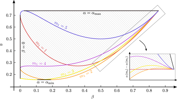
Figure 3: Demarcation lines of the allowed $\alpha\beta$-space (shaded area) for an $SU(7)$ invariant potential with a fundamental and an adjoint representation. The curved lines (in color) follow equation (39), while the straight ones (in black) are described by the expressions (43)–(45), obtained in reference [21]. The inlet clarifies what is happening on the right side of the plot, with the $m_{1}=1,2,3$ curves all being important for the demarcation of the bottom border line.

Since the shape of the $\alpha\beta$-space is quite elaborate, we may focus instead on the rectangle containing it and derive the following simple but potentially useful BFB condition — which is sufficient but not necessary for vacuum stability. It consists on demanding that all the following expressions are positive:

$$\lambda_{\phi},\;\lambda_{\Delta}+\alpha_{\textrm{min}/\textrm{max}}\lambda_{\Delta}^{\prime},\;\lambda_{\phi\Delta}+\beta_{\textrm{min}/\textrm{max}}\lambda_{\phi\Delta}^{\prime}+\sqrt{\lambda_{\phi}\left(\lambda_{\Delta}+\alpha_{\textrm{min}/\textrm{max}}\lambda_{\Delta}^{\prime}\right)}\,.$$ (46)

One should take every combination of $\alpha$ and $\beta$ at their minimum and maximum values (see equations (41), (42) and the text immediately preceding them), hence there is a total of $1+2+4=7$ quantities to be checked.

6 The 1-2-3 $SU(2)$ potential

Neutrino masses can be generated at tree level by introducing in the Standard Model a scalar $\Delta$ with the $SU(2)_{L}\times U(1)_{Y}$ quantum numbers $\left(\boldsymbol{3},1\right)$. Via the seesaw type-II mechanism, neutrinos acquire a mass $m_{\nu}=Y_{\nu}\mu\left\langle\phi\right\rangle^{2}/m_{\Delta^{0}}^{2}$ where

• $Y_{\nu}$ is the Yukawa coupling matrix regulating the interaction $L_{i}^{T}CL_{j}\Delta$ between left-handed leptons and $\Delta$;

• $m_{\Delta^{0}}$ stands for the mass of the neutral component of $\Delta$;

• $\mu$ is a mass which controls the strength of the trillinear interaction $\phi^{\dagger}\Delta\phi^{*}$ between $\Delta$ and the Higgs doublet $\phi$.

Note that lepton number is restored in the limit where $\mu$ vanishes, so this symmetry protects $\mu$ from big radiative corrections, and that is why the smallness of $m_{\nu}$ is usually attributed to the tiny value of this mass parameter.

As an alternative, lepton number might be spontaneously violated. To that end one can introduce a scalar singlet with no hypercharge and two units of lepton number [12], so that an interaction $\frac{\lambda_{\sigma\phi\Delta}}{2}\sigma\phi^{\dagger}\Delta\phi^{*}+\textrm{h.c.}$ is allowed by all symmetries; once this scalar acquires a vacuum expectation value, an effective $\mu$ equal to $\lambda_{\sigma\phi\Delta}\left\langle\sigma\right\rangle$ is generated (see figure 4).

Figure 4: Neutrino mass diagram in the 1-2-3 model. When $\sigma$ acquires a non-zero vacuum expectation value, the $LL\phi\phi$ Weinberg operator [23] is generated ($L$ and $\phi$ represent the left-handed leptons and the Higgs doublet).

With a singlet $\sigma$ ($\boldsymbol{1}$), a doublet $\phi$ ($\boldsymbol{2}$) and a triplet $\Delta$ ($\boldsymbol{3}$), this setup is sometimes called the 1-2-3 model. The full scalar potential reads

$$V^{(4)}\left(\phi,\Delta,\sigma\right) =V^{(4)}\left(\phi,\Delta\right)+\frac{\lambda_{\sigma}}{2}\left|\sigma\right|^{4}+\lambda_{\sigma\phi}\left|\sigma\right|^{2}\phi^{\dagger}\phi+\lambda_{\sigma\Delta}\left|\sigma\right|^{2}\textrm{Tr}\left(\Delta\Delta^{*}\right)+\left(\frac{\lambda_{\sigma\phi\Delta}}{2}\sigma\phi^{\dagger}\Delta\phi^{*}+\textrm{h.c.}\right)$$ (47)

where $V^{(4)}\left(\phi,\Delta\right)$ contains only terms with $\phi$ and $\Delta$ and was given previously in equation (3). Once again a gauge transformation can be used to diagonalize $\Delta$ ($\rightarrow\textrm{diag}\left(\Delta_{1},\Delta_{2}\right)$), in which case we may make the replacements $\phi^{\dagger}\phi\rightarrow\left|\phi_{1}\right|^{2}+\left|\phi_{2}\right|^{2}$, $\textrm{Tr}\left(\Delta\Delta^{*}\right)\rightarrow\left|\Delta_{1}\right|^{2}+\left|\Delta_{2}\right|^{2}$ and $\phi^{\dagger}\Delta\phi^{*}\rightarrow\left(\phi_{1}^{*}\right)^{2}\Delta_{1}+\left(\phi_{2}^{*}\right)^{2}\Delta_{2}$. This last expression is the only one sensitive to the phases of the fields, so the potential above is minimal when

$$\frac{\lambda_{\sigma\phi\Delta}}{2}\sigma\phi^{\dagger}\Delta\phi^{*}+\textrm{h.c.}=-\left|\lambda_{\sigma\phi\Delta}\right|\left|\sigma\right|\left(\left|\phi_{1}\right|^{2}\left|\Delta_{1}\right|+\left|\phi_{2}\right|^{2}\left|\Delta_{2}\right|\right)\,.$$ (48)

We have seen that $V^{(4)}\left(\phi,\Delta\right)$ depends only on 4 field components — $\left|\phi_{1,2}\right|$ and $\left|\Delta_{1,2}\right|$ — or equivalently $\left|\phi_{1}\right|^{2}+\left|\phi_{2}\right|^{2}$, $\left|\Delta_{1}\right|^{2}+\left|\Delta_{2}\right|^{2}$, $\alpha$ and $\beta$ (see equation (8)). With the introduction of $\sigma$, the minimum of the potential will depend only on one extra field $\left|\sigma\right|$, nevertheless the potential itself becomes significantly more complicated, with 4 new $\lambda$’s. In fact, to find the BFB conditions of the 1-2-3 potential it would be necessary to minimize a polynomial with a quadratic dependence on the $\left|\phi_{i}\right|^{2}$ and crucially a quartic dependence on the variables $\left|\sigma\right|$ and $\left|\Delta_{i}\right|$. The results on the copositivity of quadratic functions cannot be used here, and one can appreciate from [24, 9] that handling multi-variable quartic functions is very complicated, hence it seems unwise to try to find the necessary and sufficient BFB of the potential in equation (47). However, for the study of neutrino masses in the 1-2-3 model it might be good enough to find some acceptable values of the $\lambda$’s (not necessarily all of them).

One important case is when the coupling $\lambda_{\sigma\phi\Delta}$ is too small to be relevant for the stability of the vacuum. The neutrino mass matrix is given by the formula $Y_{\nu}\lambda_{\sigma\phi\Delta}^{*}\left\langle\sigma\right\rangle\left\langle\phi\right\rangle^{2}/m_{\Delta^{0}}^{2}$ with $m_{\Delta^{0}}$ often taken to be quite low — of the TeV order — so the product $Y_{\nu}\lambda_{\sigma\phi\Delta}^{*}\left\langle\sigma\right\rangle$ must be tiny. Therefore the approximation $\lambda_{\sigma\phi\Delta}\approx 0$ is an important and well motivated one. Without this coupling, the 1-2-3 potential becomes a quadratic function of the non-negative variables $\left|\phi_{1,2}\right|^{2}$, $\left|\Delta_{1,2}\right|^{2}$ and $\left|\sigma\right|^{2}$, hence the potential is bounded from below if and only if the symmetric matrix

$$\left(\begin{array}[]{ccccc}\lambda_{\phi}&\lambda_{\phi}&\lambda_{\phi\Delta}+\lambda_{\phi\Delta}^{\prime}&\lambda_{\phi\Delta}&\lambda_{\sigma\phi}\\ \cdot&\lambda_{\phi}&\lambda_{\phi\Delta}&\lambda_{\phi\Delta}+\lambda_{\phi\Delta}^{\prime}&\lambda_{\sigma\phi}\\ \cdot&\text{$\cdot$}&\lambda_{\Delta}+\lambda_{\Delta}^{\prime}&\lambda_{\Delta}&\lambda_{\sigma\Delta}\\ \cdot&\cdot&\cdot&\lambda_{\Delta}+\lambda_{\Delta}^{\prime}&\lambda_{\sigma\Delta}\\ \text{$\cdot$}&\cdot&\cdot&\cdot&\lambda_{\sigma}\end{array}\right)$$ (49)

is co-positive. It is straightforward to obtain the explicit set of inequalities which the $\lambda$’s must obey (for example with the method described in [25]; see also [8]), however I will not reproduce the expressions here since they are long and not very instructive.

If $\left|\lambda_{\sigma\phi\Delta}\right|$ is sizable one might consider the following strategy. For any scalar field configuration, it is either true that $\left|\sigma\right|\geq\sqrt{\left|\Delta_{1}\right|^{2}+\left|\Delta_{2}\right|^{2}}$ or the opposite, hence

$$-\left|\sigma\right|\left(\left|\phi_{1}\right|^{2}\left|\Delta_{1}\right|+\left|\phi_{2}\right|^{2}\left|\Delta_{2}\right|\right)\leq-\left|\sigma\right|^{2}\left(\left|\phi_{1}\right|^{2}+\left|\phi_{2}\right|^{2}\right)\textrm{ or }-\left(\left|\Delta_{1}\right|^{2}+\left|\Delta_{2}\right|^{2}\right)\left(\left|\phi_{1}\right|^{2}+\left|\phi_{2}\right|^{2}\right)$$ (50)

By replacing in the potential $V^{(4)}\left(\phi,\Delta,\sigma\right)$ the left term with the terms on the right, we get two potentials, both of which depend only on $\left|\phi_{1,2}\right|^{2}$, $\left|\Delta_{1,2}\right|^{2}$ and $\left|\sigma\right|^{2}$. Therefore the 1-2-3 potential is bounded from below if both the following symmetric matrices are co-positive:

$$\left(\begin{array}[]{ccccc}\lambda_{\phi}&\lambda_{\phi}&\lambda_{\phi\Delta}+\lambda_{\phi\Delta}^{\prime}&\lambda_{\phi\Delta}&\lambda_{\sigma\phi}-\left|\lambda_{\sigma\phi\Delta}\right|\\ \cdot&\lambda_{\phi}&\lambda_{\phi\Delta}&\lambda_{\phi\Delta}+\lambda_{\phi\Delta}^{\prime}&\lambda_{\sigma\phi}-\left|\lambda_{\sigma\phi\Delta}\right|\\ \cdot&\text{$\cdot$}&\lambda_{\Delta}+\lambda_{\Delta}^{\prime}&\lambda_{\Delta}&\lambda_{\sigma\Delta}\\ \cdot&\cdot&\cdot&\lambda_{\Delta}+\lambda_{\Delta}^{\prime}&\lambda_{\sigma\Delta}\\ \text{$\cdot$}&\cdot&\cdot&\cdot&\lambda_{\sigma}\end{array}\right)\,,$$ (56)

$$\left(\begin{array}[]{ccccc}\lambda_{\phi}&\lambda_{\phi}&\lambda_{\phi\Delta}+\lambda_{\phi\Delta}^{\prime}-\left|\lambda_{\sigma\phi\Delta}\right|&\lambda_{\phi\Delta}-\left|\lambda_{\sigma\phi\Delta}\right|&\lambda_{\sigma\phi}\\ \cdot&\lambda_{\phi}&\lambda_{\phi\Delta}-\left|\lambda_{\sigma\phi\Delta}\right|&\lambda_{\phi\Delta}+\lambda_{\phi\Delta}^{\prime}-\left|\lambda_{\sigma\phi\Delta}\right|&\lambda_{\sigma\phi}\\ \cdot&\text{$\cdot$}&\lambda_{\Delta}+\lambda_{\Delta}^{\prime}&\lambda_{\Delta}&\lambda_{\sigma\Delta}\\ \cdot&\cdot&\cdot&\lambda_{\Delta}+\lambda_{\Delta}^{\prime}&\lambda_{\sigma\Delta}\\ \text{$\cdot$}&\cdot&\cdot&\cdot&\lambda_{\sigma}\end{array}\right)\,.$$ (62)

Note however that this is not a necessary condition: the 1-2-3 potential might be bounded from below even if it fails to pass this test.

7 Conclusions

Scalar potentials are quartic functions of several field components, hence their analysis can be quite complicated. That is why it is only possible to write down the necessary and sufficient conditions for these functions to be bounded from below in simple cases, when the number of scalar representations is small. In this work, I have derived these constraints for $SU(n)$ invariants potentials with two fields: one transforming under the fundamental representation and the other as a 2-index representation (the symmetric or the anti-symmetric one). The case where the 2-index representation is the adjoint is substantially more complicated, hence I have only provided in a closed form a sufficient condition for the potential to be stable.

The combination of fields above mentioned appears in several models extending the Standard Model gauge group. The special case where $n=2$ and the scalars are a doublet and a triplet is particularly important because these fields participate in the seesaw type-II mechanism which might be responsible for neutrino mass generation. The BFB conditions for this scenario were already presented in [3], although a crucial step necessary to derive this result was not shown explicitly, as the relevant calculations were performed with a computer algebra system. In this work, I have provided a fully analytical proof of this result, which is valid for any $SU(n)$ group.

One can also add a scalar singlet to the Standard Model on top of the triplet used in the type-II seesaw mechanism. With the introduction of the singlet, lepton number can be broken spontaneously rather than explicitly, leading to important phenomenological consequences. Yet the scalar potential of this so-called 1-2-3 model contains nine quartic couplings, making it hard to derive necessary and sufficient BFB conditions in full generality. Therefore I considered the physically well motivated approximation where one of the interactions is negligible, in which case one can use well known results on the co-positivity of matrices to derive the relevant conditions. For those cases where all quartic couplings are relevant, I also derived a sufficient (but not necessary) condition which can be used to pick acceptable coupling constants.

Appendix

As discussed in the main text, the $2n$ vectors in equations (17) and (18) can be used to identify the allowed values of the $\alpha$ and $\beta$ variables defined in expression (8). In particular, at the border of the valid $\alpha\beta$-region, these vectors must either be null or point in a single direction. By carefully considering the right-hand side of the expressions (17) and (18), one of the following possibilities must be true.

1. For all $i$ such that $x_{i}\neq 0$ (there must be at least one such case since $\sum_{i}x_{i}=1$) we have $y_{i}=\beta$. We can further divide this possibility in three cases.

   1. $\beta=0$. This means that $x_{i}\neq 0$ implies $y_{i}=0$. So we can have at most $n-1$ non-zero $y_{i}$ which in turn means that $\alpha\in\left[1/(n-1),1\right]$.

   2. $\beta=\alpha\neq 0$. In this scenario, the vectors (17) and (18) are aligned only if the value of all non-zero $x_{i}$ or all non-zero $y_{i}$ is $\beta$($=\alpha$). So we conclude that $\alpha=\beta=1/m$ where $m$ is the number of $x_{i}$ or $y_{i}\neq 0$.

   3. $\beta\neq 0,\alpha$. This is undoubtedly the most important case. By assumption, if $x_{i}\neq 0$ then $y_{i}=\beta$, and for all such cases the vectors $\left(2\left(\beta-\alpha\right),x_{i}-\beta\right)^{T}$ are proportional to each other only if the $x_{i}$ take a constant value. In other words, there are $m$ non-zero $x_{i}$ and they all have the same value $1/m$ (because $\sum_{i}x_{i}=1$), plus the corresponding $y_{i}$ are equal to $\beta$. Any additional non-zero$y_{i}$ must be paired with a null $x_{i}$, and in all such cases the alignment of the vectors $\left(2\left(y_{i}-\alpha\right),\beta\right)^{T}$ and $\left(2\left(\beta-\alpha\right),1/m-\beta\right)^{T}$ requires that those $y_{i}$ also have a constant value given by the expression $y_{i}=\left(m\beta^{2}-\alpha\right)/\left(m\beta-1\right)\equiv\omega$. Let us assume that there are $m^{\prime}$ such occurrences; the overall picture is this: there are $m$ cases $\left(x_{i},y_{i}\right)=\left(1/m,\beta\right)$, $m^{\prime}$ occurrences of $\left(x_{i},y_{i}\right)=\left(0,\omega\right)$ and all other $\left(x_{i},y_{i}\right)$ are equal to $\left(0,0\right)$. From the relation $1=\sum_{i}y_{i}=m\beta+m^{\prime}\omega$ we conclude that

      $$\alpha=\frac{1-2m\beta+\left(m^{2}+mm^{\prime}\right)\beta^{2}}{m^{\prime}}\,.$$ (63)

      The non-negative integers $m$ and $m^{\prime}$ can take any values as long as $m\geq 1$ and $m+m^{\prime}\leq n$. However, note that the case $m=1$ and $m^{\prime}=n-1$ leads to the smallest value of $\alpha$ (for any fixed $\beta$). This important setup corresponds to the quadratic dependence of $\alpha$ on $\beta$ shown in equation (19) which defines a line of utmost importance for the extraction of the boundedness from below condition of the scalar potential given in (3).

2. There is at least one $i$ such that $x_{i}\neq 0$ and the corresponding $y_{i}\neq\beta$. If this is the case, then all $y_{i}$ must either be $0$ or $\alpha$ in order for the vectors $y_{i}\left(y_{i}-\alpha,x_{i}-\beta\right)^{T}$ to be collinear with $\left(0,1\right)^{T}$. If we were to call $m$ to the number of $y_{i}$ different from zero (this must be an integer between 1 and $n-1$), then we conclude from $\sum_{i}y_{i}=1$ that $\alpha=1/m$. The $x_{i}$ are unconstrained in this scenario, so it follows that $\beta$ can be anywhere in the range $\left[0,\alpha\right]$ (the value $\beta=0$ is reached for example when a single $x_{i}=1$ is paired with a null $y_{i}$; on the other hand when all null $y_{i}$ have an associated $x_{i}=0$ then $\beta=\alpha$).

The four cases above (1.a, 1.b, 1.c and 2) correspond only to potential fragments of the border of the $\alpha\beta$-region. In fact, some of them are in the interior of this space. Figure 1 depicts the actual border: the vertical line with $\beta=0$ and $\alpha\in\left[1/(n-1),1\right]$ (case 1.a), the horizontal line $\alpha=1$ and $\beta\in\left[0,1\right]$ (case 2 with $m=1$) and the parabola (19) with $\beta\in\left[0,1\right]$ (case 1.c).

Note that for a fixed value of $\alpha$, if we manage to find two valid values of $\beta$ then all values in between them are equally achievable. Using this fact, we conclude that all the space inside the border (shaded area in figure 1) is allowed as well.