\jyear

2022

[1,2]\fnmDavid \surRügamer

[1]\orgdivDepartment of Statistics, \orgnameLMU Munich, \orgaddress\cityMunich, \countryGermany

2]\orgdivInstitute of Statistics, \orgnameRWTH Aachen, \orgaddress\cityAachen, \countryGermany

3]\orgdivKOF Swiss Economic Institute, \orgnameETH Zurich, \orgaddress\cityZurich, \countrySwitzerland

4]\orgdivChair of Statistics, \orgnameUniversity of Goettingen, \orgaddress\cityGoettingen, \countryGermany

5]\orgdivEpidemiology, Biostatistics and Prevention Institute, \orgnameUniversity of Zurich, \orgaddress\cityZurich, \countrySwitzerland

Probabilistic Time Series Forecasts with Autoregressive Transformation Models

david@stat.uni-muenchen.de    \fnmPhilipp F.M. \surBaumann baumann@kof.ethz.ch    \fnmThomas \surKneib tkneib@uni-goettingen.de    \fnmTorsten \surHothorn torsten.hothorn@uzh.ch * [ [ [ [
Abstract

Probabilistic forecasting of time series is an important matter in many applications and research fields. In order to draw conclusions from a probabilistic forecast, we must ensure that the model class used to approximate the true forecasting distribution is expressive enough. Yet, characteristics of the model itself, such as its uncertainty or its feature-outcome relationship are not of lesser importance. This paper proposes Autoregressive Transformation Models (ATMs), a model class inspired by various research directions to unite expressive distributional forecasts using a semi-parametric distribution assumption with an interpretable model specification. We demonstrate the properties of ATMs both theoretically and through empirical evaluation on several simulated and real-world forecasting datasets.

keywords:
Semi-parametric Models, Conditional Density Estimation, Distributional Regression, Normalizing Flows

1 Introduction

Conditional models describe the conditional distribution $F_{Y\mid x}(y\mid\bm{x})$ of an outcome $Y$ conditional on observed features $\bm{x}$ (see, e.g., Jordan et al, 2002). Instead of modeling the complete distribution of $Y\mid\bm{x}$, many approaches focus on modeling a single characteristic of this conditional distribution. Predictive models, for example, often focus on predicting the average outcome value, i.e., the expectation of the conditional distribution. Quantile regression (Koenker, 2005), which is used to model specific quantiles of $Y\mid\bm{x}$, is more flexible in explaining the conditional distribution by allowing (at least theoretically) for arbitrary distribution quantiles. Various other approaches allow for an even richer explanation by, e.g., directly modeling the distribution’s density $f_{Y\mid\bm{x}}$ and thus the whole distribution $F_{Y\mid x}(y\mid\bm{x})$. Examples include mixture density networks (Bishop, 1994) in machine learning, or, in general, probabilistic modeling approaches such as Gaussian processes or graphical models (Murphy, 2012). In statistics and econometrics, similar approaches exist, which can be broadly characterized as distributional regression (DR) approaches (Chernozhukov et al, 2013; Foresi and Peracchi, 1995; Rügamer et al, 2020; Wu and Tian, 2013). Many of these approaches can also be regarded as conditional density estimation (CDE) models.

Modeling $F_{Y\mid x}(y\mid\bm{x})$ is a challenging task that requires balancing the representational capacity of the model (the expressiveness of the modeled distribution) and its risk for overfitting. While the inductive bias introduced by parametric methods can help to reduce the risk of overfitting and is a basic foundation of many autoregressive models, their expressiveness is potentially limited by this distribution assumption (cf. Figure 1).

Refer to caption
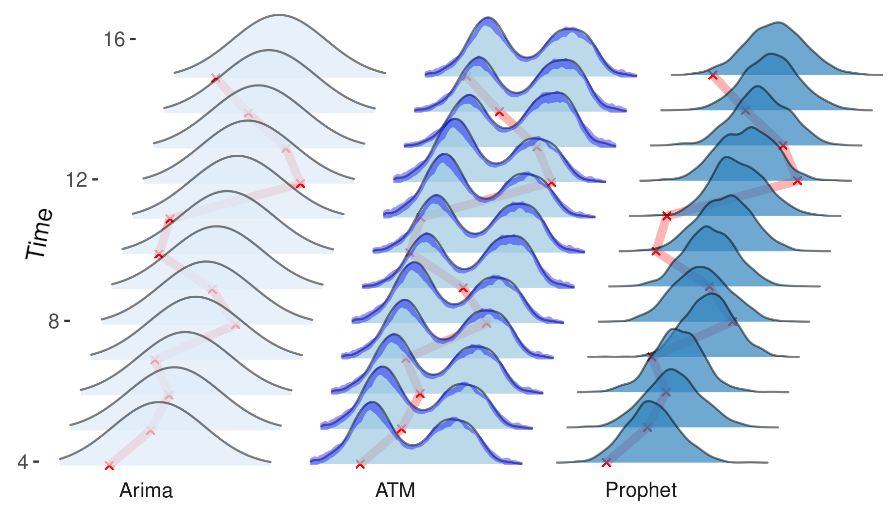
Figure 1: Exemplary comparison of probabilistic forecasting approaches with the proposed method (ATM; with its uncertainty depicted by the darker shaded area) for a given time series (red line). While other methods are not expressive enough and tailored toward a simple unimodal distribution, our approach allows for complex probabilistic forecasts (here a bimodal distribution where the inducing mixture variable is unknown to all methods).
Our contributions

In this work, we propose a new and general class of semi-parametric autoregressive models for time series analysis called autoregressive transformation models (ATMs; Section 3) that learn expressive distributions based on interpretable parametric transformations. ATMs can be seen as a generalization of autoregressive models. We study the autoregressive transformation of order $p$ (AT($p$)) in Section 4 as the closest neighbor to a parametric autoregressive model, and derive asymptotic results for estimated parameters in Section 4.2. Finally, we provide evidence for the efficacy of our proposal both with numerical experiments based on simulated data and by comparing ATMs against other existing time series methods.

2 Background and Related Work

Approaches that model the conditional density can be distinguished by their underlying distribution assumption. Approaches can be parametric, such as mixture density networks (Bishop, 1994) for conditional density estimation and then learn the parameters of a pre-specified parametric distribution or non-parametric such as Bayesian non-parametrics (Dunson, 2010). A third line of research that we describe as semi-parametric, are approaches that start with a simple parametric distribution assumption $F_{Z}$ and end up with a far more flexible distribution $F_{Y\mid\bm{x}}$ by transforming $F_{Z}$ (multiple times). Such approaches have sparked great interest in recent years, triggered by research ideas such as density estimation using non-linear independent components estimation or real-valued non-volume preserving transformations (Dinh et al, 2017). A general notion of such transformations is known as normalizing flow (NF; Papamakarios et al, 2021), where realizations $\bm{z}\sim F_{Z}$ of an error distribution $F_{z}$ are transformed to observations $\bm{y}$ via

$\displaystyle\bm{y}$ $\displaystyle=h_{k}\circ h_{k-1}\circ\cdots\circ h_{1}(\bm{z})$ (1)

using $k$ transformation functions. Many different approaches exist to define expressive flows. These are often defined as a chain of several transformations or an expressive neural network and allow for universal representation of $F_{Y\mid\bm{x}}$ (Papamakarios et al, 2021). Autoregressive models (e.g., Bengio and Bengio, 1999; Uria et al, 2016) for distribution estimation of continuous variables are a special case of NFs, more precisely autoregressive flows (AFs; Kingma et al, 2016; Papamakarios et al, 2017), with a single transformation.

Transformation models

Transformation models (TMs; Hothorn et al, 2014), a similar concept to NFs, only consist of a single transformation and thereby better allow theoretically studying model properties. The transformation in TMs is chosen to be expressive enough on its own and comes with desirable approximation guarantees. Instead of a transformation from $\bm{z}$ to $\bm{y}$, TMs define an inverse flow $h(\bm{y})=\bm{z}$. The key idea of TMs is that many well-known statistical regression models can be represented by a base distribution $F_{Z}$ and some transformation function $h$. Prominent examples include linear regression or the Cox proportional hazards model (Cox, 1972), which can both be seen as a special case of TMs (Hothorn et al, 2014). Various authors have noted the connection between autoregressive models and NFs (e.g., Papamakarios et al, 2021) and between TMs and NFs (e.g., Sick et al, 2021). Advantages of TMs and conditional TMs (CTMs) are their parsimony in terms of parameters, interpretability of the input-output relationship, and existing theoretical results (Hothorn et al, 2018). While mostly discussed in the statistical literature, various recent TM advancements have been also proposed in the field of machine learning (see, e.g., Van Belle et al, 2011) and deep learning (see, e.g., Baumann et al, 2021; Kook et al, 2021, 2022).

Time series forecasting

In time series forecasting, many approaches rely on autoregressive models, with one of the most commonly known linear models being autoregressive (integrated) moving average (AR(I)MA) models (see, e.g., Shumway et al, 2000). Extensions include the bilinear model of Granger and Andersen (1978); Rao (1981), or the Markov switching autoregressive model by Hamilton (2010). Related to these autoregressive models are stochastic volatility models (Kastner et al, 2017) building upon the theory of stochastic processes. In probabilistic forecasting, Bayesian model averaging (Raftery et al, 2005) and distributional regression forecasting (Schlosser et al, 2019) are two further popular approaches while many other Bayesian and non-Bayesian techniques exist (see, e.g., Gneiting and Katzfuss, 2014, for an overview).

2.1 Transformation models

Parametrized transformation models as proposed by Hothorn et al (2014, 2018) are likelihood-based approaches to estimate the CDF $F_{Y}$ of $Y$. The main ingredient of TMs is a monotonic transformation function $h$ to convert a simple base distribution $F_{Z}$ to a more complex and appropriate CDF $F_{Y}$. Conditional TMs (CTMs) work analogously for the conditional distribution of $Y$ given features $\bm{x}\in\chi$ from feature space $\chi$:

$$F_{Y\mid\bm{x}}(y)=\mathbb{P}(Y\leq y\mid\bm{x})=F_{Z}(h(y\mid\bm{x})).$$ (2)

CTMs learn $h(y\mid\bm{x})$ from the data, i.e., estimate a model for the (conditional) aleatoric uncertainty. A convenient parameterization of $h$ for continuous $Y$ are Bernstein polynomials (BSPs; Farouki, 2012) with order $M$ (usually $M\ll 50$). BSPs are motived by the Bernstein approximation (Bernstein, 1912) with uniform convergence guarantees for $M\to\infty$, while also being computationally attractive with only $M+1$ parameters. BSPs further have easy and analytically accessible derivatives, which makes them a particularly interesting choice for the change of random variables. We denote the BSP basis by $\bm{a}_{M}:\Xi\mapsto\mathbb{R}^{M+1}$ with sample space $\Xi$. The transformation $h$ is then defined as $h(y\mid\bm{x})=\bm{a}_{M}(y)^{\top}\bm{\vartheta}(\bm{x})$ with feature-dependent basis coefficients $\bm{\vartheta}$. This can be seen as an evaluation of $y$ based on a mixture of Beta densities $f_{Be(\kappa,\mu)}$ with different distribution parameters $\kappa,\mu$ and weights $\bm{\vartheta}(\bm{x})$:

$$\bm{a}_{M}(y)^{\top}\bm{\vartheta}(\bm{x})=\frac{\sum_{m=0}^{M}\vartheta_{m}(\bm{x})f_{Be(m+1,M-m+1)}(\tilde{y})}{M+1},$$ (3)

where $\tilde{y}$ is a rescaled version of $y$ to ensure $\tilde{y}\in[0,1]$. Restricting $\vartheta_{m}>\vartheta_{m-1}$ for $m=1,\ldots,M+1$ guarantees monotonicity of $h$ and thus of the estimated CDF. Roughly speaking, using BSPs of order $M$, allows to model the polynomials of degree $M$ of $y$.

2.2 Model definition

The transformation function $h$ can include different data dependencies. One common choice (Hothorn, 2020; Baumann et al, 2021) is to split the transformation function into two parts

$$h(y\mid\bm{x})=h_{1}(y,\bm{x})+h_{2}(\bm{x})=\bm{a}(y)^{\top}\bm{\vartheta}(\bm{x})+\beta(\bm{x}),$$ (4)

where $\bm{a}(y)$ is a pre-defined basis function such as the BSP basis (omitting $M$ for readability in the following), $\bm{\vartheta}:\chi_{\vartheta}\mapsto\mathbb{R}^{M+1}$ a conditional parameter function defined on $\chi_{\vartheta}\subseteq\chi$ and $\beta(\bm{x})$ models a feature-induced shift in the transformation function. The flexibility and interpretability of TMs stems from the parameterization

$$\bm{\vartheta}(\bm{x})=\sum_{j=1}^{J}\bm{\Gamma}_{j}.\bm{b}_{j}(\bm{x}),$$ (5)

where the matrix $\bm{\Gamma}_{j}\in\mathbb{R}^{(M+1)\times O_{j}},O_{j}\geq 1,$ subsumes all trainable parameters and represents the effect of the interaction between the basis functions in $\bm{a}$ and the chosen predictor terms $\bm{b}_{j}:\chi_{b_{j}}\mapsto\mathbb{R}^{O_{j}},\chi_{b_{j}}\subseteq\chi$. The predictor terms $\bm{b}_{j}$ have a role similar to base learners in boosting and represent simple learnable functions. For example, a predictor term can be the $j$th feature, $\bm{b}_{j}(\bm{x})=x_{j}$, and $\bm{\Gamma}_{j}\in\mathbb{R}^{(M+1)\times 1}$ describes the linear effect of this feature on the $M+1$ basis coefficients, i.e., how the feature $x_{j}$ relates to the density transformation from $Z$ to $Y\mid\bm{x}$. Other structured non-linear terms such as splines allow for interpretable lower-dimensional non-linear relationships. Various authors also proposed neural network (unstructured) predictors to allow potentially multidimensional feature effects or to incorporate unstructured data sources (Sick et al, 2021; Baumann et al, 2021; Kook et al, 2021). In a similar fashion, $\beta(\bm{x})$ can be defined using various structured and unstructured predictors.

Interpretability

Relating features and their effect in an additive fashion allows to directly assess the impact of each feature on the transformation and also whether changes in the feature just shift the distribution in its location or if the relationship also transforms other distribution characteristics such as variability or skewness (see, e.g., Baumann et al, 2021, for more details).

Relationship with autoregressive flows

In the notation of AFs, $h^{-1}(\cdot)$ is known as transformer, a parameterized and bijective function. By the definition of (4), the transformer in the case of TMs is represented by the basis function $\bm{a}(\cdot)$ and parameters $\bm{\vartheta}$. In AFs, these transformer parameters are learned by a conditioner, which in the case of TMs are the functions $\bm{b}_{j}$. In line with the assumptions made for AFs, these conditioners in TMs do not need to be bijective functions themselves.

3 Autoregressive Transformations

Inspired by TMs and AFs, we propose autoregressive transformation models (ATMs). Our work is the first to adapt TMs for time series data and thereby lays the foundation for future extensions of TMs for time series forecasting. The basic idea is to use a parameter-free base distribution $F_{Z}$ and transform this distribution in an interpretable fashion to obtain $F_{Y\mid\bm{x}}$. One of the assumptions of TMs is the stochastic independence of observations, i.e., $Y_{i}\mid\bm{x}_{i}\bot Y_{j}\mid\bm{x}_{j},i\neq j$. When $Y$ is a time series, this assumption does clearly not hold. In contrast, this assumption is not required for AFs.

Let $t\in\mathcal{T}\subseteq\mathbb{N}_{0}$ be a time index for the time series $(Y_{t})_{t\in\mathcal{T}}$. Assume

$$Y_{t}\mid\mathcal{F}_{t-1}\sim G(Y_{t-1},\ldots,Y_{t-p}\mathchar 24635\relax\;\bm{\theta})$$ (6)

for some $p\in\{1,\ldots,t\}$, distribution $G$, parameter $\bm{\theta}\in\Theta$ with compact parameter space $\Theta\subset\mathbb{R}^{v}$ and filtration $\mathcal{F}_{s}$, $s\in\mathcal{T}$, $s<t$, on the underlying probability space. Assume that the joint distribution of $Y_{t},Y_{t-1},\ldots,Y_{1}$ possesses the Markov property with order $p$, i.e., the joint distribution, expressed through its absolutely continuous density $f$, can be rewritten as product of its conditionals with $p$ lags:

$$f(y_{t},\ldots,y_{1}\mid\bm{x})=\prod_{s=p+1}^{t}f(y_{s}\mid y_{s-1},\ldots,y_{s-p},\bm{x}).$$ (7)

We use $\bm{x}$ to denote (potentially time-varying) features that are additional (exogenous) features. Their time-dependency is omitted for better readability here and in the following. Given this autoregressive structure, we propose a time-dependent transformation $h_{t}$ that extends (C)TMs to account for filtration and time-varying feature information. By modeling the conditional distribution of all time points in a flexible manner, ATMs provide an expressive way to account for aleatoric uncertainty in the data.

Definition 1.

Autoregressive Transformation Models Let $h_{t},t\in\mathcal{T}$, be a time-dependent monotonic transformation function and $F_{Z}$ the parameter-free base distribution as in Definition 1 in the Supplementary Material. We define autoregressive transformation models as follows:

$$\begin{split}\mathbb{P}(Y_{t}\leq y_{t}\mid\mathcal{F}_{t-1},\bm{x})&=F_{Y_{t}\mid\mathcal{F}_{t-1},\bm{x}}(y_{t})\\ &=F_{Z}(h_{t}(y_{t}\mid\mathcal{F}_{t-1},\bm{x})).\end{split}$$ (8)

This can be seen as the natural extension of (2) for time series data with autoregressive property and time-varying transformation function $h_{t}$. In other words, (8) says that after transforming $y_{t}$ with $h_{t}$, its conditional distribution follows the base distribution $F_{Z}$, or vice versa, a random variable $Z\sim F_{Z}$ can be transformed to follow the distribution $Y_{t}\mid\bm{x}$ using $h_{t}^{-1}$.

Relationship with autoregressive models and autoregressive flows

Autoregressive models (AMs; Bengio and Bengio, 1999) and AFs both rely on the factorization of the joint distribution into conditionals as in (7). Using the CDF of each conditional in (7) as transformer in an AF, we obtain the class of AMs (Papamakarios et al, 2021). AMs and ATMs are thus both (inverse) flows using a single transformation, but with different transformers and, as we will outline in Section 3.2, also with different conditioners.

3.1 Likelihood-based estimation

Based on (7), (8) and the change of variable theorem, the likelihood contribution of the $t$th observation $y_{t}$ in ATMs is given by

$$\begin{split}&f_{Y\mid x}(y_{t}\mid\mathcal{F}_{t-1},\bm{x})=\\ &f_{Z}(h_{t}(y_{t}\mid\mathcal{F}_{t-1},\bm{x}))\cdot\bigl{\lvert}\frac{\partial h_{t}(y_{t}\mid\mathcal{F}_{t-1},\bm{x})}{\partial y_{t}}\bigr{\rvert}\end{split}$$

and the full likelihood for $T$ observations thus by

$$\begin{split}&f_{Y\mid x}(Y_{T},\ldots,Y_{1}\mid\mathcal{Y}_{0},\bm{x})=\\ &\prod_{t=1}^{T}\left\{f_{Z}(h_{t}(y_{t}\mid\mathcal{F}_{t-1},\bm{x}))\cdot\bigl{\lvert}\frac{\partial h_{t}(y_{t}\mid\mathcal{F}_{t-1},\bm{x})}{\partial y_{t}}\bigr{\rvert}\right\},\end{split}$$ (9)

where $\mathcal{Y}_{0}=(y_{0},\ldots,y_{-p+1})$ are known finite starting values and $\mathcal{F}_{0}$ only contains these values. Based on (9), we define the loss of all model parameters $\bm{\theta}$ as negative log-likelihood $-\ell(\bm{\theta}):=-\log f_{Y\mid x}(Y_{T},\ldots,Y_{1}\mid\mathcal{Y}_{0},\bm{x})$ given by

$$\begin{split}-\sum_{t=1}^{T}\Bigl{\{}\log f_{Z}(h_{t}(y_{t}\mid\mathcal{F}_{t-1},\bm{x}))+\\ \log\bigl{|}\frac{\partial h_{t}(y_{t}\mid\mathcal{F}_{t-1},\bm{x})}{\partial y_{t}}\bigr{|}\Bigr{\}},\end{split}$$ (10)

and use (10) to train the model.

As for AFs, many special cases can be defined from the above definition and more concrete structural assumptions for $h_{t}$ make ATMs an interesting alternative to other methods in practice. We will elaborate on meaningful structural assumptions in the following.

3.2 Structural assumptions

Refer to caption
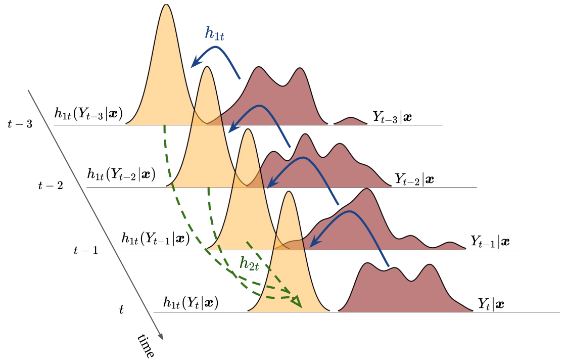
Figure 2: Illustration of a transformation process induced by the structural assumption of Section 3.2. The original data history $\mathcal{F}_{t-1}$ (red) is transformed into a base distribution (orange) using the transformation $h_{1t}$ (solid blue arrow) and then further transformed using $h_{2t}$ (dashed green arrow) to match the transformed distribution of the current time point $t$.

In CTMs, the transformation function $h$ is usually decomposed as $h(y\mid\bm{x})=h_{1}(y\mid\bm{x})+h_{2}(\bm{x})$, where $h_{1}$ is a function depending on $y$ and $h_{2}$ is a transformation-shift function depending only on $\bm{x}$. For time-varying transformations $h_{t}$ our fundamental idea is that the outcome $y_{t}$ shares the same transformation with its filtration $\mathcal{F}_{t-1}$, i.e., the lags $\mathcal{Y}_{t}=(y_{t-1},\ldots,y_{t-p})$. In other words, a transformation applied to the outcome must be equally applied to its predecessor in time to make sense of the autoregressive structural assumption. An appropriate transformation structure can thus be described by

$$\begin{split}h_{t}&(y_{t}\mid\mathcal{F}_{t-1},\bm{x})\\ &=h_{1t}(y_{t}\mid\bm{x})+h_{2t}((h_{1t}\odot\mathcal{Y}_{t}\mid\mathcal{F}_{t-1},\bm{x})\mid\bm{x})\\ &=:\lambda_{1t}+\lambda_{2t},\end{split}$$ (11)

for $t\in\mathcal{T}$, where $\odot$ indicates the element-wise application of $h_{1t}$ to all lags in $\mathcal{Y}_{t}$. In other words, ATMs first apply the same transformation $h_{1t}$ to $y_{t}$ and individually to $y_{t-1},y_{t-2},\ldots$, and then further consider a transformation function $h_{2t}$ to shift the distribution (and thereby potentially other distribution characteristics) based on the transformed filtration. While the additivity assumption of $\lambda_{1t}$ and $\lambda_{2t}$ seems restrictive at first glance, the imposed relationship between $y_{t}$ and $\mathcal{Y}_{t}$ only needs to hold in the transformed probability space. For example, $h_{1t}$ can compensate for a multiplicative autoregressive effect between the filtration and $y_{t}$ by implicitly learning a $\log$-transformation (cf. Section 5.1). At the same time, the additivity assumption offers a nice interpretation of the model, also depicted in Figure 2: After transforming $y_{t}$ and $\mathcal{Y}_{t}$, (11) implies that training an ATM is equal to a regression model of the form $\lambda_{1t}=\lambda_{2t}+\varepsilon$, with additive error term $\varepsilon\sim F_{Z}$ (cf. Proposition 1 in Supplementary Material A.2). This also helps explaining why only $\lambda_{2t}$ depends on $\mathcal{F}_{t-1}$: if $\lambda_{1t}$ also involves $\mathcal{F}_{t-1}$, ATMs would effectively model the joint distribution of the current time point and the whole filtration, which in turn contradicts the Markov assumption (7).

Specifying $h_{1t}$ very flexible clearly results in overfitting. As for CTMs, we use a feature-driven basis function representation $h_{1t}(y_{t}\mid\bm{x})=\bm{a}(y_{t})^{\top}\bm{\vartheta}(\bm{x})$ with BSPs $\bm{a}$ and specify their weights as in (5). The additional transformation $h_{2t}$ ensures enough flexibility for the relationship between the transformed response and the transformed filtration, e.g., by using a non-linear model or neural network. An interesting special case arises for linear transformations in $h_{2t}$, which we elaborate in Section 4 in more detail.

Interpretability

The three main properties that make ATMs interpretable are 1) their additive predictor structure as outlined in (5); 2) the clear relationship between features and the outcome through the BSP basis, and 3) ATM’s structural assumption as given in (11). As for (generalized) linear models, the additivity assumption in the predictor allows interpreting feature influences through their partial effect ceteris paribus. On the other hand, choices of $M$ and $F_{Z}$ will influence the relationship between features and outcome by inducing different types of models. A normal distribution assumption for $F_{Z}$ and $M=1$ will turn ATMs into an additive regression model with Gaussian error distribution (see also Section 4). For $M>1$, features in $h_{1}$ will also influence higher moments of $Y\mid\bm{x}$ and allow more flexibility in modeling $F_{Y\mid\bm{x}}$. For example, a (smooth) monotonously increasing feature effect will induce rising moments of $Y\mid\bm{x}$ with increasing feature values. Other choices for $F_{Z}$ such as the logistic distribution also allow for easy interpretation of feature effects (e.g., on the log-odds ratio scale; see Kook et al, 2021). Finally, the structural assumption of ATMs enforces that the two previous interpretability aspects are consistent over time. We will provide an additional illustrative example in Section 5.2, further explanations in Supplementary Material B, and refer to Hothorn et al (2014) for more details on interpretability of CTMs.

Implementation

In order to allow for a flexible choice of transformation functions and predictors $\bm{b}_{j}$, we propose to implement ATMs in a neural network and use stochastic gradient descent for optimization. While this allows for complex model definitions, there are also several computational advantages. In a network, weight sharing for $h_{1t}$ across time points is straightforward to implement and common optimization routines such as Adam (Kingma and Ba, 2014) prove to work well for ATMs despite the monotonicity constraints required for the BSP basis. Furthermore, as basis evaluations for a large number of outcome lags in $\mathcal{F}_{t-1}$ can be computationally expensive for large $p$ (with space complexity $\mathcal{O}(t\cdot M\cdot p)$) and add $M$ additional columns per lag to the feature matrix, an additional advantage is the dynamic nature of mini-batch training. In this specific case, it allows for evaluating the bases only during training and separately in each mini-batch. It is therefore never required to set up and store the respective matrices.

4 AT($p$) Model

A particular interesting special case of ATMs is the AT($p$) model. This model class is a direct extension of the well-known autoregressive model of order $p$ (short AR($p$) model; Shumway et al, 2000) to transformation models.

Definition 2.

AT($p$) model We define the AT($p$) model, a special class of ATMs, by setting $h_{1t}(y_{t}\mid\bm{x})=\bm{a}(y_{t})^{\top}\bm{\vartheta}(\bm{x})$, and $h_{2t}(\mathcal{F}_{t-1},\bm{x})=\sum_{j=1}^{p}\phi_{j}h_{1t}(y_{t-j})+r(\bm{x})$, i.e., an autoregressive shift term with optional exogenous remainder term $r(\bm{x})$.

As for classical time series approaches, $\phi_{j}$ are the regression coefficients relating the different lags to the outcome and $r$ is a structured model component (e.g., linear effects) of exogenous features that do not vary over time.

4.1 Model Details

The AT($p$) model is a very powerful and interesting model class for itself, as it allows to recover the classical time series AR($p$) model when setting $M=1$, $\bm{\vartheta}(\bm{x})\equiv\bm{\vartheta}$ and $r(\bm{x})\equiv 0$ (see Proposition 2 in Supplementary Material A for a proof of equivalence). But it can also be extended to more flexible autoregressive models in various directions. We can increase $M$ to get a more flexible density, allowing us to deviate from the base distribution assumption $F_{Z}$, e.g., to relax the normal distribution assumption of AR models. Alternatively, incorporating exogenous effects into $h_{1t}$ allows to estimate the density data-driven or to introduce exogenous shifts in time series using features $\bm{x}$ in $r(\bm{x})$. ATMs can also recover well-known transformed autoregressive models such as the multiplicative autoregressive model (Wong and Li, 2000) as demonstrated in Section 5.1. When specifying $M$ large enough, an AT($p$) model will, e.g., learn the log-transformation function required to transform a multiplicative autoregressive time series to an additive autoregressive time series on the log-scale. In general, this allows the user to learn autoregressive models without the need to find an appropriate transformation before applying the time series model. This means that the uncertainty about preprocessing steps (e.g., a Box-Cox transformation; Sakia, 1992) is incorporated into the model estimation, making parts of the pre-processing obsolete for the modeler and its uncertainty automatically available.

Non-linear extensions of AT($p$) models can be constructed by modeling $\mathcal{Y}_{t}$ in $h_{2t}$ non-linearly, allowing ATMs to resemble model classes such as non-linear AR models with exogenous terms (e.g., Lin et al, 1996). In practice, values for $p$ can, e.g., be found using a (forward) hyperparameter search by comparing the different model likelihoods.

4.2 Asymptotic theory

Refer to caption
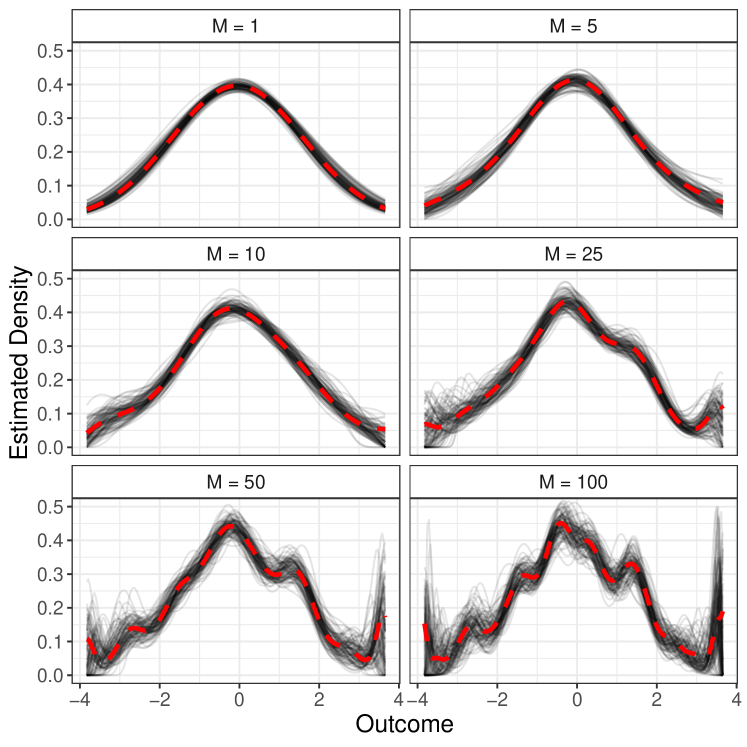
Figure 3: Aleatoric vs. epistemic uncertainty: Different plots correspond to different orders of the BSP basis $M$, inducing different amounts of expressiveness and aleatoric uncertainty. In each plot, the fitted density is shown in red, and model uncertainties of this density based on the epistemic uncertainty in black. Epistemic uncertainty is generated according to results in Theorem 2 and 3.

An important yet often neglected aspect of probabilistic forecasts is the epistemic uncertainty, i.e., the uncertainty in model parameters. Based on general asymptotic theory for time series models (Ling and McAleer, 2010), we derive theoretical properties for AT($p$)s in this section.

Let $\bm{\theta}^{\ast}$ be the true value of $\bm{\theta}$ and interior point of $\Theta$. We define the following quantities involved in standard asymptotic MLE theory: Let $\hat{\bm{\theta}}_{T}=\arg\min_{\Theta}-\ell(\bm{\theta})$ be the parameter estimator based on Maximum-Likelihood estimation (MLE), $\nabla_{T}(\bm{\theta})=\partial\ell_{T}(\bm{\theta})/\partial\bm{\theta}$, $\mathcal{J}_{T}(\bm{\theta})=-\partial^{2}\ell_{T}(\bm{\theta})/(\partial\bm{\theta}\partial\bm{\theta}^{\prime})$, $\mathcal{I}=\mathbb{E}_{G}(\mathcal{J}_{T}(\bm{\theta}^{\ast}))$ and $\mathfrak{J}=\mathbb{E}_{G}(\nabla_{T}(\bm{\theta}^{\ast})\nabla^{\top}_{T}(\bm{\theta}^{\ast}))$. We further state necessary assumptions to apply the theory of Ling and McAleer (2010) for a time series $(Y_{t})_{t\in\mathcal{T}}$ with known initial values $\mathcal{Y}_{0}$ as defined in Section 3.

Assumption 1.

Assume

  • (i)

    $(Y_{t})_{t\in\mathcal{T}}$ is strictly stationary and ergodic;

  • (ii)

    $\mathbb{E}_{G}\{\sup_{\bm{\theta}\in\Theta}[\ell_{T}(\bm{\theta})]\}<\infty$ and $\bm{\theta}^{\ast}$ is unique;

  • (iii)

    $\nabla_{T}(\bm{\theta}^{\ast})$ is a martingale difference w.r.t. $\mathcal{F}_{T-1}$ with $0<\mathfrak{J}<\infty$;

  • (iv)

    $\mathcal{I}$ is positive-definite and for some $\xi>0$ 𝔼G{sup𝜽:θ-θ^¡ξ  J_T(θ  } ¡ . Assumptions 1 are common assumptions required for many time series models. We require only these and no other assumptions since AT(p)s and non-linear extensions are fully-parameterized time series models. This allows us to derive general statistical inference theory for AT(p) models. 
    Theorem 1 (Consistency).

    If elements in Y0 are finite and Assumption 1(i) holds, then ^θTa.s.θ for T.

     As stated in Hothorn et al (2018), Assumption 1(ii) holds if 𝐚 is not arbitrarily ill-posed. In practice, both a finite 𝒴0 and Assumption 1(i) are realistic assumptions. Making two additional and also rather weak assumptions (1(iii)-(iv)) allows to derive the asymptotic normal distribution for 𝛉^
    Theorem 2 (Asymptotic Normality).

    If y0 is finite and Assumptions 1 hold, then for T,

    θ^_T = θ^+ O((loglogT) / T) and T(θ^_T - θ^DN(0, I^-1 J I^-1). Based on the same assumptions, a consistent estimator for the covariance can be derived. 
    Theorem 3 (Consistent Covariance Estimator).

    For finite y0 and under Assumptions 1,

    I^_T = 1T_t=1^T J_T(θ^_T) and J^_T = 1T_t=1^T _T(θ^_T) ^_T(θ^_T) are consistent estimators for  and 𝔍, respectively. The previous theorems can be proven by observing that the AT(p) model structure and all made assumptions follow the general asymptotic theory for time series models as given in Ling and McAleer (2010). See Supplementary Material A for details. Using the above results, we can derive statistically valid UQ. An example is depicted in Figure 3. Since h is parameterized through 𝜽, it is also possible to derive the so-called structural uncertainty of ATMs, i.e., the uncertainty induced by the discrepancy between the model’s CDF FYx(y𝒙;𝜽) and the true CDF FYx(y𝒙) (Liu et al, 2019). More specifically, h can be represented using a linear transformation of 𝜽h=𝚼𝜽, implying the (co-)variance 𝚼1𝔍(𝜽)1𝚼 for h^
    Practical application

    ATM define the distribution FYtF-t1,x via =FYF-t1,xFZht, where ht is parameterized by θ. In order to assess parameter uncertainty in the estimated density as, e.g. visualized in Figure 1 and 3, we propose to use a parametric Bootstrap described in detail in Supplementary Material C.

    5 Experiments

    Refer to caption
    Figure 4: Empirical evidence for the correctness of our theoretical results on PU: Expected vs. observed quantiles of the transformation function ht (left; one line per dataset) and model parameters θ for the different (lagged) transformed outcomes (right; one cross per dataset) based on 1000 simulation replications. The ideal angle bisector is plotted in red.

    We will first investigate theoretical properties of ATMs and the validity of statistical inference statements using simulation studies. We then compare our approach against other state-of-the-art methods described in the previous section on probabilistic forecasting tasks in a benchmark study. Additional results can be found in the Supplementary Material D.

    5.1 Simulation Study

    Table 1: Average and standard deviation (brackets) of the MSE (multiplied by 100 for better readability) between estimated and true coefficients in an AR(p) model using our approach on the tampered data (bottom row) and the corresponding oracle based on the true data (Oracle).
    T =p1 =p2 =p4
    Oracle 400 0.33 (0.31) 0.22 (0.19) 0.25 (0.13)
    AT(p) 0.52 (0.46) 0.33 (0.3) 0.34 (0.23)
    Oracle 800 0.27 (0.34) 0.13 (0.12) 0.13 (0.085)
    AT(p) 0.26 (0.36) 0.17 (0.17) 0.18 (0.12)
    Equivalence and consistency

    We first demonstrate Theorem 1 and Proposition 2 in the Supplementary Material, i.e., for growing number of observations AT(p) models can recover AR(p) models when equally specified. We therefore simulate various AR models using lags p{1,2,4}, T{200,400,800} and estimate both a classical AR(p) model and an AT(p) model for 20 replications. For the latter, we use the mapping derived in Proposition 2 to obtain the estimated AR coefficients from the AT(p) model. In Table D1 in the Supplementary Material D we compare both models based on their estimated coefficients against the ground truth using the mean squared error (MSE). Results show that the AT(p) model can empirically recover the AR(p) model very well.

    Flexibility

    Next, we demonstrate how the AT(p) model with =M30 can recover a multiplicative autoregressive process. We therefore generate data using an AR model with different lags p and observations n as before. This time, however, we provide the AT(p) model only with the exponentiated data =ˇytexp(yt). This means the model needs to learn the inverse transformation back to yt itself. Despite having to estimate the log-transformation in addition, the AT(p) model recovers the true model well and, for larger n, is even competitive to the ground truth model (Oracle) that has access to the original non-exponentiated data (cf. Table D2 for an excerpt of the results).

    Epistemic Uncertainty

    In this experiment we validate our theoretical results proposed in Section 4.2. As in the previous experiment, we try to learn the log-transformed AR model using an AT(=p3) model with coefficients (0.3,0.2,0.1). After estimation, we check the empirical distribution of ^θ and ^h against their respective theoretical one in 1000 simulation replications. Figure 4 depicts a quantile-quantile plot of the empirical and theoretical distribution for both h and all 4 parameters (intercept and three lag coefficients). The empirical distributions are well aligned with their theoretical distribution as derived in Section 4.2, confirming our theoretical results.

    5.2 Benchmarks

    Finally, we compare our approach to its closest neighbor in the class of additive models, the ARIMA model (Hyndman et al, 2021), against a simple Box-Cox transformation (BoxCox), a neural network for mean-variance estimation (MVN) and a mixture density network (MDN; Bishop, 1994). While there are many further forecasting techniques, especially in deep learning, we purposely exclude more complex machine and deep learning approaches to compare AT(p)s with approaches of similar complexity. More specifically, the different competitors were chosen to derive the following insights: The comparison of the AT(p) model with the ARIMA model will indicate whether relaxing the parametric assumption using TMs can improve performance while both methods take time series lags into account. The comparison of our method with BoxCox, on the other hand, will show similar performance if there is no relevant information in the lags of the time series. The MVN can potentially learn time series-specific variances but is not given the lagged information as input. A good performance of the MVN will thus indicate heteroscedasticity in the data generating process which can, however, be accounted for using a parametric distributional regression approach. Finally, the MDN is an alternative approach to the AT(p) model that tries to overcome the parametric assumption by modeling a mixture of normal distributions.

    Hyperparameter Setup

    We define the AT(p) model by using an unconditional ϑ parameter and use the lag structure as well as a time series identifier as a categorical effect in the additive predictor of β. We further investigate different number of BSPs M{5,10,30} and different number of lags p{1,2,3}. Model training for all models but the ARIMA model was done using 1000 epochs with early stopping and a batch size of 128. For the MDN, we define 3 mixtures and use the AT(p)’s β as an additive predictor for the mean of every mixture component. The MVN uses the time series identifier to learn individual means and variances. For ARIMA we used the auto.arima implementation (Hyndman et al, 2021) and performed a step-wise search via the AICc with different starting values for the order of the AR and the MA term. For the AR term, we consider the length of the corresponding forecasting horizon and halve this value. The search space for the MA term started either with 0 or 3. We chose the ARIMA model with the lowest AICc on the validation set. For the auto.arima model on the m4 data, we restrict the observations to be used for model selection to 242 in order to reduce the computational complexity. A larger number did not give higher logscores.

    Datasets

    We compare approaches on commonly used benchmark datasets electricity (elec; Yu et al, 2016), traffic forecasting (traffic; Yu et al, 2016), monthly tourism (Athanasopoulos et al, 2011), the hourly m4 dataset (Makridakis et al, 2018) and currency exchange (Lai et al, 2018). A short summary of these datasets can be found in Table D3 in the Supplementary Material.

    Evaluation

    For each proposed method and dataset, we report the log-scores (Gneiting et al, 2007) and average results across time series and time points. The datasets are split into a training, validation, and test set by adhering to their time ordering. Evaluation windows are defined as done in the reference given for every dataset.

    Table 2: Mean log-scores (higher is better) across 10 different initializations with standard deviations in brackets for each method (columns) and benchmark dataset (rows). Results for ARIMA are based on only one trial as there is typically no stochasticity in its results. The best performing method per data set is highlighted in bold.
    ARIMA AT(p) BoxCox MDN MVN
    elec -5.44 -5.35 (0.01) -8.37 (0.00) -5.20 (0.01) -9.51 (0.00)
    exchange 0.37 -3.50 (0.05) -0.69 (0.00) -4.02 (0.12) -0.70 (0.00)
    m4 -573.11 -6.72 (0.07) -10.7 (0.00) -6.75 (1.17) -12.0 (0.00)
    tourism -9.78 -9.38 (0.01) -11.5 (0.00) -77.8 (99.5) -12.7 (0.00)
    traffic 0.23 -1.09 (0.33) -0.03 (0.00) -1.06 (0.02) -0.25 (0.00)
    Results

    Table 2 shows the results of the comparison. Our approach always yields competitive and consistently good results while outperforming other models on most data sets.

    6 Conclusion and Outlook

    We have proposed ATMs, a flexible and comprehensible model class combining and extending various existing modeling approaches. ATMs allow for expressive probabilistic forecasts using a base distribution and a single transformation modeled by Bernstein polynomials. Additionally, a parametric inference paradigm based on MLE allows for statistical inference statements. ATMs empirically and theoretically recover well-known models, and demonstrate competitive performance on real-world datasets.

    ATMs are the first adaption of transformation models to time series applications. Although our approach can be easily extended to incorporate deep neural network architectures, this invalidates statistical inference statements (e.g., because the uniqueness of θ cannot be guaranteed). Future research will investigate this trade-off between larger model complexity and less statistical guarantees for the model.

    \bmhead

    Acknowledgments

    DR has been partially supported by the German Federal Ministry of Education and Research (BMBF) under Grant No. 01IS18036A. TK gratefully acknowledges funding by the Deutsche Forschungsgemeinschaft (DFG, German Research Foundation), grant KN 922/9-1. TH was supported by the Swiss National Science Foundation, grant number 200021_184603.

    Declarations

    The authors declare that they have no known competing financial interests or personal relationships that could have appeared to influence the work reported in this paper.

    Appendix A Further Details

    A.1 Definitions

    The following definition of the error distribution follows Hothorn et al (2018).

    Definition 3.

    Error Distributions Let :ZΩR be a -UB measurable function from (Ω,U) to the Euclidian space with Borel σ-algebra B with absolutely continuous distribution =PZfZμL on the probability space (R,B,PZ) and μL the Lebesque measure. We define FZ and FZ-1 as the corresponding distributions and assume =FZ(-)0, =FZ()1. 0<fZ(z)<zR with log-concave, twice-differentiable density fZ with bounded first and second derivatives.

    A.2 Propositions

    Proposition 1 (Interpretation of (11)).

    The ATM as defined in (8) and further specified in (11) can be seen as an additive regression model with outcome h1t(yt), predictor h2t((h1tYtF-t1,x)x) and error term εFZ.

    Proof: We first define an additive regression model with outcome :=λ1h1t(yt), predictor :=~λ2-h2t((h1tYtF-t1,x)x) and error term εFZ, i.e., λ_1 =

    λ~_2 + εε∼F_Z, where we use λ~2=λ2 instead of λ2 for convenience without loss of generality. This implies that λ1λ~2=λ1+λ2=ε or equally λ1+λ2FZ. Optimizing this model is equal to fitting an ATM as defined in (8) with structural assumption as defined in (11). 
    Proposition 2 (Equivalence of AR(p) and AT(p) models).

    An autoregressive model of order p (AR(p)) with independent white noise following the distribution FZ in the location-scale family is equivalent to an AT(p) model for =M1, ϑ(x)ϑ, r(x)0 and error distribution FZ.

     Proof:  The transformation function of an AT(p) model with BSPs of order M defined on an interval [ιl,ιu]ϑ(𝒙)ϑ and r(𝒙)0 is given by 
    =+h1th2t+a(yt)ϑ=j1pϕja(y-tj)ϑ.
     We can further simplify the model by making 𝒂(yt) more explicit: 
    a(yt)=(+M1)-1(fBE(1,+M1)(~yt)fBE(m,+-Mm1)(~yt)fBE(+M1,1)(~yt))R+M1
     with y~t=(yιl)/(ιuιl) and Beta distribution density fBE(κ,μ) with parameters κ,μ. For simplicity and w.l.o.g. assume that yty~t. Setting M to 1, we get 
    h1t=/(+ϑ0fBE(1,2)ϑ1fBE(2,1))2=+ϑ0(-1yt)ϑ1yt=+ϑ0(-ϑ1ϑ0)yt=+ϑ0~ϑ1yt.
     The transformation of the AT(p) model is thus given by 
    ht(ytF-t1,x)=+ϑ0~ϑ1yt=j1pϕj(+ϑ0ϑ1y-tj)=+yt~ϑ0=j1p~ϕjy-tj~ϑ1-1 (12)
     with ϑ~0=(ϑ0(1+jϕj))/ϑ1~ and ϕ~j=ϕjϑ1/ϑ1~. From (8) we know 
    =P(YtytF-t1,x)FZ(ht(ytF-t1,x)). (13)
     The AR(p) model with coefficients φ0,,φp is given by 
    =yt+φ0=j1pφjy-tjσεt,εtFZZ=-ytφ0=j1pφjy-tjσFZ. (14)
     The equivalence of (13) in combination (12) with (14) is then given when setting ϑ~0=φ0ϕ~j=φjj{1,,p} and σ=ϑ~11. Since both models find their parameters using Maximum Likelihood and it holds ϑ~1>0 (as required for σ) by the monotonicity restriction on the BSPs coefficient, the models are identical up to different parameterization. 

    A.3 Proof of Theorems

    The provided theorems 1-3 can be proven by observing that AT(p)s’ model structure and all made assumptions follow the general asymptotic theory for time series models as given in Ling and McAleer (2010). It is left to show that our setup and assumptions are equivalent to this general theory.

    Proof. Our setup described in Section 4 together with Assumption 1(i) corresponds to the setup described in Ling and McAleer (2010), Section 2. Our Assumption 1(ii-iv) corresponds to their Assumption 2.1. In contrast, we do not consider the case of infinite Y0, but the extension is straightforward, by replacing initial values by some constant. Since AT(p)s and non-linear extensions are fully-parameterized time series models (Equation 11) with parameter estimator ^θT found by MLE, all necessary assumptions are met to apply Theorem 2.1 in Ling and McAleer (2010) including the subsequent remark, which yields the proof of our theorems 1-3.      

    Appendix B Interpretability Example

    Next to the theoretical properties of ATMs described in Section 3.2, we will give an illustrative example in this section to make the different interpretability aspects of ATMs more tangible.

    Example 1.

    Assume that the true generating process is additive on a log-scale and influenced by the two previous time points -t1 and -t2. For example, t can be thought of as days in a year and the process Yt is an interest rate. Assume that the interest rate is multiplicatively influenced by the year xtE and further differs in its mean depending on a cyclic effect of the month ηt. An example for a corresponding data generating process would be

    =log(yt)0.5log(y-t1)(eEθeI(=xte))+0.2log(y-t2)(eEθeI(=xte))++sin(ηt)εt,εtFZ.

    In this case, the transformation function h1t can be defined as =h1t(yt)log(yt)(eEθeI(=xte)) and approximated by a(yt)ϑ(xt), where a is the BSP evaluation of yt and ϑ a vector of coefficients depending on the year xt. Further =ϕ10.5,=ϕ20.2, and the exogenous shift =rsin(ηt), which in practice would be approximated using a basis function representation. The interpretability properties listed in Section 3.2 can be explained as follows:

    1. 1.

      The additivity assumption in ϑ allows to interpret the individual effects of the year xt on the transformation function h1 individually (ceteris paribus) as =log(yt)(eEθeI(=xte))eElog(yt)θeI(=xte). Here, this would allow statements how a certain year e influences the interest rate’s density.

    2. 2.

      The use of the BSP basis for a in combination with 1. allows to visualize a forecasted density analytically for every additive term in ϑ. For example, to interpret year e, we evaluate ϑ(=xte) and visualize =h1t(y)a(y)ϑ(=xte) as a function of y on a given domain of interest.

    3. 3.

      The structural assumptions of ATMs, i.e., their separation into two transformation functions h1 and h2, allows to interpret both transformation functions h1,h2 individually (ceteris paribus). In this example, the effect of the year can be interpreted using 1. and 2. while keeping the month fixed, and vice versa, the effect of the month can be interpreted by fixing the year. The applied transformation h1 for AT(p) models further allows to to individually interpret the influence of different lags (here these are the multiplicative effects =phi10.5 and =ϕ20.2).

    Appendix C Parametric Bootstrap

    To assess the parameter uncertainty included in the estimated density, we propose to use a parametric Bootstrap (similar to the one suggested in Hothorn et al, 2018) that is based on the following steps:

    1. 1.

      Generate =^θ(ν),ν1,,N from the limiting distribution (Theorem 2 and 3);

    2. 2.

      Draw samples Z~tFZ,~tT and calculate =Y~t,νinf{yΞh~t(y,^θ(ν))Z~t};

    3. 3.

      Refit the model for each data set ={Y~t,ν}~tT,ν1,,N;

    4. 4.

      Calculate the N model densities.

    Based on these N model densities, uncertainty in the originally estimated density can be analyzed, e.g., visually by plotting all densities together as done in Figure 1 and 3.

    Appendix D Experimental Setup

    D.1 Simulations

    In this subsection, we describe the details of the data generating process used in Figure 1 (Section D.1.1) and provide results on experiments for the equivalence and consistency paragraph of Section 5.1 in Section D.1.2.

    D.1.1 Data Generating Process Toy Example

    For Figure 1 we simulate =T1000 time points y1,,yT that exhibit two modes as follows:

    1. 1.

      Set =y00;

    2. 2.

      Define a shift =ϱ2 and sample x1,,xT from {-ϱ,ϱ} with equal probability;

    3. 3.

      Define a autoregressive coefficient =ϕ10.1

    4. 4.

      For =t1,,T, sample ytN(+ϕ1y-t1xt,1)

    When providing the model with the marginal distribution of yt and defining xt as latent, unobserved variable, yt will exhibit two modes centered around ±ϱ.

    D.1.2 AR(p) comparison

    The data generating process for the simulation of Section 5.1 is an AR model with the p first coefficients 0.4, 0.2, 0.1, 0.05, 0.025. A standard implementation for the AR model was used. For the AT model we use the implementation provided in Rügamer et al (2022) using 2500 epochs, batch size of 50, and early stopping based on 10% of the training data.

    Table 3: Average MSE in percent (with standard deviation in brackets) of estimated coefficients by the AR(p) and AT(p) model (rows) for different simulation settings (columns) over 100 replications.
    =p1 =p2 =p5
    =T200 AR(p) 0.54 (0.73) 0.49 (0.49) 0.55 (0.4)
    AT(p) 0.73 (1) 0.68 (0.6) 0.69 (0.42)
    =T1000 AR(p) 0.12 (0.16) 0.12 (0.13) 0.12 (0.09)
    AT(p) 0.17 (0.25) 0.15 (0.16) 0.17 (0.11)
    =T5000 AR(p) 0.019 (0.03) 0.02 (0.02) 0.02 (0.02)
    AT(p) 0.06 (0.09) 0.05 (0.05) 0.05 (0.03)
    Table 4: Mean and standard deviation (brackets) of the mean squared error (×102 for better readability) between estimated and true coefficients in an AR(p) model using our approach on the tampered data (bottom row) and the corresponding oracle based on the true data (Oracle).
    =p1 =p2 =p4
    =T200 Oracle 0.65 (0.84) 0.45 (0.46) 0.46 (0.32)
    AT(p) 0.49 (0.62) 0.57 (0.76) 0.65 (0.45)
    =T400 Oracle 0.33 (0.31) 0.22 (0.19) 0.25 (0.13)
    AT(p) 0.52 (0.46) 0.33 (0.3) 0.34 (0.23)
    =T800 Oracle 0.27 (0.34) 0.13 (0.12) 0.13 (0.085)
    AT(p) 0.26 (0.36) 0.17 (0.17) 0.18 (0.12)

    D.2 Details on the benchmark study

    D.2.1 Datasets

    Table 5 summarizes the characteristics of the data sets used. For elec and traffic we use the 24 hours forecasting horizon and a pre-defined subset of one week of data. For m4 and tour the test sets are already pre-defined with 48 hours and 24 months forecast windows, respectively.

    Table 5: Characteristics of the benchmark datasets.
    electricity exchange traffic tourism m4
    # time series 370 8 963 366 414
    frequency hourly daily hourly monthly hourly
    forecast horizon 24/72 1219 24/72 24 48
    # training samples 71040 39048 184896 10980 269514
    Electricity

    The dataset is available at https://archive.ics.uci.edu/ml/datasets/ElectricityLoadDiagrams20112014. According to Chen et al (2020), Appendix A.3, the dataset describes the series of the electricity consumption (kWh) of 370 customers. The electricity usage values are recorded per 15 minutes from 2011 to 2014. We select the data of the last three years. By aggregating the records of the same hour, we use the hourly consumption data of size 37026304, where 26304 is the length of the time series (Yu et al, 2016). The data used for modelling ranges from ’2014-06-07 23:00:00’ to ’2014-06-09 23:00:00’ including 1 day of validation and test data.

    Exchange

    The dataset is available from Lai et al (2018) and contains 8 bilateral exchange rate series for business days between Jan 1991 and May 2013. The split between training (60%), validation (20%) and test (20%) is done based on the chronological order.

    Traffic

    The traffic dataset is available at https://archive.ics.uci.edu/ml/datasets/PEMS-SF. It describes the occupancy rates (between 0 and 1) of 963 car lanes of San Francisco bay area freeways. The measurements are carried out over the period from 2008-01-01 to 2009-03-30 and are sampled every 10 minutes. The original dataset is split into training and test. Hourly aggregation is applied to obtain hourly traffic data (Yu et al, 2016). The final time series are of length 10560 (the occupancy rates). The data used for modelling ranges from ’2008-05-01 00:00:00’ to ’2008-05-09 23:00:00’ including 1 day of validation and test data.

    Tourism

    The dataset is available at https://robjhyndman.com/publications/the-tourism-forecasting-competition/. Data is available on a monthly, quarterly and yearly level. We used the 366 monthly series which measure tourism demand. The data is split into test and train. 67 month are the minimum that is available for training and forecasting horizon is defined to be 24 months. The starting date for each monthly series is different. See Section 4 of Athanasopoulos et al (2011) for details.

    m4

    The dataset is taken from Makridakis et al (2018). It contains 414 time series which are summarized in the m4 hourly data set. The split between training and test is already provided. Details on further background can be found on Wikipedia: https://en.wikipedia.org/wiki/Makridakis_Competitions. The starting point of each series is different. The minimum training length is 700 hours. The forecasting horizon is 48 hours.

    Software

    For ATMs we extended the software deepregression (Rügamer et al, 2022) by including an additional additive component for lags and used optimization techniques considered in Rügamer et al (2020); Baumann et al (2021). For ARIMA, we use the forecast R package (Hyndman et al, 2021).

    D.2.2 Computational Setup

    All models were run on a server with 90GB RAM, 20 vCPUs from type Intel Xeon Processor (Skylake, IBRS), and a server with 64GB RAM, 32 vCPUs from type Intel(R) Xeon(R) CPU E5-2650 v2 @ 2.60GHz.

    Appendix E Run-time Complexity

    In addition to forecasting performance comparisons, we also conduct a run-time benchmark to compare the run-time complexity of ATMs with other approaches. We use two different implementations for ATMs and measure their run-time. We contrast these run-times with the ARIMA model as implemented in the forecast R package (Hyndman et al, 2021) and additionally include Prophet from the prophet R package (Taylor and Letham, 2021) as another fast alternative method for Bayesian forecasting.

    The timing benchmark results (averaged over 10 replications) for different numbers of observations T are given in Table 6.

    Table 6: Comparison of run-times for different methods (in columns) on different numbers of observations (#Obs.) T (in rows).
    #Obs. ATM (plain) ARIMA Prophet ATM (neural)
    102 0.199 0.005 0.372 22.20
    103 0.513 0.024 0.097 31.30
    104 3.920 0.118 0.342 28.80
    105 94.62 1.121 33.99 32.30

    Results suggest that - as expected – ATMs in a neural network are very slow compared to ARIMA, Prophet and also a plain ATM implementation in R. However, all methods show an exponential increase in time consumption while the time consumption of the neural network implementation of ATMs (ATM (neural)) with mini-batch training and early stopping does only slightly increase in runtime for an exponential increase in number of observations. Moreover, for 105 observations, ATM (plain) and Prophet already yield longer runtimes.

    References

    • \bibcommenthead
    • Athanasopoulos et al (2011) Athanasopoulos G, Hyndman RJ, Song H, et al (2011) The tourism forecasting competition. International Journal of Forecasting 27(3):822–844
    • Baumann et al (2021) Baumann PFM, Hothorn T, Rügamer D (2021) Deep Conditional Transformation Models. In: Machine Learning and Knowledge Discovery in Databases. Research Track. Springer International Publishing, Cham, pp 3–18
    • Bengio and Bengio (1999) Bengio Y, Bengio S (1999) Modeling high-dimensional discrete data with multi-layer neural networks. MIT Press, NIPS’99, p 400–406
    • Bernstein (1912) Bernstein S (1912) Démonstration du théorème de weierstrass fondée sur le calcul des probabilités. Communications of the Kharkov Mathematical Society 13(1):1–2
    • Bishop (1994) Bishop CM (1994) Mixture density networks
    • Chen et al (2020) Chen J, Vaughan J, Nair VN, et al (2020) Adaptive Explainable Neural Networks (AxNNs). arXiv preprint arXiv:200402353 https://arxiv.org/abs/arXiv:2004.02353
    • Chernozhukov et al (2013) Chernozhukov V, Fernández-Val I, Melly B (2013) Inference on counterfactual distributions. Econometrica 81(6):2205–2268
    • Cox (1972) Cox DR (1972) Regression models and life-tables. Journal of the Royal Statistical Society: Series B (Methodological) 34(2):187–202
    • Dinh et al (2017) Dinh L, Sohl-Dickstein J, Bengio S (2017) Density estimation using real nvp. In: 5th International Conference on Learning Representations, ICLR 2017, Toulon, France, April 24 - 26, 2017, Conference Track Proceedings
    • Dunson (2010) Dunson DB (2010) Nonparametric Bayes applications to biostatistics. Bayesian nonparametrics 28:223–273
    • Farouki (2012) Farouki RT (2012) The Bernstein polynomial basis: A centennial retrospective. Computer Aided Geometric Design 29(6):379–419
    • Foresi and Peracchi (1995) Foresi S, Peracchi F (1995) The conditional distribution of excess returns: An empirical analysis. Journal of the American Statistical Association 90(430):451–466
    • Gneiting and Katzfuss (2014) Gneiting T, Katzfuss M (2014) Probabilistic forecasting. Annual Review of Statistics and Its Application 1:125–151
    • Gneiting et al (2007) Gneiting T, Balabdaoui F, Raftery AE (2007) Probabilistic forecasts, calibration and sharpness. Journal of the Royal Statistical Society: Series B (Statistical Methodology) 69(2):243–268
    • Granger and Andersen (1978) Granger CW, Andersen A (1978) On the invertibility of time series models. Stochastic Processes and their Applications 8(1):87–92
    • Hamilton (2010) Hamilton JD (2010) Regime switching models. In: Macroeconometrics and time series analysis. Springer, p 202–209
    • Hothorn (2020) Hothorn T (2020) Transformation boosting machines. Statistics and Computing 30(1):141–152
    • Hothorn et al (2014) Hothorn T, Kneib T, Bühlmann P (2014) Conditional transformation models. Journal of the Royal Statistical Society: Series B: Statistical Methodology pp 3–27
    • Hothorn et al (2018) Hothorn T, Möst L, Bühlmann P (2018) Most likely transformations. Scandinavian Journal of Statistics 45(1):110–134
    • Hyndman et al (2021) Hyndman R, Athanasopoulos G, Bergmeir C, et al (2021) forecast: Forecasting functions for time series and linear models. R package version 8.15
    • Jordan et al (2002) Jordan A, et al (2002) On discriminative vs. generative classifiers: A comparison of logistic regression and naive Bayes. Advances in neural information processing systems 14(2002):841
    • Kastner et al (2017) Kastner G, Frühwirth-Schnatter S, Lopes HF (2017) Efficient bayesian inference for multivariate factor stochastic volatility models. Journal of Computational and Graphical Statistics 26(4):905–917
    • Kingma and Ba (2014) Kingma DP, Ba J (2014) Adam: A method for stochastic optimization. arXiv preprint arXiv:14126980
    • Kingma et al (2016) Kingma DP, Salimans T, Jozefowicz R, et al (2016) Improved variational inference with inverse autoregressive flow. In: Lee D, Sugiyama M, Luxburg U, et al (eds) Advances in Neural Information Processing Systems, vol 29. Curran Associates, Inc.
    • Koenker (2005) Koenker R (2005) Quantile Regression, vol Economic Society Monographs. Cambridge University Press
    • Kook et al (2021) Kook L, Herzog L, Hothorn T, et al (2021) Deep and interpretable regression models for ordinal outcomes. Pattern Recognition
    • Kook et al (2022) Kook L, Götschi A, Baumann PF, et al (2022) Deep interpretable ensembles. URL https://arxiv.org/abs/2205.12729
    • Lai et al (2018) Lai G, Chang WC, Yang Y, et al (2018) Modeling long-and short-term temporal patterns with deep neural networks. In: The 41st International ACM SIGIR Conference on Research & Development in Information Retrieval, pp 95–104
    • Lin et al (1996) Lin T, Horne BG, Tino P, et al (1996) Learning long-term dependencies in narx recurrent neural networks. IEEE Transactions on Neural Networks 7(6):1329–1338
    • Ling and McAleer (2010) Ling S, McAleer M (2010) A general asymptotic theory for time-series models. Statistica Neerlandica 64(1):97–111
    • Liu et al (2019) Liu J, Paisley J, Kioumourtzoglou MA, et al (2019) Accurate uncertainty estimation and decomposition in ensemble learning. In: Wallach H, Larochelle H, Beygelzimer A, et al (eds) Advances in Neural Information Processing Systems, vol 32. Curran Associates, Inc.
    • Makridakis et al (2018) Makridakis S, Spiliotis E, Assimakopoulos V (2018) The m4 competition: Results, findings, conclusion and way forward. International Journal of Forecasting 34(4):802–808
    • Murphy (2012) Murphy KP (2012) Machine learning: a probabilistic perspective. MIT press
    • Papamakarios et al (2017) Papamakarios G, Pavlakou T, Murray I (2017) Masked autoregressive flow for density estimation. In: Guyon I, Luxburg UV, Bengio S, et al (eds) Advances in Neural Information Processing Systems
    • Papamakarios et al (2021) Papamakarios G, Nalisnick E, Rezende DJ, et al (2021) Normalizing flows for probabilistic modeling and inference. Journal of Machine Learning Research 22(57):1–64
    • Raftery et al (2005) Raftery AE, Gneiting T, Balabdaoui F, et al (2005) Using bayesian model averaging to calibrate forecast ensembles. Monthly weather review 133(5):1155–1174
    • Rao (1981) Rao TS (1981) On the theory of bilinear time series models. Journal of the Royal Statistical Society: Series B (Methodological) 43(2):244–255
    • Rügamer et al (2020) Rügamer D, Kolb C, Klein N (2020) Semi-Structured Deep Distributional Regression: A Combination of Additive Models and Deep Learning. arXiv preprint arXiv:200205777 https://arxiv.org/abs/arXiv:2002.05777
    • Rügamer et al (2020) Rügamer D, Pfisterer F, Bischl B (2020) Neural mixture distributional regression. arXiv preprint arXiv:201006889 https://arxiv.org/abs/arXiv:2010.06889
    • Rügamer et al (2022) Rügamer D, Kolb C, Fritz C, et al (2022) deepregression: a flexible neural network framework for semi-structured deep distributional regression. Journal of Statistical Software Accepted, https://arxiv.org/abs/arXiv:2104.02705
    • Sakia (1992) Sakia RM (1992) The box-cox transformation technique: a review. Journal of the Royal Statistical Society: Series D (The Statistician) 41(2):169–178
    • Schlosser et al (2019) Schlosser L, Hothorn T, Stauffer R, et al (2019) Distributional regression forests for probabilistic precipitation forecasting in complex terrain. The Annals of Applied Statistics 13(3)
    • Shumway et al (2000) Shumway RH, Stoffer DS, Stoffer DS (2000) Time series analysis and its applications, vol 3. Springer
    • Sick et al (2021) Sick B, Hothorn T, Dürr O (2021) Deep transformation models: Tackling complex regression problems with neural network based transformation models. In: 2020 25th International Conference on Pattern Recognition (ICPR), IEEE, pp 2476–2481
    • Taylor and Letham (2021) Taylor S, Letham B (2021) prophet: Automatic Forecasting Procedure. R package version 1.0
    • Uria et al (2016) Uria B, Côté MA, Gregor K, et al (2016) Neural autoregressive distribution estimation. Journal of Machine Learning Research 17(205):1–37
    • Van Belle et al (2011) Van Belle V, Pelckmans K, Suykens JA, et al (2011) Learning transformation models for ranking and survival analysis. Journal of machine learning research 12(3)
    • Wong and Li (2000) Wong CS, Li WK (2000) On a mixture autoregressive model. Journal of the Royal Statistical Society: Series B (Statistical Methodology) 62(1):95–115
    • Wu and Tian (2013) Wu CO, Tian X (2013) Nonparametric estimation of conditional distributions and rank-tracking probabilities with time-varying transformation models in longitudinal studies. Journal of the American Statistical Association 108(503):971–982
    • Yu et al (2016) Yu HF, Rao N, Dhillon IS (2016) Temporal regularized matrix factorization for high-dimensional time series prediction. In: NIPS, pp 847–855
    \mathbb{E}_{G}\{\sup_{{\bm{\theta}:\mbox{{}\rm\sf\leavevmode\hbox{}\hbox{}\/}\bm{\theta}-\bm{\theta}^\ast\mbox{{}\rm\sf\leavevmode\hbox{}\hbox{}}<\xi} \mbox{{}\rm\sf\leavevmode\hbox{}\hbox{}} \mathcal{J}_T(\bm{\theta} \mbox{{}\rm\sf\leavevmode\hbox{}\hbox{}} \} < \infty$.\par\end{itemize} \end{assumption} \par Assumptions\leavevmode\nobreak\ \ref{assum:th1} are common assumptions required for many time series models. We require only these and no other assumptions since AT($p$)s and non-linear extensions are fully-parameterized time series models. This allows us to derive general statistical inference theory for AT($p$) models. \par\begin{theorem}[Consistency] If elements in $\mathcal{Y}_{0}$ are finite and Assumption\leavevmode\nobreak\ \ref{assum:th1}(i) holds, then $\hat{\bm{\theta}}_{T}\overset{a.s.}{\longrightarrow}\bm{\theta}^{\ast}$ for $T\to\infty$. \end{theorem} \par As stated in \cite[citet]{\@@bibref{Authors Phrase1YearPhrase2}{mlt.2018}{\@@citephrase{(}}{\@@citephrase{)}}}, Assumption\leavevmode\nobreak\ \ref{assum:th1}(ii) holds if $\bm{a}$ is not arbitrarily ill-posed. In practice, both a finite $\mathcal{Y}_{0}$ and Assumption\leavevmode\nobreak\ \ref{assum:th1}(i) are realistic assumptions. Making two additional and also rather weak assumptions (1(iii)-(iv)) allows to derive the asymptotic normal distribution for $\hat{\bm{\theta}}$. \par\begin{theorem}[Asymptotic Normality] If $y_{0}$ is finite and Assumptions\leavevmode\nobreak\ \ref{assum:th1} hold, then for $T\to\infty$, $$ \hat{\bm{\theta}}_T = \bm{\theta}^\ast+ {O}(\sqrt{(\log\log T) / T})$$ and $$\sqrt{T}(\hat{\bm{\theta}}_T - \bm{\theta}^\ast) \overset{D}{\longrightarrow} \mathcal{N}(0, \mathcal{I}^{-1} \mathfrak{J} \mathcal{I}^{-1}). $$ \end{theorem} \par Based on the same assumptions, a consistent estimator for the covariance can be derived. \par\begin{theorem}[Consistent Covariance Estimator] For finite $y_{0}$ and under Assumptions\leavevmode\nobreak\ \ref{assum:th1}, $$\hat{\mathcal{I}}_T = \frac{1}{T} \sum_{t=1}^T \mathcal{J}_T(\hat{\bm{\theta}}_T) \,\, \text{and} \,\,\, \hat{\mathfrak{J}}_T = \frac{1}{T} \sum_{t=1}^T \nabla_T(\hat{\bm{\theta}}_T) \nabla^\top_T(\hat{\bm{\theta}}_T)$$ are consistent estimators for $\mathcal{I}$ and $\mathfrak{J}$, respectively. \end{theorem} \par The previous theorems can be proven by observing that the AT($p$) model structure and all made assumptions follow the general asymptotic theory for time series models as given in \cite[citet]{\@@bibref{Authors Phrase1YearPhrase2}{Ling.2010}{\@@citephrase{(}}{\@@citephrase{)}}}. See Supplementary Material\leavevmode\nobreak\ A for details. \par Using the above results, we can derive statistically valid UQ. An example is depicted in Figure\leavevmode\nobreak\ \ref{fig:aleaepi}. Since $h$ is parameterized through $\bm{\theta}$, it is also possible to derive the so-called structural uncertainty of ATMs, i.e., the uncertainty induced by the discrepancy between the model's CDF $F_{Y\mid x}(y\mid\bm{x}\mathchar 24635\relax\;\bm{\theta})$ and the true CDF $F^{\ast}_{Y\mid x}(y\mid\bm{x})$ \cite[citep]{(\@@bibref{AuthorsPhrase1Year}{Liu.2019}{\@@citephrase{, }}{})}. More specifically, $h$ can be represented using a linear transformation of $\bm{\theta}$, $h=\bm{\Upsilon}\bm{\theta}$, implying the (co-)variance $\bm{\Upsilon}\mathcal{I}^{-1}\mathfrak{J}(\bm{\theta}^{\ast})\mathcal{I}^{-1}\bm{\Upsilon}^{\top}$ for $\hat{h}$. \par\par\@@unnumbered@section{paragraph}{toc}{Practical application} ATM define the distribution $F_{Y_{t}\mid\mathcal{F}_{t-1},x}$ via $F_{Y\mid\mathcal{F}_{t-1},x}=F_{Z}\circ h_{t}$, where $h_{t}$ is parameterized by $\bm{\theta}$. In order to assess parameter uncertainty in the estimated density as, e.g. visualized in Figure\leavevmode\nobreak\ \ref{fig:motivating} and\leavevmode\nobreak\ \ref{fig:aleaepi}, we propose to use a parametric Bootstrap described in detail in Supplementary Material\leavevmode\nobreak\ C. \par\par\par\par\par\par\par\par\par\par\par\par\par\par\par\par\par\par\@@numbered@section{section}{toc}{Experiments} \par\begin{figure}[ht] \centering\includegraphics[width=195.12767pt]{theoretical_quantiles.pdf} \@@toccaption{{\lx@tag[ ]{{4}}{Empirical evidence for the correctness of our theoretical results on PU: Expected vs.\leavevmode\nobreak\ observed quantiles of the transformation function $h_{t}$ (left; one line per dataset) and model parameters $\bm{\theta}$ for the different (lagged) transformed outcomes (right; one cross per dataset) based on 1000 simulation replications. The ideal angle bisector is plotted in red.}}}\@@caption{{\lx@tag[: ]{{Figure 4}}{Empirical evidence for the correctness of our theoretical results on PU: Expected vs.\leavevmode\nobreak\ observed quantiles of the transformation function $h_{t}$ (left; one line per dataset) and model parameters $\bm{\theta}$ for the different (lagged) transformed outcomes (right; one cross per dataset) based on 1000 simulation replications. The ideal angle bisector is plotted in red.}}} \@add@centering\end{figure} \par We will first investigate theoretical properties of ATMs and the validity of statistical inference statements using simulation studies. We then compare our approach against other state-of-the-art methods described in the previous section on probabilistic forecasting tasks in a benchmark study. Additional results can be found in the Supplementary Material\leavevmode\nobreak\ D. \par\par\@@numbered@section{subsection}{toc}{Simulation Study} \par \begin{table}[ht] \centering\small\@@toccaption{{\lx@tag[ ]{{1}}{Average and standard deviation (brackets) of the MSE (multiplied by $100$ for better readability) between estimated and true coefficients in an AR($p$) model using our approach on the tampered data (bottom row) and the corresponding oracle based on the true data (Oracle).}}}\@@caption{{\lx@tag[: ]{{Table 1}}{Average and standard deviation (brackets) of the MSE (multiplied by $100$ for better readability) between estimated and true coefficients in an AR($p$) model using our approach on the tampered data (bottom row) and the corresponding oracle based on the true data (Oracle).}}} \begin{tabular}[]{ccccc}&T&$p=1$&$p=2$&$p=4$\\ \hline\cr Oracle&\hbox{\multirowsetup$400$}&0.33 (0.31)&0.22 (0.19)&0.25 (0.13)\\ AT($p$)&&0.52 (0.46)&0.33 (0.3)&0.34 (0.23)\\ Oracle&\hbox{\multirowsetup$800$}&0.27 (0.34)&0.13 (0.12)&0.13 (0.085)\\ AT($p$)&&0.26 (0.36)&0.17 (0.17)&0.18 (0.12)\\ \hline\cr\end{tabular} \@add@centering\end{table} \par\par\par\par\@@unnumbered@section{paragraph}{toc}{Equivalence and consistency} We first demonstrate Theorem\leavevmode\nobreak\ \ref{theorem:cons} and Proposition\leavevmode\nobreak\ 2 in the Supplementary Material, i.e., for growing number of observations AT($p$) models can recover AR($p$) models when equally specified. We therefore simulate various AR models using lags $p\in\{1,2,4\}$, $T\in\{200,400,800\}$ and estimate both a classical AR($p$) model and an AT($p$) model for 20 replications. For the latter, we use the mapping derived in Proposition\leavevmode\nobreak\ 2 to obtain the estimated AR coefficients from the AT($p$) model. In Table\leavevmode\nobreak\ D1 in the Supplementary Material\leavevmode\nobreak\ D we compare both models based on their estimated coefficients against the ground truth using the mean squared error (MSE). Results show that the AT($p$) model can empirically recover the AR($p$) model very well. \par\par\@@unnumbered@section{paragraph}{toc}{Flexibility} Next, we demonstrate how the AT($p$) model with $M=30$ can recover a multiplicative autoregressive process. We therefore generate data using an AR model with different lags $p$ and observations $n$ as before. This time, however, we provide the AT($p$) model only with the exponentiated data $\check{y}_{t}=\exp(y_{t})$. This means the model needs to learn the inverse transformation back to $y_{t}$ itself. Despite having to estimate the log-transformation in addition, the AT($p$) model recovers the true model well and, for larger $n$, is even competitive to the ground truth model (Oracle) that has access to the original non-exponentiated data (cf. Table\leavevmode\nobreak\ D2 for an excerpt of the results). \par\par\@@unnumbered@section{paragraph}{toc}{Epistemic Uncertainty} In this experiment we validate our theoretical results proposed in Section\leavevmode\nobreak\ \ref{sec:mle}. As in the previous experiment, we try to learn the log-transformed AR model using an AT($p=3$) model with coefficients $(0.3,0.2,0.1)$. After estimation, we check the empirical distribution of $\hat{\bm{\theta}}$ and $\hat{h}$ against their respective theoretical one in 1000 simulation replications. Figure\leavevmode\nobreak\ \ref{fig:qq} depicts a quantile-quantile plot of the empirical and theoretical distribution for both $h$ and all 4 parameters (intercept and three lag coefficients). The empirical distributions are well aligned with their theoretical distribution as derived in Section\leavevmode\nobreak\ \ref{sec:mle}, confirming our theoretical results. \par\par\par\par\par\@@numbered@section{subsection}{toc}{Benchmarks} Finally, we compare our approach to its closest neighbor in the class of additive models, the ARIMA model \cite[citep]{(\@@bibref{AuthorsPhrase1Year}{forecast}{\@@citephrase{, }}{})}, against a simple Box-Cox transformation (BoxCox), a neural network for mean-variance estimation (MVN) and a mixture density network \cite[citep]{(MDN; \@@bibref{AuthorsPhrase1Year}{Bishop.1994}{\@@citephrase{, }}{})}. While there are many further forecasting techniques, especially in deep learning, we purposely exclude more complex machine and deep learning approaches to compare AT($p$)s with approaches of similar complexity. More specifically, the different competitors were chosen to derive the following insights: The comparison of the AT($p$) model with the ARIMA model will indicate whether relaxing the parametric assumption using TMs can improve performance while both methods take time series lags into account. The comparison of our method with BoxCox, on the other hand, will show similar performance if there is no relevant information in the lags of the time series. The MVN can potentially learn time series-specific variances but is not given the lagged information as input. A good performance of the MVN will thus indicate heteroscedasticity in the data generating process which can, however, be accounted for using a parametric distributional regression approach. Finally, the MDN is an alternative approach to the AT($p$) model that tries to overcome the parametric assumption by modeling a mixture of normal distributions. \par\par\@@unnumbered@section{paragraph}{toc}{Hyperparameter Setup} We define the AT($p$) model by using an unconditional $\bm{\vartheta}$ parameter and use the lag structure as well as a time series identifier as a categorical effect in the additive predictor of $\beta$. We further investigate different number of BSPs $M\in\{5,10,30\}$ and different number of lags $p\in\{1,2,3\}$. Model training for all models but the ARIMA model was done using 1000 epochs with early stopping and a batch size of 128. For the MDN, we define 3 mixtures and use the AT($p$)'s $\beta$ as an additive predictor for the mean of every mixture component. The MVN uses the time series identifier to learn individual means and variances. For ARIMA we used the {auto.arima} implementation \cite[citep]{(\@@bibref{AuthorsPhrase1Year}{forecast}{\@@citephrase{, }}{})} and performed a step-wise search via the AICc with different starting values for the order of the AR and the MA term. For the AR term, we consider the length of the corresponding forecasting horizon and halve this value. The search space for the MA term started either with 0 or 3. We chose the ARIMA model with the lowest AICc on the validation set. For the {auto.arima} model on the {m4} data, we restrict the observations to be used for model selection to 242 in order to reduce the computational complexity. A larger number did not give higher logscores. \par\par\par\@@unnumbered@section{paragraph}{toc}{Datasets} We compare approaches on commonly used benchmark datasets electricity \cite[citep]{({elec;} \@@bibref{AuthorsPhrase1Year}{yu.2016}{\@@citephrase{, }}{})}, traffic forecasting \cite[citep]{({traffic}; \@@bibref{AuthorsPhrase1Year}{yu.2016}{\@@citephrase{, }}{})}, monthly {tourism} \cite[citep]{(\@@bibref{AuthorsPhrase1Year}{Athanasopoulos.2011}{\@@citephrase{, }}{})}, the hourly {m4} dataset \cite[citep]{(\@@bibref{AuthorsPhrase1Year}{Makridakis.2018}{\@@citephrase{, }}{})} and currency {exchange} \cite[citep]{(\@@bibref{AuthorsPhrase1Year}{Lai.2018}{\@@citephrase{, }}{})}. A short summary of these datasets can be found in Table\leavevmode\nobreak\ D3 in the Supplementary Material. \par\@@unnumbered@section{paragraph}{toc}{Evaluation} For each proposed method and dataset, we report the log-scores \cite[citep]{(\@@bibref{AuthorsPhrase1Year}{gneiting.2007}{\@@citephrase{, }}{})} and average results across time series and time points. The datasets are split into a training, validation, and test set by adhering to their time ordering. Evaluation windows are defined as done in the reference given for every dataset. \par\begin{table*}[!ht] \centering\small\@@toccaption{{\lx@tag[ ]{{2}}{Mean log-scores (higher is better) across 10 different initializations with standard deviations in brackets for each method (columns) and benchmark dataset (rows). Results for ARIMA are based on only one trial as there is typically no stochasticity in its results. The best performing method per data set is highlighted in bold.}}}\@@caption{{\lx@tag[: ]{{Table 2}}{Mean log-scores (higher is better) across 10 different initializations with standard deviations in brackets for each method (columns) and benchmark dataset (rows). Results for ARIMA are based on only one trial as there is typically no stochasticity in its results. The best performing method per data set is highlighted in bold.}}} \vspace*{0.3cm} \begin{tabular}[]{p{2.3cm}ccccc}\nobreak\leavevmode&ARIMA&AT($p$)&BoxCox&MDN&MVN\\ \hline\cr{elec}&-5.44&-5.35 (0.01)&-8.37 (0.00)&{-5.20} (0.01)&-9.51 (0.00)\\ {exchange}&0.37&\phantom{-}3.50 (0.05)&-0.69 (0.00)&\phantom{-}{4.02} (0.12)&-0.70 (0.00)\\ {m4}&-573.11&{-6.72} (0.07)&-10.7 (0.00)&-6.75 (1.17)&-12.0 (0.00)\\ {tourism}&-9.78&{-9.38} (0.01)&-11.5 (0.00)&-77.8 (99.5)&-12.7 (0.00)\\ {traffic}&0.23&\phantom{-}{1.09} (0.33)&\phantom{-}0.03 (0.00)&\phantom{-}1.06 (0.02)&-0.25 (0.00)\\ \end{tabular} \@add@centering\end{table*} \par\@@unnumbered@section{paragraph}{toc}{Results} Table\leavevmode\nobreak\ \ref{tab:crps_bench} shows the results of the comparison. Our approach always yields competitive and consistently good results while outperforming other models on most data sets. \par\par\par\@@numbered@section{section}{toc}{Conclusion and Outlook} \par We have proposed ATMs, a flexible and comprehensible model class combining and extending various existing modeling approaches. ATMs allow for expressive probabilistic forecasts using a base distribution and a single transformation modeled by Bernstein polynomials. Additionally, a parametric inference paradigm based on MLE allows for statistical inference statements. ATMs empirically and theoretically recover well-known models, and demonstrate competitive performance on real-world datasets.\par ATMs are the first adaption of transformation models to time series applications. Although our approach can be easily extended to incorporate deep neural network architectures, this invalidates statistical inference statements (e.g., because the uniqueness of $\bm{\theta}^{*}$ cannot be guaranteed). Future research will investigate this trade-off between larger model complexity and less statistical guarantees for the model. \par\par\backmatter\par\bmhead{Acknowledgments} \par DR has been partially supported by the German Federal Ministry of Education and Research (BMBF) under Grant No. 01IS18036A. TK gratefully acknowledges funding by the Deutsche Forschungsgemeinschaft (DFG, German Research Foundation), grant KN 922/9-1. TH was supported by the Swiss National Science Foundation, grant number 200021\_184603. \par\par\@@unnumbered@section{section}{}{Declarations} \par The authors declare that they have no known competing financial interests or personal relationships that could have appeared to influence the work reported in this paper. \par \par\par\par\par\par\par\par\par\par\par\@@numbered@section{appendix}{toc}{Further Details} \par\par\@@numbered@section{subsection}{toc}{Definitions} \par The following definition of the error distribution follows \cite[citet]{\@@bibref{Authors Phrase1YearPhrase2}{mlt.2018}{\@@citephrase{(}}{\@@citephrase{)}}}. \par\begin{definition}{{Error Distributions} } Let $Z:\Omega\to\mathbb{R}$ be a $\mathfrak{U}-\mathfrak{B}$ measurable function from $(\Omega,\mathfrak{U})$ to the Euclidian space with Borel $\sigma$-algebra $\mathfrak{B}$ with absolutely continuous distribution $\mathbb{P}_{Z}=f_{Z}\odot\mu_{L}$ on the probability space $(\mathbb{R},\mathfrak{B},\mathbb{P}_{Z})$ and $\mu_{L}$ the Lebesque measure. We define $F_{Z}$ and $F_{Z}^{-1}$ as the corresponding distributions and assume $F_{Z}(-\infty)=0$, $F_{Z}(\infty)=1$. $0<f_{Z}(z)<\infty\,\,\forall z\in\mathbb{R}$ with log-concave, twice-differentiable density $f_{Z}$ with bounded first and second derivatives. \end{definition} \par\par\@@numbered@section{subsection}{toc}{Propositions} \par\begin{proposition}[\textbf{Interpretation of \eqref{eq:sats}}] The ATM as defined in \eqref{eq:ATs} and further specified in \eqref{eq:sats} can be seen as an additive regression model with outcome $h_{1t}(y_{t})$, predictor $h_{2t}((h_{1t}\odot\mathcal{Y}_{t}\mid\mathcal{F}_{t-1},\bm{x})\mid\bm{x})$ and error term $\varepsilon\sim F_{Z}.$ \end{proposition} \par\rm{\par\addvspace{\medskipamount}\noindent{\bf Proof: }}\ignorespaces{ We first define an additive regression model with outcome $\lambda_{1}:=h_{1t}(y_{t})$, predictor $\tilde{\lambda}_{2}:=-h_{2t}((h_{1t}\odot\mathcal{Y}_{t}\mid\mathcal{F}_{t-1},\bm{x})\mid\bm{x})$ and error term $\varepsilon\sim F_{Z}$, i.e., $$\lambda_1 = \tilde{\lambda}_2 + \varepsilon, \, \varepsilon\sim F_Z,$$ where we use $\tilde{\lambda}_{2}=-\lambda_{2}$ instead of $\lambda_{2}$ for convenience without loss of generality. This implies that ${\lambda}_{1}-\tilde{\lambda}_{2}=\lambda_{1}+\lambda_{2}=\varepsilon$ or equally ${\lambda}_{1}+{\lambda}_{2}\sim F_{Z}$. Optimizing this model is equal to fitting an ATM as defined in \eqref{eq:ATs} with structural assumption as defined in \eqref{eq:sats}. } \par\begin{proposition}[\textbf{Equivalence of AR($p$) and AT($p$) models}] An autoregressive model of order $p$ (AR($p$)) with independent white noise following the distribution $F_{Z}$ in the location-scale family is equivalent to an AT($p$) model for $M=1$, $\bm{\vartheta}(\bm{x})\equiv\bm{\vartheta}$, $r(\bm{x})\equiv 0$ and error distribution $F_{Z}$. \end{proposition} \par\rm{\par\addvspace{\medskipamount}\noindent{\bf Proof: }}\ignorespaces{ The transformation function of an AT($p$) model with BSPs of order $M$ defined on an interval $[\iota_{l},\iota_{u}]$, $\bm{\vartheta}(\bm{x})\equiv\bm{\vartheta}$ and $r(\bm{x})\equiv 0$ is given by \begin{equation*}\begin{split}h_{1t}+h_{2t}=\bm{a}(y_{t})^{\top}\bm{\vartheta}+\sum_{j=1}^{p}\phi_{j}\bm{a}(y_{t-j})^{\top}\bm{\vartheta}.\end{split}\end{equation*} We can further simplify the model by making $\bm{a}(y_{t})$ more explicit: \begin{equation*}\begin{split}\bm{a}(y_{t})=(M+1)^{-1}\begin{pmatrix}f_{BE(1,M+1)}(\tilde{y}_{t})\\ \vdots\\ f_{BE(m,M-m+1)}(\tilde{y}_{t})\\ \vdots\\ f_{BE(M+1,1)}(\tilde{y}_{t})\end{pmatrix}\in\mathbb{R}^{M+1}\end{split}\end{equation*} with $\tilde{y}_{t}=(y-\iota_{l})/(\iota_{u}-\iota_{l})$ and Beta distribution density $f_{BE(\kappa,\mu)}$ with parameters $\kappa,\mu$. For simplicity and w.l.o.g. assume that $y_{t}\equiv\tilde{y}_{t}$. Setting $M$ to $1$, we get \begin{equation*}\begin{split}h_{1t}&=(\vartheta_{0}f_{BE(1,2)}+\vartheta_{1}f_{BE(2,1)})/2\\ &=\vartheta_{0}(1-{y}_{t})+\vartheta_{1}{y}_{t}\\ &=\vartheta_{0}+(\vartheta_{1}-\vartheta_{0}){y}_{t}\\ &=\vartheta_{0}+\tilde{\vartheta}_{1}y_{t}.\end{split}\end{equation*} The transformation of the AT($p$) model is thus given by \begin{equation}\begin{split}h_{t}(y_{t}\mid\mathcal{F}_{t-1},\bm{x})&=\vartheta_{0}+\tilde{\vartheta}_{1}y_{t}+\sum_{j=1}^{p}\phi_{j}(\vartheta_{0}+\vartheta_{1}y_{t-j})\\ &=\frac{y_{t}+\tilde{\vartheta}_{0}+\sum_{j=1}^{p}\tilde{\phi}_{j}y_{t-j}}{\tilde{\vartheta}_{1}^{-1}}\end{split}\end{equation} with $\tilde{\vartheta}_{0}=(\vartheta_{0}(1+\sum_{j}\phi_{j}))/\tilde{\vartheta_{1}}$ and $\tilde{\phi}_{j}=\phi_{j}\vartheta_{1}/\tilde{\vartheta_{1}}$. From \eqref{eq:ATs} we know \begin{equation}\mathbb{P}(Y_{t}\leq y_{t}\mid\mathcal{F}_{t-1},\bm{x})=F_{Z}(h_{t}(y_{t}\mid\mathcal{F}_{t-1},\bm{x})).\end{equation} The AR($p$) model with coefficients $\varphi_{0},\ldots,\varphi_{p}$ is given by \begin{equation}\begin{split}&y_{t}=\varphi_{0}+\sum_{j=1}^{p}\varphi_{j}y_{t-j}+\sigma\varepsilon_{t},\,\varepsilon_{t}\sim F_{Z}\\ &\Leftrightarrow\quad{Z}=\frac{y_{t}-\varphi_{0}-\sum_{j=1}^{p}\varphi_{j}y_{t-j}}{\sigma}\sim F_{Z}.\end{split}\end{equation} The equivalence of \eqref{eq:lemma1_2} in combination \eqref{eq:lemma1_1} with \eqref{eq:lemma1_3} is then given when setting $\tilde{\vartheta}_{0}=-\varphi_{0}$, $\tilde{\phi}_{j}=-\varphi_{j}\forall j\in\{1,\ldots,p\}$ and $\sigma=\tilde{\vartheta}^{-1}_{1}$. Since both models find their parameters using Maximum Likelihood and it holds $\tilde{\vartheta}_{1}>0$ (as required for $\sigma$) by the monotonicity restriction on the BSPs coefficient, the models are identical up to different parameterization. } \par\par\par\par\par\par\par\@@numbered@section{subsection}{toc}{Proof of Theorems} \par The provided theorems\leavevmode\nobreak\ \ref{theorem:cons}-\ref{theorem:est} can be proven by observing that AT($p$)s' model structure and all made assumptions follow the general asymptotic theory for time series models as given in \cite[citet]{\@@bibref{Authors Phrase1YearPhrase2}{Ling.2010}{\@@citephrase{(}}{\@@citephrase{)}}}. It is left to show that our setup and assumptions are equivalent to this general theory. \par\emph{Proof}. Our setup described in Section\leavevmode\nobreak\ \ref{sec:atp} together with Assumption\leavevmode\nobreak\ \ref{assum:th1}(i) corresponds to the setup described in \cite[citet]{\@@bibref{Authors Phrase1YearPhrase2}{Ling.2010}{\@@citephrase{(}}{\@@citephrase{)}}}, Section 2. Our Assumption\leavevmode\nobreak\ \ref{assum:th1}(ii-iv) corresponds to their Assumption 2.1. In contrast, we do not consider the case of infinite $\mathcal{Y}_{0}$, but the extension is straightforward, by replacing initial values by some constant. Since AT(p)s and non-linear extensions are fully-parameterized time series models (Equation\leavevmode\nobreak\ \ref{eq:sats}) with parameter estimator $\hat{\bm{\theta}}_{T}$ found by MLE, all necessary assumptions are met to apply Theorem 2.1 in \cite[citet]{\@@bibref{Authors Phrase1YearPhrase2}{Ling.2010}{\@@citephrase{(}}{\@@citephrase{)}}} including the subsequent remark, which yields the proof of our theorems \ref{theorem:cons}-\ref{theorem:est}.{\nobreak\hfil\penalty 50\hskip 14.00003pt\hbox{}\nobreak\hfil$\blacksquare$\par}\par\par\par\@@numbered@section{appendix}{toc}{Interpretability Example} \par Next to the theoretical properties of ATMs described in Section\leavevmode\nobreak\ \ref{sec:subclass}, we will give an illustrative example in this section to make the different interpretability aspects of ATMs more tangible. \par\begin{example}Assume that the true generating process is additive on a log-scale and influenced by the two previous time points $t-1$ and $t-2$. For example, $t$ can be thought of as days in a year and the process $Y_{t}$ is an interest rate. Assume that the interest rate is multiplicatively influenced by the year $x_{t}\in E$ and further differs in its mean depending on a cyclic effect of the month $\eta_{t}$. An example for a corresponding data generating process would be \begin{equation*}\begin{split}\log(y_{t})=&0.5\log(y_{t-1})\left(\sum_{e\in E}\theta_{e}I(x_{t}=e)\right)+\\ &0.2\log(y_{t-2})\left(\sum_{e\in E}\theta_{e}I(x_{t}=e)\right)+\\ &\sin(\eta_{t})+\varepsilon_{t},\quad\varepsilon_{t}\sim F_{Z}.\end{split}\end{equation*} In this case, the transformation function $h_{1t}$ can be defined as $h_{1t}(y_{t})=\log(y_{t})(\sum_{e\in E}\theta_{e}I(x_{t}=e))$ and approximated by $\bm{a}(y_{t})^{\top}\bm{\vartheta}(x_{t})$, where $\bm{a}$ is the BSP evaluation of $y_{t}$ and $\bm{\vartheta}$ a vector of coefficients depending on the year $x_{t}$. Further $\phi_{1}=0.5,\phi_{2}=0.2$, and the exogenous shift $r=\sin(\eta_{t})$, which in practice would be approximated using a basis function representation. The interpretability properties listed in Section\leavevmode\nobreak\ \ref{sec:subclass} can be explained as follows: \begin{enumerate} \par\enumerate@item@The additivity assumption in $\bm{\vartheta}$ allows to interpret the individual effects of the year $x_{t}$ on the transformation function $h_{1}$ individually (ceteris paribus) as $\log(y_{t})(\sum_{e\in E}\theta_{e}I(x_{t}=e))=\sum_{e\in E}\log(y_{t})\theta_{e}I(x_{t}=e)$. Here, this would allow statements how a certain year $e$ influences the interest rate's density. \par\enumerate@item@The use of the BSP basis for $\bm{a}$ in combination with 1. allows to visualize a forecasted density analytically for every additive term in $\bm{\vartheta}$. For example, to interpret year $e$, we evaluate $\bm{\vartheta}(x_{t}=e)$ and visualize $h_{1t}(y)=\bm{a}(y)^{\top}\bm{\vartheta}(x_{t}=e)$ as a function of $y$ on a given domain of interest. \par\enumerate@item@The structural assumptions of ATMs, i.e., their separation into two transformation functions $h_{1}$ and $h_{2}$, allows to interpret both transformation functions $h_{1},h_{2}$ individually (ceteris paribus). In this example, the effect of the year can be interpreted using 1. and 2. while keeping the month fixed, and vice versa, the effect of the month can be interpreted by fixing the year. The applied transformation $h_{1}$ for AT($p$) models further allows to to individually interpret the influence of different lags (here these are the multiplicative effects $phi_{1}=0.5$ and $\phi_{2}=0.2$). \par\end{enumerate} \end{example} \par\par\@@numbered@section{appendix}{toc}{Parametric Bootstrap} \par To assess the parameter uncertainty included in the estimated density, we propose to use a parametric Bootstrap \cite[citep]{(similar to the one suggested in \@@bibref{AuthorsPhrase1Year}{mlt.2018}{\@@citephrase{, }}{})} that is based on the following steps: \begin{enumerate} \par\enumerate@item@Generate $\hat{\bm{\theta}}^{(\nu)},\nu=1,\ldots,N$ from the limiting distribution (Theorem 2 and 3); \par\enumerate@item@Draw samples $Z_{\tilde{t}}\sim F_{Z},\tilde{t}\in\mathcal{T}$ and calculate $Y_{\tilde{t},\nu}=\inf\{y\in\Xi\mid h_{\tilde{t}}(y,\hat{\bm{\theta}}^{(\nu)})\geq Z_{\tilde{t}}\}$; \par\enumerate@item@Refit the model for each data set $\{Y_{\tilde{t},\nu}\}_{\tilde{t}\in\mathcal{T}},\nu=1,\ldots,N$; \par\enumerate@item@Calculate the $N$ model densities. \par\end{enumerate} Based on these $N$ model densities, uncertainty in the originally estimated density can be analyzed, e.g., visually by plotting all densities together as done in Figure\leavevmode\nobreak\ \ref{fig:motivating} and\leavevmode\nobreak\ \ref{fig:aleaepi}. \par\par\@@numbered@section{appendix}{toc}{Experimental Setup} \par\par\@@numbered@section{subsection}{toc}{Simulations} \par In this subsection, we describe the details of the data generating process used in Figure\leavevmode\nobreak\ \ref{fig:motivating} (Section\leavevmode\nobreak\ \ref{sec:toy}) and provide results on experiments for the \emph{equivalence and consistency} paragraph of Section\leavevmode\nobreak\ \ref{sec:exp_arp} in Section\leavevmode\nobreak\ \ref{app:arp}. \par\par\@@numbered@section{subsubsection}{toc}{Data Generating Process Toy Example} \par For Figure\leavevmode\nobreak\ \ref{fig:motivating} we simulate $T=1000$ time points $y_{1},\ldots,y_{T}$ that exhibit two modes as follows: \begin{enumerate} \par\enumerate@item@Set $y_{0}=0$; \par\enumerate@item@Define a shift $\varrho=2$ and sample $x_{1},\ldots,x_{T}$ from $\{-\varrho,\varrho\}$ with equal probability; \par\enumerate@item@Define a autoregressive coefficient $\phi_{1}=0.1$ \par\enumerate@item@For $t=1,\ldots,T$, sample $y_{t}\sim\mathcal{N}(\phi_{1}y_{t-1}+x_{t},1)$ \par\end{enumerate} When providing the model with the marginal distribution of $y_{t}$ and defining $x_{t}$ as latent, unobserved variable, $y_{t}$ will exhibit two modes centered around $\pm\varrho$. \par\par\@@numbered@section{subsubsection}{toc}{AR($p$) comparison} \par The data generating process for the simulation of Section\leavevmode\nobreak\ \ref{sec:exp_arp} is an AR model with the $p$ first coefficients 0.4, 0.2, 0.1, 0.05, 0.025. A standard implementation for the AR model was used. For the AT model we use the implementation provided in \cite[citet]{\@@bibref{Authors Phrase1YearPhrase2}{Ruegamer.2021}{\@@citephrase{(}}{\@@citephrase{)}}} using 2500 epochs, batch size of 50, and early stopping based on 10\% of the training data. \par\begin{table} \@@toccaption{{\lx@tag[ ]{{3}}{Average MSE in percent (with standard deviation in brackets) of estimated coefficients by the AR($p$) and AT($p$) model (rows) for different simulation settings (columns) over 100 replications.}}}\@@caption{{\lx@tag[: ]{{Table 3}}{Average MSE in percent (with standard deviation in brackets) of estimated coefficients by the AR($p$) and AT($p$) model (rows) for different simulation settings (columns) over 100 replications.}}} \centering\footnotesize\begin{tabular}[]{cc|ccc}&&$p=1$&$p=2$&$p=5$\\ \hline\cr\hbox{\multirowsetup$T=200$}&AR($p$)&0.54 (0.73)&0.49 (0.49)&0.55 (0.4)\\ &AT($p$)&0.73 (1)&0.68 (0.6)&0.69 (0.42)\\ \hline\cr\hbox{\multirowsetup$T=1000$}&AR($p$)&0.12 (0.16)&0.12 (0.13)&0.12 (0.09)\\ &AT($p$)&0.17 (0.25)&0.15 (0.16)&0.17 (0.11)\\ \hline\cr\hbox{\multirowsetup$T=5000$}&AR($p$)&0.019 (0.03)&0.02 (0.02)&0.02 (0.02)\\ &AT($p$)&0.06 (0.09)&0.05 (0.05)&0.05 (0.03)\end{tabular} \@add@centering\end{table} \par\begin{table}[ht] \centering\footnotesize\@@toccaption{{\lx@tag[ ]{{4}}{Mean and standard deviation (brackets) of the mean squared error ($\times 10^{2}$ for better readability) between estimated and true coefficients in an AR($p$) model using our approach on the tampered data (bottom row) and the corresponding oracle based on the true data (Oracle).}}}\@@caption{{\lx@tag[: ]{{Table 4}}{Mean and standard deviation (brackets) of the mean squared error ($\times 10^{2}$ for better readability) between estimated and true coefficients in an AR($p$) model using our approach on the tampered data (bottom row) and the corresponding oracle based on the true data (Oracle).}}} \begin{tabular}[]{ccccc}&&$p=1$&$p=2$&$p=4$\\ \hline\cr\hbox{\multirowsetup$T=200$}&Oracle&0.65 (0.84)&0.45 (0.46)&0.46 (0.32)\\ &AT($p$)&0.49 (0.62)&0.57 (0.76)&0.65 (0.45)\\ \hline\cr\hbox{\multirowsetup$T=400$}&Oracle&0.33 (0.31)&0.22 (0.19)&0.25 (0.13)\\ &AT($p$)&0.52 (0.46)&0.33 (0.3)&0.34 (0.23)\\ \hline\cr\hbox{\multirowsetup$T=800$}&Oracle&0.27 (0.34)&0.13 (0.12)&0.13 (0.085)\\ &AT($p$)&0.26 (0.36)&0.17 (0.17)&0.18 (0.12)\\ \hline\cr\end{tabular} \@add@centering\end{table} \par\par\@@numbered@section{subsection}{toc}{Details on the benchmark study} \par\par\@@numbered@section{subsubsection}{toc}{Datasets} \par Table\leavevmode\nobreak\ \ref{tab:datasets} summarizes the characteristics of the data sets used. For {elec} and {traffic} we use the 24 hours forecasting horizon and a pre-defined subset of one week of data. For {m4} and {tour} the test sets are already pre-defined with 48 hours and 24 months forecast windows, respectively. \par\begin{table*}[h] \centering\@@toccaption{{\lx@tag[ ]{{5}}{Characteristics of the benchmark datasets.}}}\@@caption{{\lx@tag[: ]{{Table 5}}{Characteristics of the benchmark datasets.}}} \begin{tabular}[]{c|c|c|c|c|c}&{electricity}&{exchange}&{traffic}&{tourism}&{m4}\\ \hline\cr\# time series&370&8&963&366&414\\ frequency&hourly&daily&hourly&monthly&hourly\\ forecast horizon&24/72&1219&24/72&24&48\\ \# training samples&71040&39048&184896&10980&269514\\ \end{tabular} \@add@centering\end{table*} \par\par\@@unnumbered@section{paragraph}{toc}{Electricity} The dataset is available at \url{https://archive.ics.uci.edu/ml/datasets/ElectricityLoadDiagrams20112014}. According to \cite[citet]{\@@bibref{Authors Phrase1YearPhrase2}{Chen.2020}{\@@citephrase{(}}{\@@citephrase{)}}}, Appendix A.3, the dataset describes the series of the electricity consumption (kWh) of 370 customers. The electricity usage values are recorded per 15 minutes from 2011 to 2014. We select the data of the last three years. By aggregating the records of the same hour, we use the hourly consumption data of size $370\cdot 26304$, where 26304 is the length of the time series \cite[citep]{(\@@bibref{AuthorsPhrase1Year}{yu.2016}{\@@citephrase{, }}{})}. The data used for modelling ranges from '2014-06-07 23:00:00' to '2014-06-09 23:00:00' including 1 day of validation and test data. \par\par\@@unnumbered@section{paragraph}{toc}{Exchange} The dataset is available from \cite[citet]{\@@bibref{Authors Phrase1YearPhrase2}{Lai.2018}{\@@citephrase{(}}{\@@citephrase{)}}} and contains 8 bilateral exchange rate series for business days between Jan 1991 and May 2013. The split between training (60\%), validation (20\%) and test (20\%) is done based on the chronological order. \par\par\@@unnumbered@section{paragraph}{toc}{Traffic} The traffic dataset is available at \url{https://archive.ics.uci.edu/ml/datasets/PEMS-SF}. It describes the occupancy rates (between 0 and 1) of 963 car lanes of San Francisco bay area freeways. The measurements are carried out over the period from 2008-01-01 to 2009-03-30 and are sampled every 10 minutes. The original dataset is split into training and test. Hourly aggregation is applied to obtain hourly traffic data \cite[citep]{(\@@bibref{AuthorsPhrase1Year}{yu.2016}{\@@citephrase{, }}{})}. The final time series are of length 10560 (the occupancy rates). The data used for modelling ranges from '2008-05-01 00:00:00' to '2008-05-09 23:00:00' including 1 day of validation and test data. \par\par\@@unnumbered@section{paragraph}{toc}{Tourism} The dataset is available at \url{https://robjhyndman.com/publications/the-tourism-forecasting-competition/}. Data is available on a monthly, quarterly and yearly level. We used the 366 monthly series which measure tourism demand. The data is split into test and train. 67 month are the minimum that is available for training and forecasting horizon is defined to be 24 months. The starting date for each monthly series is different. See Section 4 of \cite[citet]{\@@bibref{Authors Phrase1YearPhrase2}{Athanasopoulos.2011}{\@@citephrase{(}}{\@@citephrase{)}}} for details. \par\par\@@unnumbered@section{paragraph}{toc}{m4} The dataset is taken from \cite[citet]{\@@bibref{Authors Phrase1YearPhrase2}{Makridakis.2018}{\@@citephrase{(}}{\@@citephrase{)}}}. It contains 414 time series which are summarized in the m4 hourly data set. The split between training and test is already provided. Details on further background can be found on Wikipedia: \url{https://en.wikipedia.org/wiki/Makridakis_Competitions}. The starting point of each series is different. The minimum training length is 700 hours. The forecasting horizon is 48 hours. \par\par\par\par\par\@@unnumbered@section{paragraph}{toc}{Software} \par For ATMs we extended the software {deepregression} \cite[citep]{(\@@bibref{AuthorsPhrase1Year}{Ruegamer.2021}{\@@citephrase{, }}{})} by including an additional additive component for lags and used optimization techniques considered in \cite[citet]{\@@bibref{Authors Phrase1YearPhrase2}{ruegamer.nmdr.2020, Baumann.2020}{\@@citephrase{(}}{\@@citephrase{)}}}. For ARIMA, we use the {forecast} R package \cite[citep]{(\@@bibref{AuthorsPhrase1Year}{forecast}{\@@citephrase{, }}{})}.\par\par\@@numbered@section{subsubsection}{toc}{Computational Setup} \par\par\par All models were run on a server with 90GB RAM, 20 vCPUs from type Intel Xeon Processor (Skylake, IBRS), and a server with 64GB RAM, 32 vCPUs from type Intel(R) Xeon(R) CPU E5-2650 v2 @ 2.60GHz. \par\par\@@numbered@section{appendix}{toc}{Run-time Complexity} \par In addition to forecasting performance comparisons, we also conduct a run-time benchmark to compare the run-time complexity of ATMs with other approaches. We use two different implementations for ATMs and measure their run-time. We contrast these run-times with the ARIMA model as implemented in the {forecast} R package \cite[citep]{(\@@bibref{AuthorsPhrase1Year}{forecast}{\@@citephrase{, }}{})} and additionally include Prophet from the {prophet} R package \cite[citep]{(\@@bibref{AuthorsPhrase1Year}{prophet}{\@@citephrase{, }}{})} as another fast alternative method for Bayesian forecasting. \par The timing benchmark results (averaged over 10 replications) for different numbers of observations $T$ are given in Table\leavevmode\nobreak\ \ref{tab:runtime}. \begin{table}[!ht] \footnotesize \centering\@@toccaption{{\lx@tag[ ]{{6}}{Comparison of run-times for different methods (in columns) on different numbers of observations (\#Obs.) $T$ (in rows).}}}\@@caption{{\lx@tag[: ]{{Table 6}}{Comparison of run-times for different methods (in columns) on different numbers of observations (\#Obs.) $T$ (in rows).}}} \begin{tabular}[]{r|rrrr}\#Obs.&ATM (plain)&ARIMA&Prophet&ATM (neural)\\ \hline\cr$10^{2}$&0.199&0.005&0.372&22.20\\ $10^{3}$&0.513&0.024&0.097&31.30\\ $10^{4}$&3.920&0.118&0.342&28.80\\ $10^{5}$&94.62&1.121&33.99&32.30\\ \end{tabular} \@add@centering \end{table} Results suggest that - as expected – ATMs in a neural network are very slow compared to ARIMA, Prophet and also a plain ATM implementation in {R}. However, all methods show an exponential increase in time consumption while the time consumption of the neural network implementation of ATMs (ATM (neural)) with mini-batch training and early stopping does only slightly increase in runtime for an exponential increase in number of observations. Moreover, for $10^{5}$ observations, ATM (plain) and Prophet already yield longer runtimes. \par\par\par\par\par\lx@pp@appendix@end \par\par\thebibliography \bibcommenthead\@@lbibitem{Athanasopoulos.2011}\NAT@@wrout{1}{2011}{Athanasopoulos et\leavevmode\nobreak\ al}{Athanasopoulos, Hyndman, Song, and Wu}{Athanasopoulos et\leavevmode\nobreak\ al (2011)}{Athanasopoulos.2011}\lx@bibnewblock Athanasopoulos G, Hyndman RJ, Song H, et\leavevmode\nobreak\ al (2011) The tourism forecasting competition. International Journal of Forecasting 27(3):822--844 \par\@@lbibitem{Baumann.2020}\NAT@@wrout{2}{2021}{Baumann et\leavevmode\nobreak\ al}{Baumann, Hothorn, and R{\"{u}}gamer}{Baumann et\leavevmode\nobreak\ al (2021)}{Baumann.2020}\lx@bibnewblock Baumann PFM, Hothorn T, R{\"{u}}gamer D (2021) {Deep Conditional Transformation Models}. In: Machine Learning and Knowledge Discovery in Databases. Research Track. Springer International Publishing, Cham, pp 3--18 \par\@@lbibitem{Bengio.1999}\NAT@@wrout{3}{1999}{Bengio and Bengio}{}{Bengio and Bengio (1999)}{Bengio.1999}\lx@bibnewblock Bengio Y, Bengio S (1999) Modeling high-dimensional discrete data with multi-layer neural networks. MIT Press, NIPS'99, p 400–406 \par\@@lbibitem{Bernstein.1912}\NAT@@wrout{4}{1912}{Bernstein}{}{Bernstein (1912)}{Bernstein.1912}\lx@bibnewblock Bernstein S (1912) D\'{e}monstration du th\'{e}or\`{e}me de weierstrass fond\'{e}e sur le calcul des probabilit\'{e}s. Communications of the Kharkov Mathematical Society 13(1):1--2 \par\@@lbibitem{Bishop.1994}\NAT@@wrout{5}{1994}{Bishop}{}{Bishop (1994)}{Bishop.1994}\lx@bibnewblock Bishop CM (1994) Mixture density networks \par\@@lbibitem{Chen.2020}\NAT@@wrout{6}{2020}{Chen et\leavevmode\nobreak\ al}{Chen, Vaughan, Nair, and Sudjianto}{Chen et\leavevmode\nobreak\ al (2020)}{Chen.2020}\lx@bibnewblock Chen J, Vaughan J, Nair VN, et\leavevmode\nobreak\ al (2020) {Adaptive Explainable Neural Networks (AxNNs)}. arXiv preprint arXiv:200402353 {\href https://arxiv.org/abs/2004.02353} \par\@@lbibitem{Chernozhukov.2013}\NAT@@wrout{7}{2013}{Chernozhukov et\leavevmode\nobreak\ al}{Chernozhukov, Fern{\'{a}}ndez-Val, and Melly}{Chernozhukov et\leavevmode\nobreak\ al (2013)}{Chernozhukov.2013}\lx@bibnewblock Chernozhukov V, Fern{\'{a}}ndez-Val I, Melly B (2013) Inference on counterfactual distributions. Econometrica 81(6):2205--2268 \par\@@lbibitem{Cox.1972}\NAT@@wrout{8}{1972}{Cox}{}{Cox (1972)}{Cox.1972}\lx@bibnewblock Cox DR (1972) Regression models and life-tables. Journal of the Royal Statistical Society: Series B (Methodological) 34(2):187--202 \par\@@lbibitem{Dinh.2017}\NAT@@wrout{9}{2017}{Dinh et\leavevmode\nobreak\ al}{Dinh, Sohl-Dickstein, and Bengio}{Dinh et\leavevmode\nobreak\ al (2017)}{Dinh.2017}\lx@bibnewblock Dinh L, Sohl-Dickstein J, Bengio S (2017) Density estimation using real nvp. In: 5th International Conference on Learning Representations, {ICLR} 2017, Toulon, France, April 24 - 26, 2017, Conference Track Proceedings \par\@@lbibitem{Dunson.2010}\NAT@@wrout{10}{2010}{Dunson}{}{Dunson (2010)}{Dunson.2010}\lx@bibnewblock Dunson DB (2010) Nonparametric {Bayes} applications to biostatistics. Bayesian nonparametrics 28:223--273 \par\@@lbibitem{Farouki.2012}\NAT@@wrout{11}{2012}{Farouki}{}{Farouki (2012)}{Farouki.2012}\lx@bibnewblock Farouki RT (2012) The {Bernstein} polynomial basis: A centennial retrospective. Computer Aided Geometric Design 29(6):379--419 \par\@@lbibitem{Foresi.1995}\NAT@@wrout{12}{1995}{Foresi and Peracchi}{}{Foresi and Peracchi (1995)}{Foresi.1995}\lx@bibnewblock Foresi S, Peracchi F (1995) The conditional distribution of excess returns: An empirical analysis. Journal of the American Statistical Association 90(430):451--466 \par\@@lbibitem{gneiting2014probabilistic}\NAT@@wrout{13}{2014}{Gneiting and Katzfuss}{}{Gneiting and Katzfuss (2014)}{gneiting2014probabilistic}\lx@bibnewblock Gneiting T, Katzfuss M (2014) Probabilistic forecasting. Annual Review of Statistics and Its Application 1:125--151 \par\@@lbibitem{gneiting.2007}\NAT@@wrout{14}{2007}{Gneiting et\leavevmode\nobreak\ al}{Gneiting, Balabdaoui, and Raftery}{Gneiting et\leavevmode\nobreak\ al (2007)}{gneiting.2007}\lx@bibnewblock Gneiting T, Balabdaoui F, Raftery AE (2007) Probabilistic forecasts, calibration and sharpness. Journal of the Royal Statistical Society: Series B (Statistical Methodology) 69(2):243--268 \par\@@lbibitem{granger1978invertibility}\NAT@@wrout{15}{1978}{Granger and Andersen}{}{Granger and Andersen (1978)}{granger1978invertibility}\lx@bibnewblock Granger CW, Andersen A (1978) On the invertibility of time series models. Stochastic Processes and their Applications 8(1):87--92 \par\@@lbibitem{hamilton2010regime}\NAT@@wrout{16}{2010}{Hamilton}{}{Hamilton (2010)}{hamilton2010regime}\lx@bibnewblock Hamilton JD (2010) Regime switching models. In: Macroeconometrics and time series analysis. Springer, p 202--209 \par\@@lbibitem{Hothorn.2020}\NAT@@wrout{17}{2020}{Hothorn}{}{Hothorn (2020)}{Hothorn.2020}\lx@bibnewblock Hothorn T (2020) Transformation boosting machines. Statistics and Computing 30(1):141--152 \par\@@lbibitem{Hothorn.2014}\NAT@@wrout{18}{2014}{Hothorn et\leavevmode\nobreak\ al}{Hothorn, Kneib, and B{\"{u}}hlmann}{Hothorn et\leavevmode\nobreak\ al (2014)}{Hothorn.2014}\lx@bibnewblock Hothorn T, Kneib T, B{\"{u}}hlmann P (2014) Conditional transformation models. Journal of the Royal Statistical Society: Series B: Statistical Methodology pp 3--27 \par\@@lbibitem{mlt.2018}\NAT@@wrout{19}{2018}{Hothorn et\leavevmode\nobreak\ al}{Hothorn, M{\"{o}}st, and B{\"{u}}hlmann}{Hothorn et\leavevmode\nobreak\ al (2018)}{mlt.2018}\lx@bibnewblock Hothorn T, M{\"{o}}st L, B{\"{u}}hlmann P (2018) Most likely transformations. Scandinavian Journal of Statistics 45(1):110--134 \par\@@lbibitem{forecast}\NAT@@wrout{20}{2021}{Hyndman et\leavevmode\nobreak\ al}{Hyndman, Athanasopoulos, Bergmeir, Caceres, Chhay, O'Hara-Wild, Petropoulos, Razbash, Wang, and Yasmeen}{Hyndman et\leavevmode\nobreak\ al (2021)}{forecast}\lx@bibnewblock Hyndman R, Athanasopoulos G, Bergmeir C, et\leavevmode\nobreak\ al (2021) {forecast}: Forecasting functions for time series and linear models. R package version 8.15 \par\@@lbibitem{Jordan.2002}\NAT@@wrout{21}{2002}{Jordan et\leavevmode\nobreak\ al}{}{Jordan et\leavevmode\nobreak\ al (2002)}{Jordan.2002}\lx@bibnewblock Jordan A, et\leavevmode\nobreak\ al (2002) On discriminative vs. generative classifiers: A comparison of logistic regression and naive {Bayes}. Advances in neural information processing systems 14(2002):841 \par\@@lbibitem{kastner2017}\NAT@@wrout{22}{2017}{Kastner et\leavevmode\nobreak\ al}{Kastner, Frühwirth-Schnatter, and Lopes}{Kastner et\leavevmode\nobreak\ al (2017)}{kastner2017}\lx@bibnewblock Kastner G, Frühwirth-Schnatter S, Lopes HF (2017) Efficient bayesian inference for multivariate factor stochastic volatility models. Journal of Computational and Graphical Statistics 26(4):905--917 \par\@@lbibitem{Kingma.2014}\NAT@@wrout{23}{2014}{Kingma and Ba}{}{Kingma and Ba (2014)}{Kingma.2014}\lx@bibnewblock Kingma DP, Ba J (2014) Adam: A method for stochastic optimization. arXiv preprint arXiv:14126980 \par\@@lbibitem{Kingma.2016}\NAT@@wrout{24}{2016}{Kingma et\leavevmode\nobreak\ al}{Kingma, Salimans, Jozefowicz, Chen, Sutskever, and Welling}{Kingma et\leavevmode\nobreak\ al (2016)}{Kingma.2016}\lx@bibnewblock Kingma DP, Salimans T, Jozefowicz R, et\leavevmode\nobreak\ al (2016) Improved variational inference with inverse autoregressive flow. In: Lee D, Sugiyama M, Luxburg U, et\leavevmode\nobreak\ al (eds) Advances in Neural Information Processing Systems, vol\leavevmode\nobreak\ 29. Curran Associates, Inc. \par\@@lbibitem{Koenker.2005}\NAT@@wrout{25}{2005}{Koenker}{}{Koenker (2005)}{Koenker.2005}\lx@bibnewblock Koenker R (2005) Quantile Regression, vol Economic Society Monographs. Cambridge University Press \par\@@lbibitem{Kook.2020}\NAT@@wrout{26}{2021}{Kook et\leavevmode\nobreak\ al}{Kook, Herzog, Hothorn, D{\"{u}}rr, and Sick}{Kook et\leavevmode\nobreak\ al (2021)}{Kook.2020}\lx@bibnewblock Kook L, Herzog L, Hothorn T, et\leavevmode\nobreak\ al (2021) Deep and interpretable regression models for ordinal outcomes. Pattern Recognition \par\@@lbibitem{Kook.2022}\NAT@@wrout{27}{2022}{Kook et\leavevmode\nobreak\ al}{Kook, Götschi, Baumann, Hothorn, and Sick}{Kook et\leavevmode\nobreak\ al (2022)}{Kook.2022}\lx@bibnewblock Kook L, Götschi A, Baumann PF, et\leavevmode\nobreak\ al (2022) Deep interpretable ensembles. URL \url{https://arxiv.org/abs/2205.12729} \par\@@lbibitem{Lai.2018}\NAT@@wrout{28}{2018}{Lai et\leavevmode\nobreak\ al}{Lai, Chang, Yang, and Liu}{Lai et\leavevmode\nobreak\ al (2018)}{Lai.2018}\lx@bibnewblock Lai G, Chang WC, Yang Y, et\leavevmode\nobreak\ al (2018) Modeling long-and short-term temporal patterns with deep neural networks. In: The 41st International ACM SIGIR Conference on Research \& Development in Information Retrieval, pp 95--104 \par\@@lbibitem{Lin.1996}\NAT@@wrout{29}{1996}{Lin et\leavevmode\nobreak\ al}{Lin, Horne, Tino, and Giles}{Lin et\leavevmode\nobreak\ al (1996)}{Lin.1996}\lx@bibnewblock Lin T, Horne BG, Tino P, et\leavevmode\nobreak\ al (1996) Learning long-term dependencies in narx recurrent neural networks. IEEE Transactions on Neural Networks 7(6):1329--1338 \par\@@lbibitem{Ling.2010}\NAT@@wrout{30}{2010}{Ling and McAleer}{}{Ling and McAleer (2010)}{Ling.2010}\lx@bibnewblock Ling S, McAleer M (2010) A general asymptotic theory for time-series models. Statistica Neerlandica 64(1):97--111 \par\@@lbibitem{Liu.2019}\NAT@@wrout{31}{2019}{Liu et\leavevmode\nobreak\ al}{Liu, Paisley, Kioumourtzoglou, and Coull}{Liu et\leavevmode\nobreak\ al (2019)}{Liu.2019}\lx@bibnewblock Liu J, Paisley J, Kioumourtzoglou MA, et\leavevmode\nobreak\ al (2019) Accurate uncertainty estimation and decomposition in ensemble learning. In: Wallach H, Larochelle H, Beygelzimer A, et\leavevmode\nobreak\ al (eds) Advances in Neural Information Processing Systems, vol\leavevmode\nobreak\ 32. Curran Associates, Inc. \par\@@lbibitem{Makridakis.2018}\NAT@@wrout{32}{2018}{Makridakis et\leavevmode\nobreak\ al}{Makridakis, Spiliotis, and Assimakopoulos}{Makridakis et\leavevmode\nobreak\ al (2018)}{Makridakis.2018}\lx@bibnewblock Makridakis S, Spiliotis E, Assimakopoulos V (2018) The m4 competition: Results, findings, conclusion and way forward. International Journal of Forecasting 34(4):802--808 \par\@@lbibitem{Murphy.2012}\NAT@@wrout{33}{2012}{Murphy}{}{Murphy (2012)}{Murphy.2012}\lx@bibnewblock Murphy KP (2012) Machine learning: a probabilistic perspective. MIT press \par\@@lbibitem{Papamakarios.2017}\NAT@@wrout{34}{2017}{Papamakarios et\leavevmode\nobreak\ al}{Papamakarios, Pavlakou, and Murray}{Papamakarios et\leavevmode\nobreak\ al (2017)}{Papamakarios.2017}\lx@bibnewblock Papamakarios G, Pavlakou T, Murray I (2017) Masked autoregressive flow for density estimation. In: Guyon I, Luxburg UV, Bengio S, et\leavevmode\nobreak\ al (eds) Advances in Neural Information Processing Systems \par\@@lbibitem{Papamakarios.2019}\NAT@@wrout{35}{2021}{Papamakarios et\leavevmode\nobreak\ al}{Papamakarios, Nalisnick, Rezende, Mohamed, and Lakshminarayanan}{Papamakarios et\leavevmode\nobreak\ al (2021)}{Papamakarios.2019}\lx@bibnewblock Papamakarios G, Nalisnick E, Rezende DJ, et\leavevmode\nobreak\ al (2021) Normalizing flows for probabilistic modeling and inference. Journal of Machine Learning Research 22(57):1--64 \par\@@lbibitem{raftery2005using}\NAT@@wrout{36}{2005}{Raftery et\leavevmode\nobreak\ al}{Raftery, Gneiting, Balabdaoui, and Polakowski}{Raftery et\leavevmode\nobreak\ al (2005)}{raftery2005using}\lx@bibnewblock Raftery AE, Gneiting T, Balabdaoui F, et\leavevmode\nobreak\ al (2005) Using bayesian model averaging to calibrate forecast ensembles. Monthly weather review 133(5):1155--1174 \par\@@lbibitem{rao1981theory}\NAT@@wrout{37}{1981}{Rao}{}{Rao (1981)}{rao1981theory}\lx@bibnewblock Rao TS (1981) On the theory of bilinear time series models. Journal of the Royal Statistical Society: Series B (Methodological) 43(2):244--255 \par\@@lbibitem{Ruegamer.2020}\NAT@@wrout{38}{2020}{R{\"{u}}gamer et\leavevmode\nobreak\ al}{R{\"{u}}gamer, Kolb, and Klein}{R{\"{u}}gamer et\leavevmode\nobreak\ al (2020)}{Ruegamer.2020}\lx@bibnewblock R{\"{u}}gamer D, Kolb C, Klein N (2020) {Semi-Structured Deep Distributional Regression: A Combination of Additive Models and Deep Learning}. arXiv preprint arXiv:200205777 {\href https://arxiv.org/abs/2002.05777} \par\@@lbibitem{ruegamer.nmdr.2020}\NAT@@wrout{39}{2020}{R\"{u}gamer et\leavevmode\nobreak\ al}{R\"{u}gamer, Pfisterer, and Bischl}{R\"{u}gamer et\leavevmode\nobreak\ al (2020)}{ruegamer.nmdr.2020}\lx@bibnewblock R\"{u}gamer D, Pfisterer F, Bischl B (2020) Neural mixture distributional regression. arXiv preprint arXiv:201006889 {\href https://arxiv.org/abs/2010.06889} \par\@@lbibitem{Ruegamer.2021}\NAT@@wrout{40}{2022}{{R{\"{u}}gamer} et\leavevmode\nobreak\ al}{{R{\"{u}}gamer}, Kolb, Fritz, Pfisterer, Kopper, Bischl, Shen, Bukas, de\leavevmode\nobreak\ Andrade\leavevmode\nobreak\ e Sousa, Thalmeier, Baumann, Kook, Klein, and M{\"{u}}ller}{{R{\"{u}}gamer} et\leavevmode\nobreak\ al (2022)}{Ruegamer.2021}\lx@bibnewblock {R{\"{u}}gamer} D, Kolb C, Fritz C, et\leavevmode\nobreak\ al (2022) deepregression: a flexible neural network framework for semi-structured deep distributional regression. Journal of Statistical Software Accepted, {\href https://arxiv.org/abs/2104.02705} \par\@@lbibitem{Sakia.1992}\NAT@@wrout{41}{1992}{Sakia}{}{Sakia (1992)}{Sakia.1992}\lx@bibnewblock Sakia RM (1992) The box-cox transformation technique: a review. Journal of the Royal Statistical Society: Series D (The Statistician) 41(2):169--178 \par\@@lbibitem{Schlosser_2019}\NAT@@wrout{42}{2019}{Schlosser et\leavevmode\nobreak\ al}{Schlosser, Hothorn, Stauffer, and Zeileis}{Schlosser et\leavevmode\nobreak\ al (2019)}{Schlosser_2019}\lx@bibnewblock Schlosser L, Hothorn T, Stauffer R, et\leavevmode\nobreak\ al (2019) Distributional regression forests for probabilistic precipitation forecasting in complex terrain. The Annals of Applied Statistics 13(3) \par\@@lbibitem{Shumway.2020}\NAT@@wrout{43}{2000}{Shumway et\leavevmode\nobreak\ al}{Shumway, Stoffer, and Stoffer}{Shumway et\leavevmode\nobreak\ al (2000)}{Shumway.2020}\lx@bibnewblock Shumway RH, Stoffer DS, Stoffer DS (2000) Time series analysis and its applications, vol\leavevmode\nobreak\ 3. Springer \par\@@lbibitem{Sick.2020}\NAT@@wrout{44}{2021}{Sick et\leavevmode\nobreak\ al}{Sick, Hothorn, and D{\"{u}}rr}{Sick et\leavevmode\nobreak\ al (2021)}{Sick.2020}\lx@bibnewblock Sick B, Hothorn T, D{\"{u}}rr O (2021) Deep transformation models: Tackling complex regression problems with neural network based transformation models. In: 2020 25th International Conference on Pattern Recognition (ICPR), IEEE, pp 2476--2481 \par\@@lbibitem{prophet}\NAT@@wrout{45}{2021}{Taylor and Letham}{}{Taylor and Letham (2021)}{prophet}\lx@bibnewblock Taylor S, Letham B (2021) prophet: Automatic Forecasting Procedure. R package version 1.0 \par\@@lbibitem{Uria.2016}\NAT@@wrout{46}{2016}{Uria et\leavevmode\nobreak\ al}{Uria, C{{\^{o}}}t{{\'{e}}}, Gregor, Murray, and Larochelle}{Uria et\leavevmode\nobreak\ al (2016)}{Uria.2016}\lx@bibnewblock Uria B, C{{\^{o}}}t{{\'{e}}} MA, Gregor K, et\leavevmode\nobreak\ al (2016) Neural autoregressive distribution estimation. Journal of Machine Learning Research 17(205):1--37 \par\@@lbibitem{Van.2011}\NAT@@wrout{47}{2011}{Van\leavevmode\nobreak\ Belle et\leavevmode\nobreak\ al}{Van\leavevmode\nobreak\ Belle, Pelckmans, Suykens, and Van\leavevmode\nobreak\ Huffel}{Van\leavevmode\nobreak\ Belle et\leavevmode\nobreak\ al (2011)}{Van.2011}\lx@bibnewblock Van\leavevmode\nobreak\ Belle V, Pelckmans K, Suykens JA, et\leavevmode\nobreak\ al (2011) Learning transformation models for ranking and survival analysis. Journal of machine learning research 12(3) \par\@@lbibitem{Wong.2000}\NAT@@wrout{48}{2000}{Wong and Li}{}{Wong and Li (2000)}{Wong.2000}\lx@bibnewblock Wong CS, Li WK (2000) On a mixture autoregressive model. Journal of the Royal Statistical Society: Series B (Statistical Methodology) 62(1):95--115 \par\@@lbibitem{Wu.2013}\NAT@@wrout{49}{2013}{Wu and Tian}{}{Wu and Tian (2013)}{Wu.2013}\lx@bibnewblock Wu CO, Tian X (2013) Nonparametric estimation of conditional distributions and rank-tracking probabilities with time-varying transformation models in longitudinal studies. Journal of the American Statistical Association 108(503):971--982 \par\@@lbibitem{yu.2016}\NAT@@wrout{50}{2016}{Yu et\leavevmode\nobreak\ al}{Yu, Rao, and Dhillon}{Yu et\leavevmode\nobreak\ al (2016)}{yu.2016}\lx@bibnewblock Yu HF, Rao N, Dhillon IS (2016) Temporal regularized matrix factorization for high-dimensional time series prediction. In: NIPS, pp 847--855 \par\endthebibliography \par\par\@add@PDF@RDFa@triples\par\end{document}}