Simultaneous Missing Value Imputation and Structure Learning with Groups

Abstract

Learning structures between groups of variables from data with missing values is an important task in the real world, yet difficult to solve. One typical scenario is discovering the structure among topics in the education domain to identify learning pathways. Here, the observations are student performances for questions under each topic which contain missing values. However, most existing methods focus on learning structures between a few individual variables from the complete data. In this work, we propose VISL, a novel scalable structure learning approach that can simultaneously infer structures between groups of variables under missing data and perform missing value imputations with deep learning. Particularly, we propose a generative model with a structured latent space and a graph neural network-based architecture, scaling to a large number of variables. Empirically, we conduct extensive experiments on synthetic, semi-synthetic, and real-world education data sets. We show improved performances on both imputation and structure learning accuracy compared to popular and recent approaches.

1 Introduction

Understanding the structural relationships among different variables provides critical insights in many real-world applications, such as medicine, economics and education (Sachs et al., 2005; Zhang et al., 2013). However, it is commonly impossible to perform randomized controlled trials for many real-world applications due to ethical or cost considerations. Thus, learning graphs from observed data, known as structure learning, has recently made remarkable progress (Fatemi et al., 2021; Yu et al., 2019; Zheng et al., 2018, 2020).

For many applications, variables in the data can be gathered into semantically meaningful groups, where useful insights are at group level. For example, in finance, one may be interested in how a financial situation influences different industries (i.e. groups) instead of individual companies (i.e. variables). Similarly, in education, the data can contain student responses to thousands of individual questions (i.e. variables), where each question belongs to a broader topic (i.e. groups). Again, it is insightful to find relationships between topics instead of individual questions. Moreover, real-world data such as educational data is inherently sparse since it is not feasible to ask every question to every student; the dimensions of the data in terms of the number of variables and the number of observations are very high, posing a scalability challenge. Despite the progress in structure learning, no existing method can discover group-wise relationships given large-scale partially observed data.

In this work, we present VISL (missing value imputation with structural learning), a novel approach to simultaneously tackle group-wise structure learning and missing value imputations driven by the real-world topic relationship discovery in an education setting. This is accomplished by combining variational inference with a generative model that leverages a structured latent space and a decoder based on message-passing Graph Neural Networks (GNN) (Gilmer et al., 2017). Namely, the structured latent space endows each group of variables with its latent subspace, and the interactions between the subspaces are regulated by a GNN whose behavior depends on the inferred graph from variational inference, see Fig. 1(a). VISL satisfies all the desired properties: it leverages continuous optimization of the structure learning to achieve scalability (Zheng et al., 2018, 2020); the VISL formulation naturally handles missing values, and it can discover relations at different levels of granularity with pre-defined groups. Empirically, we evaluate VISL on one synthetic and two real-world problems including the aforementioned education scenario. VISL shows improved performance in both missing data imputation and structure learning accuracy compared to popular and recent approaches for each task. We worked closely with an education domain expert to evaluate the learned topic relationships, and our model has provided insightful results as recognized by the domain experts.

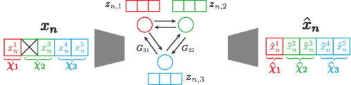
(a)	(b)

Figure 1: (a) Graphic representation of VISL. VISL is a variational auto-encoder based framework. Observations from each group are encoded into low dimensional latent variables. The structure is treated as a global latent variable. A GNN based decoder is used to decode the latent variables to observations. (b) Probabilistic graphical model for VISL, where the partial observation ${\mathbf{x}}$ is generated from its local latent variable ${\mathbf{z}}$ and the global latent variable ${\mathbf{G}}$ which characterizes the structures.

2 Model Description

In the following, we present the formulation of VISL for scalable group-wise structure learning with partial observations using a novel deep generative model based framework.

2.1 Problem setting

Assume a training data set ${\mathbf{X}}=\{{\mathbf{x}}_{n}\}_{n=1}^{N}$ with ${\mathbf{x}}_{n}\in\mathbb{R}^{D}$. The observed and missing values are denoted as ${\mathbf{X}}_{O}$ and ${\mathbf{X}}_{U}$, respectively, where we assume the data are missing completely at random (MCAR) or missing at random (MAR). In Appx. A, we explain how to handle MAR. In particular, variables can be gathered into $M$ pre-defined groups, where each can be denoted as ${\bm{\chi}}_{n,m}=[x_{n,i}]_{i\in\mathcal{I}_{m}}$. $\mathcal{I}_{m}$ containing the variable indices belonging to group $m$ (e.g., $\mathcal{I}_{2}=[4,5,6]$ indicates group $2$ includes the $4^{\text{th}}$, $5^{\text{th}}$ and $6^{\text{th}}$ variables). One should note that each $\mathcal{I}_{m}$ may have varying sizes for different $m$ (i.e. varying group sizes). The goal of VISL is to (i) perform missing value imputation for test samples and (ii) infer structures between groups of variables. We use the adjacency matrix ${\mathbf{G}}\in[0,1]^{M\times M}$ to represent a graph, where $G_{ij}=1$ or $0$ indicates whether there is a directed edge from $i-$th to $j-$th group or not. In the context of the education domain, the above formulation can be rephrased as follows: variable ${\mathbf{x}}_{n}$ containing the student’s responses to a set of questions. $x_{i,j}=1$ represents student $i$ has answered question $j$ correctly. Groups can be defined as the topic associated with each question. $\mathcal{I}_{m}$ contains the question IDs that belong to the same topic, and ${\bm{\chi}}_{m}$ represents a group of responses related to that topic. Clearly, not all students can answer every question. Thus, ${\mathbf{X}}_{O}$, ${\mathbf{X}}_{U}$ represent the existing responses and un-answered questions, respectively. The goal of VISL is to (i) predict students’ responses to un-answered questions, which by itself is important in the education domain (Wang et al., 2020, 2021), and (ii) discover the relationships between topics, which can help education experts optimize the learning experience and the curriculum. For structure learning, we adopt a Bayesian approach for graphs (Heckerman et al., 2006). Namely, we seek to maximize the posterior probability of ${\mathbf{G}}$ given partially observed training data ${\mathbf{X}}_{O}$ within the space of all DAGs:

$${\mathbf{G}}_{\star}= \textstyle\operatorname*{arg\,max}_{{\mathbf{G}}\in\textrm{DAGs}}{\color[rgb]{0,0,1}{\mathrm{p}}({\mathbf{X}}_{O}|{\mathbf{G}}){\mathrm{p}}({\mathbf{G}})}.$$ (1)

To optimize over the structure with the DAG constraint in Eq. 1, we resort to recent continuous optimization techniques (Kyono et al., 2020; Zheng et al., 2018, 2020), where a differentiable measure of ’DAG-ness’, $\mathcal{R}({\mathbf{G}})=\mathrm{tr}(e^{{\mathbf{G}}\odot{\mathbf{G}}})-D-1$, was proposed and is zero if and only if ${\mathbf{G}}$ is a DAG. To leverage this DAG-ness characterisation, we follow Kyono et al. (2020); Yu et al. (2019) and introduce a regulariser based on $\mathcal{R}({\mathbf{G}})$ to favour the DAG-ness of the solution, i.e.

$${\mathbf{G}}_{\star}=\textstyle\operatorname*{arg\,max}_{{\mathbf{G}}}\left({\color[rgb]{0,0,1}{\mathrm{p}}({\mathbf{X}}_{O}|{\mathbf{G}}){\mathrm{p}}({\mathbf{G}})}-\lambda{\color[rgb]{0,0.88,0}\mathcal{R}({\mathbf{G}})}\right).$$ (2)

In the following two sections, we present our detailed formulation, training and imputation algorithms of VISL, that allows the model to infer the latent structure ${\mathbf{G}}$ and impute missing values $\tilde{{\mathbf{x}}}_{U}$ in a test sample $\tilde{{\mathbf{x}}}\in\mathbb{R}^{D}$ based on the observed $\tilde{{\mathbf{x}}}_{O}$.

2.2 Generative model and variational inference

  ${\mathbf{G}}_{ij}\sim\text{Bernoulli}(p_{ij})$

  for $n\in\{1,2,\cdots,N\}$ do

     ${\mathbf{Z}}_{n}\sim\mathcal{N}(\mathbf{0},\sigma_{z}^{2}{\mathbf{I}})$

     ${\mathbf{x}}_{n}\sim\mathcal{N}(f_{\theta}({\mathbf{Z}}_{n},{\mathbf{G}}),\sigma_{x}^{2}{\mathbf{I}})$

  end for

Algorithm 1 Generative process

For the generation of observation ${\mathbf{X}}$, we adopt the latent variable model of Fig. 1. Particularly, given an inferred graph $G$ and latent ${\mathbf{Z}}$, the generative path from ${\mathbf{Z}}$ to ${\mathbf{X}}$ is provided in algorithm 1, where we use a graph neural network (GNN) decoder that respects the learned graph structure $G$ and the provided grouping structure. Then the joint model likelihood is

$${\mathrm{p}}\left({\mathbf{X}},{\mathbf{Z}},{\mathbf{G}}\right)={\mathrm{p}}({\mathbf{G}})\textstyle\prod_{n}{\mathrm{p}}({\mathbf{x}}_{n}|{\mathbf{Z}}_{n},{\mathbf{G}}){\mathrm{p}}({\mathbf{Z}}_{n}).$$ (3)

Amortized variational inference. The true posterior distribution over ${\mathbf{Z}}$ and ${\mathbf{G}}$ in Eq. 3 is intractable since we use a complex deep learning architecture. Therefore, we resort to an efficient amortized variational inference as in Kingma & Welling (2013); Kingma et al. (2019). Here, we consider a fully factorized variational distribution ${\mathrm{q}}({\mathbf{Z}},{\mathbf{G}})={\mathrm{q}}_{\phi}({\mathbf{G}})\prod_{n=1}^{N}{\mathrm{q}}_{\phi}({\mathbf{Z}}_{n}|{\mathbf{x}}_{n})$, where ${\mathrm{q}}_{\phi}({\mathbf{Z}}_{n}|{\mathbf{x}}_{n})$ is a Gaussian whose mean and (diagonal) covariance matrix are given by an encoder. For ${\mathrm{q}}({\mathbf{G}})$, we consider the product of independent Bernoulli distributions over the edges; that is, the presence of each edge from $i$ to $j$ is associated with a probability $p_{ij}$ to be estimated. With the above formulation, the evidence lower bound (ELBO) is

ELBO $$=\textstyle\sum_{n}\left\{\mathbb{E}_{{\mathrm{q}}_{\phi}({\mathbf{Z}}_{n}|{\mathbf{x}}_{n}){\mathrm{q}}({\mathbf{G}})}[\log{\mathrm{p}}({\mathbf{x}}_{n}|{\mathbf{Z}}_{n},{\mathbf{G}})\right.-$$

$$\textrm{KL}[{\mathrm{q}}_{\phi}({\mathbf{Z}}_{n}|{\mathbf{x}}_{n})||{\mathrm{p}}({\mathbf{Z}}_{n})]]\big{\}}-\textrm{KL}[{\mathrm{q}}({\mathbf{G}})||{\mathrm{p}}({\mathbf{G}}))].$$ (4)

Next, we explain our choice of the generator (decoder), which uses a GNN over a learned graph ${\mathbf{G}}$ to model the interactions between latent variables, representing the information about each group. Then, we focus on the inference network (encoder), representing the mapping from the group of observed variables to its corresponding latent representation.

Generator. The generator (i.e., decoder) takes ${\mathbf{Z}}_{n}$ and ${\mathbf{G}}$ as inputs and outputs the reconstructed $\hat{\mathbf{x}}_{n}=f_{\theta}({\mathbf{Z}}_{n},{\mathbf{G}})$, where $\theta$ are the decoder parameters. In order to respect the pre-defined group structure, as shown in Fig. 1, ${\mathbf{Z}}_{n}$ is partitioned into $M$ parts, where ${\mathbf{z}}_{n,m}$ represents the latent variable for the group of observations ${\bm{\chi}}_{n,m}$. This defines a group-wise structured latent space. We adopt a two-step process for the generative path ${\mathbf{Z}}_{n}$ to ${\mathbf{X}}_{n}$: (i) GNN message passing with respect to the learned graph ${\mathbf{G}}$ between latent ${\mathbf{z}}_{n,m}$; (ii) final read-out layer to generate ${\mathbf{X}}_{n}$.

GNN message passing in the generator. In message passing, the information flows between nodes in $T$ consecutive node-to-edge (n2e) and edge-to-node (e2n) operations (Gilmer et al., 2017). At the $t$-th step, we compute an embedding ${\mathbf{h}}^{f}_{i\to j}$ for each edge $i\to j$, called forward embedding, which summarizes the information sent from node $i$ to $j$. Specifically, the n2e/e2n operations in VISL are

$$\textrm{n2e}: \quad{\mathbf{h}}^{(t),f}_{i\to j}=\mathrm{MLP}^{f}\!\left(\left[{\mathbf{z}}_{i}^{(t-1)},{\mathbf{z}}_{j}^{(t-1)}\right]\right),$$ (5)

$$\textrm{e2n}: \quad{\mathbf{z}}_{i}^{(t)}=\mathrm{MLP}^{e2n}\left(\textstyle\sum_{k\neq i}{\mathbf{G}}_{ki}\cdot{\mathbf{h}}_{k\to i}^{(t),f}\right).$$ (6)

Here, $t$ refers to the $t$-th iteration of message passing (that is, ${\mathbf{Z}}^{(0)}={\mathbf{Z}}_{n}$, notice that we omit subindex $n$ for clarity). Finally, $\mathrm{MLP}^{f}$, and $\mathrm{MLP}^{e2n}$ are MLPs to be trained.

Interestingly, the message passing updates indicate that the information flows between latent nodes if a directed edge is specified in graph ${\mathbf{G}}$. Hence, the inferred structure ${\mathbf{G}}$ directly defines relations for latent space ${\mathbf{Z}}$ which contains the information of pre-defined groups. We show that under certain conditions, the inferred graph $G$ also represents the group-wise structure in observational space, and the corresponding model can be reformulated to a general structural equation model (SEM) (Peters et al., 2017) (see Appx. B).

Read-out layer in the generator. After $T$ iterations of GNN message passing, we have ${\mathbf{Z}}^{(T)}$. We then apply a final function that maps ${\mathbf{Z}}^{(T)}$ to the reconstructed $\hat{\mathbf{x}}$, which also respects the pre-defined group structure. Since the observation ${\mathbf{x}}=[{\bm{\chi}}_{1},\ldots,{\bm{\chi}}_{M}]$ may contain ${\bm{\chi}}_{m}$ with different dimensions, we adopt $M$ different MLPs, one for each group as the final read-out layer, to respect the group structure. Namely, $\hat{{\mathbf{x}}}=(g^{1}({\mathbf{z}}_{1}^{T}),\ldots,g^{M}({\mathbf{z}}_{M}^{T}))^{\top},$ where $g^{m}$ represents the MLP for group $m$. Thus, the decoder parameters ${\bm{\theta}}$ include the parameters of the following neural networks: $\textrm{MLP}^{f}$, $\textrm{MLP}^{e2n}$ and $g^{m}$ for $m=1,\ldots,M$.

Inference network. As in standard VAEs, the encoder maps a sample ${\mathbf{x}}_{n}$ to its latent representation ${\mathbf{Z}}_{n}$. As discussed before, ${\mathbf{Z}}_{n}$ is partitioned into $M$ parts, where each ${\mathbf{z}}_{n,m}$ contains the information of the observation in group $m$. Similar to the read-out layer, we utilize the $M$ MLPs to map groups of observations to the mean/variance of the latent variables:

$${\bm{\mu}}_{n} =\left(\mu^{1}_{\phi_{\mu_{1}}}({\bm{\chi}}_{n,1}),\dots,\mu^{M}_{\phi_{\mu_{M}}}({\bm{\chi}}_{n,M})\right)^{\intercal},$$ (7)

$${\bm{\sigma}}_{n} =\left(\sigma^{1}_{\phi_{\sigma_{1}}}({\bm{\chi}}_{n,1}),\dots,\sigma^{M}_{\phi_{\sigma_{M}}}({\bm{\chi}}_{n,M})\right)^{\intercal}.$$

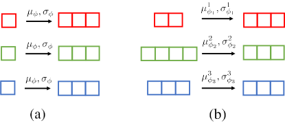
Figure 6: The encoder respects the structure of the latent space. (a) At the level of variables. All the variables use the same encoding functions. (b) At the level of groups of variables. Each group of variables uses different encoding functions.

Here, $\mu^{m}_{\phi_{\mu_{m}}}$ and $\sigma^{m}_{\phi_{\sigma_{m}}}$ are neural networks for group $m$. When missing values are present, we replace them with a constant as in (Nazabal et al., 2020). A graphic representation of how the encoder respects the structure of the latent space is shown in the appendix, Fig. 6(b).

2.3 Training VISL

Given the model described above, we propose the training objective to minimize w.r.t. $\theta$, $\phi$ and ${\mathbf{G}}$:

$$\mathcal{L}_{\textrm{{VISL}}}(\theta,\phi,{\mathbf{G}})={\color[rgb]{0,0,1}-\mathrm{ELBO}}+\lambda{\color[rgb]{0,0.88,0}\mathbb{E}_{{\mathrm{q}}({\mathbf{G}})}\left[\mathcal{R}({\mathbf{G}})\right]},$$ (8)

where ELBO is given by Sec. 2.2 and the DAG regulariser $\mathcal{R}({\mathbf{G}})$ was introduced in Eq. 2 to favor the DAG-ness of learned graph ${\mathbf{G}}$.

Evaluating the training loss $\mathcal{L}_{\textrm{{VISL}}}$. VISL can work with any type of data. The log-likelihood term ($\log p_{\theta}({\mathbf{x}}_{n}|{\mathbf{Z}}_{n},{\mathbf{G}})$ in Sec. 2.2) is defined according to the data type. We use a Gaussian likelihood for continuous variables and a Bernoulli likelihood for binary ones. For the inference of ${\mathbf{Z}}$ and ${\mathbf{G}}$, the standard reparametrization trick is used to sample ${\mathbf{Z}}_{n}$ from the Gaussian ${\mathrm{q}}_{\phi}({\mathbf{Z}}_{n}|{\mathbf{x}}_{n})$ (Kingma & Welling, 2013; Kingma et al., 2019). To backpropagate the gradients through the discrete variable ${\mathbf{G}}$, we resort to the Gumbel-softmax trick to sample from ${\mathrm{q}}({\mathbf{G}})$ (Jang et al., 2017; Maddison et al., 2017). The $\textrm{KL}[{\mathrm{q}}_{\phi}({\mathbf{Z}}_{n}|{\mathbf{x}}_{n})||{\mathrm{p}}({\mathbf{Z}}_{n})]$ and $\textrm{KL}[{\mathrm{q}}({\mathbf{G}})||{\mathrm{p}}({\mathbf{G}}))]$ terms can be obtained in closed-form since they are Gaussian distributions and independent Bernoulli distributions over the edges, respectively. This formulation brings additional advantages in real-life applications since one can easily incorporate domain knowledge and prior information into the VISL framework. For example, if the existence of a specific edge is known a priori, the edge probability can be set to 0/1 in the prior distribution. Finally, the DAG-loss regulariser in Eq. 8 can be computed by evaluating the function $\mathcal{R}$ on a Gumbel-softmax sample from ${\mathrm{q}}({\mathbf{G}})$. To adapt the model to different missing levels in the training data ${\mathbf{X}}$, we adopt the masking strategy (Ma et al., 2019; Gong et al., 2019), which drops a random percent of the observed values during training. The entire training procedure for VISL is summarised in Algorithm 2.

Input : Training dataset ${\mathbf{X}}$, possibly with missing values.

for each batch of samples $\{{\mathbf{x}}_{n}\}_{n\in B}$ do

       Drop a percentage of the data for each sample ${\mathbf{x}}_{n}$.;

      

      Encode ${\mathbf{x}}_{n}$ through the reparametrization trick to sample ${\mathbf{Z}}_{n}\sim\mathcal{N}(\bm{\mu}_{\phi}({\mathbf{x}}_{n}),\bm{\sigma}_{\phi}^{2}({\mathbf{x}}_{n}))$ using Eq.7.;

      

      Use the Gumbel-softmax to sample ${\mathbf{G}}$ from ${\mathrm{q}}({\mathbf{G}})$.;

      

      Use decoder to reconstruct $\hat{\mathbf{x}}_{n}=f_{\theta}({\mathbf{Z}}_{n},{\mathbf{G}})$.;

      

      Calculate the training loss $\mathcal{L}_{\textrm{{VISL}}}$ (Eq. 8).;

      

      Gradient step w.r.t. $\phi$ (encoder parameters), $\theta$ (decoder parameters) and ${\mathbf{G}}$ (posterior edge probabilities).;

      

Output : Encoder parameters $\phi$, decoder parameters $\theta$, and posterior probabilities over the edges ${\mathbf{G}}$.

Algorithm 2 Training VISL.

Two-step training. After training, we obtain the posterior of the graph ${\mathbf{G}}$, which respects the underlying structure of the groups as shown in Appx. B. With the trained network, we can impute missing values in the groups where their ancestors contain some observations but if a group has no ancestors no information can be propagated during imputation. After learning the graph structure and to facilitate the imputation task, we introduce a backwards edge: for an edge from $j$ to $i$ we denote the backwards edge information as ${\mathbf{h}}^{b}_{i\to j}$ which codifies the information that the $i\to j$ edge lets flow from the $j$-th to the $i$-th node. It is defined in the same way as Eq. 5, i.e.,: ${\mathbf{h}}^{(t),b}_{i\to j}=\mathrm{MLP}^{b}\!\left(\left[{\mathbf{z}}_{i}^{(t-1)},{\mathbf{z}}_{j}^{(t-1)}\right]\right)$, where $\mathrm{MLP}^{b}$ is the backward MLP; and the e2n update (Eq.6) is modified to ${\mathbf{z}}_{i}^{(t)}=\mathrm{MLP}^{e2n}\left(\textstyle\sum_{k\neq i}{\mathbf{G}}_{ki}\cdot\left\{{\mathbf{h}}_{k\to i}^{(t),f}+{\mathbf{h}}_{i\to k}^{(t),b}\right\}\right)$.

In summary, we propose a two-stage training process, where the first stage — described in previous sections — focuses on discovering the edge directions between nodes without the $\mathrm{MLP}^{b}$ (i.e., we do not train the $\mathrm{MLP}^{b}$). In the second stage, we fix the graph structure ${\mathbf{G}}$ and continue to train the model with the backward MLP. This two-stage training process allows VISL to leverage the backward MLP for the imputation task without updating the graph structure.

Revisiting the learning objectives. The optimal graph of relationships, denoted as ${\mathbf{G}}_{\star}$ in Eq. 2, is given by the estimated posterior probabilities of graph ${\mathbf{G}}$. In addition, the regularizer $\mathcal{R}({\mathbf{G}})$ provides a way to evaluate if the resulting graph is a DAG. By tuning the regularizer strength $\lambda$, one can ensure that the resulting ${\mathbf{G}}^{*}$ represents a proper DAG.

For imputation, similar to Ma et al. (2019); Nazabal et al. (2020), the trained model can impute missing values for a test instance $\widetilde{\mathbf{x}}$ as

$${\mathrm{p}}(\widetilde{\mathbf{x}}_{U}|\widetilde{\mathbf{x}}_{O},{\mathbf{X}})=\mathbb{E}_{{\mathrm{q}}_{\phi}({\mathbf{Z}}|\widetilde{\mathbf{x}}){\mathrm{q}}({\mathbf{G}})}{\mathrm{p}}(\widetilde{\mathbf{x}}_{U}|{\mathbf{Z}},{\mathbf{G}}).$$ (9)

Therefore, the distribution over $\widetilde{\mathbf{x}}_{U}$ (missing values) is obtained by applying the encoder and decoder with $\widetilde{\mathbf{x}}$ as input. One important distinction of VISL compared to Ma et al. (2019); Nazabal et al. (2020) is that it incorporates the learned structure ${\mathbf{G}}$ into the imputation, which helps the model avoid over-fitting due to spurious correlations (Kyono et al., 2020).

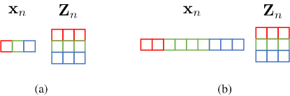
Figure 5: Structured latent space. (a) At the level of variables. Each variable in ${\mathbf{x}}_{n}$ (each color) has its own latent subspace, which is given by a row in ${\mathbf{Z}}_{n}$. (b) At the level of groups of variables. Here, each group of variables (each color) has its own latent subspace, which is given by a row in ${\mathbf{Z}}_{n}$.

Special case: variable-wise relations. In the above formulation, we have defined VISL for group-wise structure learning. Variable-wise relations can be regarded as a special case. In particular, we can set $M=D$ and $\mathcal{I}_{m}=\{m\}$ (see Fig. 5 (a) in the appendix), i.e. each group only contains a single variable. Through this modification, we can further simplify the encoder and read-out layer. Instead of using $M$ different MLPs, a single MLP can be shared across all variables since each group has dimension of 1. The mean function for the encoder is then defined as

$$\bm{\mu}_{n}=\left(\mu_{\phi}(x_{n,1}),\ldots,\mu_{\phi}(x_{n,D})\right).$$ (10)

One can define encoder variance $\bm{\sigma}$ (Fig. 6 (a) in the appendix) and the read-out layer $g$ analogously.

3 Related Work

Since VISL simultaneously tackles missing value imputation and structure learning, we review both fields. Moreover, we review recent works that utilize structure learning to improve the performance of another deep learning task, similar to VISL. Finally, as one of the focused applications of this work is in the education domain, we review recent advances of AI in education.

Structure learning. Structure learning aims to infer the underlying structures associated with some observations. There are mainly three types of methods: constrained-based, score-based, and hybrid. Constraint-based ones exploit (conditional) independence tests to find the underlying structure, such as PC (Spirtes & Glymour, 1991) and Fast Causal Inference (FCI) (Spirtes et al., 2000). They have recently been extended to handle partially observed data through test-wise deletion and adjustments (Strobl et al., 2018; Tu et al., 2019a). Score-based methods find the structure by optimizing a proper scoring function. The core difficulty lies in the number of possible graphs growing super-exponentially with the number of nodes (Chickering et al., 2004). Thus, explicitly solving the optimization can only be done up to a few nodes (Ott & Miyano, 2003; Singh & Moore, 2005; Cussens et al., 2017), resulting in significant limitations in scalability. Therefore, approximation methods have been proposed to ease the computational burden, including searching over topological ordering (Teyssier & Koller, 2012; Scanagatta et al., 2015, 2016), greedy search (Chickering, 2002; Ramsey et al., 2017), coordinate descent (Fu & Zhou, 2013; Aragam & Zhou, 2015; Gu et al., 2019).

Recently, continuous optimization of structures, called Notears, has become very popular within score-based methods (Zheng et al., 2018). Notears proposed a differentiable algebraic characterization of the DAG, allowing an equality-constrained optimization problem to learn the model parameters and graph structures jointly. Notears has inspired the development of other methods, Notears-MLP and Notears-Sob (Zheng et al., 2020), Grandag (Lachapelle et al., 2019), and DAG-GNN (Yu et al., 2019), which extend the original formulation to model nonlinear relationships between variables. However, their formulations cannot handle missing values and have been observed to be sensitive to data scaling (Kaiser & Sipos, 2021). In particular, DAG-GNN also adopts a specially-designed GNN to perform structure learning (Yu et al., 2019). Compared to our formulation, there are three key distinctions: (i) our model is designed to discover the group-wise relationship, while DAG-GNN and other structured discovery methods focus on variables level structure learning; (ii) our model is capable of performing missing value imputation and group-wise structure learning simultaneously, whereas the original formulation of DAG-GNN and related work can only handle complete data; (iii) VISL adopts Bayesian learning for the underlying graphs, whereas DAG-GNN uses a point estimation.

Structure deep learning. Continuous optimization for learning structures has been used to boost performance in classification. In CASTLE (Kyono et al., 2020), structure learning is introduced as a regulariser for a deep learning classification model. This regulariser reconstructs only the most relevant causal features, leading to improved out-of-sample predictions. In SLAPS (Fatemi et al., 2021), the classification objective is supplemented with a self-supervised task that learns a graph of interactions between variables through a GNN. However, these works focused on the supervised classification task, and they did not advance the performance of the structure learning itself.

Missing values imputation. The relevance of missing data in real-world problems has motivated a long history of research (Dempster et al., 1977; Rubin, 1976). A popular approach for this task is to estimate the missing values based on the observed ones through different techniques (Scheffer, 2002). Here, we find popular methods such as missforest (Stekhoven & Bühlmann, 2012), which relies on Random Forest, and MICE (Buuren & Groothuis-Oudshoorn, 2010), which is based on Bayesian Ridge Regression. Also, the efficiency of amortized inference in generative models has motivated its use for missing values imputation. This is explored in Wu et al. (2018), although fully observed training data is required. This limitation is addressed in both Nazabal et al. (2020), where a zero-imputation strategy is used for partially observed data, and Ma et al. (2019), where a permutation invariant set encoder is utilized to handle missing values. VISL also leverages amortized inference, although the discovered relationships inform the imputation through a GNN.

AI in education. Recently, there has been tremendous progress in using AI for educational applications. For example, knowledge training (Lan et al., 2014; Vie & Kashima, 2019; Naito et al., 2018), which focuses on tracking the evolution of the knowledge of some students; grading students’ performance (Waters et al., 2015); generating feedback for students working on coding challenges (Wu et al., 2019). In particular, most related to VISL is work on imputing missing values in students’ responses to questions. Wang et al. (2020) adopts a partial VAE (Ma et al., 2019) to perform missing value imputation and personalization. However, partial VAE does not consider the structural relations between questions/topics and cannot perform structure learning. With the additional insights from structure learning, VISL can provide more information to teachers to help curriculum design than just imputations.

(a)	(b)

Figure 2: (a): Structure simulated for one of the synthetic datasets with 5 variables. (b): Graph predicted by VISL (when the one on the left is used as the true one). VISL predicts all the true relationships plus some additional ones (dashed edges).

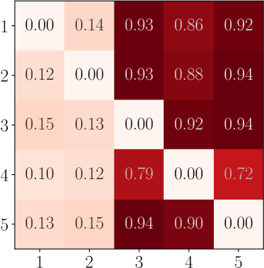
Figure 3: Probability of edges obtained by VISL in the synthetic experiment. By using a 0.5 threshold, we get the predicted graph in Fig. 2(b). Item $(i,j)$ refers to the probability of edge $i\to j$.

	RMSE
Majority vote	0.5442$\pm$0.0032
Mean imputing	0.2206$\pm$0.0061
MICE	0.1361$\pm$0.0046
Missforest	0.1313$\pm$0.0025
PVAE	0.1407$\pm$0.0043
VISL	0.1196$\pm$0.0024

Table 1: Imputation results for the synthetic experiment. Mean and standard error over 15 datasets.

	Adjacency			Orientation			Causal accuracy
	Recall	Precision	F1-score	Recall	Precision	F1-score
PC	0.422$\pm$0.056	0.634$\pm$0.067	0.495$\pm$0.056	0.218$\pm$0.046	0.328$\pm$0.061	0.257$\pm$0.051	0.33$\pm$0.046
GES	0.452$\pm$0.044	0.569$\pm$0.036	0.491$\pm$0.038	0.249$\pm$0.046	0.305$\pm$0.053	0.270$\pm$0.049	0.364$\pm$0.045
NOTEARS (L)	0.193$\pm$0.028	0.443$\pm$0.059	0.265$\pm$0.036	0.149$\pm$0.023	0.367$\pm$0.060	0.209$\pm$0.032	0.149$\pm$0.023
NOTEARS (NL)	0.328$\pm$0.039	0.489$\pm$0.051	0.387$\pm$0.044	0.277$\pm$0.032	0.417$\pm$0.043	0.327$\pm$0.035	0.277$\pm$0.032
DAG-GNN	0.443$\pm$0.064	0.509$\pm$0.062	0.464$\pm$0.061	0.352$\pm$0.050	0.415$\pm$0.052	0.373$\pm$0.049	0.352$\pm$0.050
VISL	0.843$\pm$0.043	0.679$\pm$0.037	0.740$\pm$0.033	0.520$\pm$0.067	0.414$\pm$0.058	0.454$\pm$0.060	0.726$\pm$0.069

Table 2: Causal discovery results for synthetic experiment (mean and std error over 15 datasets).

	Adjacency			Orientation			Causal Accuracy
	Recall	Precision	F1-score	Recall	Precision	F1-score
PC	0.046$\pm$0.001	0.375$\pm$0.006	0.082$\pm$0.001	0.024$\pm$0.001	0.199$\pm$0.011	0.044$\pm$0.002	0.058$\pm$0.003
GES	0.110$\pm$0.001	0.436$\pm$0.008	0.176$\pm$0.002	0.082$\pm$0.001	0.323$\pm$0.009	0.131$\pm$0.003	0.121$\pm$0.001
NOTEARS (L)	0.006$\pm$0.000	0.011$\pm$0.001	0.008$\pm$0.000	0.001$\pm$0.000	0.001$\pm$0.001	0.001$\pm$0.000	0.001$\pm$0.000
NOTEARS (NL)	0.011$\pm$0.001	0.644$\pm$0.025	0.022$\pm$0.002	0.006$\pm$0.001	0.354$\pm$0.018	0.012$\pm$0.001	0.006$\pm$0.001
DAG-GNN	0.129$\pm$0.028	0.272$\pm$0.101	0.128$\pm$0.027	0.051$\pm$0.010	0.126$\pm$0.059	0.050$\pm$0.007	0.051$\pm$0.010
VISL	0.261$\pm$0.006	0.637$\pm$0.009	0.370$\pm$0.005	0.236$\pm$0.007	0.573$\pm$0.005	0.334$\pm$0.006	0.245$\pm$0.006

Table 3: Structure discovery results for neuropathic pain data (mean and std error over five runs).

4 Experiments

We evaluate the performance of VISL in three different problems: a synthetic experiment where the data generation process is controlled, a semi-synthetic problem (simulated data from a real-world problem) with many more variables (Neuropathic Pain), and the real-world problem that motivated the development of the group-level structure learning (Eedi). To compare the model performance with related work, the first two datasets are on the variable level, which means that each group only has one variable. In the education setting, we focus on the real-world usage of the method and have worked closely with the domain expert to evaluate the results. Additional experiments are presented in the appendix.

Baselines. We consider five baselines for the structure discovery task at the variable level. PC (Spirtes et al., 2000) and GES (Chickering, 2002) are the most popular methods in constraint-based and score-based approaches, respectively. We also consider three recent algorithms based on continuous optimization and deep learning: NOTEARS (Zheng et al., 2018), the non-linear (NL) extension of NOTEARS (Zheng et al., 2020), and DAG-GNN (Yu et al., 2019). Unlike VISL, these baselines cannot deal with missing values in the training data. Therefore, we work with fully observed training data in the first two sections when using these baselines. In contrast, the real-world data in the last section comes with partially observed training data, and the goal is to discover group-wise relationships. These baselines are not applicable. For the missing data imputation task, we also consider five baselines. Mean Imputing and Majority Vote are popular techniques used as references, Missforest (Stekhoven & Bühlmann, 2012) and MICE (Buuren & Groothuis-Oudshoorn, 2010) are two of the most widely-used imputation algorithms, and PVAE (Ma et al., 2019) is a recent algorithm based on amortized inference.

Metrics. Imputation performance is evaluated with standard metrics such as RMSE (continuous variables) and accuracy (binary variables). For binary variables , we also provide the area under the ROC and the Precision-Recall curves (AUROC and AUPR, respectively), which are especially useful for imbalanced data (such as Neuropathic Pain). We follow common practice (Glymour et al., 2019; Tu et al., 2019a) regarding structure discovery performance, and consider metrics on the adjacency and orientation. While the former does not take into account the direction of the edges, the latter does. For both adjacency and orientation, we compute recall, precision and F₁-score. We also provide causal accuracy, a popular structure discovery metric that considers edge orientation (Claassen & Heskes, 2012).

4.1 Synthetic experiment

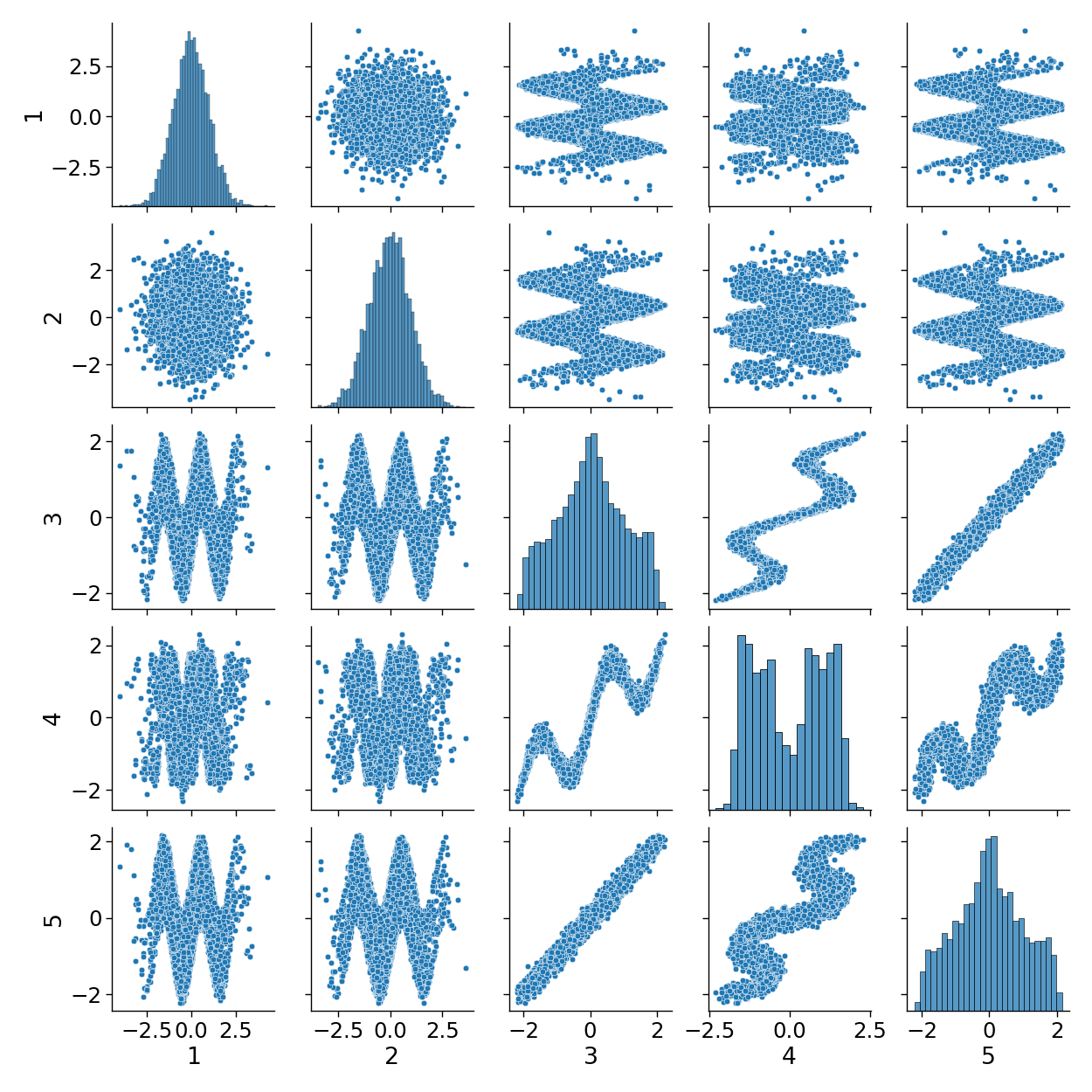
Figure 7: Pair-plot for the dataset generated from the graph in Fig. 2(a) in the paper. We observe different type of relationships between variables, including non-linear ones.

We simulate fifteen synthetic datasets. For each simulated dataset, we first sample the true structure ${\mathbf{G}}$; see Fig. 2(a) for an example. We obtain the samples of the datasets by computing each variable based on its parents using a non-linear mapping based on the $\sin$ function. The appendix provides further details, including a visualisation of the generated data in Fig. 7. For each dataset, we simulate $5000$ training and $1000$ test samples.

Imputation performance. VISL outperforms the baselines in terms of imputation across all synthetic datasets ( Table 1).The results grouped by the number of variables are presented by Table 8 in the appendix. Therefore, VISL exploits the learned graph to improve imputation by avoiding spurious correlations.

Structure discovery performance. VISL obtains better performance than the baselines, see Table 2. The results split by the number of variables are shown in the appendix, Table 10. Notice that NOTEARS (NL) is slightly better in terms of orientation precision. However, this is at the expense of a significantly lower capacity to detect true edges; see the recall and the trade-off between both (F₁-score). In this small synthetic experiment, it is possible to visually inspect the predicted graph. Fig. 3 shows the posterior probability of each edge (i.e. the estimated matrix ${\mathbf{G}}$) for the simulated dataset that uses the true graph in Fig. 2(a). Using a threshold of 0.5, we obtain the predicted graph in Fig. 2(b). We observe that all the true edges are captured by VISL, with some additional edges due to finite data and non-convex optimization.

Finally, VISL can scale to large data both in terms of data points (which benefits naturally from its SGD-based optimization) and dimensionality (thanks to the continuous optimization over the graph space). We demonstrate the computational efficiency with synthetic data ranging from 4 nodes to 512 nodes in the appendix, Table 11.

4.2 Neuropathic pain dataset

	Accuracy	AUROC	AUPR
Majority vote	0.9268$\pm$0.0003	0.5304$\pm$0.0003	0.3366$\pm$0.0025
Mean imputing	0.9268$\pm$0.0003	0.8529$\pm$0.0012	0.3262$\pm$0.0034
MICE	0.9469$\pm$0.0007	0.9319$\pm$0.0010	0.6513$\pm$0.0046
Missforest	0.9305$\pm$0.0004	0.8915$\pm$0.0093	0.5227$\pm$0.0033
PVAE	0.9415$\pm$0.0003	0.9270$\pm$0.0007	0.5934$\pm$0.0046
VISL	0.9471$\pm$0.0006	0.9392$\pm$0.0008	0.6597$\pm$0.0053

Table 4: Imputation results for neuropathic pain data (mean and std error over five runs).

We evaluate our method using a machine learning benchmark in healthcare applications (Tu et al., 2019b). The dataset contains records of patients regarding the symptoms associated with neuropathic pain. There are 222 variables in this dataset. Unlike the previous experiment with continuous data, this dataset has binary variables indicating the symptoms. The train and test sets have $1000$ and $500$ patients, respectively.

Imputation performance. VISL shows competitive or superior performance when compared to the baselines, see Table 4. Notice that AUROC and AUPR allow for an appropriate threshold-free assessment in this imbalanced scenario. Indeed, as expected from medical data, the minority of values are 1 (symptoms); here, the prevalence of symptoms is around $8\%$ in the test set. Interestingly, it is precisely in AUPR where the differences between VISL and the rest of the baselines are larger except MICE, whose performance is very similar to that of VISL in this dataset.

Structure discovery results. As in the synthetic experiment, VISL outperforms the causality-based baselines; see Table 3. Notice that NOTEARS (NL) is slightly better in terms of adjacency-precision, i.e. the edges that it predicts are slightly more reliable. However, this is at the expense of a significantly lower capacity to detect true edges, see the recall and the trade-off between both (F₁-score).

4.3 Eedi topics dataset

Finally, we evaluate our method on an even more challenging real-world dataset in education requiring group-wise structure discovery. This is an important real-world problem in the field of AI-powered educational systems (Wang et al., 2021, 2020). In this setting, we are interested in relationships between topics while the observations are question-answer pairs under these topics. The dataset is very sparse, with 74.1% of the values missing. The dataset contains the responses by 6147 students to 948 mathematics questions. The 948 variables are binary (1 if the student provided the correct answer and 0 otherwise). These 948 questions target very specific mathematical concepts and are grouped within a meaningful hierarchy of topics; see Fig. 4. Here we apply our proposed model to find the relationships among the topics using the third level of the topic hierarchy (Fig. 4), resulting in 57 group-level nodes.

Figure 4: Hierarchy of topics in Eedi data. All the questions are related to maths (level 0 topic). The number of topics at levels 1, 2 and 3 are 3, 25 and 57. Each question is associated with only one topic at level 3 (thus, to only one topic at any higher level).

	Accuracy	AUROC	AUPR
Majority vote	0.6260$\pm$0.0000	0.6208$\pm$0.0000	0.7465$\pm$0.0000
Mean imputing	0.6260$\pm$0.0000	0.6753$\pm$0.0000	0.6906$\pm$0.0000
MICE	0.6794$\pm$0.0005	0.7453$\pm$0.0007	0.7483$\pm$0.0010
Missforest	0.6849$\pm$0.0005	0.7219$\pm$0.0007	0.7478$\pm$0.0008
PVAE	0.7138$\pm$0.0005	0.7852$\pm$0.0001	0.8204$\pm$0.0002
VISL	0.7147$\pm$0.0007	0.7815$\pm$0.0008	0.8179$\pm$0.0006

Table 5: Imputation results for Eedi topics dataset (mean and standard error over five runs).

	Adjacency		Orientation
	Expt 1	Expt 2	Expt 1	Expt 2
Random	2.04	2.08	1.44	1.40
DAG-GNN	2.04	2.32	1.68	1.68
VISL	3.60	3.70	2.76	2.60

Table 6: Average expert evaluation of the topic relationships. Cohen’s $\kappa$ inter-annotator agreement is $0.72$ for adjacency and $0.76$ for orientation (substantial agreement).

VISL Number Algebra Geometry Number 30 4 3 Algebra 2 6 0 Geometry 0 0 5

DAG-GNN Number Algebra Geometry Number 8 3 6 Algebra 1 5 2 Geometry 14 7 11

Random Number Algebra Geometry Number 7 4 6 Algebra 8 1 6 Geometry 6 3 9

Table 7: Distribution of the relationships across level 1 topics.The item $(i,j)$ refers to edges in the direction $i\to j$.

Imputation results. VISL achieves competitive or superior performance when compared to the baselines (Table 5). Although the dataset is relatively balanced (54% of the values are 1), we provide AUROC and AUPR for completeness. Notice that this setting is more challenging than the previous ones since we learn relationships between groups of variables (topics). Indeed, whereas the group extension allows for more meaningful relationships, the information flow happens at a less granular level. Interestingly, even in this case, VISL obtains similar or improved imputation results compared to the baselines.

Structure discovery results between groups. Most of the baselines used so far cannot be applied here because i) they cannot deal with partially observed training data or ii) they cannot learn relationships between groups of variables. DAG-GNN is the only one that can be adapted to satisfy both properties. For the first one, we adapt DAG-GNN following the same strategy as in VISL, i.e. replacing missing values with a constant value. For the second one, notice that DAG-GNN can be used for vector-valued variables according to the original formulation (Yu et al., 2019). However, all of them need to have the same dimensionality. To cope with arbitrary groups, we apply the group-specific mappings described for VISL. Finally, as an additional reference, we also compare with randomly generated relationships, which we refer to as Random.

Moreover, as there are no ground truth relationships in this real-world application, we ask two experts (teachers) to assess the validity of the relationships found by VISL, DAG-GNN, and Random. For each relationship, they evaluate the adjacency (whether it is sensible to connect the two topics) and the orientation (whether the first one is a prerequisite for the second one). They provide an integer value from 1 (strongly disagree) to 5 (strongly agree), i.e. the higher, the better. The complete list of relationships and expert evaluations for VISL, DAG-GNN, and Random can be found in the appendix; see Table 15, Table 16, and Table 17, respectively. In summary, Table 6 shows here the average evaluations: we see that the relationships discovered by VISL score much more highly across both metrics than the baseline models.

Another interesting aspect is how the relationships between level-3 topics are distributed across higher-level topics (recall Fig. 4). Intuitively, it is expected that most of the relationships happen inside higher-level topics (e.g. Number-related concepts are more probably related to each other than to Geometry-related ones). Table 7 shows such a distribution for the compared methods. Indeed, notice that the percentage of inside-topic relationships is higher for VISL (82%) and DAG-GNN (42%) than for Random (34%). An analogous analysis for the 25 level-2 topics is provided in the appendix; see Table 12 (VISL), Table 13 (DAG-GNN), and Table 14 (Random). In particular, whereas 6% of the connections happen inside level 2 topics for Random, it is 14% for DAG-GNN and 36% for VISL.

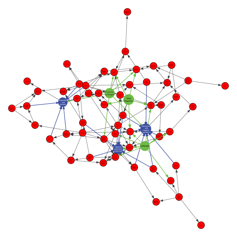
Figure 8: The structures discovered by VISL based on an alternative education dataset. In particular, the blue node represents the curriculum that should be taught later. On the other hand, the green node represents the fundamental topics that should be taught earlier.

Education Impact. Lastly, to make a real-world impact, we have been provided with an additional education dataset in the same format as Eedi by an education organization to help provide insight for math curriculum building. The final structure among all topics found by VISL is presented by figure Fig. 8 in the appendix. The predicted relationships allowed insights into which topics are foundational and need to be covered earlier (topics with many originating edges), as well as which topics are more complex and should be covered later (topics with many incoming edges). This allowed us to re-evaluate the order of topics in a nationwide used secondary curriculum. Specifically, topics such as “arithmetic” or “properties of shapes” were moved earlier in the curriculum, while topics such as “negative numbers” or “proportion and similarity” were moved to a later stage in the curriculum. Another interesting example found by the domain expert is the Venn diagram, which was originally taught in year 9/10 and is now suggested to move to year 7. Experts found that the Venn diagram has been a useful tool in teaching other topics which are currently taught before year 10. Moving this earlier will help students to learn other topics better. This emphasises the real-world impact our model, VISL, can have in planning curricula.

5 Conclusions

We introduced VISL, a novel approach that simultaneously performs group-wise structure discovery and learns to impute missing values. Both tasks are performed jointly: imputation is informed by the discovered relationships and vice-versa, leading to improved performance for both tasks. Moreover, motivated by a real-world problem, VISL shows its impact in the real-world education domain to aid domain experts in setting up curriculum.

Appendix A VISL for missing-at-random scenario

In this section, we briefly explain why VISL can handle MAR problem by leveraging the results from Rubin (1976). Let’s denote $\bm{r}_{i}$ as the missing mask, where $r_{i,d}=1$ indicates $x_{i,d}$ is observed. For the random variable $R$, we use $p_{\lambda}(\bm{r}|{\mathbf{x}})$ as the missing mechanism with parameters $\lambda$. To explicitly state the dependence of VISL and its model parameter $\theta$, we use $p_{\theta}({\mathbf{x}})$ to denote the corresponding model density. We can now formally define the concept of MAR.

Definition A.1 (Missing at Random (Rubin, 1976)).

The missing data are missing at random if for each value of $\lambda$, $p_{\lambda}(\bm{r}|{\mathbf{x}})$ takes teh same value for all ${\mathbf{x}}_{u}$. Namely, $p_{\lambda}(\bm{r}|{\mathbf{x}})=p_{\lambda}(\bm{r}|{\mathbf{x}}_{o})$.

Recall that our VISL is trained by maximizing the ELBO (Eq.2.2) based on the observed values $x_{o}$. However, this formulation ignores the missing mechanisms $p_{\phi}(\bm{r}|{\mathbf{x}})$. In order to perform missing value imputation, one need to ensure that the inference for $\theta$ should be correct. In the following, we show under MAR, ignoring missing mechanism does not affect the correctness of inferring $\theta$ under ELBO. The following proof is an adaptation of Theorem 7.1 in Rubin (1976).

When explicitly modelling the missing mechanism, the joint likelihood can be written as

$$\log p_{\theta,\phi}({\mathbf{x}}_{o},\bm{r})$$

$$=\log\int p_{\theta}({\mathbf{x}})p_{\phi}(\bm{r}|{\mathbf{x}})d{\mathbf{x}}_{u}$$

$$=\log\int p_{\theta}({\mathbf{x}},\bm{z},\bm{G})p_{\phi}(\bm{r}|{\mathbf{x}})d\bm{z}d\bm{G}d{\mathbf{x}}_{u}$$

$$=\log p_{\phi}(\bm{r}|{\mathbf{x}}_{o})\int p_{\theta}({\mathbf{x}},\bm{z},\bm{G})d\bm{z}d\bm{G}d{\mathbf{x}}_{u}$$

$$\geq\log p_{\phi}(\bm{r}|{\mathbf{x}}_{o})+\text{ELBO}(\theta)$$

where the third equality is from the definition of MAR and the last inequality is from the standard ELBO derivation. The above equation explicitly lower bounds the joint likelihood by two separate terms regarding $\theta$ and $\phi$. Thus, when performing inference over $\theta$, one can safely ignore the missing mechanism involving $\phi$, resulting in the same optimization objective as Eq.2.2.

Appendix B Does VISL respect the graph G in observational space

From the formulation of the decoder in VISL (Eq.5 and 6), the inferred graph ${\mathbf{G}}$ seems to define whether the information flow between nodes is allowed or not. Namely, when $G_{ij}=1$, the information is allowed to pass from $z_{i}$ to $z_{j}$ at each iteration $t$. Thus, ${\mathbf{G}}$ directly defines a structure for latent space ${\mathbf{Z}}$, and indirectly defines a structure in observation ${\mathbf{X}}$ through the GNN updates and the final read-out layer. A natural question to ask is whether the resulting observations ${\mathbf{x}}$ from VISL also respect the graph ${\mathbf{G}}$. In the following, we show that when GNN is in equilibrium and the read-out layer is invertible without additional observational noise ($\sigma_{x}=0$), the VISL is in fact a SEM for observation ${\mathbf{x}}$, which respects the graph ${\mathbf{G}}$. In the following, for the clarity of notations, we consider the structure learning between variables. For group-wise relations, it is trivial to generalize, since the going from variable-wise to group-wise only changes the read-out layer, where we use $M$ different MLPs instead of one.

First, let’s clarify what do we mean by ”respect a graph ${\mathbf{G}}$”.

Definition B.1 (Respect a graph ${\mathbf{G}}$).

For a given VISL model $p({\mathbf{x}},{\mathbf{z}};{\mathbf{G}})$ with a specific graph ${\mathbf{G}}$, we say the model $p({\mathbf{x}};{\mathbf{G}})=\int p({\mathbf{x}},{\mathbf{z}};{\mathbf{G}})d{\mathbf{z}}$ respects the graph ${\mathbf{G}}$ if it can be factorized

$$p({\mathbf{x}};{\mathbf{G}})=\prod_{d=1}^{D}p(x_{d}|PA(d);{\mathbf{G}}),$$

where $PA(d)$ is a set of parents of node $i$ specified by graph ${\mathbf{G}}$.

B.1 GNN at steady state

From the GNN message passing equations, we can re-organize Eq.5 and 6 into one equation:

$$z_{i}^{t}=F(PA(i)^{t-1},z_{i}^{t-1}),$$ (11)

where $PA(i)^{t-1}$ is a set of parents’ value for node $i$ at iteration $t-1$, $z_{i}^{t}$ is the value for node $i$ at iteration t and $F(\cdot)$ represents the GNN message passing updates.

The above equation resembles a fixed-point iteration procedure for function $F$. Indeed, under the context of GNN, this has been considered as a standard procedure to search for the equilibrium state due to its exponential convergence (Dai et al. 2018, Eq.1; Gu et al. 2020, Eq.2(b)). Thus, we assume that the GNN updates $F$ has unique equilibrium states given the initial conditions $AN(i)^{0}\cup z_{i}^{0}$ for each $i$, where $AN(i)^{0}$ represents the initial values of ancestors for node $i$. For a sufficient condition of its existence, one can refer to Gu et al. (2020, Theorem 4.1). We note that this is only a sufficient condition, meaning that the GNN without the conditions in Gu et al. (2020) can still have equilibrium states. Since discussing a necessary and sufficient conditions for the existence of the equilibrium state is out of the scope of this paper, we simply made an assumption that function $F$ has steady states. The reason we consider the initial ancestor values rather than just parent values is due to the message passing nature, where the value $PA(i)^{t}$ contains the information from the nodes that is at most $t$-hops away.

Since graph $G$ represents a DAG, one can always find a permutation $\pi$ of the original index $i=1,\ldots,D$ based on the topological order. For concise notations, we assume the identity permutation. When the GNN is in equilibrium, we can rewrite Eq.11 as

$$z_{i}^{\infty}=F(PA^{\infty}(i),z_{i}^{\infty}),$$ (12)

where the superscript $\infty$ represents that steady state of the node. From the assumption, since the steady state for each $z_{i}^{\infty}$ depends on the initial values $AN(i)^{0}\cup z_{i}^{0}$, it is trivial to see that the steady state $PA^{\infty}(i)$ depends on $AN^{0}(i)$. Therefore, the steady state $z_{i}^{\infty}$ is uniquely determined by $PA^{\infty}(i)$ and $z_{i}^{0}$. Namely,

$$z_{i}^{\infty}=H_{i}(PA^{\infty}(i),z_{i}^{0})$$ (13)

for $i=1,\ldots,D$, where $H_{i}$ is a mapping from $PA(i)^{\infty}$ and $z_{i}^{0}$ to the steady state of node $i$.

This is exactly the general form of an structural equation model (SEM) defined by graph $G$. If we further assume that the read-out layer $g(\cdot)$ is invertible, we can obtain

$$x_{i}=g\left(H_{i}\left(g^{-1}\left(PA^{\infty}_{x}(i)\right),z_{i}^{0}\right)\right),$$ (14)

which is also an SEM based on $G$ for observation ${\mathbf{x}}$. Thus, it is trivial that VISL respects the graph $G$ based on the above assumptions.

In practice, due to the exponential convergence of fixed point iteration, we found out that one does not need to use large iteration $t$. To balance the performance and computational cost, we found that $3$ iterations of GNN message passing is enough to obtain reasonable performances.

Appendix C Experimental details

Here we specify the complete experimental details for full reproducibility. We first provide all the details for the synthetic experiment. Then we explain the differences for the neuropathic pain and the Eedi topics experiments.

C.1 Synthetic experiment

Data generation process. To understand how the number of variables affects VISL, we use $D=5,7,9$ variables (five datasets for each value of $D$). We first sample the underlying true structure. An edge from variable $i$ to variable $j$ is sampled with probability $0.5$ if $i<j$, and probability $0$ if $i\geq j$ (this ensures that the true structure is a DAG, which is just a standard scenario, and not a requirement for any of the compared algorithms). Then, we generate the data points. Root nodes (i.e. nodes with no parents, like variables 1 and 2 in Fig. 2(a) in the paper) are sampled from $\mathcal{N}(0,1)$. Any other node $v_{i}$ is obtained from its parents $\mathrm{Pa}(i)$ as $v_{i}=\sum_{j\in\mathrm{Pa}(i)}\sin(3v_{j})+\varepsilon$, where $\varepsilon\rightarrow\mathcal{N}(0,0.01)$ is a Gaussian noise. We use the $\sin$ function to induce non-linear relationships between variables. Notice that the $3$-times factor inside the $\sin$ encourages that the whole period of the $\sin$ function is used (to favor non-linearity). To evaluate the imputation methods, 30% of the test values are dropped. As an example of the data generation process, Fig. 7 below shows the pair plot for the dataset generated from the graph in Fig. 2(a) in the paper.

Model parameters. We start by specifying the parameters associated to the generative process. We use a prior probability $p_{ij}=0.05$ in ${\mathrm{p}}({\mathbf{G}})$ for all the edges. This favours sparse graphs, and can be adjusted depending on the problem at hand. The prior ${\mathrm{p}}({\mathbf{Z}})$ is a standard Gaussian distribution, i.e. $\sigma_{z}^{2}=1$. This provides a standard regularisation for the latent space. The output noise is set to $\sigma_{x}^{2}=0.02$, which favours the accurate reconstruction of samples. As for the decoder, we perform $T=3$ iterations of GNN message passing. All the MLPs in the decoder (i.e. MLP^f, MLP^b, MLP^e2n and $g$) have two linear layers with ReLU non-linearity. The dimensionality of the hidden layer, which is the dimensionality of each latent subspace, is $256$. Regarding the encoder, it is given by a multi-head neural network that defines the mean and standard deviation of the latent representation. The neural network is a MLP with two standard linear layers with ReLu non-linearity. The dimension of the hidden layer is also $256$. When using groups, there are as many such MLPs as groups. Finally, recall that the variational posterior ${\mathrm{q}}({\mathbf{G}})$ is the product of independent Bernoulli distributions over the edges, with a probability ${\mathbf{G}}_{ij}$ to be estimated for each edge. These values are all initialised to ${\mathbf{G}}_{ij}=0.5$.

Training hyperparameters. We use Adam optimizer with learning rate $0.001$. We train during $300$ epochs with a batch size of $100$ samples. Each one of the two stages described in the two-step training takes half of the epochs. The percentage of data dropped during training for each instance is sampled from a uniform distribution. When doing the reparametrization trick (i.e. when sampling from ${\mathbf{Z}}_{n}$), we obtain one sample during training ($100$ samples in test time). For the Gumbel-softmax sample, we use a temperature $\tau=0.5$. The rest of hyperparameters are the standard ones in torch.nn.functional.gumbel_softmax, in particular we use soft samples. To compute the DAG regulariser $\mathcal{R}({\mathbf{G}})$, we use the exponential matrix implementation in torch.matrix_exp. This is in contrast to previous approaches, which resort to approximations (Zheng et al., 2018; Yu et al., 2019). When applying the encoder, missing values in the training data are replaced with the value $0$ (continuous variables).

Baselines details. Regarding the structure learning baselines, we ran both PC and GES with the Causal Command tool offered by the Center for Causal Discovery https://www.ccd.pitt.edu/tools/. We used the default parameters in each case (i.e. disc-bic-score for GES and cg-lr-test for PC). NOTEARS (L), NOTEARS (NL) and DAG-GNN were run with the code provided by the authors in GitHub: https://github.com/xunzheng/notears (NOTEARS (L) and NOTEARS (NL)) and https://github.com/fishmoon1234/DAG-GNN (DAG-GNN). In all cases, we used the default parameters proposed by the authors. Regarding the imputation baselines, Majority Vote and Mean Imputing were implemented in Python. MICE and Missforest were used from Scikit-learn library with default parameters https://scikit-learn.org/stable/modules/generated/sklearn.impute.IterativeImputer.html#sklearn.impute.IterativeImputer. For PVAE, we use the authors implementation with their proposed parameters, see https://github.com/microsoft/EDDI.

Other experimental details. VISL is implemented in PyTorch. The code is available in the supplementary material. The experiments were run using a local Tesla K80 GPU and a compute cluster provided by Azure Machine Learning platform with NVIDIA Tesla V100 GPU.

C.2 Neuropathic pain experiment

Data generation process. We use the Neuropathic Pain Diagnosis Simulator in https://github.com/TURuibo/Neuropathic-Pain-Diagnosis-Simulator. We simulate five datasets with 1500 samples, and split each one randomly in 1000 training and 500 test samples. To evaluate the imputation methods, 30% of the test values are dropped. These five datasets are used for the five independent runs reported in experimental results.

Model and training hyperparameters. Most of the hyperparameters are identical to the synthetic experiment. However, in this case we have to deal with 222 variables, many more than before. In particular, the number of possible edges is 49062. Therefore, we reduce the dimensionality of each latent subspace to $32$, the batch size to $25$, and the amount of test samples for ${\mathbf{Z}}_{n}$ to $10$ (in training we still use one as before). Moreover, we reduce the initial posterior probability for each edge to $0.2$. The reason is that, for $0.5$ initialization, the DAG regulariser $\mathcal{R}({\mathbf{G}})$ evaluates to extremely high and unstable values for the $222\times 222$ matrix. Since this is a more complex problem (no synthetic generation), we run the algorithm for $1000$ epochs. When applying the encoder, missing values in the training data are replaced with the value $0.5$ (binary variables).

C.3 Eedi topics experiment

Data pre-processing.

Data generation process. The real-world Eedi topics dataset contains 6147 samples, and can be downloaded from the website https://eedi.com/projects/neurips-education-challenge (task3_4 folder). The mapping from each question to its topics (also called ”subjects”) is given by the file “data/metadata/question_metadata_task_3_4.csv”. For those questions that have more than one topic associated at the same level, randomly sample one of them. The hierarcy of topics (recall Fig. 4 in the paper) is given by the file “data/metadata/subject_metadata.csv”. We use a random 80%-10%-10% train-validation-test split. The validation set is used to perform Bayesian Optimization (BO) as described below. The five runs reported in the experimental section come from different (random) initializations for the model parameters.

Model and training hyperparameters. Here, we follow the same specifications as in the neuropathic pain dataset. The only difference is that we perform BO for three hyperparameters: the dimensionality of the latent subspaces, the number of GNN message passing iterations, and the learning rate. The possible choices for each hyperparameter are $\{5,10,15,20,25,30,35,40,45,50\}$, $\{3,5,8,10,12,14,16,18,20\}$, and $\{10^{-4},10^{-3},10^{-2}\}$ respectively. We perform $39$ runs of BO with the hyperdrive package in Azure Machine Learning platform https://docs.microsoft.com/en-us/python/api/azureml-train-core/azureml.train.hyperdrive?view=azure-ml-py. We use validation accuracy as the target metric. The best configuration obtained through BO was $15$, $8$ and $10^{-4}$, respectively.

Baselines details. As explained in the paper, in this experiment DAG-GNN is adapted to deal with missing values and groups of arbitrary size. For the former, we adapt the DAG-GNN code to replace missing values with $0.5$ constant value, as in VISL. For the latter, we also follow VISL and use as many different neural networks as groups (as described in the paper), all of them with the same architecture as the one used in the original code (https://github.com/fishmoon1234/DAG-GNN).

Other experimental details. The list of relationships found by VISL (Table 15) and DAG-GNN (Table 16) aggregates the relationships obtained in the five independent runs. This is done by setting a threshold of $0.35$ on the posterior probability of edge (which is initialized to $0.2$) and considering the union for the different runs. This resulted in $50$ relationships for VISL and $57$ for DAG-GNN. For Random, we simulated $50$ random relationships. Also, the probability reported in the first column of Table 15 is the average of the probabilities obtained for that relationship in the five different runs.

Appendix D Additional figures and results

	Number of variables			Average
	5	7	9
Majority vote	0.5507$\pm$0.0056	0.5391$\pm$0.0050	0.5427$\pm$0.0050	0.5442$\pm$0.0032
Mean imputing	0.2351$\pm$0.0104	0.2124$\pm$0.0112	0.2143$\pm$0.0064	0.2206$\pm$0.0061
MICE	0.1352$\pm$0.0044	0.1501$\pm$0.0095	0.1230$\pm$0.0025	0.1361$\pm$0.0046
Missforest	0.1279$\pm$0.0040	0.1403$\pm$0.0030	0.1258$\pm$0.0022	0.1313$\pm$0.0025
PVAE	0.1324$\pm$0.0048	0.1536$\pm$0.0095	0.1360$\pm$0.0019	0.1407$\pm$0.0043
VISL	0.1146$\pm$0.0026	0.1251$\pm$0.0055	0.1191$\pm$0.0015	0.1196$\pm$0.0024

Table 8: Imputation results for the synthetic experiment in terms of RMSE (not aggregating by number of variables, $D=5,7,9$). The values are the mean and standard error over five different simulations.

Index	Topic name
1	Decimals
2	Factors, Multiples and Primes
3	Fractions, Decimals and Percentage Equivalence
4	Fractions
5	Indices, Powers and Roots
6	Negative Numbers
7	Straight Line Graphs
8	Inequalities
9	Sequences
10	Writing and Simplifying Expressions
11	Angles
12	Circles
13	Co-ordinates
14	Construction, Loci and Scale Drawing
15	Symmetry
16	Units of Measurement
17	Volume and Surface Area
18	Basic Arithmetic
19	Factorising
20	Solving Equations
21	Formula
22	2D Names and Properties of Shapes
23	Perimeter and Area
24	Similarity and Congruency
25	Transformations

Table 9: Mapping between indexes for row/column names in Table 12 and Table 14 and the actual level-2 topic names.

		Adjacency			Orientation			Causal Accuracy
		Recall	Precision	F1-score	Recall	Precision	F1-score
5	PC	0.464$\pm$0.099	0.610$\pm$0.117	0.526$\pm$0.107	0.364$\pm$0.098	0.490$\pm$0.127	0.416$\pm$0.111	0.436$\pm$0.076
	GES	0.414$\pm$0.067	0.507$\pm$0.071	0.446$\pm$0.065	0.257$\pm$0.103	0.327$\pm$0.117	0.285$\pm$0.110	0.368$\pm$0.072
	NOTEARS (L)	0.186$\pm$0.052	0.400$\pm$0.089	0.247$\pm$0.063	0.119$\pm$0.049	0.300$\pm$0.110	0.167$\pm$0.065	0.119$\pm$0.049
	NOTEARS (NL)	0.331$\pm$0.057	0.470$\pm$0.078	0.384$\pm$0.065	0.264$\pm$0.047	0.370$\pm$0.053	0.304$\pm$0.049	0.264$\pm$0.047
	DAG-GNN	0.381$\pm$0.130	0.433$\pm$0.121	0.399$\pm$0.127	0.231$\pm$0.067	0.283$\pm$0.073	0.249$\pm$0.068	0.231$\pm$0.067
	VISL	0.971$\pm$0.026	0.598$\pm$0.059	0.730$\pm$0.047	0.574$\pm$0.111	0.356$\pm$0.085	0.432$\pm$0.093	0.971$\pm$0.026
7	PC	0.396$\pm$0.110	0.639$\pm$0.154	0.468$\pm$0.112	0.113$\pm$0.043	0.193$\pm$0.083	0.134$\pm$0.050	0.324$\pm$0.088
	GES	0.429$\pm$0.087	0.647$\pm$0.042	0.501$\pm$0.076	0.208$\pm$0.067	0.279$\pm$0.081	0.235$\pm$0.073	0.345$\pm$0.091
	NOTEARS (L)	0.222$\pm$0.059	0.526$\pm$0.124	0.309$\pm$0.078	0.176$\pm$0.041	0.436$\pm$0.109	0.248$\pm$0.058	0.176$\pm$0.041
	NOTEARS (NL)	0.315$\pm$0.094	0.513$\pm$0.119	0.382$\pm$0.104	0.269$\pm$0.074	0.453$\pm$0.105	0.330$\pm$0.084	0.269$\pm$0.074
	DAG-GNN	0.396$\pm$0.109	0.539$\pm$0.123	0.446$\pm$0.111	0.318$\pm$0.082	0.445$\pm$0.102	0.361$\pm$0.085	0.318$\pm$0.082
	VISL	0.813$\pm$0.088	0.694$\pm$0.057	0.725$\pm$0.053	0.559$\pm$0.134	0.447$\pm$0.070	0.480$\pm$0.089	0.701$\pm$0.103
9	PC	0.406$\pm$0.072	0.654$\pm$0.053	0.491$\pm$0.060	0.176$\pm$0.020	0.302$\pm$0.045	0.219$\pm$0.024	0.229$\pm$0.041
	GES	0.514$\pm$0.065	0.553$\pm$0.050	0.525$\pm$0.049	0.282$\pm$0.057	0.308$\pm$0.068	0.291$\pm$0.061	0.379$\pm$0.069
	NOTEARS (L)	0.172$\pm$0.026	0.403$\pm$0.076	0.238$\pm$0.036	0.151$\pm$0.023	0.366$\pm$0.082	0.211$\pm$0.035	0.151$\pm$0.023
	NOTEARS (NL)	0.338$\pm$0.042	0.485$\pm$0.053	0.394$\pm$0.045	0.297$\pm$0.034	0.429$\pm$0.044	0.347$\pm$0.036	0.297$\pm$0.034
	DAG-GNN	0.551$\pm$0.067	0.554$\pm$0.053	0.547$\pm$0.057	0.508$\pm$0.061	0.516$\pm$0.054	0.508$\pm$0.055	0.508$\pm$0.061
	VISL	0.705$\pm$0.061	0.615$\pm$0.042	0.652$\pm$0.044	0.356$\pm$0.092	0.297$\pm$0.065	0.322$\pm$0.076	0.526$\pm$0.081

Table 10: Structure learning results for the synthetic experiment (not aggregating by number of variables, $D=5,7,9$). The values are the mean and standard error over five different simulations.

	Number of variables
	4	8	16	32	64	128	256	512
PC	2.49$\pm$0.62	5.19$\pm$1.01	8.14$\pm$1.64	14.99$\pm$1.59	21.65$\pm$2.19	26.11$\pm$1.70	30.21$\pm$2.01	35.43$\pm$1.56
GES	0.21$\pm$0.02	1.12$\pm$0.41	1.80$\pm$0.80	2.28$\pm$0.78	2.76$\pm$1.01	3.34$\pm$0.52	3.87$\pm$0.66	4.10$\pm$0.71
NOTEARS (L)	8.91$\pm$2.34	21.04$\pm$3.43	38.53$\pm$2.52	56.11$\pm$3.23	91.11$\pm$4.15	140.33$\pm$3.53	331.04$\pm$6.55	378.21$\pm$9.12
NOTEARS (NL)	12.94$\pm$2.18	31.03$\pm$3.11	54.08$\pm$4.10	89.35$\pm$4.11	99.32$\pm$5.12	240.43$\pm$5.39	364.92$\pm$3.22	469.43$\pm$4.77
DAG-GNN	13.62$\pm$2.93	30.04$\pm$2.48	52.01$\pm$3.81	88.12$\pm$79	112.33$\pm$5.01	255.11$\pm$6.93	371.22$\pm$5.32	498.09$\pm$5.01
VISL	10.27$\pm$1.98	25.11$\pm$5.21	47.98$\pm$3.12	76.12$\pm$4.40	101.12$\pm$4.23	201.59$\pm$6.33	340.10$\pm$8.22	421.11$\pm$5.33
MMHC	7.85$\pm$1.02	69.10$\pm$5.32	542.92$\pm$9.82	1314.76$\pm$9.10	NA	NA	NA	NA
Tabu	2.01$\pm$0.72	7.45$\pm$1.03	24.08$\pm$5.93	57.87$\pm$3.85	77.87$\pm$5.52	128.67$\pm$4.09	163.33$\pm$6.55	219.05$\pm$3.42
HillClimb	1.52$\pm$0.64	6.98$\pm$1.23	22.10$\pm$5.32	51.78$\pm$4.06	75.29$\pm$5.84	121.92$\pm$4.71	157.82$\pm$6.87	209.54$\pm$5.01

Table 11: Running times (in minutes) for different structure learning approaches in an extended synthetic experiment. For each number of variables, three datasets were simulated following the same data generation process described above, and the results show the mean and standard error. Notice that we have considered three additional baselines (MMHC, Tabu, HillClimb). We observe three different types of methods. MMHC scales poorly (NA means that the training took more than 24 hours), probably due to its hybrid nature that combines constraint-based and score-based approaches. VISL and the other deep learning based methods (DAG-GNN, NOTEARS) can scale to large numbers of variables. Of course, simpler methods such as PC, GES, Tabu, and HillClimb are significantly faster than VISL (note also that these baselines are from highly optimized libraries that leverage e.g. dynamic programming and parallelization), but their performance is worse. Indeed, the structure learning performance for this experiment is shown in Table 18.

	1	2	3	4	5	6	7	8	9	10	11	12	13	14	15	16	17	18	19	20	21	22	23	24	25
1	0	0	0	0	0	0	0	0	0	0	0	0	0	0	0	0	0	0	0	0	0	0	0	0	0
2	0	2	0	0	1	0	0	0	0	0	0	0	0	0	0	0	0	4	0	0	0	0	0	0	0
3	0	0	0	0	0	0	0	0	0	0	0	0	0	0	0	0	0	0	0	0	0	0	0	0	0
4	0	0	0	0	0	0	0	0	0	0	0	0	0	0	0	0	0	0	0	0	0	0	0	0	0
5	0	0	0	0	0	0	0	0	0	0	0	0	0	0	0	0	0	0	0	0	0	0	0	0	0
6	0	5	0	0	1	6	0	0	0	2	1	0	0	0	0	1	0	4	0	0	2	0	0	0	0
7	0	0	0	0	0	0	0	0	0	0	0	0	0	0	0	0	0	0	0	0	0	0	0	0	0
8	0	0	0	0	0	0	0	0	0	0	0	0	0	0	0	0	0	0	0	0	0	0	0	0	0
9	0	0	0	0	0	0	0	0	0	0	0	0	0	0	0	0	0	0	0	0	0	0	0	0	0
10	0	0	0	0	0	1	0	0	0	2	0	0	0	0	0	0	0	1	0	0	2	0	0	0	0
11	0	0	0	0	0	0	0	0	0	0	5	0	0	0	0	0	0	0	0	0	0	0	0	0	0
12	0	0	0	0	0	0	0	0	0	0	0	0	0	0	0	0	0	0	0	0	0	0	0	0	0
13	0	0	0	0	0	0	0	0	0	0	0	0	0	0	0	0	0	0	0	0	0	0	0	0	0
14	0	0	0	0	0	0	0	0	0	0	0	0	0	0	0	0	0	0	0	0	0	0	0	0	0
15	0	0	0	0	0	0	0	0	0	0	0	0	0	0	0	0	0	0	0	0	0	0	0	0	0
16	0	0	0	0	0	0	0	0	0	0	0	0	0	0	0	0	0	0	0	0	0	0	0	0	0
17	0	0	0	0	0	0	0	0	0	0	0	0	0	0	0	0	0	0	0	0	0	0	0	0	0
18	0	3	0	0	1	0	0	0	0	0	0	0	0	0	0	1	0	3	0	0	0	0	0	0	0
19	0	0	0	0	0	0	0	0	0	0	0	0	0	0	0	0	0	0	0	0	0	0	0	0	0
20	0	0	0	0	0	0	0	0	0	0	0	0	0	0	0	0	0	0	0	0	1	0	0	0	0
21	0	0	0	0	0	0	0	0	0	1	0	0	0	0	0	0	0	0	0	0	0	0	0	0	0
22	0	0	0	0	0	0	0	0	0	0	0	0	0	0	0	0	0	0	0	0	0	0	0	0	0
23	0	0	0	0	0	0	0	0	0	0	0	0	0	0	0	0	0	0	0	0	0	0	0	0	0
24	0	0	0	0	0	0	0	0	0	0	0	0	0	0	0	0	0	0	0	0	0	0	0	0	0
25	0	0	0	0	0	0	0	0	0	0	0	0	0	0	0	0	0	0	0	0	0	0	0	0	0

Table 12: How the 50 relationships found by VISL are distributed across level 2 topics. The item $(i,j)$ refers to edges in the direction $i\to j$. There are 18 relationships inside level 2 topics (36%). See Table 9 for a mapping between indexes shown here in row/column names and the actual level-2 topic names.

	1	2	3	4	5	6	7	8	9	10	11	12	13	14	15	16	17	18	19	20	21	22	23	24	25
1	0	1	0	0	0	0	0	0	0	0	0	0	0	0	0	0	0	0	0	0	0	0	0	0	0
2	0	0	0	0	0	0	1	0	0	0	0	0	0	0	0	0	0	0	1	0	0	0	0	0	0
3	0	0	0	0	0	1	0	0	0	0	0	0	0	0	0	0	1	1	0	0	0	0	0	0	0
4	0	0	0	1	0	0	0	0	0	0	0	0	0	0	0	0	0	0	0	0	0	0	0	0	0
5	0	0	0	0	0	1	0	1	0	0	0	0	0	0	0	0	1	0	0	0	0	0	0	0	0
6	0	0	0	0	0	2	0	0	0	0	0	0	0	0	0	0	0	0	0	0	0	1	0	0	0
7	0	0	0	0	0	0	0	0	0	0	0	0	0	0	0	0	0	0	0	0	0	0	0	0	0
8	0	0	0	0	0	0	0	0	0	0	0	0	0	0	0	0	0	0	0	0	0	0	0	0	0
9	0	0	0	0	0	0	0	0	0	0	0	0	0	0	0	0	0	0	0	0	0	0	0	0	0
10	0	0	0	0	0	1	0	0	0	0	0	0	0	0	0	0	0	0	0	0	0	0	0	0	0
11	0	3	0	0	0	1	0	0	0	3	1	1	0	0	0	0	0	0	0	0	0	1	2	0	0
12	0	0	0	0	0	0	0	0	0	0	0	0	0	0	0	0	0	0	0	0	0	0	0	0	0
13	0	0	0	0	0	0	0	0	0	1	0	0	1	0	0	0	0	0	0	1	0	1	1	0	0
14	0	2	0	0	0	1	0	1	0	0	0	0	0	0	0	1	0	1	0	0	0	1	0	1	0
15	0	0	0	0	0	0	0	0	0	1	0	0	1	0	0	0	0	0	0	0	0	0	0	0	0
16	0	0	0	0	0	0	0	0	0	0	0	0	0	0	0	0	0	0	0	0	0	0	0	0	0
17	0	0	0	0	0	0	0	0	0	0	0	0	0	0	0	0	0	0	0	0	0	0	0	0	0
18	0	0	0	0	0	0	0	0	0	0	1	0	0	0	0	0	0	1	0	0	0	0	1	0	1
19	0	0	0	0	0	0	0	0	0	0	0	0	0	0	0	0	0	0	0	0	0	0	0	0	0
20	0	0	0	0	0	0	0	0	0	0	0	0	0	0	0	0	0	0	1	0	0	0	0	0	0
21	0	0	0	0	0	0	0	0	0	1	0	0	0	0	0	0	0	0	0	0	0	0	0	0	0
22	0	0	0	0	0	0	0	0	0	0	0	0	0	0	0	0	0	0	0	0	0	0	0	0	0
23	0	0	0	0	0	2	0	0	0	0	0	0	1	0	0	0	0	0	0	0	0	0	0	0	0
24	0	0	0	0	0	0	0	0	0	0	0	0	0	0	0	0	0	1	0	0	0	0	0	0	0
25	0	0	0	0	0	2	0	0	0	0	0	0	0	0	0	1	0	1	0	0	0	0	0	0	2

Table 13: How the 57 relationships found by DAG-GNN are distributed across level 2 topics. The item $(i,j)$ refers to edges in the direction $i\to j$. There are 8 relationships inside level 2 topics (14%). See Table 9 for a mapping between indexes shown here in row/column names and the actual level-2 topic names.

	1	2	3	4	5	6	7	8	9	10	11	12	13	14	15	16	17	18	19	20	21	22	23	24	25
1	0	0	0	0	0	0	0	0	0	1	0	0	0	0	0	0	0	0	0	0	0	0	0	0	0
2	0	0	0	0	0	0	0	0	0	0	0	0	0	0	0	0	0	0	0	0	0	0	0	0	0
3	0	0	0	0	0	0	0	0	0	0	0	0	0	0	0	0	0	0	0	0	0	0	1	0	0
4	0	3	0	1	0	0	1	0	0	0	0	0	0	0	0	0	1	0	0	0	0	0	0	0	0
5	0	0	0	0	0	0	0	0	0	0	0	0	1	0	0	0	0	1	0	0	0	0	0	0	0
6	0	0	0	0	0	0	0	0	0	0	0	1	1	0	0	0	0	0	0	0	0	1	0	0	0
7	0	0	0	0	0	1	0	0	0	0	0	0	0	0	0	0	0	0	0	0	0	0	0	0	0
8	0	0	0	0	0	0	0	0	0	0	0	0	0	0	0	0	0	0	0	0	0	0	0	0	1
9	0	0	0	0	0	0	0	0	0	0	0	0	0	0	0	1	0	1	0	0	0	0	0	0	0
10	0	2	0	1	0	0	0	0	0	0	0	0	1	0	0	0	0	0	0	0	0	0	0	1	0
11	0	0	0	0	0	0	0	0	0	0	2	1	0	1	0	0	0	0	0	0	0	0	1	0	0
12	0	0	0	0	0	0	0	0	0	0	0	0	0	0	0	0	0	0	0	0	0	0	0	0	0
13	0	0	0	0	0	0	0	0	0	0	1	0	0	0	0	0	0	0	0	0	0	0	0	0	0
14	0	0	0	0	0	0	1	0	0	0	0	0	0	0	0	0	0	0	0	0	0	0	0	0	0
15	0	0	0	0	0	0	0	0	0	0	0	0	0	0	0	0	0	0	0	0	0	0	1	0	0
16	0	0	0	1	0	0	0	0	0	0	0	0	0	0	0	0	0	0	0	0	0	0	0	0	0
17	0	0	0	0	0	0	0	0	0	0	0	0	0	0	0	0	0	0	0	0	0	0	0	0	0
18	0	1	0	1	0	0	0	0	0	0	0	0	0	0	1	0	0	0	0	0	0	0	0	0	1
19	0	0	0	1	0	0	0	0	0	0	1	0	0	0	0	0	0	0	0	0	0	0	0	0	0
20	0	0	0	0	0	0	0	0	0	0	0	0	0	0	0	0	0	0	0	0	0	0	0	0	0
21	0	0	0	1	0	0	0	0	0	0	0	0	0	0	0	0	0	1	0	0	0	0	0	0	1
22	0	0	0	0	0	0	0	0	0	0	0	0	0	0	0	0	0	0	0	0	0	0	0	0	0
23	0	0	0	0	0	1	0	0	0	0	0	0	0	0	0	0	0	0	0	0	0	1	0	0	1
24	0	0	0	1	0	0	0	0	1	0	1	0	0	0	0	0	0	1	0	0	0	0	0	0	0
25	0	0	0	1	0	0	0	0	0	1	0	0	0	0	0	0	0	1	0	0	0	0	0	0	0

Table 14: How the 50 relationships found by Random are distributed across level 2 topics. The item $(i,j)$ refers to edges in the direction $i\to j$. There are 3 relationships inside level 2 topics (6%). See Table 9 for a mapping between indexes shown here in row/column names and the actual level-2 topic names.

Prob	Topic 1 (from)	Topic 2 (to)	Adj1	Ori1	Adj2	Ori2
0.44	Adding and Subtracting Negative Numbers [Negative Numbers] [Number]	Ordering Negative Numbers [Negative Numbers] [Number]	5	1	5	1
0.38	Mental Multiplication and Division [Basic Arithmetic] [Number]	Multiples and Lowest Common Multiple [Factors, Multiples and Primes] [Number]	5	5	5	5
0.37	Mental Multiplication and Division [Basic Arithmetic] [Number]	Factors and Highest Common Factor [Factors, Multiples and Primes] [Number]	5	5	5	5
0.37	Adding and Subtracting Negative Numbers [Negative Numbers] [Number]	Multiples and Lowest Common Multiple [Factors, Multiples and Primes] [Number]	2	2	2	1
0.36	Adding and Subtracting Negative Numbers [Negative Numbers] [Number]	Factors and Highest Common Factor [Factors, Multiples and Primes] [Number]	2	1	2	1
0.35	Mental Multiplication and Division [Basic Arithmetic] [Number]	Place Value [Basic Arithmetic] [Number]	4	2	4	2
0.35	Mental Multiplication and Division [Basic Arithmetic] [Number]	BIDMAS [Basic Arithmetic] [Number]	5	5	5	5
0.35	Adding and Subtracting Negative Numbers [Negative Numbers] [Number]	Simplifying Expressions by Collecting Like Terms [Writing and Simplifying Expressions] [Algebra]	5	5	5	5
0.35	Adding and Subtracting Negative Numbers [Negative Numbers] [Number]	BIDMAS [Basic Arithmetic] [Number]	4	4	4	3
0.35	Adding and Subtracting Negative Numbers [Negative Numbers] [Number]	Multiplying and Dividing Negative Numbers [Negative Numbers] [Number]	4	4	5	4
0.35	Mental Multiplication and Division [Basic Arithmetic] [Number]	Squares, Cubes, etc [Indices, Powers and Roots] [Number]	5	5	5	5
0.34	Factors and Highest Common Factor [Factors, Multiples and Primes] [Number]	Mental Multiplication and Division [Basic Arithmetic] [Number]	5	1	5	1
0.34	Basic Angle Facts (straight line, opposite, around a point, etc) [Angles] [Geometry and Measure]	Angle Facts with Parallel Lines [Angles] [Geometry and Measure]	4	4	4	4
0.34	Multiplying and Dividing Negative Numbers [Negative Numbers] [Number]	Adding and Subtracting Negative Numbers [Negative Numbers] [Number]	4	2	5	2
0.34	Writing Expressions [Writing and Simplifying Expressions] [Algebra]	Simplifying Expressions by Collecting Like Terms [Writing and Simplifying Expressions] [Algebra]	5	2	5	2
0.34	Adding and Subtracting Negative Numbers [Negative Numbers] [Number]	Squares, Cubes, etc [Indices, Powers and Roots] [Number]	2	2	2	2
0.33	Ordering Negative Numbers [Negative Numbers] [Number]	Adding and Subtracting Negative Numbers [Negative Numbers] [Number]	5	5	5	5
0.33	Basic Angle Facts (straight line, opposite, around a point, etc) [Angles] [Geometry and Measure]	Measuring Angles [Angles] [Geometry and Measure]	3	2	5	2
0.33	Simplifying Expressions by Collecting Like Terms [Writing and Simplifying Expressions] [Algebra]	Writing Expressions [Writing and Simplifying Expressions] [Algebra]	4	4	4	4
0.33	Measuring Angles [Angles] [Geometry and Measure]	Basic Angle Facts (straight line, opposite, around a point, etc) [Angles] [Geometry and Measure]	3	3	5	3
0.33	Adding and Subtracting Negative Numbers [Negative Numbers] [Number]	Place Value [Basic Arithmetic] [Number]	4	1	4	1
0.33	Adding and Subtracting Negative Numbers [Negative Numbers] [Number]	Prime Numbers and Prime Factors [Factors, Multiples and Primes] [Number]	2	2	2	1
0.33	Multiplying and Dividing Negative Numbers [Negative Numbers] [Number]	BIDMAS [Basic Arithmetic] [Number]	4	4	4	4
0.32	Factors and Highest Common Factor [Factors, Multiples and Primes] [Number]	BIDMAS [Basic Arithmetic] [Number]	3	2	3	2
0.32	Mental Multiplication and Division [Basic Arithmetic] [Number]	Prime Numbers and Prime Factors [Factors, Multiples and Primes] [Number]	5	5	5	5
0.32	Adding and Subtracting Negative Numbers [Negative Numbers] [Number]	Mental Multiplication and Division [Basic Arithmetic] [Number]	2	1	2	1
0.32	Factors and Highest Common Factor [Factors, Multiples and Primes] [Number]	Multiples and Lowest Common Multiple [Factors, Multiples and Primes] [Number]	3	3	3	3
0.32	Linear Equations [Solving Equations] [Algebra]	Substitution into Formula [Formula] [Algebra]	4	2	4	2
0.32	Factors and Highest Common Factor [Factors, Multiples and Primes] [Number]	Squares, Cubes, etc [Indices, Powers and Roots] [Number]	3	2	3	2
0.32	Angle Facts with Parallel Lines [Angles] [Geometry and Measure]	Basic Angle Facts (straight line, opposite, around a point, etc) [Angles] [Geometry and Measure]	4	2	4	2
0.32	Simplifying Expressions by Collecting Like Terms [Writing and Simplifying Expressions] [Algebra]	Substitution into Formula [Formula] [Algebra]	2	2	2	2
0.32	Writing Expressions [Writing and Simplifying Expressions] [Algebra]	Substitution into Formula [Formula] [Algebra]	4	3	4	3
0.32	Mental Multiplication and Division [Basic Arithmetic] [Number]	Time [Units of Measurement] [Geometry and Measure]	4	4	4	4
0.32	Multiplying and Dividing Negative Numbers [Negative Numbers] [Number]	Ordering Negative Numbers [Negative Numbers] [Number]	4	2	4	2
0.32	Adding and Subtracting Negative Numbers [Negative Numbers] [Number]	Substitution into Formula [Formula] [Algebra]	5	5	5	5
0.32	Multiplying and Dividing Negative Numbers [Negative Numbers] [Number]	Prime Numbers and Prime Factors [Factors, Multiples and Primes] [Number]	2	1	2	1
0.31	Factors and Highest Common Factor [Factors, Multiples and Primes] [Number]	Prime Numbers and Prime Factors [Factors, Multiples and Primes] [Number]	5	5	5	5
0.31	Basic Angle Facts (straight line, opposite, around a point, etc) [Angles] [Geometry and Measure]	Types, Naming and Estimating [Angles] [Geometry and Measure]	4	2	5	2
0.31	Ordering Negative Numbers [Negative Numbers] [Number]	Multiplying and Dividing Negative Numbers [Negative Numbers] [Number]	4	4	4	4
0.31	Substitution into Formula [Formula] [Algebra]	Writing Expressions [Writing and Simplifying Expressions] [Algebra]	4	3	4	3
0.31	Adding and Subtracting Negative Numbers [Negative Numbers] [Number]	Writing Expressions [Writing and Simplifying Expressions] [Algebra]	2	2	2	1
0.31	BIDMAS [Basic Arithmetic] [Number]	Place Value [Basic Arithmetic] [Number]	4	2	4	1
0.31	Multiples and Lowest Common Multiple [Factors, Multiples and Primes] [Number]	Mental Multiplication and Division [Basic Arithmetic] [Number]	4	2	4	2
0.31	Multiplying and Dividing Negative Numbers [Negative Numbers] [Number]	Factors and Highest Common Factor [Factors, Multiples and Primes] [Number]	4	2	4	2
0.30	Simplifying Expressions by Collecting Like Terms [Writing and Simplifying Expressions] [Algebra]	Multiplying and Dividing Negative Numbers [Negative Numbers] [Number]	2	2	1	1
0.30	Adding and Subtracting Negative Numbers [Negative Numbers] [Number]	Time [Units of Measurement] [Geometry and Measure]	2	2	2	2
0.30	Ordering Negative Numbers [Negative Numbers] [Number]	Substitution into Formula [Formula] [Algebra]	3	3	2	2
0.30	Adding and Subtracting Negative Numbers [Negative Numbers] [Number]	Angles in Polygons [Angles] [Geometry and Measure]	1	1	1	1
0.30	Factors and Highest Common Factor [Factors, Multiples and Primes] [Number]	Place Value [Basic Arithmetic] [Number]	3	2	3	1
0.28	Simplifying Expressions by Collecting Like Terms [Writing and Simplifying Expressions] [Algebra]	Mental Multiplication and Division [Basic Arithmetic] [Number]	2	1	2	1

Table 15: Full list of relationships found by VISL in the Eedi topics dataset. Each row refers to one relationship (one edge). From left to right, the columns are the posterior probability of the edge, the sending node (topic), the receiving node (topic), and the adjacency and orientation evaluations from each expert. For each topic, the brackets contain its parent level 2 and level 1 topics.

Topic 1 (From)	Topic 2 (To)	Adj1	Ori1	Adj2	Ori2
Missing Lengths [Perimeter and Area] [Geometry and Measure]	Midpoint Between Two Co-ordinates [Co-ordinates] [Algebra]	4	4	4	5
Construct Triangle [Construction, Loci and Scale Drawing] [Geometry and Measure]	Place Value [Basic Arithmetic] [Number]	1	1	1	1
Squares, Cubes, etc [Indices, Powers and Roots] [Number]	Volume of Prisms [Volume and Surface Area] [Geometry and Measure]	4	5	5	4
Converting between Fractions and Percentages [Fractions, Decimals and Percentage Equivalence] [Number]	Volume of Prisms [Volume and Surface Area] [Geometry and Measure]	1	1	1	1
Angles in Triangles [Angles] [Geometry and Measure]	Parts of a Circle [Circles] [Geometry and Measure]	1	1	1	1
Types, Naming and Estimating [Angles] [Geometry and Measure]	Angle Facts with Parallel Lines [Angles] [Geometry and Measure]	4	5	5	5
Mental Multiplication and Division [Basic Arithmetic] [Number]	Measuring Angles [Angles] [Geometry and Measure]	1	1	1	1
Angles in Polygons [Angles] [Geometry and Measure]	Compound Area [Perimeter and Area] [Geometry and Measure]	1	1	1	1
Squares, Cubes, etc [Indices, Powers and Roots] [Number]	Solving Linear Inequalities [Inequalities] [Algebra]	2	1	3	1
Construct Triangle [Construction, Loci and Scale Drawing] [Geometry and Measure]	Solving Linear Inequalities [Inequalities] [Algebra]	1	1	1	1
Written Multiplication [Basic Arithmetic] [Number]	Translation and Vectors [Transformations] [Geometry and Measure]	1	1	1	1
Enlargement [Transformations] [Geometry and Measure]	Reflection [Transformations] [Geometry and Measure]	5	2	5	3
Rotation [Transformations] [Geometry and Measure]	Reflection [Transformations] [Geometry and Measure]	4	3	5	2
Construct Angle and Line Bisectors [Construction, Loci and Scale Drawing] [Geometry and Measure]	Length Scale Factors in Similar Shapes [Similarity and Congruency] [Geometry and Measure]	1	1	2	1
Angles in Triangles [Angles] [Geometry and Measure]	Properties of Quadrilaterals [2D Names and Properties of Shapes] [Geometry and Measure]	4	3	5	3
Naming Co-ordinates in 2D [Co-ordinates] [Algebra]	Properties of Quadrilaterals [2D Names and Properties of Shapes] [Geometry and Measure]	1	1	3	1
Adding and Subtracting Negative Numbers [Negative Numbers] [Number]	Properties of Quadrilaterals [2D Names and Properties of Shapes] [Geometry and Measure]	1	1	1	1
Construct Angle and Line Bisectors [Construction, Loci and Scale Drawing] [Geometry and Measure]	Properties of Quadrilaterals [2D Names and Properties of Shapes] [Geometry and Measure]	1	1	1	1
Written Multiplication [Basic Arithmetic] [Number]	Perimeter [Perimeter and Area] [Geometry and Measure]	2	1	2	1
Basic Angle Facts (straight line, opposite, around a point, etc) [Angles] [Geometry and Measure]	Perimeter [Perimeter and Area] [Geometry and Measure]	2	1	4	1
Naming Co-ordinates in 2D [Co-ordinates] [Algebra]	Area of Simple Shapes [Perimeter and Area] [Geometry and Measure]	1	1	1	1
Types, Naming and Estimating [Angles] [Geometry and Measure]	Writing Expressions [Writing and Simplifying Expressions] [Algebra]	1	1	1	1
Substitution into Formula [Formula] [Algebra]	Writing Expressions [Writing and Simplifying Expressions] [Algebra]	4	2	3	1
Naming Co-ordinates in 2D [Co-ordinates] [Algebra]	Linear Equations [Solving Equations] [Algebra]	1	1	1	1
Multiples and Lowest Common Multiple [Factors, Multiples and Primes] [Number]	Factorising into a Single Bracket [Factorising] [Algebra]	4	5	5	4
Linear Equations [Solving Equations] [Algebra]	Factorising into a Single Bracket [Factorising] [Algebra]	4	3	5	3
Converting between Fractions and Decimals [Fractions, Decimals and Percentage Equivalence] [Number]	BIDMAS [Basic Arithmetic] [Number]	1	1	1	1
Reflection [Transformations] [Geometry and Measure]	Place Value [Basic Arithmetic] [Number]	1	1	1	1
Length, Area and Volume Scale Factors [Similarity and Congruency] [Geometry and Measure]	Mental Multiplication and Division [Basic Arithmetic] [Number]	5	1	4	1
Naming Co-ordinates in 2D [Co-ordinates] [Algebra]	Midpoint Between Two Co-ordinates [Co-ordinates] [Algebra]	5	5	5	5
Enlargement [Transformations] [Geometry and Measure]	Time [Units of Measurement] [Geometry and Measure]	1	1	1	1
Rotational Symmetry [Symmetry] [Geometry and Measure]	Midpoint Between Two Co-ordinates [Co-ordinates] [Algebra]	1	1	2	1
Factors and Highest Common Factor [Factors, Multiples and Primes] [Number]	Horizontal and Vertical Lines [Straight Line Graphs] [Algebra]	1	1	1	1
Angles in Triangles [Angles] [Geometry and Measure]	Simplifying Expressions by Collecting Like Terms [Writing and Simplifying Expressions] [Algebra]	1	1	1	1
Naming Co-ordinates in 2D [Co-ordinates] [Algebra]	Simplifying Expressions by Collecting Like Terms [Writing and Simplifying Expressions] [Algebra]	1	1	1	1
Rotational Symmetry [Symmetry] [Geometry and Measure]	Simplifying Expressions by Collecting Like Terms [Writing and Simplifying Expressions] [Algebra]	1	1	1	1
Types, Naming and Estimating [Angles] [Geometry and Measure]	Simplifying Expressions by Collecting Like Terms [Writing and Simplifying Expressions] [Algebra]	1	1	1	1
Equivalent Fractions [Fractions] [Number]	Converting Mixed Number and Improper Fractions [Fractions] [Number]	5	5	5	5
Multiplying and Dividing with Decimals [Decimals] [Number]	Prime Numbers and Prime Factors [Factors, Multiples and Primes] [Number]	1	1	1	1
Construct Angle and Line Bisectors [Construction, Loci and Scale Drawing] [Geometry and Measure]	Prime Numbers and Prime Factors [Factors, Multiples and Primes] [Number]	1	1	1	1
Construct Angle [Construction, Loci and Scale Drawing] [Geometry and Measure]	Prime Numbers and Prime Factors [Factors, Multiples and Primes] [Number]	1	1	1	1
Types, Naming and Estimating [Angles] [Geometry and Measure]	Prime Numbers and Prime Factors [Factors, Multiples and Primes] [Number]	1	1	1	1
Angle Facts with Parallel Lines [Angles] [Geometry and Measure]	Factors and Highest Common Factor [Factors, Multiples and Primes] [Number]	1	1	1	1
Measuring Angles [Angles] [Geometry and Measure]	Factors and Highest Common Factor [Factors, Multiples and Primes] [Number]	1	1	1	1
Simplifying Expressions by Collecting Like Terms [Writing and Simplifying Expressions] [Algebra]	Adding and Subtracting Negative Numbers [Negative Numbers] [Number]	5	1	4	5
Squares, Cubes, etc [Indices, Powers and Roots] [Number]	Adding and Subtracting Negative Numbers [Negative Numbers] [Number]	1	1	3	1
Multiplying and Dividing Negative Numbers [Negative Numbers] [Number]	Adding and Subtracting Negative Numbers [Negative Numbers] [Number]	5	2	5	1
Ordering Negative Numbers [Negative Numbers] [Number]	Adding and Subtracting Negative Numbers [Negative Numbers] [Number]	5	5	5	5
Rotation [Transformations] [Geometry and Measure]	Adding and Subtracting Negative Numbers [Negative Numbers] [Number]	1	1	3	1
Reflection [Transformations] [Geometry and Measure]	Adding and Subtracting Negative Numbers [Negative Numbers] [Number]	1	1	3	1
Perimeter [Perimeter and Area] [Geometry and Measure]	Adding and Subtracting Negative Numbers [Negative Numbers] [Number]	1	1	1	1
Types, Naming and Estimating [Angles] [Geometry and Measure]	Adding and Subtracting Negative Numbers [Negative Numbers] [Number]	1	1	1	1
Converting between Fractions and Percentages [Fractions, Decimals and Percentage Equivalence] [Number]	Ordering Negative Numbers [Negative Numbers] [Number]	1	1	1	1
Construct Angle and Line Bisectors [Construction, Loci and Scale Drawing] [Geometry and Measure]	Ordering Negative Numbers [Negative Numbers] [Number]	1	1	1	1
Perimeter [Perimeter and Area] [Geometry and Measure]	Ordering Negative Numbers [Negative Numbers] [Number]	1	1	1	1
Construct Angle and Line Bisectors [Construction, Loci and Scale Drawing] [Geometry and Measure]	Time [Units of Measurement] [Geometry and Measure]	1	1	1	1
Written Multiplication [Basic Arithmetic] [Number]	BIDMAS [Basic Arithmetic] [Number]	5	4	5	3

Table 16: Full list of relationships found by DAG-GNN in the Eedi topics dataset. Each row refers to one relationship (one edge). From left to right, the columns are the sending node (topic), the receiving node (topic), and the adjacency and orientation evaluations from each expert. For each topic, the brackets contain its parent level 2 and level 1 topics.

Topic 1 (From)	Topic 2 (To)	Adj1	Ori1	Adj2	Ori2
Midpoint Between Two Co-ordinates [Co-ordinates] [Algebra]	Angles in Triangles [Angles] [Geometry and Measure]	1	1	1	1
Solving Linear Inequalities [Inequalities] [Algebra]	Enlargement [Transformations] [Geometry and Measure]	1	1	1	1
Squares, Cubes, etc [Indices, Powers and Roots] [Number]	Written Multiplication [Basic Arithmetic] [Number]	4	1	5	1
Substitution into Formula [Formula] [Algebra]	Written Multiplication [Basic Arithmetic] [Number]	4	1	3	1
Linear Sequences (nth term) [Sequences] [Algebra]	Mental Multiplication and Division [Basic Arithmetic] [Number]	5	1	5	2
Measuring Angles [Angles] [Geometry and Measure]	Construct Angle [Construction, Loci and Scale Drawing] [Geometry and Measure]	5	5	5	5
Dividing Fractions [Fractions] [Number]	Volume of Prisms [Volume and Surface Area] [Geometry and Measure]	2	2	2	2
Multiplying and Dividing Negative Numbers [Negative Numbers] [Number]	Parts of a Circle [Circles] [Geometry and Measure]	1	1	1	1
Types, Naming and Estimating [Angles] [Geometry and Measure]	Parts of a Circle [Circles] [Geometry and Measure]	2	2	2	1
Angles in Polygons [Angles] [Geometry and Measure]	Basic Angle Facts (straight line, opposite, around a point, etc) [Angles] [Geometry and Measure]	5	1	5	1
Angles in Polygons [Angles] [Geometry and Measure]	Compound Area [Perimeter and Area] [Geometry and Measure]	1	1	1	1
Length, Area and Volume Scale Factors [Similarity and Congruency] [Geometry and Measure]	Linear Sequences (nth term) [Sequences] [Algebra]	1	1	2	1
Substitution into Formula [Formula] [Algebra]	Rotation [Transformations] [Geometry and Measure]	1	1	1	1
Adding and Subtracting Negative Numbers [Negative Numbers] [Number]	Gradient Between Two Co-ordinates [Co-ordinates] [Algebra]	5	5	5	5
Compound Area [Perimeter and Area] [Geometry and Measure]	Reflection [Transformations] [Geometry and Measure]	1	1	1	1
BIDMAS [Basic Arithmetic] [Number]	Reflection [Transformations] [Geometry and Measure]	1	1	1	1
Adding and Subtracting Negative Numbers [Negative Numbers] [Number]	Properties of Quadrilaterals [2D Names and Properties of Shapes] [Geometry and Measure]	1	1	1	1
Compound Area [Perimeter and Area] [Geometry and Measure]	Properties of Quadrilaterals [2D Names and Properties of Shapes] [Geometry and Measure]	3	1	3	1
Rotational Symmetry [Symmetry] [Geometry and Measure]	Perimeter [Perimeter and Area] [Geometry and Measure]	3	1	3	1
Converting between Fractions and Percentages [Fractions, Decimals and Percentage Equivalence] [Number]	Area of Simple Shapes [Perimeter and Area] [Geometry and Measure]	1	1	1	1
Angles in Triangles [Angles] [Geometry and Measure]	Types, Naming and Estimating [Angles] [Geometry and Measure]	4	3	5	2
Length Scale Factors in Similar Shapes [Similarity and Congruency] [Geometry and Measure]	Types, Naming and Estimating [Angles] [Geometry and Measure]	1	1	1	1
Factorising into a Single Bracket [Factorising] [Algebra]	Types, Naming and Estimating [Angles] [Geometry and Measure]	1	1	1	1
Enlargement [Transformations] [Geometry and Measure]	BIDMAS [Basic Arithmetic] [Number]	1	1	1	1
Linear Sequences (nth term) [Sequences] [Algebra]	Time [Units of Measurement] [Geometry and Measure]	1	1	1	1
Horizontal and Vertical Lines [Straight Line Graphs] [Algebra]	Adding and Subtracting Negative Numbers [Negative Numbers] [Number]	1	1	1	1
Area of Simple Shapes [Perimeter and Area] [Geometry and Measure]	Multiplying and Dividing Negative Numbers [Negative Numbers] [Number]	1	1	1	1
Writing Expressions [Writing and Simplifying Expressions] [Algebra]	Factors and Highest Common Factor [Factors, Multiples and Primes] [Number]	1	1	1	1
Squares, Cubes, etc [Indices, Powers and Roots] [Number]	Midpoint Between Two Co-ordinates [Co-ordinates] [Algebra]	1	1	1	1
Writing Expressions [Writing and Simplifying Expressions] [Algebra]	Naming Co-ordinates in 2D [Co-ordinates] [Algebra]	1	1	1	1
BIDMAS [Basic Arithmetic] [Number]	Line Symmetry [Symmetry] [Geometry and Measure]	1	1	1	1
Simplifying Expressions by Collecting Like Terms [Writing and Simplifying Expressions] [Algebra]	Length, Area and Volume Scale Factors [Similarity and Congruency] [Geometry and Measure]	1	1	1	1
Converting Mixed Number and Improper Fractions [Fractions] [Number]	Horizontal and Vertical Lines [Straight Line Graphs] [Algebra]	1	1	1	1
Construct Angle and Line Bisectors [Construction, Loci and Scale Drawing] [Geometry and Measure]	Horizontal and Vertical Lines [Straight Line Graphs] [Algebra]	1	1	1	1
Multiplying and Dividing with Decimals [Decimals] [Number]	Simplifying Expressions by Collecting Like Terms [Writing and Simplifying Expressions] [Algebra]	1	1	1	1
Reflection [Transformations] [Geometry and Measure]	Simplifying Expressions by Collecting Like Terms [Writing and Simplifying Expressions] [Algebra]	1	1	1	1
Substitution into Formula [Formula] [Algebra]	Dividing Fractions [Fractions] [Number]	4	1	3	1
Factorising into a Single Bracket [Factorising] [Algebra]	Dividing Fractions [Fractions] [Number]	2	1	2	1
Fractions of an Amount [Fractions] [Number]	Multiplying Fractions [Fractions] [Number]	5	4	5	2
Time [Units of Measurement] [Geometry and Measure]	Converting Mixed Number and Improper Fractions [Fractions] [Number]	4	1	4	1
Length Scale Factors in Similar Shapes [Similarity and Congruency] [Geometry and Measure]	Converting Mixed Number and Improper Fractions [Fractions] [Number]	4	1	5	1
Place Value [Basic Arithmetic] [Number]	Equivalent Fractions [Fractions] [Number]	4	4	3	5
Reflection [Transformations] [Geometry and Measure]	Equivalent Fractions [Fractions] [Number]	1	1	1	1
Writing Expressions [Writing and Simplifying Expressions] [Algebra]	Fractions of an Amount [Fractions] [Number]	1	1	1	1
Dividing Fractions [Fractions] [Number]	Prime Numbers and Prime Factors [Factors, Multiples and Primes] [Number]	1	1	1	1
Adding and Subtracting Fractions [Fractions] [Number]	Prime Numbers and Prime Factors [Factors, Multiples and Primes] [Number]	1	1	1	1
Simplifying Expressions by Collecting Like Terms [Writing and Simplifying Expressions] [Algebra]	Multiples and Lowest Common Multiple [Factors, Multiples and Primes] [Number]	1	1	1	1
Adding and Subtracting Fractions [Fractions] [Number]	Multiples and Lowest Common Multiple [Factors, Multiples and Primes] [Number]	1	1	2	1
Mental Multiplication and Division [Basic Arithmetic] [Number]	Multiples and Lowest Common Multiple [Factors, Multiples and Primes] [Number]	5	5	5	5
Length Scale Factors in Similar Shapes [Similarity and Congruency] [Geometry and Measure]	BIDMAS [Basic Arithmetic] [Number]	1	1	1	1

Table 17: Full list of relationships found by Random in the Eedi topics dataset. Each row refers to one relationship (one edge). From left to right, the columns are the sending node (topic), the receiving node (topic), and the adjacency and orientation evaluations from each expert. For each topic, the brackets contain its parent level 2 and level 1 topics.

	Adjacency			Orientation			Causal accuracy
	Recall	Precision	F1-score	Recall	Precision	F1-score
PC	0.312$\pm$0.072	0.508$\pm$0.077	0.381$\pm$0.057	0.123$\pm$0.042	0.202$\pm$0.069	0.136$\pm$0.063	0.211$\pm$0.065
GES	0.295$\pm$0.057	0.473$\pm$0.043	0.378$\pm$0.051	0.132$\pm$0.055	0.200$\pm$0.071	0.138$\pm$0.058	0.238$\pm$0.048
NOTEARS (L)	0.123$\pm$0.047	0.401$\pm$0.063	0.219$\pm$0.040	0.093$\pm$0.044	0.291$\pm$0.050	0.129$\pm$0.047	0.090$\pm$0.035
NOTEARS (NL)	0.222$\pm$0.048	0.434$\pm$0.052	0.293$\pm$0.050	0.157$\pm$0.068	0.332$\pm$0.061	0.228$\pm$0.044	0.189$\pm$0.041
DAG-GNN	0.332$\pm$0.071	0.413$\pm$0.059	0.354$\pm$0.072	0.262$\pm$0.049	0.336$\pm$0.060	0.285$\pm$0.051	0.257$\pm$0.066
VISL	0.698$\pm$0.052	0.588$\pm$0.042	0.635$\pm$0.049	0.417$\pm$0.065	0.314$\pm$0.069	0.359$\pm$0.059	0.615$\pm$0.074
MMHC	0.612$\pm$0.057	0.602$\pm$0.051	0.601$\pm$0.046	0.355$\pm$0.041	0.261$\pm$0.041	0.298$\pm$0.058	0.471$\pm$0.061
Tabu	0.332$\pm$0.042	0.461$\pm$0.053	0.390$\pm$0.047	0.121$\pm$0.052	0.198$\pm$0.054	0.128$\pm$0.051	0.240$\pm$0.050
HillClimb	0.291$\pm$0.054	0.452$\pm$0.060	0.361$\pm$0.051	0.134$\pm$0.049	0.196$\pm$0.061	0.130$\pm$0.050	0.221$\pm$0.044

Table 18: Structure learning results for the extended synthetic experiment described in Table 11. Each value is the mean and standard error over twenty-four datasets. In general, the results are qualitatively similar to those obtained in the synthetic experiment in the paper (recall Table 2), with VISL obtaining superior performance compared to the previous and the new baselines. Notice that the new baseline MMHC is close to VISL, being superior in adjacency-precision. However, as shown in Table 11, MMHC scales poorly.

You can have as much text here as you want. The main body must be at most $8$ pages long. For the final version, one more page can be added. If you want, you can use an appendix like this one, even using the one-column format.

References

- Aragam & Zhou (2015) Aragam, B. and Zhou, Q. Concave penalized estimation of sparse gaussian bayesian networks. The Journal of Machine Learning Research, 16(1):2273–2328, 2015.
- Buuren & Groothuis-Oudshoorn (2010) Buuren, S. v. and Groothuis-Oudshoorn, K. mice: Multivariate imputation by chained equations in r. Journal of statistical software, pp. 1–68, 2010.
- Chickering (2002) Chickering, D. M. Optimal structure identification with greedy search. Journal of machine learning research, 3(Nov):507–554, 2002.
- Chickering et al. (2004) Chickering, M., Heckerman, D., and Meek, C. Large-sample learning of bayesian networks is np-hard. Journal of Machine Learning Research, 5, 2004.
- Claassen & Heskes (2012) Claassen, T. and Heskes, T. A bayesian approach to constraint based causal inference. In Proceedings of the Twenty-Eighth Conference on Uncertainty in Artificial Intelligence, pp. 207–216, 2012.
- Cussens et al. (2017) Cussens, J., Haws, D., and Studenỳ, M. Polyhedral aspects of score equivalence in bayesian network structure learning. Mathematical Programming, 164(1):285–324, 2017.
- Dai et al. (2018) Dai, H., Kozareva, Z., Dai, B., Smola, A., and Song, L. Learning steady-states of iterative algorithms over graphs. In International conference on machine learning, pp. 1106–1114. PMLR, 2018.
- Dempster et al. (1977) Dempster, A. P., Laird, N. M., and Rubin, D. B. Maximum likelihood from incomplete data via the em algorithm. Journal of the Royal Statistical Society: Series B (Methodological), 39(1):1–22, 1977.
- Fatemi et al. (2021) Fatemi, B., Asri, L. E., and Kazemi, S. M. Slaps: Self-supervision improves structure learning for graph neural networks. arXiv preprint arXiv:2102.05034, 2021.
- Fu & Zhou (2013) Fu, F. and Zhou, Q. Learning sparse causal gaussian networks with experimental intervention: regularization and coordinate descent. Journal of the American Statistical Association, 108(501):288–300, 2013.
- Gilmer et al. (2017) Gilmer, J., Schoenholz, S. S., Riley, P. F., Vinyals, O., and Dahl, G. E. Neural message passing for quantum chemistry. In International Conference on Machine Learning, pp. 1263–1272. PMLR, 2017.
- Glymour et al. (2019) Glymour, C., Zhang, K., and Spirtes, P. Review of causal discovery methods based on graphical models. Frontiers in genetics, 10:524, 2019.
- Gong et al. (2019) Gong, W., Tschiatschek, S., Turner, R., Nowozin, S., Hernández-Lobato, J. M., and Zhang, C. Icebreaker: Element-wise active information acquisition with bayesian deep latent gaussian model. In Advances in Neural Information Processing Systems, 2019.
- Gu et al. (2020) Gu, F., Chang, H., Zhu, W., Sojoudi, S., and Ghaoui, L. E. Implicit graph neural networks. arXiv preprint arXiv:2009.06211, 2020.
- Gu et al. (2019) Gu, J., Fu, F., and Zhou, Q. Penalized estimation of directed acyclic graphs from discrete data. Statistics and Computing, 29(1):161–176, 2019.
- Heckerman et al. (2006) Heckerman, D., Meek, C., and Cooper, G. A bayesian approach to causal discovery. In Innovations in Machine Learning, pp. 1–28. Springer, 2006.
- Jang et al. (2017) Jang, E., Gu, S., and Poole, B. Categorical reparameterization with gumbel-softmax. In International conference on learning representations, 2017.
- Kaiser & Sipos (2021) Kaiser, M. and Sipos, M. Unsuitability of NOTEARS for causal graph discovery. CoRR, abs/2104.05441, 2021. URL https://arxiv.org/abs/2104.05441.
- Kingma & Welling (2013) Kingma, D. and Welling, M. Auto-encoding variational bayes. arXiv preprint arXiv:1312.6114, 2013.
- Kingma et al. (2019) Kingma, D. P., Welling, M., et al. An introduction to variational autoencoders. Foundations and Trends® in Machine Learning, 12(4):307–392, 2019.
- Kyono et al. (2020) Kyono, T., Zhang, Y., and van der Schaar, M. Castle: Regularization via auxiliary causal graph discovery. In Larochelle, H., Ranzato, M., Hadsell, R., Balcan, M. F., and Lin, H. (eds.), Advances in Neural Information Processing Systems, volume 33, pp. 1501–1512. Curran Associates, Inc., 2020. URL https://proceedings.neurips.cc/paper/2020/file/1068bceb19323fe72b2b344ccf85c254-Paper.pdf.
- Lachapelle et al. (2019) Lachapelle, S., Brouillard, P., Deleu, T., and Lacoste-Julien, S. Gradient-based neural dag learning. arXiv preprint arXiv:1906.02226, 2019.
- Lan et al. (2014) Lan, A. S., Studer, C., and Baraniuk, R. G. Time-varying learning and content analytics via sparse factor analysis. In Proceedings of the 20th ACM SIGKDD international conference on Knowledge discovery and data mining, pp. 452–461, 2014.
- Ma et al. (2019) Ma, C., Tschiatschek, S., Palla, K., Hernandez-Lobato, J. M., Nowozin, S., and Zhang, C. EDDI: Efficient dynamic discovery of high-value information with partial VAE. In Chaudhuri, K. and Salakhutdinov, R. (eds.), Proceedings of the 36th International Conference on Machine Learning, volume 97 of Proceedings of Machine Learning Research, pp. 4234–4243. PMLR, 09–15 Jun 2019. URL http://proceedings.mlr.press/v97/ma19c.html.
- Maddison et al. (2017) Maddison, C. J., Mnih, A., and Teh, Y. W. The concrete distribution: A continuous relaxation of discrete random variables. In International conference on learning representations, 2017.
- Naito et al. (2018) Naito, J., Baba, Y., Kashima, H., Takaki, T., and Funo, T. Predictive modeling of learning continuation in preschool education using temporal patterns of development tests. In Proceedings of the AAAI Conference on Artificial Intelligence, volume 32, 2018.
- Nazabal et al. (2020) Nazabal, A., Olmos, P. M., Ghahramani, Z., and Valera, I. Handling incomplete heterogeneous data using vaes. Pattern Recognition, 107:107501, 2020.
- Ott & Miyano (2003) Ott, S. and Miyano, S. Finding optimal gene networks using biological constraints. Genome Informatics, 14:124–133, 2003.
- Peters et al. (2017) Peters, J., Janzing, D., and Schölkopf, B. Elements of causal inference: foundations and learning algorithms. The MIT Press, 2017.
- Ramsey et al. (2017) Ramsey, J., Glymour, M., Sanchez-Romero, R., and Glymour, C. A million variables and more: the fast greedy equivalence search algorithm for learning high-dimensional graphical causal models, with an application to functional magnetic resonance images. International journal of data science and analytics, 3(2):121–129, 2017.
- Rubin (1976) Rubin, D. B. Inference and missing data. Biometrika, 63(3):581–592, 1976.
- Sachs et al. (2005) Sachs, K., Perez, O., Pe’er, D., Lauffenburger, D. A., and Nolan, G. P. Causal protein-signaling networks derived from multiparameter single-cell data. Science, 308(5721):523–529, 2005.
- Scanagatta et al. (2015) Scanagatta, M., de Campos, C. P., Corani, G., and Zaffalon, M. Learning bayesian networks with thousands of variables. In NIPS, pp. 1864–1872, 2015.
- Scanagatta et al. (2016) Scanagatta, M., Corani, G., De Campos, C. P., and Zaffalon, M. Learning treewidth-bounded bayesian networks with thousands of variables. In NIPS, pp. 1462–1470, 2016.
- Scheffer (2002) Scheffer, J. Dealing with missing data. In Research Letters in the Information and Mathematical Sciences, pp. 153–160, 2002.
- Singh & Moore (2005) Singh, A. P. and Moore, A. W. Finding optimal Bayesian networks by dynamic programming. Citeseer, 2005.
- Spirtes & Glymour (1991) Spirtes, P. and Glymour, C. An algorithm for fast recovery of sparse causal graphs. Social science computer review, 9(1):62–72, 1991.
- Spirtes et al. (2000) Spirtes, P., Glymour, C. N., Scheines, R., and Heckerman, D. Causation, prediction, and search. MIT press, 2000.
- Stekhoven & Bühlmann (2012) Stekhoven, D. J. and Bühlmann, P. Missforest—non-parametric missing value imputation for mixed-type data. Bioinformatics, 28(1):112–118, 2012.
- Strobl et al. (2018) Strobl, E. V., Visweswaran, S., and Spirtes, P. L. Fast causal inference with non-random missingness by test-wise deletion. International journal of data science and analytics, 6(1):47–62, 2018.
- Teyssier & Koller (2012) Teyssier, M. and Koller, D. Ordering-based search: A simple and effective algorithm for learning bayesian networks. arXiv preprint arXiv:1207.1429, 2012.
- Tu et al. (2019a) Tu, R., Zhang, C., Ackermann, P., Mohan, K., Kjellström, H., and Zhang, K. Causal discovery in the presence of missing data. In The 22nd International Conference on Artificial Intelligence and Statistics, pp. 1762–1770. PMLR, 2019a.
- Tu et al. (2019b) Tu, R., Zhang, K., Bertilson, B. C., Kjellström, H., and Zhang, C. Neuropathic pain diagnosis simulator for causal discovery algorithm evaluation. In 33rd Conference on Neural Information Processing Systems (NeurIPS), DEC 08-14, 2019, Vancouver, Canada, volume 32. Neural Information Processing Systems (NIPS), 2019b.
- Vie & Kashima (2019) Vie, J.-J. and Kashima, H. Knowledge tracing machines: Factorization machines for knowledge tracing. In Proceedings of the AAAI Conference on Artificial Intelligence, volume 33, pp. 750–757, 2019.
- Wang et al. (2020) Wang, Z., Tschiatschek, S., Woodhead, S., Hernández-Lobato, J. M., Jones, S. P., Baraniuk, R. G., and Zhang, C. Educational question mining at scale: Prediction, analysis and personalization. arXiv preprint arXiv:2003.05980, 2020.
- Wang et al. (2021) Wang, Z., Lamb, A., Saveliev, E., Cameron, P., Zaykov, Y., Hernandez-Lobato, J. M., Turner, R. E., Baraniuk, R. G., Barton, C., Jones, S. P., et al. Results and insights from diagnostic questions: The neurips 2020 education challenge. arXiv preprint arXiv:2104.04034, 2021.
- Waters et al. (2015) Waters, A. E., Tinapple, D., and Baraniuk, R. G. Bayesrank: A bayesian approach to ranked peer grading. In Proceedings of the Second (2015) ACM Conference on Learning@ Scale, pp. 177–183, 2015.
- Wu et al. (2018) Wu, G., Domke, J., and Sanner, S. Conditional inference in pre-trained variational autoencoders via cross-coding. arXiv preprint arXiv:1805.07785, 2018.
- Wu et al. (2019) Wu, M., Mosse, M., Goodman, N., and Piech, C. Zero shot learning for code education: Rubric sampling with deep learning inference. In Proceedings of the AAAI Conference on Artificial Intelligence, volume 33, pp. 782–790, 2019.
- Yu et al. (2019) Yu, Y., Chen, J., Gao, T., and Yu, M. Dag-gnn: Dag structure learning with graph neural networks. In Proceedings of the 36th International Conference on Machine Learning, 2019.
- Zhang et al. (2013) Zhang, B., Gaiteri, C., Bodea, L.-G., Wang, Z., McElwee, J., Podtelezhnikov, A. A., Zhang, C., Xie, T., Tran, L., Dobrin, R., et al. Integrated systems approach identifies genetic nodes and networks in late-onset alzheimer’s disease. Cell, 153(3):707–720, 2013.
- Zheng et al. (2018) Zheng, X., Aragam, B., Ravikumar, P., and Xing, E. P. DAGs with NO TEARS: Continuous Optimization for Structure Learning. In Advances in Neural Information Processing Systems, 2018.
- Zheng et al. (2020) Zheng, X., Dan, C., Aragam, B., Ravikumar, P., and Xing, E. P. Learning sparse nonparametric DAGs. In International Conference on Artificial Intelligence and Statistics, 2020.