Combining Diverse Feature Priors

Abstract

To improve model generalization, model designers often restrict the features that their models use, either implicitly or explicitly. In this work, we explore the design space of leveraging such feature priors by viewing them as distinct perspectives on the data. Specifically, we find that models trained with diverse sets of feature priors have less overlapping failure modes, and can thus be combined more effectively. Moreover, we demonstrate that jointly training such models on additional (unlabeled) data allows them to correct each other’s mistakes, which, in turn, leads to better generalization and resilience to spurious correlations.

1 Introduction

The driving force behind deep learning’s success is its ability to automatically discover predictive features in complex high-dimensional datasets. These features can generalize beyond the specific task at hand, thus enabling models to transfer to other (similar) tasks [DJV+14]. At the same time, the set of features that the model learns has a large impact on the model’s performance on unseen inputs, especially in the presence of distribution shift [PBE+06, TE11, SKH+20] or spurious correlations [HM17, BVP18, Mei18].

Motivated by this, recent work focuses on encouraging specific modes of behavior by preventing the models from relying on certain features. Examples include suppressing texture features [GRM+19, WGX+19], avoiding $\ell_{p}$-non-robust features [TSE+19, EIS+19], or utilizing different parts of the frequency spectrum [YLS+19].

At a high level, these methods can be thought of as ways of imposing a feature prior on the learning process, so as to bias the model towards acquiring features that generalize better. This makes the choice of the feature prior to impose a key design decision. The goal of this work is thus to explore the underlying design space of feature priors and, specifically, to understand:

How can we effectively harness the diversity of feature priors?

Our contributions

In this paper, we cast diverse feature priors as different perspectives on the data and study how they can complement each other. In particular, we aim to understand whether training with distinct priors result in models with non-overlapping failure modes and how such models can be combined to improve generalization. This is particularly relevant in settings where the data is unreliable—e.g, when the training data contains a spurious correlation. From this perspective, we focus our study on two priors that arise naturally in the context of image classification, shape and texture, and investigate the following:

Feature diversity.

We demonstrate that training models with diverse feature priors results in them making mistakes on different parts of the data distribution, even if they perform similarly in terms of overall accuracy. Further, one can harness this diversity to build model ensembles that are more accurate than those based on combining models which have the same feature prior.

Combining feature priors on unlabeled data.

When learning from unlabeled data, the choice of feature prior can be especially important. For strategies such as self-training, sub-optimal prediction rules learned from sparse labeled data can be reinforced when pseudo-labeling the unlabeled data. We show that, in such settings, we can leverage the diversity of feature priors to address these issues. By jointly training models with different feature priors on the unlabeled data through the framework of co-training [BM98], we find that the models can correct each other’s mistakes to learn prediction rules that generalize better.

Learning in the presence of spurious correlations.

Finally, we want to understand whether combining diverse priors during training, as described above, can prevent models from relying on correlations that are spurious, i.e., correlations that do not hold on the actual distribution of interest. To model such scenarios, we consider a setting where a spurious correlation is present in the training data but we also have access to (unlabeled) data where this correlation does not hold. In this setting, we find that co-training models with diverse feature priors can actually steer them away from such correlations and thus enable them to generalize to the underlying distribution.

Overall, our findings highlight the potential of incorporating distinct feature priors into the training process. We believe that further work along this direction will lead us to models that generalize more reliably.

2 Background: Feature Priors in Computer Vision

When learning from structurally complex data, such as images, relying on raw input features alone (e.g., pixels) is not particularly useful. There has thus been a long line of work on extracting input patterns that can be more effective for prediction. While early approaches, such as SIFT [Low99] and HOG [DT05], leveraged hand-crafted features, these have been largely replaced by features that are automatically learned in an end-to-end fashion [Kri09, CMS12, KSH12].

Nevertheless, even when features are learned, model designers still tune their models to better suit a particular task via changes in the architecture or training methodology. Such modifications can be thought of as imposing feature priors, i.e., priors that bias a model towards a particular set of features. One prominent example is convolutional neural networks, which are biased towards learning a hierarchy of localized features [Fuk80, LBD+89]. Indeed, such a convolutional prior can be quite powerful: it is sufficient to enable many image synthesis tasks without any training [UVL17].

More recently, there has been work exploring the impact of explicitly restricting the set of features utilized by the model. For instance, [GRM+19] demonstrate that training models on stylized inputs (and hence suppressing texture information) can improve model robustness to common corruptions. In a similar vein, [WGX+19] penalize the predictive power of local features to learn shape-biased models that generalize better between image styles. A parallel line of work focuses on training models to be robust to small, worst-case input perturbations using, for example, adversarial training [GSS15, MMS+18] or randomized smoothing [LAG+19, CRK19]. Such methods bias these models away from non-robust features [TSE+19, IST+19, EIS+19], which tends to result in them being more aligned with human perception [TSE+19, KCL19], more resilient to certain input corruptions [FGC+19, KAF21], and better suited for transfer to downstream tasks [UKE+20, SIE+20].

3 Feature Priors as Different Perspectives

As we discussed, the choice of feature prior can have a large effect on what features a model relies on and, by extension, on how well it generalizes to unseen inputs. In fact, one can view such priors as distinct perspectives on the data, capturing different information about the input. In this section, we provide evidence to support this view; specifically, we examine a case study on a pair of feature priors that arise naturally in the context of image classification: shape and texture.

3.1 Training shape- and texture-biased models

In order to train shape- and texture-biased models, we either pre-process the model input or modify the model architecture as follows:

Shape-biased models.

To suppress texture information, we pre-process our images by applying an edge detection algorithm. We consider two canonical methods: the Canny algorithm [DG01] which produces a binary edge mask, and the Sobel algorithm [SF68] which provides a softer edge detection, hence retaining some texture information (see Figures 1(b) and 1(c)).

Texture-biased models.

To prevent the model from relying on the global structure of the image, we utilize a variant of the BagNet architecture [BB19]. A BagNet deliberately limits the model’s receptive field, thus forcing it to rely on local features (see Figure 1(d)).

We visualize all of these priors in Figure 1 and provide implementation details in Appendix A.

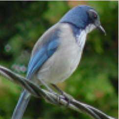
(a) Original

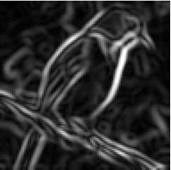
(b) Sobel

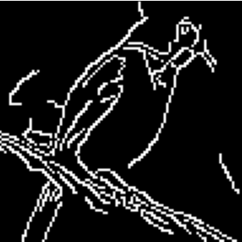
(c) Canny

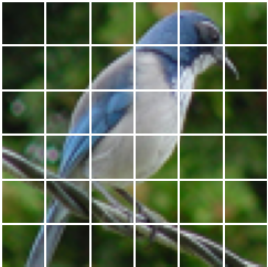
(d) BagNet

Figure 1: Visualizing different feature priors: (a) an image from the STL-10 dataset; (b) Sobel edge detection; (c) Canny edge detection; (d) the limited receptive field of a BagNet.

	CIFAR-10				STL-10
	Standard	Canny	Sobel	BagNet	Standard	Canny	Sobel	BagNet
Standard	0.598	0.237	0.259	0.38	0.554	0.305	0.385	0.357
Canny		0.545	0.324	0.143		0.523	0.392	0.212
Sobel			0.594	0.173			0.649	0.262
BagNet				0.655				0.486

Table 2: Correlation (Pearson coefficient) of correct predictions on the test set between different pairs of models. The diagonal entries correspond to models trained with the same prior but from different random initializations. While the two shape-biased models (Sobel and Canny) are more aligned with each other, they are both quite different from the texture-biased model (BagNet).

3.2 Diversity of feature-biased models

After training models with shape and texture biases as outlined above, we evaluate whether these models indeed capture complementary information about the input. Specifically, we train models on a small subset (100 examples per class) of the CIFAR-10 [Kri09] and STL-10 [CNL11] datasets, and measure the correlation between which test examples they correctly classify. We consider the full CIFAR-10 dataset, as well as similar experiments on ImageNet [DDS+09] in Appendix B.6.

We find that pairs consisting of a shape-biased model and a texture-biased model (i.e., Canny and BagNet, or Sobel and BagNet) indeed have the least correlated predictions—cf. Table 2. In other words, the mistakes that these models make are more diverse than those made by identical models trained from different random initializations. At the same time, different shape-biased models (Sobel and Canny) are relatively well-correlated with each other, which corroborates the fact that models trained on similar features of the input are likely to make similar mistakes.

Model ensembles.

Having shown that training models with these feature priors results in diverse prediction rules, we examine if we can now combine them to improve our generalization. The canonical approach for doing so is to incorporate these models into an ensemble.

We find that the diversity of models trained with different feature priors directly translates into improved performance when combining them into an ensemble—cf. Table 4. Indeed, we find that the ensemble’s performance is tightly connected to the prediction similarity of its constituents (as measured in Table 2), i.e., more diverse ensembles tend to perform better. For instance, the best ensemble for the STL-10 dataset combines a shape-biased model (Canny) and a texture-biased model (BagNet) which were the models with the least aligned predictions.

	Feature Priors	Model 1	Model 2	Ensemble
Same	Standard + Standard	52.54 $\pm$ 0.86	51.82 $\pm$ 0.86	54.02 $\pm$ 0.80
	Sobel + Sobel	51.94 $\pm$ 0.84	53.69 $\pm$ 0.82	54.68 $\pm$ 0.83
	BagNet + BagNet	42.22 $\pm$ 0.88	42.56 $\pm$ 0.80	43.49 $\pm$ 0.83
Different	Standard + Sobel	52.54 $\pm$ 0.83	51.94 $\pm$ 0.83	58.21 $\pm$ 0.82
	Standard + BagNet	52.54 $\pm$ 0.84	42.22 $\pm$ 0.84	53.03 $\pm$ 0.81
	Sobel + BagNet	51.94 $\pm$ 0.90	42.22 $\pm$ 0.84	55.14 $\pm$ 0.81

(a) CIFAR-10

	Feature Priors	Model 1	Model 2	Ensemble
Same	Standard + Standard	53.73 $\pm$ 0.91	55.38 $\pm$ 0.88	57.06 $\pm$ 0.91
	Canny + Canny	56.29 $\pm$ 0.96	54.99 $\pm$ 0.96	58.23 $\pm$ 0.93
	BagNet + BagNet	52.04 $\pm$ 0.98	50.34 $\pm$ 0.94	53.42 $\pm$ 0.93
Different	Standard + Canny	53.73 $\pm$ 0.95	56.29 $\pm$ 0.91	60.96 $\pm$ 0.96
	Standard + BagNet	53.73 $\pm$ 0.98	52.04 $\pm$ 0.90	57.17 $\pm$ 0.90
	Canny + BagNet	56.29 $\pm$ 0.91	52.04 $\pm$ 0.95	61.42 $\pm$ 0.92

(b) STL-10

Table 4: Ensemble accuracy when combining models trained with a diverse set of feature priors (models with the same prior are trained from different random initialization). Notice how models trained with different priors lead to ensembles with better performance. Moreover, when the accuracy of the two base models is comparable, models that are more diverse (as measured in Table 2) result in better ensembles. We describe the different methods of combining models in Appendix A.4 and provide the full results in Appendix B.2.

4 Combining Diverse Priors on Unlabeled Data

In the previous section, we saw that training models with different feature priors (e.g., shape- and texture-biased models) can lead to prediction rules with less overlapping failure modes—which, in turn, can lead to more effective model ensembles. However, ensembles only combine model predictions post hoc and thus cannot take advantage of diversity during the training process.

In this section, we instead focus on utilizing diversity during training. In particular, we leverage the diversity introduced through feature priors in the context of self-training [Lee+13]—a framework commonly used when the labeled data is insufficient to learn a well-generalizing model. This framework utilizes unlabeled data, which are then pseudo-labeled using an existing model and used for further training. While such methods can often improve the overall model performance, they face a significant drawback: models tend to reinforce suboptimal prediction rules even when these rules do not generalize to the underlying distribution [AOA+20].

Our goal is thus to leverage diverse feature priors to address this exact shortcoming. Specifically, we will jointly train models with different priors on the unlabeled data through the framework of co-training [BM98]. Since these models capture complementary information about the input (cf. Table 2), we expect them to correct each other’s mistakes and improve their prediction rules. As we will see in this section, this approach can indeed have a significant impact on the performance of the resulting model, outperforming ensembles that combine such models only at evaluation time—see summary in Figure 5.

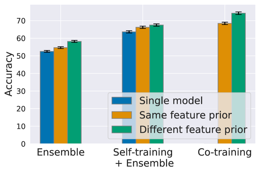
(a) CIFAR-10

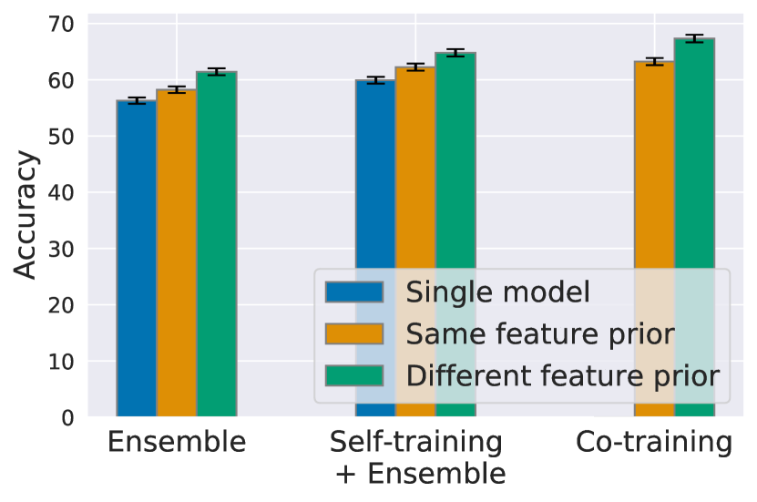
(b) STL-10

Figure 5: Test accuracy of pre-trained, self-trained, and co-trained models selecting the best feature prior for each (full results in Table 4, Appendix Table 18, and Table 7 respectively). Notice how combinations of models with different feature priors consistently outperform combinations of models with the same feature prior.

Setup.

We base our analysis on the CIFAR-10 and STL-10 datasets. Specifically, we treat a small fraction of the training set as labeled examples (100 examples per class), another fraction as our validation set for tuning hyperparameters (10% of the total training examples), and the rest as unlabeled data. We report our results on the standard test set of each dataset. (See Appendix A for experimental details, and Appendix B.7 for experiments with varying levels of labeled data.)

4.1 Self-training and ensembles

Before outlining our method for jointly training models with multiple priors, we first describe the standard approach to self-training a single model. At a high level, the predictions of the model on the unlabeled data are treated as correct labels and are then used to further train the same model [Lee+13, ITA+19, ZYL+19, XLH+20]. The underlying intuition is that the classifier will predict the correct labels for that data better than chance, and thus these pseudo-labels can be used to expand the training set.

In practice, however, these pseudo-labels tend to be noisy. Thus, a common approach is to only use the labels to which the model assigns the highest probability [Lee+13]. This process is repeated, self-training on increasingly larger fractions of the unlabeled data until all of it is used. We refer to each training phase as an era.

Ensembles of diverse self-trained models.

Similarly to our results in Table 4, we find that ensembles comprised of self-trained models with diverse feature priors outperform those using same prior from different random initializations (see Figure 5 for a summary and Appendix B.3 for the full results). This indicates that, after self-training, these models continue to capture complementary information about the input that can be leveraged to improve performance.

4.2 Co-training models with different feature priors

Moving beyond self-training with a single feature prior, our goal in this section is to leverage multiple feature priors by jointly training them on unlabeled data. This idea naturally fits into the framework of co-training: a method used to learn from unlabeled data when inputs correspond to multiple independent sets of features [BM98].

Concretely, we first train a model for each feature prior. Then, we collect the pseudo-labels on the unlabeled data that were assigned the highest probability for each model—including duplicates with potentially different labels—to form a new training set which we use for further training. As in the self-training regime, we repeat this process over several eras, increasing the fraction of the unlabeled dataset used at each era. Intuitively, this iterative process allows the models to bootstrap off of each other’s predictions, learning correlations that they might fail to learn from the labeled data alone. At the end of this process, we are left with two models, one for each prior, which we combine into a single classifier by training a standard model from scratch on the combined pseudo-labels. We provide a more detailed explanation of the methodology in Appendix A.5.

Methods	Prior(s)	Labeled Only	+Unlabeled Self/Co-Training	+ Standard model with Pseudo-labels
Self-training	Standard	52.54 $\pm$ 0.81	63.65 $\pm$ 0.78	64.02 $\pm$ 0.79
	Sobel	51.94 $\pm$ 0.90	63.05 $\pm$ 0.85	64.77 $\pm$ 0.81
	BagNet	42.22 $\pm$ 0.81	53.92 $\pm$ 0.84	54.21 $\pm$ 0.81
Co-training	Standard	52.54 $\pm$ 0.83	65.06 $\pm$ 0.78	65.10 $\pm$ 0.79
	+Standard	51.82 $\pm$ 0.79	64.93 $\pm$ 0.83
	Sobel	51.94 $\pm$ 0.82	71.88 $\pm$ 0.76	74.25 $\pm$ 0.75
	+BagNet	42.22 $\pm$ 0.80	73.91 $\pm$ 0.73

(a) CIFAR-10

Methods	Prior(s)	Labeled Only	+Unlabeled Self/Co-Training	+ Standard model with Pseudo-labels
Self-training	Standard	53.73 $\pm$ 0.94	59.92 $\pm$ 0.93	60.52 $\pm$ 0.91
	Canny	56.29 $\pm$ 0.92	58.40 $\pm$ 0.89	62.19 $\pm$ 0.91
	BagNet	52.04 $\pm$ 0.92	57.80 $\pm$ 0.99	61.69 $\pm$ 0.96
Co-training	Standard	53.73 $\pm$ 0.94	58.05 $\pm$ 0.95	61.16 $\pm$ 0.94
	+Standard	55.38 $\pm$ 0.92	60.44 $\pm$ 0.92
	Canny	56.29 $\pm$ 0.94	62.21 $\pm$ 0.93	67.33 $\pm$ 0.89
	+BagNet	52.04 $\pm$ 1.00	66.74 $\pm$ 0.94

(b) STL-10

Table 7: Test accuracy of self-training and co-training methods on STL-10 and CIFAR-10. For each model, we report the original accuracy when trained only labeled data (Column 3) as well as the accuracy after being trained on pseudo-labeled data (Column 4). (Recall that, for the case of co-training, pseudo-labeling is performed by combining the predictions of both models.) Finally, we report the performance of a standard model trained from scratch on the resulting pseudo-labels (Column 5). We provide 95% confidence intervals computed via bootstrap with 5000 iterations.

Co-training performance.

We find that co-training with shape- and texture-based priors can significantly improve test accuracy compared to self-training with any of the priors alone (Table 7). This is despite the fact that, when using self-training alone, the standard model outperforms all other models (Column 4, Table 7). Moreover, co-training models with diverse priors improves upon simply combining them in an ensemble (Appendix B.3).

In Appendix B.5, we report the performance of co-training with every pair of priors. We find that co-training with shape- and texture-based priors (Canny + BagNet for STL-10 and Sobel + BagNet for CIFAR-10) outperforms every other prior combination. Note that this differs from the setting of ensembling models with different priors, where Standard + Sobel is consistently the best performing pair for CIFAR-10 (c.f Table 4 and Appendix B.3). These results indicate that the diversity of shape- and texture-biased models allows them to improve each other over training.

Additionally, we find that, even when training a single model on the pseudo-labels of another model, prior diversity can still help. Specifically, we compare the performance of a standard model trained from scratch using pseudo-labels from various self-trained models (Column 5, Table 7). In this setting, using a self-trained shape- or texture-biased model for pseudo-labeling outperforms using a self-trained standard model. This is despite the fact that, in isolation, the standard model has higher accuracy than the shape- or texture-biased ones (Column 4, Table 7).

Model alignment over co-training.

To further explore the dynamics of co-training, we evaluate how the correlation between model predictions evolves as the eras progress in Figure 8 (using the prediction alignment measure of Table 2). We find that shape- and texture-biased models exhibit low correlation at the start of co-training, but this correlation increases as co-training progresses. This is in contrast to self-training each model on its own, where the correlation remains relatively low. It is also worth noting that the correlation appears to plateau at a lower value when co-training models with distinct feature priors as opposed to co-training two standard models.

Finally, we find that a standard model trained on the pseudo-labels of other models correlates well with the models themselves (see Appendix B.8). Overall, these findings indicate that models trained on each other’s pseudo-labels end up behaving more similarly.

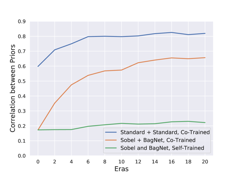
(a) CIFAR-10

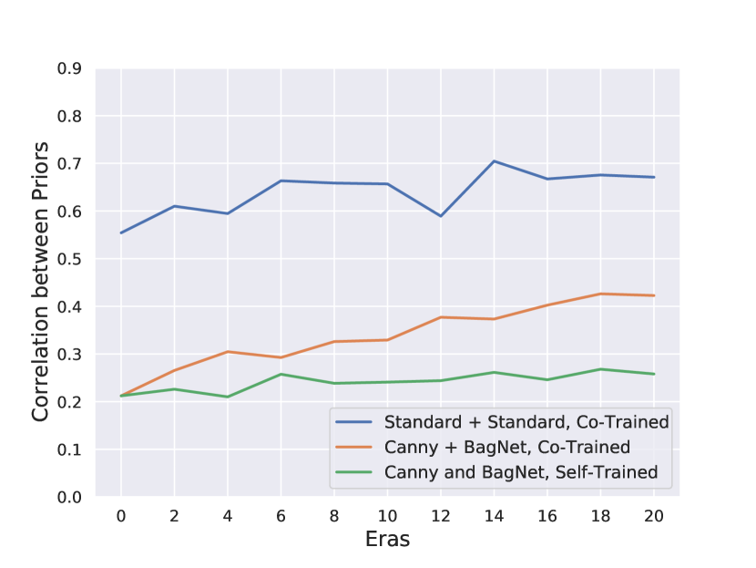
(b) STL-10

Figure 8: Correlation between the correct predictions of shape- and texture-biased models over the course of co-training for STL-10 and CIFAR-10. For comparison, we also plot the correlation between the predictions when the models induced by these priors are individually self-trained, as well as the correlation of two standard models when co-trained together.

5 Using Co-Training to Avoid Spurious Correlations

A major challenge when training models for real-world deployment is avoiding spurious correlations: associations which are predictive on the training data but not valid for the actual task. Since models are typically trained to maximize train accuracy, they are quite likely to rely on such spurious correlations [GSL+18, BVP18, GJM+20, XEI+20].

In this section, our goal is to leverage diverse feature priors to control the sensitivity of the training process to such spurious correlations. Specifically, we will assume that the spurious correlation does not hold on the unlabeled data (which is likely since unlabeled data can often be collected at a larger scale). Without this assumption, the unlabeled data contains no examples that could (potentially) contradict the spurious correlation (we investigate the setting where the unlabeled data is also similarly skewed in Appendix B.11). As we will see, if the problematic correlation is not easily captured by one of the priors, the corresponding model generates pseudo-labels that are inconsistent with this correlation, thus steering other models away from this correlation during co-training.

Setup.

We study spurious correlations in two settings. First, we create a synthetic dataset by tinting each image of the STL-10 labeled dataset in a class-specific way. The tint is highly predictive on the training set, but not on the test set (where this correlation is absent). Second, similar to [SKH+20], we consider a gender classification task based on CelebA [LLW+15] where hair color (“blond” vs. “non-blond”) is predictive on the labeled data but not on the unlabeled and test data. While gender and hair color are independent on the unlabeled dataset, the labeled dataset consists only of blond females and non-blond males. Similarly to the synthetic case, the labeled data encourages a prediction rule based only on hair color. See Appendix A.1 for details.

Methods	Prior(s)	Labeled Only	+Unlabeled Self/Co-Training	+ Standard model with Pseudo-labels
Self-training	Standard	13.99 $\pm$ 0.66	17.56 $\pm$ 0.70	17.81 $\pm$ 0.74
	Canny	55.95 $\pm$ 0.92	57.31 $\pm$ 0.89	57.81 $\pm$ 0.92
	Sobel	55.11 $\pm$ 0.91	56.12 $\pm$ 0.92	57.16 $\pm$ 0.91
	BagNet	13.10 $\pm$ 0.64	13.53 $\pm$ 0.62	14.65 $\pm$ 0.66
Co-training	Canny	55.95 $\pm$ 0.90	57.74 $\pm$ 0.90	57.85 $\pm$ 0.95
	+BagNet	13.10 $\pm$ 0.65	55.33 $\pm$ 0.92
	Sobel	55.11 $\pm$ 0.95	57.71 $\pm$ 0.90	57.60 $\pm$ 0.94
	+BagNet	13.10 $\pm$ 0.62	54.61 $\pm$ 0.94

(a) Tinted STL-10

Methods	Prior(s)	Labeled Only	+Unlabeled Self/Co-Training	+ Standard model with Pseudo-labels
Self-training	Standard	67.07 $\pm$ 0.58	71.57 $\pm$ 0.53	71.89 $\pm$ 0.53
	Canny	80.90 $\pm$ 0.47	85.73 $\pm$ 0.40	86.55 $\pm$ 0.42
	Sobel	82.94 $\pm$ 0.45	85.42 $\pm$ 0.43	84.96 $\pm$ 0.43
	BagNet	69.35 $\pm$ 0.55	64.89 $\pm$ 0.59	66.15 $\pm$ 0.58
Co-training	Canny	80.90 $\pm$ 0.46	89.64 $\pm$ 0.36	91.99 $\pm$ 0.31
	+BagNet	69.35 $\pm$ 0.55	91.44 $\pm$ 0.33
	Sobel	82.94 $\pm$ 0.44	90.64 $\pm$ 0.35	90.99 $\pm$ 0.34
	+BagNet	69.35 $\pm$ 0.57	88.72 $\pm$ 0.39

(b) CelebA

Table 10: Test accuracy of self-training and co-training on tinted STL-10 and CelebA, two datasets with spurious features (table structure is identical Table 7). In both datasets, the spurious correlation is more easily captured by the BagNet and Standard models over the shape-based ones. Nevertheless, when co-trained with a shaped-biased model, BagNets are able to significantly improve their performance, indicating that they rely less on this spurious correlation. CI: 95% bootstrap.

Performance on datasets with spurious features.

We find that, when trained only on the labeled data (where the correlation is fully predictive), both the standard and BagNet models generalize poorly in comparison to the shape-biased models (see Table 10). This behavior is expected: the spurious attribute in both datasets is color-related and mostly suppressed by the edge detection algorithms used to train shape-based models. Even after self-training on the unlabeled data (where the correlation is absent), the performance of the standard and BagNet models does not improve significantly. Finally, simply ensembling self-trained models post hoc does not improve their performance. Indeed as the texture-biased and standard models are significantly less accurate than the shape-biased one, they lower the overall accuracy of the ensemble (see Appendix B.9).

In contrast, when we co-train shape- and texture- biased models together, the texture-biased model improves substantially. When co-trained with a Canny model, the BagNet model improves over self-training by 42% on the tinted STL-10 dataset and 27% on the CelebA dataset. This improvement can be attributed to the fact that the predictions of the shape-biased model are inconsistent with the spurious correlation on the unlabeled data. By being trained on pseudo-labels from that model, the BagNet model is forced to rely on alternative, non-spurious features.

Moreover, particularly on CelebA, the shape-biased model also improves when co-trained with a texture-biased model. This indicates that even though the texture-biased model relies on the spurious correlation, it also captures non-spurious features that, during co-training, improve the performance of the shape-based model. In Appendix B.10, we find that these improvements are concentrated on inputs where the spurious correlation does not hold.

6 Additional Related Work

In Section 2, we discussed the most relevant prior work on implicit or explicit feature priors. Here, we discuss additional related work and how it connects to our approach.

Shape-biased models.

Several other methods aim to bias models towards shape-based features: input stylization [GRM+19, SMK20, LYT+21], penalizing early layer predictiveness [WGX+19], jigsaw puzzles [CDB+19, ASH+19], dropout [SZD+20], or data augmentation [HCK20]. While, in our work, we choose to suppress texture information via edge detection algorithms, any of these methods can be substituted to generate the shape-based model for our analysis.

Avoiding spurious correlations.

Other methods to avoid learning spurious correlations include: learning representations that are optimal across domains [ABG+19], enforcing robustness to group shifts [SKH+20], and utilizing multiple data points corresponding to each physical entity [HM17]. Similar in spirit to our work, these methods encourage prediction rules that are supported by multiple views of the data. However, we do not rely on annotations or multiple sources and instead impose feature priors through the model architecture and input preprocessing.

Pseudo-labeling.

Since the initial proposal of pseudo-labeling for neural networks [Lee+13], there has been a number of more sophisticated pseudo-labeling schemes aimed at improving the accuracy and diversity of the labels [ITA+19, AH20, XLH+20, RDR+21, HZZ21]. In our work, we focus on the simplest scheme for self-labeling—i.e., confidence based example selection. Nevertheless, most of these schemes can be directly incorporated into our framework to potentially improve its overall performance.

A recent line of work explores self-training by analyzing it under different assumptions on the data [MFB20, WSC+21, AL20, KML20]. Closest to our work, [CWK+20] show that self-training on unlabeled data can reduce reliance on spurious correlations under certain assumptions. In contrast, we demonstrate that by leveraging diverse feature priors, we can avoid spurious correlations even if a model heavily relies on them.

Consistency regularization.

Consistency regularization, where a model is trained to be invariant to a set of input transformations, is another canonical technique for leveraging unlabeled data. These transformations might stem from data augmentations and architecture stochasticity [LA17, BCG+19, CKN+20, SBC+20, PKK+21] or using adversarial examples [MMK+18].

Ensemble diversity.

While the standard recipe for creating model ensembles is based on training multiple identical models from different random initializations [LPB17], there do exist other methods for introducing diversity. Examples include training models with different hyperparameters [WST+20], data augmentations [SM20], input transformations [YKZ21], or model architectures [ZZE+20]. Note that, in contrast to our work, none of these approaches incorporate this diversity into training itself.

Co-training.

One line of work studies co-training from a theoretical perspective [NG00, BBY05, GZ00]. Other work aims to improve co-training by either expanding the settings where it can be applied [CWC11] or by improving its stability [MMD+20, ZZ11]. Finally, a third line of work applies co-training to images. Since images cannot be separated into disjoint feature sets, one applies co-training by training multiple models [HYY+18], either regularized to be diverse through adversarial examples [QSZ+18] or trained using different methods [YWG+20]. Our method is complementary to these approaches as it relies on explicit feature priors to obtain different views.

7 Conclusion

In this work, we explored the benefits of combining feature priors with non-overlapping failure modes. By capturing complementary perspectives on the data, models trained with diverse feature priors can offset each other’s mistakes when combined through methods such as ensembles. Moreover, in the presence of unlabeled data, we can leverage prior diversity by jointly boostrapping models with different priors through co-training. This allows the models to correct each other during training, thus improving pseudo-labeling and controlling for correlations that do not generalize well.

We believe that our work is only the first step in exploring the design space of creating, manipulating, and combining feature priors to improve generalization. In particular, our framework is quite flexible and allows for a number of different design choices, such as choosing other feature priors (cf. Sections 2 and 6), using other methods for pseudo-label selection (e.g., using uncertainty estimation [LLL+18, RDR+21]), and combining pseudo-labels via different ensembling methods. More broadly, we believe that exploring the synthesis of explicit feature priors in new applications is an exciting avenue for further research.

Appendix A Experimental Details

A.1 Datasets

For our first set of experiments (Section 4), we focus on a canonical setting where a small portion of the training set if labeled and we have access to a pool of unlabeled data.

STL-10.

The STL-10 [CNL11] dataset contains 5,000 training and 8,000 test images of size 96$\times$96 from 10 classes. We designate 1,000 of the 5,000 (20%) training examples to be the labeled training set, 500 (10%) to be the validation set, and the rest are used as unlabeled data.

CIFAR-10.

The CIFAR-10 [Kri09] dataset contains 50,000 training and 8,000 test images of size 32$\times$32 from 10 classes. We designate 1,000 of the 50,000 (2%) training examples to be the labeled training set, 5000 (10%) to be the validation set, and the rest as unlabeled data.

In both cases, we report the final performance on the standard test set of that dataset. We also create two datasets that each contain a different spurious correlation.

Tinted STL-10.

We reuse the STL-10 setup described above, but we add a class-specific tint to each image in the (labeled) training set. Specifically, we hand-pick a different color for each of the 10 classes and then add this color to each of the pixels (ensuring that each RGB channel remains within the valid range)—see Figure 11 for examples. This tint is only present in the labeled part of the training set, the unlabeled and test parts of the dataset are left unaltered.

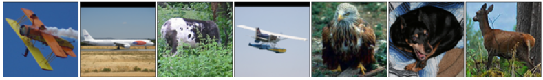
(a) Original

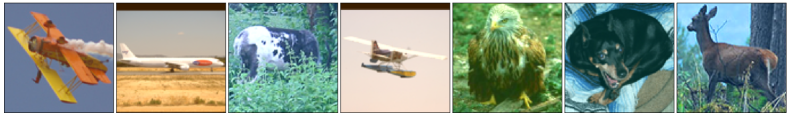
(b) Tinted

Figure 11: Tinted STL-10 images. The tint is class-specific and thus models can learn to predict based mostly on that tint.

Biased CelebA.

We consider the task of predicting gender in the CelebA [LLW+15] dataset. In order to create a biased training set, we choose a random sample of 500 non-blond males and 500 blond females. We then use a balanced unlabeled dataset consisting of 1,000 random samples for each of: blond males, blond females, non-blond males, and non-blond females. We use the standard CelebA test set which consists of 12.41% blond females, 48.92% non-blond females, 0.90% blond males, and 37.77% non-blond males. (Note that a classifier predicting purely based on hair color with have an accuracy of 50.18% on that test set.)

All of the datasets that we use are freely available for non-commercial research purposes. Moreover, to the best of our knowledge, they do not contain offensive content or identifiable information (other than publicly available celebrity photos).

A.2 Model architectures and input preprocessing

For both the standard model and the models trained on images processed by edge detection algorithm, we use a standard model architecture—namely, VGG16 [SZ15] with the addition of batch normalization [IS15] (often referred to as VGG16-BN). We describe the exact edge detection process as well as the architecture of the BagNet model (texture prior) below. We visualize these priors in Figure 13.

Canny edge detection.

Given an image, we first smooth it with a 5 pixel bilateral filter [TM98], with filter $\sigma$ in the coordinate and color space set to 75. After smoothing, the image is converted to gray-scale. Finally, a Canny filter [Can86] is applied to the image, with hysteresis thresholds 100 and 200, to extract the edges.

Sobel edge detection.

Given an image, we first upsample it to 128$\times$128 pixels. Then we convert it to gray-scale and apply a Gaussian blur (kernel size=5, $\sigma=5$). The image is then passed through a Sobel filter [SF68] with a kernel size of 3 in both the horizontal and the vertical direction to extract the image gradients.

BagNet.

For our texture-biased model, we use a slimmed down version of the BagNet architecture from [BB19]. The goal of this architecture is to limit the receptive field of the model, hence forcing it to make predictions based on local features. The exact architecture we used is shown in Figure 12. Intuitively, the top half of the network—i.e., the green and blue blocks—construct features on patches of size 20$\times$20 for 96$\times$96 images and 10$\times$10 for 32$\times$32 images. The rest of the network consists only of 1$\times$1 convolutions and max-pooling, hence not utilizing the image’s spatial structure.

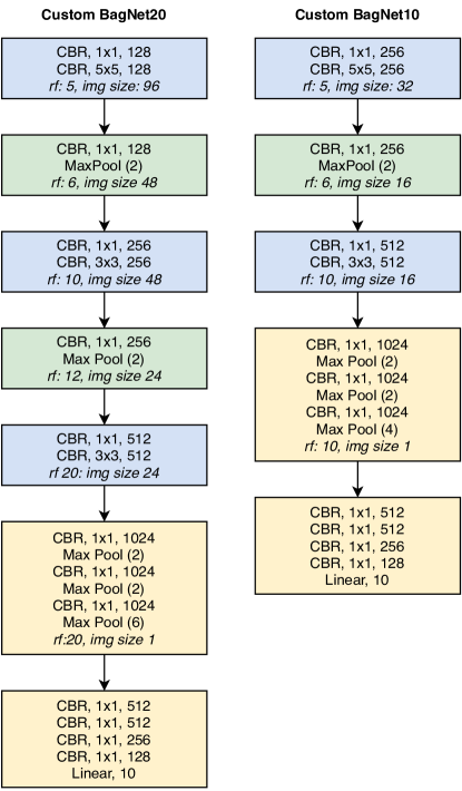
Figure 12: The customized BagNet architecture used for training texture-biased models. The basic building block consists of a convolutional layer, followed by batch normalization and finally a ReLU non-linearity (denoted collectively as CBR).

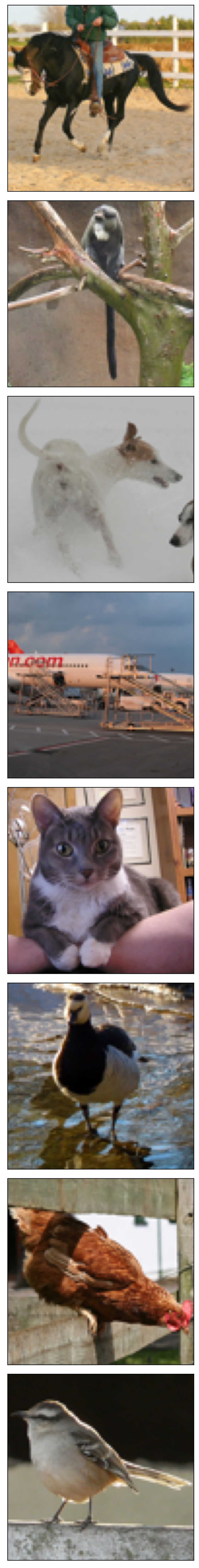
(a) Original

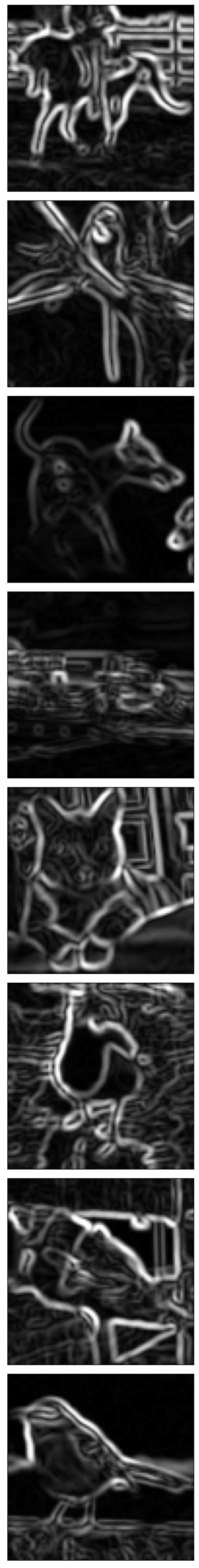
(b) Sobel

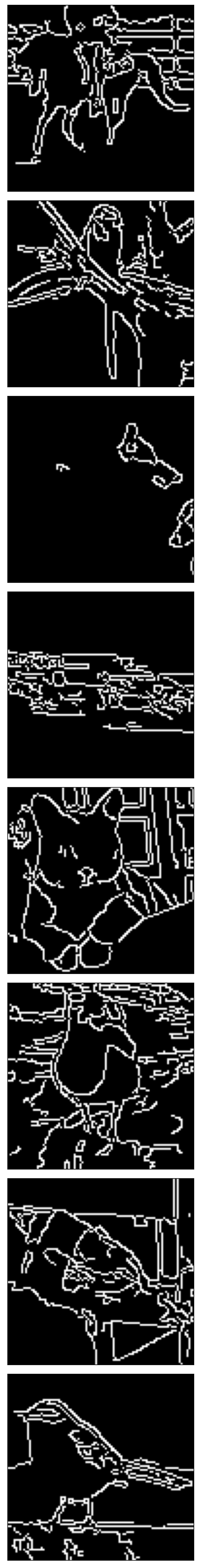
(c) Canny

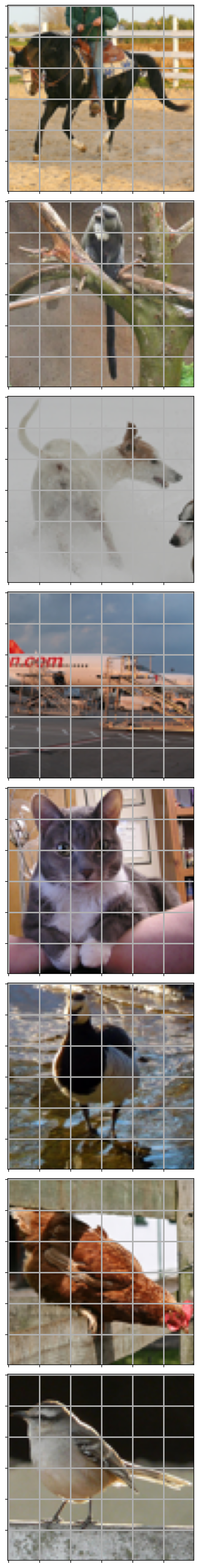
(d) BagNet

Figure 13: Further visualizations of the different feature priors we introduce. For each original image (a), we visualize the output of both edge detection algorithms—Sobel (b) and Canny (c)—as well as the receptive field of the BagNet model.

A.3 Training setup

A.3.1 Basic training

We train all our models using stochastic gradient descent (SGD) with momentum (a coefficient of 0.9) and a decaying learning rate. We add weight decay regularization with a coefficient of $10^{-4}$. In terms of data augmentation, we apply random cropping with a padding of 4 pixels, random horizontal flips, and a random rotation of $\pm 2$ degrees. These transformations are applied after the edge detection processing. We train all models with a batch size of 64 for 96$\times$96-sized images and 128 for 32$\times$32-sized images for a total of 300 epochs. All our experiments are performed using our internal cluster which mainly consists of NVIDIA 1080 Ti GTX GPUs.

Hyperparameter tuning.

To ensure a fair comparison across feature priors, we selected the hyperparameters for each dataset-prior pair separately, using the held-out validation set (separate from the final test used for reporting performance). Specifically, we performed a grid search choosing the learning rate (LR) from $[0.1,0.05,0.02,0.01,0.005]$, the number of epochs between each learning rate drop ($K$) from $[50,100,300]$ and the factor with which the learning rate is multiplied ($\gamma$) from $[0.5,1]$. The parameters chosen are shown in Table 14. We found that all models achieved near-optimal performance strictly within the range of each hyperparameters. Thus, we did not consider a wider grid.

Dataset	Prior	LR	$\gamma$	$K$
STL-10	Standard	0.01	0.5	100
	Canny	0.01	0.5	100
	Sobel	0.005	0.5	100
	BagNet	0.05	0.5	100
CIFAR-10	Standard	0.01	0.5	100
	Canny	0.01	0.5	100
	Sobel	0.01	0.5	100
	BagNet	0.01	0.1	100
CelebA	Standard	0.005	0.5	50
	Canny	0.005	0.1	100
	Sobel	0.01	0.5	50
	BagNet	0.02	0.5	100

Table 14: Hyperparameters chosen through grid search for each dataset-prior pair (we used the STL-10 hyperparameters for the tinted STL-10 dataset). LR corresponds to the learning rate, $\gamma$ to the factor used to decay the learning rate at each drop, and $K$ to the train epochs between each learning rate drop.

A.4 Ensembles

In order to leverage prior diversity, we ensemble models trained with (potentially) different priors. We use the following ensembles:

1. Take Max: Predict based on the model assigning the highest probability on this example.

2. Average: Average the (softmax) output probabilities of the models, predict the class assigned the highest probability.

3. Rank: Each model ranks all test examples based on the probability assigned to their predicted labels. Then, for each example, we predict using the model which has a lower rank on this example.

We then report the maximum of these ensemble methods in Table 4. We separately examine a more complex ensembling method (stacked ensembling) in Appendix B.4.

A.5 Self-training and co-training schemes

In the setting that we are focusing on, we are provided with a labeled dataset $\mathbf{X}$ and an unlabeled dataset $\mathbf{U}$, where typically there is much more unlabeled data ($|\mathbf{U}|\gg|\mathbf{X}|$). We are then choosing a set of (one or more) feature priors each of which corresponds to a different way of training a model (e.g., using edge detection preprocessing).

General methodology.

We start by training each of these models on the labeled dataset. Then, we combine the predictions of these models to produce pseudo-labels for the unlabeled dataset. Finally, we choose a fraction of the unlabeled data and train the models on that set using the produced pseudo-labels (in additional to the original labeled set $X$). This process is repeated using increasing fractions of the unlabeled dataset until, eventually, models are trained on its entirety. We refer to each such phase as an era. We include an additional 5% of the unlabeled data per era, resulting in a total of 20 eras. During each era, we use the training process described in Appendix A.3.1 without re-initializing the models (warm start). After completing this process, we train a standard model from scratch using both the labeled set and resulting pseudo-labels. The methodology used for choosing and combining pseudo-labels is described below for each scheme.

Self-training.

Since we are only training one model, we only need to decide how to choose the pseudo-labels to use for each era. We do this in the simplest way: at ear $t$, we pick the subset $\mathbf{U_{t}}\subseteq\mathbf{U}$ of examples that are assigned the highest probability on their predicted label. We attempt to produce a class-balanced training set by applying this process separately on each class (as predicted by the model). The pseudocode for the method is provided in Algorithm 1.

Parameters : Number of eras $T$. Fraction added per era $k$.

Input : Labeled data $\mathbf{X}$ with $n$ classes, unlabeled data $\mathbf{U}$, model trained on $\mathbf{X}$.

for era $t\in 1...T$ do

       forward-pass $\mathbf{U}$ through the model to create pseudo-labels

       $\mathbf{U_{t}}=[]$

       for each class $c$  do

             Select the $\frac{kt|\mathbf{U}|}{n}$ most confident examples from $\mathbf{U}$ predicted by the model as class $c$

             Add those examples to $\mathbf{U_{t}}$ with class $c$

            

      Re-train (warm start) the model on $\mathbf{X}\cup\mathbf{U_{t}}$ until convergence

      

Train a standard model from scratch on $\mathbf{X}\cup\mathbf{U_{T}}$.

Algorithm 1 Self-training

Standard co-training.

Here, we train multiple models (in our experiments two) based on a common pool of pseudo-labeled examples in each era. In each era $t$, each model labels the unlabeled dataset $\mathbf{U}$. Then, for each class, we alternate between models, adding the next most confident example predicted as that class for that model to $\mathbf{U_{t}}$, until we reach a fixed number of unique examples have been added for that class (5% of the size of the unlabeled dataset per era). Note that this process allows both conflicts and duplicates: if multiple models are confident about a specific example, that example may be added more than once (potentially with a different label each time). Finally, we train each model (without re-initializing) on $\mathbf{X}\cup\mathbf{U_{t}}$. The pseudocode for this method can be found in Algorithm 2.

Parameters : Number of eras $T$. Fraction added per era $k$.

Input : Labeled data $\mathbf{X}$ with $n$ classes, unlabeled data $\mathbf{U}$, models trained on $\mathbf{X}$.

for era $t\in 1...T$ do

       forward-pass $\mathbf{U}$ through each model to create pseudo-labels

       $\mathbf{U_{t}}=[]$

       for each class $c$ do

             $\mathbf{U_{t}^{(c)}}=[]$

             while the number of unique examples in $\mathbf{U_{t}^{(c)}}<\frac{kt|\mathbf{U}|}{n}$ do

                   for each model $m$ do

                         Add the next most confident example predicted by $m$ as class $c$ to $\mathbf{U_{t}^{(c)}}$

                        

                  

            Add $\mathbf{U_{t}^{(c)}}$ to $\mathbf{U_{t}}$

      Re-train (warm start) each model on $\mathbf{X}\cup\mathbf{U_{t}}$ until convergence

      

Train a standard model from scratch on $\mathbf{X}\cup\mathbf{U_{T}}$.

Algorithm 2 Standard Co-Training

Appendix B Additional Experiments

B.1 Experiment organization

We now provide the full experimental results used to create the plots in the main body as well as additional analysis. Specifically, in Appendix B.2 and B.3 we present the performance of individual ensemble schemes for pre-trained and self-trained models respectively. Then, in Appendix B.5 we present the performance of co-training for each combination of feature priors. In Appendix B.8 we analyse the effect that co-training has on model similarity after training. Finally, in Appendix B.9 we evaluate model ensembles on datasets with spurious correlations and in Appendix B.10 we breakdown the performance of co-training on the skewed CelebA dataset according to different input attributes.

B.2 Full Pre-Trained Ensemble Results

In Table 4, we reported the best ensemble method for each pair of models trained with different priors on the labeled data. In Table 16, we report the full results over the individual ensembles.

Feature Priors	Model 1	Model 2	Max Conf.	Avg Conf.	Rank	Best
Standard + Standard	52.54 $\pm$ 0.85	51.82 $\pm$ 0.85	53.98 $\pm$ 0.83	54.02 $\pm$ 0.85	53.98 $\pm$ 0.83	54.02 $\pm$ 0.82
Sobel + Sobel	51.94 $\pm$ 0.88	53.69 $\pm$ 0.86	54.62 $\pm$ 0.83	54.68 $\pm$ 0.86	54.61 $\pm$ 0.85	54.68 $\pm$ 0.83
Canny + Canny	45.48 $\pm$ 0.84	44.19 $\pm$ 0.88	46.46 $\pm$ 0.82	46.48 $\pm$ 0.86	46.70 $\pm$ 0.83	46.70 $\pm$ 0.79
BagNet + BagNet	42.22 $\pm$ 0.80	42.56 $\pm$ 0.83	43.32 $\pm$ 0.82	43.49 $\pm$ 0.82	43.33 $\pm$ 0.85	43.49 $\pm$ 0.84
Standard + Sobel	52.54 $\pm$ 0.79	51.94 $\pm$ 0.82	58.14 $\pm$ 0.82	58.21 $\pm$ 0.88	58.12 $\pm$ 0.82	58.21 $\pm$ 0.90
Standard + Canny	52.54 $\pm$ 0.87	45.48 $\pm$ 0.81	55.18 $\pm$ 0.82	55.49 $\pm$ 0.83	54.41 $\pm$ 0.81	55.49 $\pm$ 0.83
Standard + BagNet	52.54 $\pm$ 0.85	42.22 $\pm$ 0.80	52.89 $\pm$ 0.84	53.03 $\pm$ 0.89	50.69 $\pm$ 0.81	53.03 $\pm$ 0.85
Sobel + Canny	51.94 $\pm$ 0.82	45.48 $\pm$ 0.85	53.81 $\pm$ 0.84	53.95 $\pm$ 0.80	53.18 $\pm$ 0.91	53.95 $\pm$ 0.85
Sobel + BagNet	51.94 $\pm$ 0.86	42.22 $\pm$ 0.82	54.42 $\pm$ 0.84	55.14 $\pm$ 0.83	53.50 $\pm$ 0.82	55.14 $\pm$ 0.84
Canny + BagNet	45.48 $\pm$ 0.78	42.22 $\pm$ 0.79	49.95 $\pm$ 0.84	50.57 $\pm$ 0.82	49.64 $\pm$ 0.81	50.57 $\pm$ 0.84

(a) Ensemble Baselines for CIFAR-10

Feature Priors	Model 1	Model 2	Max Conf.	Avg Conf.	Rank	Best
Standard + Standard	53.73 $\pm$ 0.86	55.38 $\pm$ 1.00	56.95 $\pm$ 0.94	57.06 $\pm$ 0.91	56.94 $\pm$ 0.97	57.06 $\pm$ 0.91
Sobel + Sobel	55.49 $\pm$ 0.94	55.64 $\pm$ 0.98	56.71 $\pm$ 0.92	56.83 $\pm$ 0.90	56.66 $\pm$ 0.89	56.83 $\pm$ 0.94
Canny + Canny	56.29 $\pm$ 0.92	54.99 $\pm$ 0.96	58.04 $\pm$ 0.94	58.23 $\pm$ 0.94	57.95 $\pm$ 0.89	58.23 $\pm$ 0.93
BagNet + BagNet	52.04 $\pm$ 0.92	50.34 $\pm$ 0.90	53.40 $\pm$ 0.98	53.42 $\pm$ 0.91	53.29 $\pm$ 0.96	53.42 $\pm$ 0.98
Standard + Sobel	53.73 $\pm$ 0.94	55.49 $\pm$ 0.95	59.01 $\pm$ 0.90	59.08 $\pm$ 0.91	58.94 $\pm$ 0.96	59.08 $\pm$ 0.95
Standard + Canny	53.73 $\pm$ 1.00	56.29 $\pm$ 0.94	60.90 $\pm$ 0.94	60.96 $\pm$ 0.94	60.85 $\pm$ 0.87	60.96 $\pm$ 0.94
Standard + BagNet	53.73 $\pm$ 0.95	52.04 $\pm$ 0.90	56.99 $\pm$ 0.94	57.17 $\pm$ 0.92	57.04 $\pm$ 0.91	57.17 $\pm$ 0.94
Sobel + Canny	55.49 $\pm$ 0.91	56.29 $\pm$ 0.94	59.92 $\pm$ 0.95	60.02 $\pm$ 0.97	59.77 $\pm$ 0.91	60.02 $\pm$ 0.91
Sobel + BagNet	55.49 $\pm$ 0.94	52.04 $\pm$ 0.95	59.17 $\pm$ 0.94	59.76 $\pm$ 0.96	59.08 $\pm$ 0.89	59.76 $\pm$ 0.87
Canny + BagNet	56.29 $\pm$ 0.96	52.04 $\pm$ 0.95	61.09 $\pm$ 0.92	61.42 $\pm$ 0.94	60.68 $\pm$ 0.92	61.42 $\pm$ 0.93

(b) Ensemble Baselines for STL-10

Table 16: Full results for ensembles of pre-trained models.

B.3 Ensembling Self-Trained Models

In Table 18, we report the best ensemble method for pairs of self-trained models with different priors. In Table 20, we report the full results over the individual ensembles. We find that, similar to the ensembles of models trained on the labeled data, models with diverse priors gain more from ensembling. However, co-training models with diverse priors together still outperforms ensembling self-trained models.

	Feature Priors	Model 1	Model 2	Ensemble
Same	Standard + Standard	59.92 $\pm$ 0.95	59.34 $\pm$ 0.88	62.25 $\pm$ 0.93
	Canny + Canny	58.40 $\pm$ 0.94	57.69 $\pm$ 0.94	60.38 $\pm$ 0.92
	BagNet + BagNet	57.80 $\pm$ 0.96	58.11 $\pm$ 0.85	60.52 $\pm$ 0.90
Different	Standard + Canny	59.92 $\pm$ 0.90	58.40 $\pm$ 0.95	64.44 $\pm$ 0.90
	Standard + BagNet	59.92 $\pm$ 0.94	57.80 $\pm$ 0.96	63.19 $\pm$ 0.87
	Canny + BagNet	58.40 $\pm$ 0.94	57.80 $\pm$ 0.96	64.80 $\pm$ 0.91

(a) STL-10

	Feature Priors	Model 1	Model 2	Ensemble
Same	Standard + Standard	63.65 $\pm$ 0.81	61.95 $\pm$ 0.82	64.85 $\pm$ 0.79
	Sobel + Sobel	63.05 $\pm$ 0.81	66.01 $\pm$ 0.80	66.25 $\pm$ 0.82
	BagNet + BagNet	53.92 $\pm$ 0.82	52.90 $\pm$ 0.91	55.00 $\pm$ 0.83
Different	Standard + Sobel	63.65 $\pm$ 0.81	63.05 $\pm$ 0.83	67.52 $\pm$ 0.77
	Standard + BagNet	63.65 $\pm$ 0.81	53.92 $\pm$ 0.88	64.10 $\pm$ 0.79
	Sobel + BagNet	63.05 $\pm$ 0.83	53.92 $\pm$ 0.89	65.68 $\pm$ 0.79

(b) CIFAR-10

Table 18: Ensemble performance when combining self-trained models with Standard, Canny, Sobel, and BagNet priors. When two models of the same prior are ensembled, the models are trained with different random initializations.

Feature Priors	Model 1	Model 2	Max Conf.	Avg Conf.	Rank	Best
Standard + Standard	63.65 $\pm$ 0.81	61.95 $\pm$ 0.87	64.84 $\pm$ 0.77	64.85 $\pm$ 0.76	64.83 $\pm$ 0.83	64.85 $\pm$ 0.79
Sobel + Sobel	63.05 $\pm$ 0.87	66.01 $\pm$ 0.82	66.19 $\pm$ 0.81	66.25 $\pm$ 0.79	66.17 $\pm$ 0.81	66.25 $\pm$ 0.83
BagNet + BagNet	53.92 $\pm$ 0.87	52.90 $\pm$ 0.83	54.86 $\pm$ 0.87	55.00 $\pm$ 0.83	54.87 $\pm$ 0.82	55.00 $\pm$ 0.87
Standard + Sobel	63.65 $\pm$ 0.79	63.05 $\pm$ 0.80	67.42 $\pm$ 0.79	67.52 $\pm$ 0.79	67.38 $\pm$ 0.79	67.52 $\pm$ 0.77
Standard + Canny	63.65 $\pm$ 0.90	51.82 $\pm$ 0.88	63.70 $\pm$ 0.81	63.91 $\pm$ 0.81	63.02 $\pm$ 0.83	63.91 $\pm$ 0.82
Standard + BagNet	63.65 $\pm$ 0.81	53.92 $\pm$ 0.82	64.05 $\pm$ 0.85	64.10 $\pm$ 0.79	62.69 $\pm$ 0.80	64.10 $\pm$ 0.86
Sobel + Canny	63.05 $\pm$ 0.81	51.82 $\pm$ 0.80	61.43 $\pm$ 0.80	61.42 $\pm$ 0.80	60.66 $\pm$ 0.81	61.43 $\pm$ 0.83
Sobel + BagNet	63.05 $\pm$ 0.78	53.92 $\pm$ 0.83	65.45 $\pm$ 0.85	65.68 $\pm$ 0.82	64.65 $\pm$ 0.80	65.68 $\pm$ 0.82
Canny + BagNet	51.82 $\pm$ 0.81	53.92 $\pm$ 0.79	59.60 $\pm$ 0.81	59.79 $\pm$ 0.83	60.24 $\pm$ 0.82	60.24 $\pm$ 0.81

(a) Ensemble Baselines for CIFAR-10

Feature Priors	Model 1	Model 2	Max Conf.	Avg Conf.	Rank	Best
Standard + Standard	59.92 $\pm$ 0.92	59.34 $\pm$ 0.99	62.18 $\pm$ 0.92	62.25 $\pm$ 0.96	62.16 $\pm$ 0.88	62.25 $\pm$ 0.94
Canny + Canny	58.40 $\pm$ 0.95	57.69 $\pm$ 0.89	60.30 $\pm$ 0.95	60.36 $\pm$ 0.92	60.38 $\pm$ 0.91	60.38 $\pm$ 0.95
BagNet + BagNet	57.80 $\pm$ 0.89	58.11 $\pm$ 0.94	60.42 $\pm$ 0.90	60.46 $\pm$ 0.98	60.52 $\pm$ 0.93	60.52 $\pm$ 0.90
Standard + Sobel	59.92 $\pm$ 0.92	57.86 $\pm$ 0.91	62.49 $\pm$ 0.89	62.69 $\pm$ 0.91	62.66 $\pm$ 0.89	62.69 $\pm$ 0.94
Standard + Canny	59.92 $\pm$ 0.94	58.40 $\pm$ 0.95	64.29 $\pm$ 0.95	64.44 $\pm$ 0.89	64.34 $\pm$ 0.95	64.44 $\pm$ 0.95
Standard + BagNet	59.92 $\pm$ 0.89	57.80 $\pm$ 0.97	63.01 $\pm$ 0.93	63.10 $\pm$ 0.89	63.19 $\pm$ 0.88	63.19 $\pm$ 0.88
Sobel + Canny	57.86 $\pm$ 0.91	58.40 $\pm$ 0.93	62.20 $\pm$ 0.92	62.14 $\pm$ 0.92	62.22 $\pm$ 0.90	62.22 $\pm$ 0.91
Sobel + BagNet	57.86 $\pm$ 0.95	57.80 $\pm$ 0.95	62.24 $\pm$ 0.94	62.58 $\pm$ 0.90	63.52 $\pm$ 0.91	63.52 $\pm$ 0.88
Canny + BagNet	58.40 $\pm$ 0.93	57.80 $\pm$ 0.95	64.38 $\pm$ 0.89	64.64 $\pm$ 0.92	64.80 $\pm$ 0.90	64.80 $\pm$ 0.92

(b) Ensemble Baselines for STL-10

Table 20: Full results for ensembles of self-trained models.

B.4 Stacked Ensembling

Here we consider an ensembling technique that leverages a validation set. We implement stacking (also called blending) [TJB09, STM+09], which takes in the outputs of the member models as input, and then trains a second model to produce the final layer. Here, we take the logits of each model in the ensemble, and train the secondary model using logistic regression on the validation set for the dataset. We report accuracies of the ensemble on the test set below. We again find that prior diversity is important for the performance of the ensemble.

	Pre-trained			Self-trained
Feature Priors	Model 1	Model 2	Stacked Ensemble	Model 1	Model 2	Stacked Ensemble
Standard + Standard	52.54 $\pm$ 0.85	51.82 $\pm$ 0.85	54.13 $\pm$ 0.88	63.65 $\pm$ 0.81	61.95 $\pm$ 0.82	65.13 $\pm$ 0.82
Sobel + Sobel	51.94 $\pm$ 0.88	53.69 $\pm$ 0.86	54.46 $\pm$ 0.92	63.05 $\pm$ 0.81	66.01 $\pm$ 0.80	66.35 $\pm$ 0.80
BagNet + BagNet	42.22 $\pm$ 0.80	42.56 $\pm$ 0.83	44.28 $\pm$ 0.83	53.92 $\pm$ 0.82	52.90 $\pm$ 0.91	54.94 $\pm$ 0.84
Standard + Sobel	52.54 $\pm$ 0.79	51.94 $\pm$ 0.82	57.42 $\pm$ 0.84	63.65 $\pm$ 0.81	63.05 $\pm$ 0.83	67.01 $\pm$ 0.79
Standard + BagNet	52.54 $\pm$ 0.85	42.22 $\pm$ 0.80	53.65 $\pm$ 0.85	63.65 $\pm$ 0.81	53.92 $\pm$ 0.88	64.61 $\pm$ 0.81
Sobel + BagNet	51.94 $\pm$ 0.86	42.22 $\pm$ 0.82	55.75 $\pm$ 0.83	63.05 $\pm$ 0.83	53.92 $\pm$ 0.89	65.67 $\pm$ 0.82

Table 21: Performance of ensembling pre-trained and self-trained models with stacked ensembling on CIFAR-10.

	Pre-trained			Self-trained
Feature Priors	Model 1	Model 2	Stacked Ensemble	Model 1	Model 2	Stacked Ensemble
Standard + Standard	53.73 $\pm$ 0.86	55.38 $\pm$ 1.00	56.01 $\pm$ 0.94	59.92 $\pm$ 0.95	59.34 $\pm$ 0.88	60.54 $\pm$ 0.91
Canny + Canny	56.29 $\pm$ 0.92	54.99 $\pm$ 0.96	57.70 $\pm$ 0.90	58.40 $\pm$ 0.94	57.69 $\pm$ 0.94	59.23 $\pm$ 0.99
BagNet + BagNet	52.04 $\pm$ 0.92	50.34 $\pm$ 0.90	52.35 $\pm$ 0.97	57.80 $\pm$ 0.96	58.11 $\pm$ 0.85	59.48 $\pm$ 0.98
Standard + Canny	53.73 $\pm$ 1.00	56.29 $\pm$ 0.94	59.24 $\pm$ 0.88	59.92 $\pm$ 0.90	58.40 $\pm$ 0.95	63.42 $\pm$ 0.89
Standard + BagNet	53.73 $\pm$ 0.95	52.04 $\pm$ 0.90	56.03 $\pm$ 0.98	59.92 $\pm$ 0.94	57.80 $\pm$ 0.96	62.59 $\pm$ 0.91
Canny + BagNet	56.29 $\pm$ 0.96	52.04 $\pm$ 0.95	59.98 $\pm$ 0.91	58.40 $\pm$ 0.94	57.80 $\pm$ 0.96	63.22 $\pm$ 0.94

Table 22: Performance of ensembling pre-trained and self-trained models with stacked ensembling on STL-10.

B.5 Self-Training and Co-Training on STL-10 and CIFAR-10

Methods	Prior(s)	Labeled Only	+Unlabeled Self/Co-Training	+ Standard model with Pseudo-labels
Self-training	Standard	52.54 $\pm$ 0.86	63.65 $\pm$ 0.76	64.02 $\pm$ 0.82
	Canny	45.48 $\pm$ 0.90	51.82 $\pm$ 0.82	55.59 $\pm$ 0.80
	Sobel	51.94 $\pm$ 0.88	63.05 $\pm$ 0.84	64.77 $\pm$ 0.80
	BagNet	42.22 $\pm$ 0.82	53.92 $\pm$ 0.89	54.21 $\pm$ 0.85
Co-training	Standard	52.54 $\pm$ 0.91	65.06 $\pm$ 0.76	65.10 $\pm$ 0.84
	+Standard	51.82 $\pm$ 0.86	64.93 $\pm$ 0.80
	Canny	45.48 $\pm$ 0.85	51.15 $\pm$ 0.79	55.74 $\pm$ 0.80
	+Canny	44.19 $\pm$ 0.82	51.65 $\pm$ 0.81
	Sobel	51.94 $\pm$ 0.86	67.18 $\pm$ 0.80	68.47 $\pm$ 0.74
	+Sobel	53.69 $\pm$ 0.89	67.35 $\pm$ 0.77
	Canny	45.48 $\pm$ 0.79	58.66 $\pm$ 0.81	65.34 $\pm$ 0.81
	+Sobel	51.94 $\pm$ 0.80	64.87 $\pm$ 0.79
	Canny	45.48 $\pm$ 0.85	59.19 $\pm$ 0.85	67.59 $\pm$ 0.74
	+BagNet	42.22 $\pm$ 0.85	67.92 $\pm$ 0.79
	Sobel	51.94 $\pm$ 0.81	71.88 $\pm$ 0.73	74.25 $\pm$ 0.74
	+BagNet	42.22 $\pm$ 0.82	73.91 $\pm$ 0.71
	BagNet	42.22 $\pm$ 0.79	55.94 $\pm$ 0.83	56.05 $\pm$ 0.77
	+BagNet	42.56 $\pm$ 0.86	55.26 $\pm$ 0.88
	Canny	45.48 $\pm$ 0.85	59.23 $\pm$ 0.81	67.21 $\pm$ 0.77
	+Standard	52.54 $\pm$ 0.87	66.92 $\pm$ 0.82
	Sobel	51.94 $\pm$ 0.83	71.44 $\pm$ 0.76	73.83 $\pm$ 0.76
	+Standard	52.54 $\pm$ 0.85	73.59 $\pm$ 0.72
	Standard	52.54 $\pm$ 0.88	66.67 $\pm$ 0.83	66.77 $\pm$ 0.75
	+BagNet	42.22 $\pm$ 0.80	67.12 $\pm$ 0.75

Table 23: Performance of self-training and co-training on CIFAR-10 for each prior combination.

Methods	Prior(s)	Labeled Only	+Unlabeled Self/Co-Training	+ Standard model with Pseudo-labels
Self-training	Standard	53.73 $\pm$ 0.95	59.92 $\pm$ 0.91	60.52 $\pm$ 0.94
	Canny	56.29 $\pm$ 0.96	58.40 $\pm$ 0.91	62.19 $\pm$ 0.92
	Sobel	55.49 $\pm$ 0.96	57.86 $\pm$ 0.98	60.92 $\pm$ 0.89
	BagNet	52.04 $\pm$ 0.96	57.80 $\pm$ 0.99	61.69 $\pm$ 0.95
Co-training	Standard	53.73 $\pm$ 0.95	58.05 $\pm$ 0.92	61.16 $\pm$ 0.95
	+Standard	55.38 $\pm$ 0.96	60.44 $\pm$ 0.95
	Canny	56.29 $\pm$ 0.92	60.22 $\pm$ 0.91	63.24 $\pm$ 0.92
	+Canny	54.99 $\pm$ 0.94	59.56 $\pm$ 0.94
	Sobel	55.49 $\pm$ 0.96	58.93 $\pm$ 0.91	60.68 $\pm$ 0.94
	+Sobel	55.64 $\pm$ 0.95	59.23 $\pm$ 0.90
	Canny	56.29 $\pm$ 0.95	62.40 $\pm$ 0.99	65.53 $\pm$ 0.84
	+Sobel	55.49 $\pm$ 0.92	64.11 $\pm$ 0.91
	Canny	56.29 $\pm$ 0.92	62.21 $\pm$ 0.89	67.33 $\pm$ 0.88
	+BagNet	52.04 $\pm$ 0.94	66.74 $\pm$ 0.87
	Sobel	55.49 $\pm$ 0.92	62.72 $\pm$ 0.94	65.79 $\pm$ 0.94
	+BagNet	52.04 $\pm$ 1.00	65.44 $\pm$ 0.91
	BagNet	52.04 $\pm$ 0.89	59.85 $\pm$ 0.89	60.84 $\pm$ 0.95
	+BagNet	50.34 $\pm$ 0.91	60.16 $\pm$ 0.89
	Canny	56.29 $\pm$ 0.94	62.16 $\pm$ 0.92	65.67 $\pm$ 0.93
	+Standard	53.73 $\pm$ 0.92	64.22 $\pm$ 0.91
	Sobel	55.49 $\pm$ 0.95	61.15 $\pm$ 0.89	63.08 $\pm$ 0.91
	+Standard	53.73 $\pm$ 0.92	61.74 $\pm$ 0.93
	Standard	53.73 $\pm$ 0.94	61.99 $\pm$ 0.88	62.34 $\pm$ 0.89
	+BagNet	52.04 $\pm$ 0.91	62.31 $\pm$ 1.00

Table 24: Performance of self-training and co-training on STL-10 for each prior combination.

B.6 Additional Results for Ensembling Diverse Feature Priors (Full CIFAR-10, ImageNet)

In Figures 25 and 26, we perform an analysis of using an ensemble to combine models trained on the full CIFAR-10 and the ImageNet (96x96) dataset respectively. We find that models with different feature priors still have less correlated predictions than those of the same feature prior, and thus have less overlapping failure modes. Ensembles of models with diverse priors provide a significant boost over the performance of individual models, higher than that of combining models trained with the same prior. It is worth noting that, in these settings, the specific feature priors we introduce result in models with accuracy significantly lower than that of a standard model. Designing better domain-specific priors is thus an important avenue for future work.

	Standard	Sobel	Canny	BagNet
Standard	0.583	0.369	0.242	0.473
Sobel		0.597	0.358	0.295
Canny			0.594	0.212
BagNet				0.594

(a) Correlation of correct predictions (cf. Table 2)

Feature Priors	Model 1	Model 2	Ensemble
Standard + Standard	91.73 $\pm$ 0.44	91.97 $\pm$ 0.46	92.83 $\pm$ 0.44
Sobel + Sobel	86.18 $\pm$ 0.58	86.21 $\pm$ 0.58	87.43 $\pm$ 0.59
BagNet + BagNet	90.47 $\pm$ 0.49	90.85 $\pm$ 0.49	91.69 $\pm$ 0.48
Standard + Sobel	91.73 $\pm$ 0.44	86.18 $\pm$ 0.58	92.23 $\pm$ 0.44
Standard + BagNet	91.73 $\pm$ 0.44	90.47 $\pm$ 0.49	93.01 $\pm$ 0.42
Sobel + BagNet	86.18 $\pm$ 0.58	90.47 $\pm$ 0.49	92.27 $\pm$ 0.44

(b) Ensemble accuracy (cf. Table 4).

Table 25: Full CIFAR-10 dataset.

	Standard	Sobel	BagNet
Standard	0.6528	0.4925	0.5613
Sobel		0.6384	0.4529
BagNet			0.6517

(a) Correlation of correct predictions (cf. Table 2)

Feature Priors	Model 1	Model 2	Ensemble
Standard + Standard	60.34 $\pm$ 0.38	60.30 $\pm$ 0.38	63.36 $\pm$ 0.36
Sobel + Sobel	51.87 $\pm$ 0.36	51.62 $\pm$ 0.39	54.90 $\pm$ 0.35
BagNet + BagNet	52.57 $\pm$ 0.36	52.38 $\pm$ 0.38	55.42 $\pm$ 0.38
Standard + Sobel	60.34 $\pm$ 0.37	51.87 $\pm$ 0.36	62.86 $\pm$ 0.37
Standard + BagNet	60.34 $\pm$ 0.38	52.57 $\pm$ 0.36	62.00 $\pm$ 0.36
Sobel + BagNet	51.87 $\pm$ 0.36	52.57 $\pm$ 0.36	59.41 $\pm$ 0.36

(b) Ensemble accuracy (cf. Table 4).

Table 26: ImageNet dataset.

B.7 Co-Training with varying amounts of labeled data.

In Table 27, we study how the efficacy of combining diverse priors through cotraining changes as the number of labeled examples increase for STL-10. As one might expect, when labeled data is sparse, the feature priors learned by the models alone are relatively brittle: thus, leveraging diverse priors against each other on unlabeled data improves generalization. As the number of labeled examples increases, the models with single feature priors learn more reliable prediction rules that can already generalize, so the additional benefit of combining feature priors diminishes. However, even in settings with plentiful data, combining diverse feature priors can aid generalization if there is a spurious correlation in the labeled data (see Section 5.)

Number of Labeled Examples	Standard + Standard	Canny + BagNet
1000	61.16 $\pm$ 0.94	67.33 $\pm$ 0.89
2000	68.24 $\pm$ 1.12	72.76 $\pm$ 1.08
3000	74.88 $\pm$ 0.97	75.76 $\pm$ 1.04
4000	78.85 $\pm$ 0.99	77.44 $\pm$ 1.00

Table 27: Performance of co-training with varying amounts of training data for STL-10.

B.8 Correlation between the individual feature-biased models and the final standard model

		CIFAR-10		STL-10
Method	Prior	Before	After	Before	After
Self-training	Standard	0.598	0.813	0.554	0.728
	Canny	0.237	0.622	0.305	0.519
	Sobel	0.259	0.76	0.385	0.621
	BagNet	0.38	0.752	0.357	0.516
Co-training	Canny	0.237	0.595	0.305	0.496
	+BagNet	0.38	0.664	0.357	0.538
	Sobel	0.259	0.719	0.385	0.581
	+BagNet	0.38	0.716	0.357	0.554

Table 28: Similarity between models before and after training on pseudo-labeled data. Our measure of similarity is the (Pearson) correlation between which test examples are correctly predicted by each model. In Columns 3 and 5 we report that notion of similarity between the pre-trained feature-biased models and the pre-trained standard model (the numbers are reproduced from Table 2). Then, in columns 4 and 6 we report the similarity between the feature-biased models at the end of self- or co-training and the standard model trained on their (potentially combined) pseudo-labels. We observe that through this process of training a standard model on the pseudo-labels of different feature-biased models, the former behaves more similar to the latter.

B.9 Ensembles for Spurious Datasets

In Table 30 (full table in Table 32), we ensemble the self-trained priors for the Tinted STL-10 dataset and the CelebA dataset as in Section 5. Both of these datasets have a spurious correlation base on color, which results in a weak Standard and BagNet model. As a result, the ensembles with the Standard or BagNet models do not perform well on the test set. However, in Section 10, we find that co-training in this setting allows the BagNet model to improve when jointly trained with a shape model, thus boosting the final performance.

Feature Priors	Model 1	Model 2	Ensemble
Standard + Canny	17.56 $\pm$ 0.73	57.31 $\pm$ 0.96	44.31 $\pm$ 0.90
Standard + Sobel	17.56 $\pm$ 0.71	56.12 $\pm$ 0.90	46.06 $\pm$ 0.95
Standard + BagNet	17.56 $\pm$ 0.73	13.53 $\pm$ 0.66	16.64 $\pm$ 0.66
Canny + BagNet	57.31 $\pm$ 0.96	13.53 $\pm$ 0.64	48.30 $\pm$ 0.89
Sobel + BagNet	56.12 $\pm$ 0.91	13.53 $\pm$ 0.69	49.05 $\pm$ 0.98

(a) Tinted STL-10

Feature Priors	Model 1	Model 2	Ensemble
Standard + Canny	71.57 $\pm$ 0.53	85.73 $\pm$ 0.40	84.05 $\pm$ 0.42
Standard + Sobel	71.57 $\pm$ 0.55	85.42 $\pm$ 0.43	82.10 $\pm$ 0.45
Standard + BagNet	71.57 $\pm$ 0.53	64.89 $\pm$ 0.56	69.66 $\pm$ 0.55
Canny + BagNet	85.73 $\pm$ 0.42	64.89 $\pm$ 0.56	84.06 $\pm$ 0.45
Sobel + BagNet	85.42 $\pm$ 0.43	64.89 $\pm$ 0.57	82.89 $\pm$ 0.44

(b) CelebA

Table 30: Performance of ensembles consisting of models trained with different priors.

Feature Priors	Model 1	Model 2	Max Conf.	Avg Conf.	Rank	Best
Standard + Canny	17.56 $\pm$ 0.70	57.31 $\pm$ 0.95	44.31 $\pm$ 0.98	43.48 $\pm$ 0.94	42.12 $\pm$ 0.95	44.31 $\pm$ 0.94
Standard + Sobel	17.56 $\pm$ 0.66	56.12 $\pm$ 0.98	46.06 $\pm$ 0.94	44.71 $\pm$ 0.91	39.39 $\pm$ 0.95	46.06 $\pm$ 0.99
Standard + BagNet	17.56 $\pm$ 0.71	13.53 $\pm$ 0.64	16.59 $\pm$ 0.69	16.64 $\pm$ 0.71	16.14 $\pm$ 0.74	16.64 $\pm$ 0.66
Canny + BagNet	57.31 $\pm$ 0.91	13.53 $\pm$ 0.62	48.09 $\pm$ 0.96	48.30 $\pm$ 1.01	39.92 $\pm$ 0.92	48.30 $\pm$ 0.95
Sobel + BagNet	56.12 $\pm$ 0.94	13.53 $\pm$ 0.64	49.00 $\pm$ 0.95	49.05 $\pm$ 0.95	37.67 $\pm$ 0.91	49.05 $\pm$ 0.93

(a) Tinted STL-10

Feature Priors	Model 1	Model 2	Max Conf.	Avg Conf.	Rank	Best
Standard + Canny	71.57 $\pm$ 0.53	85.73 $\pm$ 0.43	83.96 $\pm$ 0.44	84.05 $\pm$ 0.43	84.00 $\pm$ 0.46	84.05 $\pm$ 0.43
Standard + Sobel	71.57 $\pm$ 0.57	85.42 $\pm$ 0.41	82.06 $\pm$ 0.45	82.10 $\pm$ 0.45	78.01 $\pm$ 0.51	82.10 $\pm$ 0.49
Standard + BagNet	71.57 $\pm$ 0.56	64.89 $\pm$ 0.56	69.66 $\pm$ 0.54	69.66 $\pm$ 0.54	68.01 $\pm$ 0.58	69.66 $\pm$ 0.54
Canny + BagNet	85.73 $\pm$ 0.42	64.89 $\pm$ 0.57	84.06 $\pm$ 0.44	84.06 $\pm$ 0.45	72.79 $\pm$ 0.51	84.06 $\pm$ 0.44
Sobel + BagNet	85.42 $\pm$ 0.39	64.89 $\pm$ 0.55	82.89 $\pm$ 0.46	82.89 $\pm$ 0.46	71.65 $\pm$ 0.57	82.89 $\pm$ 0.43

(b) CelebA

Table 32: Performance of individual ensembles on datasets with spurious correlations.

B.10 Breakdown of test accuracy for co-training on CelebA

Method	Prior(s)	Female Blond (N=2480)	Female Not Blond (N=9767)	Male Blond (N=180)	Male Not Blond (N=7535)
Self-training	Standard	97.78 $\pm$ 0.52	47.06 $\pm$ 0.83	55.56 $\pm$ 6.11	95.94 $\pm$ 0.37
	Canny	94.44 $\pm$ 0.81	77.27 $\pm$ 0.69	78.33 $\pm$ 5.00	96.19 $\pm$ 0.36
	Sobel	95.97 $\pm$ 0.60	73.43 $\pm$ 0.78	70.56 $\pm$ 5.56	96.63 $\pm$ 0.37
	BagNet	97.26 $\pm$ 0.60	35.44 $\pm$ 0.80	41.67 $\pm$ 6.67	96.30 $\pm$ 0.40
Co-training	Canny +BagNet	96.94 $\pm$ 0.56	86.69 $\pm$ 0.56	79.44 $\pm$ 5.00	97.53 $\pm$ 0.31
	Sobel +BagNet	96.81 $\pm$ 0.56	84.41 $\pm$ 0.63	79.44 $\pm$ 5.00	97.89 $\pm$ 0.29

Table 33: Accuracy of predicting gender on different subpopulations of the CelebA dataset. We show the accuracy of standard models trained on the pseudo-labels produced by different self- or co-training schemes. Recall that in the training set all females are blond and all males are non-blond (while the unlabeled dataset is balanced). It is thus interesting to consider where this correlation is reversed. We observe that, in these cases, both the standard and BagNet models perform quite poorly, even after being self-trained on the unlabeled dataset where this correlation is absent. At the same time, co-training steers the models away from this correlation, resulting in improved performance. 95% confidence intervals computed via bootstrap are shown.

B.11 What if the unlabeled data also contained the spurious correlation?

In Section 5, we assume that the unlabeled data does not contain the spurious correlation present in the labeled data. This is often the case when unlabeled data can be collected through a more diverse process than labeled data (for example, by scraping the web large scales or by passively collecting data during deployment). This assumption is important: in order to successfully steer models away from the spurious correlation during co-training, the process needs to surface examples which contradict the spurious correlation. However, if the unlabeled data is also heavily skewed, such examples might be rare or non-existent.

What happens if the unlabeled data is as heavily skewed as the labeled data? We return the setting of a spurious association between hair color and gender in CelebA. However, unlike in Section 5, we use an unlabeled dataset that also perfectly correlates hair color and gender – it contains 2000 non-blond males and 2000 blond females. The unlabeled data thus has the same distribution as the labeled data, and contains no examples that reject the spurious correlation (blond males or non-blond females).

Methods	Prior(s)	Labeled Only	+Unlabeled Self/Co-Training	+ Standard model with Pseudo-labels
Self-training	Standard	67.07 $\pm$ 0.57	73.32 $\pm$ 0.55	69.13 $\pm$ 0.58
	Canny	80.90 $\pm$ 0.49	80.47 $\pm$ 0.48	76.61 $\pm$ 0.52
	BagNet	69.35 $\pm$ 0.55	69.21 $\pm$ 0.53	71.34 $\pm$ 0.54
Co-training	Canny	80.90 $\pm$ 0.49	82.17 $\pm$ 0.47	78.53 $\pm$ 0.49
	+BagNet	69.35 $\pm$ 0.55	76.52 $\pm$ 0.50

Table 34: Performance of Self-Training and Co-Training techniques when the unlabeled data also contains a complete skew toward hair color (as in the labeled data). 95% confidence intervals computed via bootstrap are shown.

Self-Training:

Since the unlabeled data follows the spurious correlation between hair color and gender, the standard and BagNet models almost perfectly pseudo-label the unlabeled data. Thus, they are simply increasing the number of examples in the training dataset but maintaining the same overall distribution. Self-training thus does not change the accuracy for models with these priors significantly. In contrast, in the setting in Section 5, there were examples in the unlabeled data which did not align with the spurious correlation (blond males and non-blond females). Since they relied mostly on hair color, the standard and BagNet models actively mislabeled these examples (i.e, by labeling a blond male as female). Training on these erroneous pseudo-labels actively suppressed any features that were not hair color, causing the standard and Bagnet models to perform worse after self-training.

Co-Training:

In contrast, when performing co-training with the Canny and BagNet priors, the Canny model (which cannot detect hair color) will make mistakes on the unlabeled dataset. These mistakes help are inconsistent with a reliance on hair color: due to this regularization, the BagNet’s accuracy improves from 69.35% to 76.52%. Overall, though the gain is not as significant as the setting with a balanced unlabeled dataset, the Canny + BagNet co-trained model can mitigate the pitfalls of the BagNet’s reliance on hair color and outperform even the canny self-trained model.

References

- [ABG+19] Martin Arjovsky, Léon Bottou, Ishaan Gulrajani and David Lopez-Paz “Invariant risk minimization” In arXiv preprint arXiv:1907.02893, 2019
- [AH20] Maximilian Augustin and Matthias Hein “Out-distribution aware Self-training in an Open World Setting” In arXiv preprint arXiv:2012.12372, 2020
- [AL20] Zeyuan Allen-Zhu and Yuanzhi Li “Towards Understanding Ensemble, Knowledge Distillation and Self-Distillation in Deep Learning” In arXiv preprint arXiv:2012.09816, 2020
- [AOA+20] Eric Arazo et al. “Pseudo-labeling and confirmation bias in deep semi-supervised learning” In International Joint Conference on Neural Networks (IJCNN), 2020
- [ASH+19] Nader Asadi et al. “Towards shape biased unsupervised representation learning for domain generalization” In arXiv preprint arXiv:1909.08245, 2019
- [BB19] Wieland Brendel and Matthias Bethge “Approximating CNNs with Bag-of-local-Features models works surprisingly well on ImageNet” In International Conference on Learning Representations (ICLR), 2019
- [BBY05] Maria-Florina Balcan, Avrim Blum and Ke Yang “Co-training and expansion: Towards bridging theory and practice” In Advances in neural information processing systems, 2005
- [BCG+19] David Berthelot et al. “Mixmatch: A holistic approach to semi-supervised learning” In Neural Information Processing Systems (NeurIPS), 2019
- [BM98] Avrim Blum and Tom Mitchell “Combining labeled and unlabeled data with co-training” In Proceedings of the eleventh annual conference on Computational learning theory, 1998
- [BVP18] Sara Beery, Grant Van Horn and Pietro Perona “Recognition in terra incognita” In European Conference on Computer Vision (ECCV), 2018
- [Can86] John Canny “A computational approach to edge detection” In IEEE Transactions on pattern analysis and machine intelligence, 1986
- [CDB+19] Fabio M Carlucci et al. “Domain generalization by solving jigsaw puzzles” In Proceedings of the IEEE/CVF Conference on Computer Vision and Pattern Recognition, 2019
- [CKN+20] Ting Chen, Simon Kornblith, Mohammad Norouzi and Geoffrey Hinton “A simple framework for contrastive learning of visual representations” In International conference on machine learning, 2020
- [CMS12] Dan Ciregan, Ueli Meier and Jürgen Schmidhuber “Multi-column deep neural networks for image classification” In Computer Vision and Pattern Recognition (CVPR), 2012
- [CNL11] Adam Coates, Andrew Ng and Honglak Lee “An analysis of single-layer networks in unsupervised feature learning” In Proceedings of the fourteenth international conference on artificial intelligence and statistics, 2011
- [CRK19] Jeremy M Cohen, Elan Rosenfeld and J Zico Kolter “Certified adversarial robustness via randomized smoothing” In International Conference on Machine Learning (ICML), 2019
- [CWC11] Minmin Chen, Kilian Q Weinberger and Yixin Chen “Automatic feature decomposition for single view co-training” In Proceedings of the 28th International Conference on International Conference on Machine Learning, 2011
- [CWK+20] Yining Chen, Colin Wei, Ananya Kumar and Tengyu Ma “Self-training Avoids Using Spurious Features Under Domain Shift” In Advances in Neural Information Processing Systems, 2020
- [DDS+09] Jia Deng et al. “Imagenet: A large-scale hierarchical image database” In Computer Vision and Pattern Recognition (CVPR), 2009
- [DG01] Lijun Ding and Ardeshir Goshtasby “On the Canny edge detector” In Pattern Recognition, 2001
- [DJV+14] Jeff Donahue et al. “Decaf: A deep convolutional activation feature for generic visual recognition” In International conference on machine learning (ICML), 2014
- [DT05] Navneet Dalal and Bill Triggs “Histograms of oriented gradients for human detection” In IEEE computer society conference on computer vision and pattern recognition (CVPR), 2005
- [EIS+19] Logan Engstrom et al. “Adversarial Robustness as a Prior for Learned Representations” In ArXiv preprint arXiv:1906.00945, 2019
- [FGC+19] Nic Ford, Justin Gilmer, Nicolas Carlini and Dogus Cubuk “Adversarial Examples Are a Natural Consequence of Test Error in Noise” In arXiv preprint arXiv:1901.10513, 2019
- [Fuk80] Kunihiko Fukushima “Neocognitron: A self-organizing neural network model for a mechanism of pattern recognition unaffected by shift in position” In Biological cybernetics, 1980
- [GJM+20] Robert Geirhos et al. “Shortcut learning in deep neural networks” In Nature Machine Intelligence, 2020
- [GRM+19] Robert Geirhos et al. “ImageNet-trained CNNs are biased towards texture; increasing shape bias improves accuracy and robustness.” In International Conference on Learning Representations (ICLR), 2019
- [GSL+18] Suchin Gururangan et al. “Annotation artifacts in natural language inference data” In North American Chapter of the Association for Computational Linguistics (NAACL), 2018
- [GSS15] Ian J Goodfellow, Jonathon Shlens and Christian Szegedy “Explaining and Harnessing Adversarial Examples” In International Conference on Learning Representations (ICLR), 2015
- [GZ00] Sally A Goldman and Yan Zhou “Enhancing Supervised Learning with Unlabeled Data” In Proceedings of the Seventeenth International Conference on Machine Learning, 2000
- [HCK20] Katherine Hermann, Ting Chen and Simon Kornblith “The Origins and Prevalence of Texture Bias in Convolutional Neural Networks” In Advances in Neural Information Processing Systems, 2020
- [HM17] Christina Heinze-Deml and Nicolai Meinshausen “Conditional variance penalties and domain shift robustness” In arXiv preprint arXiv:1710.11469, 2017
- [HYY+18] Bo Han et al. “Co-teaching: robust training of deep neural networks with extremely noisy labels” In Proceedings of the 32nd International Conference on Neural Information Processing Systems, 2018
- [HZZ21] Lang Huang, Chao Zhang and Hongyang Zhang “Self-Adaptive Training: Bridging the Supervised and Self-Supervised Learning” In arXiv preprint arXiv:2101.08732, 2021
- [IS15] Sergey Ioffe and Christian Szegedy “Batch Normalization: Accelerating Deep Network Training by Reducing Internal Covariate Shift” In International Conference on Machine Learning (ICML), 2015
- [IST+19] Andrew Ilyas et al. “Adversarial Examples Are Not Bugs, They Are Features” In Neural Information Processing Systems (NeurIPS), 2019
- [ITA+19] Ahmet Iscen, Giorgos Tolias, Yannis Avrithis and Ondrej Chum “Label propagation for deep semi-supervised learning” In Computer Vision and Pattern Recognition (CVPR), 2019
- [KAF21] Klim Kireev, Maksym Andriushchenko and Nicolas Flammarion “On the effectiveness of adversarial training against common corruptions” In arXiv preprint arXiv:2103.02325, 2021
- [KCL19] Simran Kaur, Jeremy Cohen and Zachary C. Lipton “Are Perceptually-Aligned Gradients a General Property of Robust Classifiers?” In Arxiv preprint arXiv:1910.08640, 2019
- [KML20] Ananya Kumar, Tengyu Ma and Percy Liang “Understanding Self-Training for Gradual Domain Adaptation” In International Conference on Machine Learning (ICML), 2020
- [Kri09] Alex Krizhevsky “Learning Multiple Layers of Features from Tiny Images” In Technical report, 2009
- [KSH12] Alex Krizhevsky, Ilya Sutskever and Geoffrey E Hinton “Imagenet Classification with Deep Convolutional Neural Networks” In Advances in Neural Information Processing Systems (NeurIPS), 2012
- [LA17] Samuli Laine and Timo Aila “Temporal ensembling for semi-supervised learning” In International Conference on Learning Representations (ICLR), 2017
- [LAG+19] Mathias Lecuyer et al. “Certified robustness to adversarial examples with differential privacy” In Symposium on Security and Privacy (SP), 2019
- [LBD+89] Yann LeCun et al. “Backpropagation applied to handwritten zip code recognition” In Neural computation, 1989
- [Lee+13] Dong-Hyun Lee “Pseudo-label: The simple and efficient semi-supervised learning method for deep neural networks” In Workshop on challenges in representation learning, ICML, 2013
- [LLL+18] Kimin Lee, Kibok Lee, Honglak Lee and Jinwoo Shin “A Simple Unified Framework for Detecting Out-of-Distribution Samples and Adversarial Attacks” In Neural Information Processing Systems (NeurIPS), 2018
- [LLW+15] Ziwei Liu, Ping Luo, Xiaogang Wang and Xiaoou Tang “Deep Learning Face Attributes in the Wild” In International Conference on Computer Vision (ICCV), 2015
- [Low99] David G Lowe “Object recognition from local scale-invariant features” In Proceedings of the seventh IEEE international conference on computer vision, 1999
- [LPB17] Balaji Lakshminarayanan, Alexander Pritzel and Charles Blundell “Simple and Scalable Predictive Uncertainty Estimation using Deep Ensembles” In Neural Information Processing Systems (NeurIPS), 2017
- [LYT+21] Yingwei Li et al. “Shape-Texture Debiased Neural Network Training” In International Conference on Learning Representations (ICLR), 2021
- [Mei18] Nicolai Meinshausen “Causality from a distributional robustness point of view” In Data Science Workshop (DSW), 2018
- [MFB20] Hossein Mobahi, Mehrdad Farajtabar and Peter L Bartlett “Self-distillation amplifies regularization in hilbert space” In arXiv preprint arXiv:2002.05715, 2020
- [MMD+20] Fan Ma, Deyu Meng, Xuanyi Dong and Yi Yang “Self-paced Multi-view Co-training.” In Journal of Machine Learning Research, 2020
- [MMK+18] Takeru Miyato, Shin-ichi Maeda, Masanori Koyama and Shin Ishii “Virtual adversarial training: a regularization method for supervised and semi-supervised learning” In transactions on pattern analysis and machine intelligence, 2018
- [MMS+18] Aleksander Madry et al. “Towards deep learning models resistant to adversarial attacks” In International Conference on Learning Representations (ICLR), 2018
- [NG00] Kamal Nigam and Rayid Ghani “Analyzing the effectiveness and applicability of co-training” In Proceedings of the ninth international conference on Information and knowledge management, 2000
- [PBE+06] Jean Ponce et al. “Dataset issues in object recognition” In Toward category-level object recognition, 2006
- [PKK+21] Viraj Prabhu, Shivam Khare, Deeksha Kartik and Judy Hoffman “SENTRY: Selective Entropy Optimization via Committee Consistency for Unsupervised Domain Adaptation” In International Conference on Computer Vision (ICCV), 2021
- [QSZ+18] Siyuan Qiao et al. “Deep co-training for semi-supervised image recognition” In Proceedings of the european conference on computer vision (EECV), 2018
- [RDR+21] Mamshad Nayeem Rizve, Kevin Duarte, Yogesh S Rawat and Mubarak Shah “In Defense of Pseudo-Labeling: An Uncertainty-Aware Pseudo-label Selection Framework for Semi-Supervised Learning” In International Conference on Learning Representations (ICLR), 2021
- [SBC+20] Kihyuk Sohn et al. “FixMatch: Simplifying Semi-Supervised Learning with Consistency and Confidence” In Advances in Neural Information Processing Systems, 2020
- [SF68] Irwin Sobel and Gary Feldman “A 3x3 isotropic gradient operator for image processing” In A Talk at the Stanford Artificial Project, 1968
- [SIE+20] Hadi Salman et al. “Do Adversarially Robust ImageNet Models Transfer Better?” In Advances in Neural Information Processing Systems (NeurIPS), 2020
- [SKH+20] Shiori Sagawa, Pang Wei Koh, Tatsunori B. Hashimoto and Percy Liang “Distributionally Robust Neural Networks for Group Shifts: On the Importance of Regularization for Worst-Case Generalization” In International Conference on Learning Representations, 2020
- [SM20] Asa Cooper Stickland and Iain Murray “Diverse ensembles improve calibration” In arXiv preprint arXiv:2007.04206, 2020
- [SMK20] Nathan Somavarapu, Chih-Yao Ma and Zsolt Kira “Frustratingly Simple Domain Generalization via Image Stylization” In arXiv preprint arXiv:2006.11207, 2020
- [STM+09] Joseph Sill, Gábor Takács, Lester Mackey and David Lin “Feature-weighted linear stacking” In arXiv preprint arXiv:0911.0460, 2009
- [SZ15] Karen Simonyan and Andrew Zisserman “Very Deep Convolutional Networks for Large-Scale Image Recognition” In International Conference on Learning Representations (ICLR), 2015
- [SZD+20] Baifeng Shi et al. “Informative dropout for robust representation learning: A shape-bias perspective” In International Conference on Machine Learning, 2020 PMLR
- [TE11] Antonio Torralba and Alexei A Efros “Unbiased look at dataset bias” In CVPR 2011, 2011
- [TJB09] Andreas Töscher, Michael Jahrer and Robert M Bell “The bigchaos solution to the netflix grand prize” In Netflix prize documentation, 2009, pp. 1–52
- [TM98] Carlo Tomasi and Roberto Manduchi “Bilateral filtering for gray and color images” In Sixth international conference on computer vision (IEEE Cat. No. 98CH36271), 1998
- [TSE+19] Dimitris Tsipras et al. “Robustness May Be at Odds with Accuracy” In International Conference on Learning Representations (ICLR), 2019
- [UKE+20] Francisco Utrera et al. “Adversarially-Trained Deep Nets Transfer Better” In ArXiv preprint arXiv:2007.05869, 2020
- [UVL17] Dmitry Ulyanov, Andrea Vedaldi and Victor Lempitsky “Deep Image Prior” In ArXiv preprint arXiv:1711.10925, 2017
- [WGX+19] Haohan Wang, Songwei Ge, Eric P Xing and Zachary C Lipton “Learning robust global representations by penalizing local predictive power” In Neural Information Processing Systems (NeurIPS), 2019
- [WSC+21] Colin Wei, Kendrick Shen, Yining Chen and Tengyu Ma “Theoretical analysis of self-training with deep networks on unlabeled data” In International Conference on Learning Representations (ICLR), 2021
- [WST+20] Florian Wenzel, Jasper Snoek, Dustin Tran and Rodolphe Jenatton “Hyperparameter ensembles for robustness and uncertainty quantification” In arXiv preprint arXiv:2006.13570, 2020
- [XEI+20] Kai Xiao, Logan Engstrom, Andrew Ilyas and Aleksander Madry “Noise or signal: The role of image backgrounds in object recognition” In arXiv preprint arXiv:2006.09994, 2020
- [XLH+20] Qizhe Xie, Minh-Thang Luong, Eduard Hovy and Quoc V Le “Self-training with noisy student improves imagenet classification” In Proceedings of the IEEE/CVF Conference on Computer Vision and Pattern Recognition, 2020
- [YKZ21] Teresa Yeo, Oğuzhan Fatih Kar and Amir Zamir “Robustness via Cross-Domain Ensembles” In International Conference on Computer Vision (ICCV), 2021
- [YLS+19] Dong Yin et al. “A fourier perspective on model robustness in computer vision” In Neural Information Processing Systems (NeurIPS), 2019
- [YWG+20] Luyu Yang et al. “MiCo: Mixup Co-Training for Semi-Supervised Domain Adaptation” In arXiv preprint arXiv:2007.12684, 2020
- [ZYL+19] Yang Zou et al. “Confidence regularized self-training” In Proceedings of the IEEE International Conference on Computer Vision, 2019
- [ZZ11] Min-Ling Zhang and Zhi-Hua Zhou “CoTrade: Confident co-training with data editing” In IEEE Transactions on Systems, Man, and Cybernetics, Part B (Cybernetics), 2011
- [ZZE+20] Sheheryar Zaidi et al. “Neural ensemble search for performant and calibrated predictions” In arXiv preprint arXiv:2006.08573, 2020