The World of an Octopus: How Reporting Bias Influences a Language Model’s Perception of Color

Abstract

Recent work has raised concerns about the inherent limitations of text-only pretraining. In this paper, we first demonstrate that reporting bias, the tendency of people to not state the obvious, is one of the causes of this limitation, and then investigate to what extent multimodal training can mitigate this issue. To accomplish this, we 1) generate the Color Dataset (CoDa), a dataset of human-perceived color distributions for 521 common objects; 2) use CoDa to analyze and compare the color distribution found in text, the distribution captured by language models, and a human’s perception of color; and 3) investigate the performance differences between text-only and multimodal models on CoDa. Our results show that the distribution of colors that a language model recovers correlates more strongly with the inaccurate distribution found in text than with the ground-truth, supporting the claim that reporting bias negatively impacts and inherently limits text-only training. We then demonstrate that multimodal models can leverage their visual training to mitigate these effects, providing a promising avenue for future research.

1 Introduction

Given sufficient scale, language models (LMs) are able to function as knowledge bases, yielding factoids and relational knowledge across a wide range of topics Petroni et al. (2019); Bouraoui et al. (2020). However, subsequent work Bender and Koller (2020); Bisk et al. (2020); Aroca-Ouellette et al. (2021) has raised concerns about the inherent limitations of text-only pretraining. Motivated by these concerns and limitations, we identify and investigate how reporting bias, a concrete and measurable signal, correlates with these limitations and how multimodal training can mitigate these issues.

Grice’s conversational maxim of quantity Grice (1975) asserts that utterances only contain the required amount of information. This leads to explicit reporting of self-evident knowledge being rare, while less common facts, properties, or events are being reported at disproportionately high frequencies. For example, while most people agree that bananas are typically yellow, the bi-gram “green banana” is 332% more frequent in the Google Books Ngram Corpus Lin et al. (2012) than “yellow banana”. This reporting bias inevitably propagates from corpora to the models trained on them Shwartz and Choi (2020) and affects a variety of concepts. One such concept that we would expect to be harmful in downstream applications, is easy to measure, and is solvable via visual input is color. For these reasons, we investigate the relationship between reporting bias and modern LMs’ perception of color.

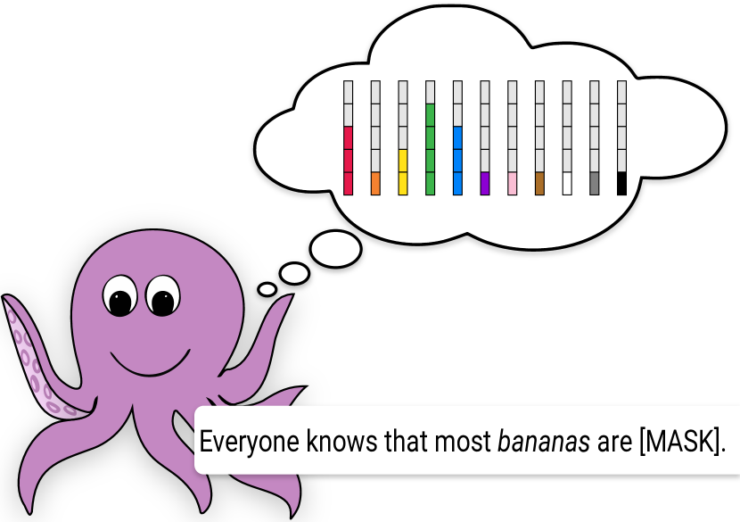
Figure 1: An example prompt from CoDa.

People’s understanding of color is primarily derived from their experience in the world. Every time we interact with an object, we update our understanding of the possible colors that object can take on. Further, we can often apply meaning to the differences: a green banana is unripe, a yellow banana is ideal, and a brown banana may be past its prime. Text-only LMs do not share this embodied experience. Similar to an octopus they cannot see colors, and need to rely solely on the inaccurate reporting of colors in text. Thus, we expect the colors LMs associate with objects to differ drastically from a human’s perception.

To test this hypothesis, we construct the Color Dataset (CoDa) – a ground-truth dataset of color distributions for 521 well-known objects via crowdsourcing. We use this dataset to compare the color distributions found in text and those predicted from LMs, finding that a LM’s shortcomings in recovering color distributions correlates with the reporting bias for those objects. Next, we hypothesize that models having access to multiple modalities, specifically vision and text, may be able to partially overcome these shortcoming by grounding the language to their limited visual experiences Bisk et al. (2020). To this end, we develop a unified framework for evaluating the color perception of text-only and multimodal architectures. Our results support the hypothesis that multimodal training can mitigate the effect of reporting bias.

Contributions We make three contributions: 1) We introduce a dataset with human color distributions for 521 well-known objects. 2) We conduct an extensive analysis to identify how reporting bias affects LMs’ perception of color. 3) We demonstrate that multimodal training mitigates, but not eliminates, the impact of reporting bias.

2 CoDa

2.1 Dataset Creation

Dataset	Count (Percentile)
	25%	50%	75%
Open Images V6	2.10K	3.96K	11.1K
Google Ngrams	1.63M	4.64M	25.4M
Wikipedia	2.04K	10.3K	38.8K
VQA	4	25	186

Table 1: Object frequencies in each domain/dataset after filtering. We report class label statistics for Open Images and $n$-gram frequencies for Google Ngrams, Wikipedia, and VQA prompts.

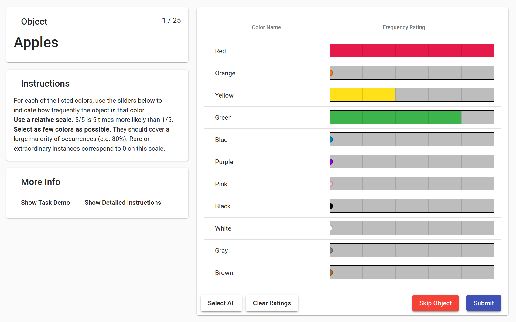
Figure 2: Our task UI for data collection on Amazon Mechanical Turk. See Section 2.1 for full details.

Object Selection

To ensure all our models – and potential future models – are properly exposed to the objects in our probing dataset, we choose objects which are common in both text and image data. We start with objects from the Open Images dataset Kuznetsova et al. (2020) and remove all objects which appear less than 25 times in Wikipedia. For example, we remove “dog bed” as the corresponding bi-gram only appears 19 times. This leaves us with an initial set of 687 objects.

We then manually filter out all human-related words, such as “person” as well as hypernyms such as “food”, since they are too general to assign specific colors. We also remove transparent objects, such as “windows”, and objects that are more than two words long, such as “personal flotation device” and “table tennis racket”. This leaves us with our final set of 521 objects. We provide object frequencies from Open Images V6 Kuznetsova et al. (2020), the Google Books Ngram Corpus Lin et al. (2012), Wikipedia, and VQA Goyal et al. (2017) in Table 1.

Color Selection

Following Berlin and Kay (1969), we choose the 11 basic color terms of the English language as the colors to be annotated: red, orange, yellow, green, blue, purple, pink, black, white, grey, and brown.

Color Annotation

Due to sample bias in image datasets Torralba and Efros (2011) and the difficulty of matching pixel values to human perception, generating color distributions by counting color frequencies in images is impractical and challenging to verify. Thus, in line with our focus on human perception of color as it relates to language (i.e., color terms), we approximate color distributions via human annotation crowdsourced on Amazon Mechanical Turk (MTurk).

Workers are shown words representing objects and tasked with rating – on a scale from 1 to 5 – the frequency with which instances of the objects appear in each of the 11 provided colors. We set up these tasks as human intelligence tasks (HITs), and provide the workers with instructions, which include an example for how one could label “grass” and a concrete list of acceptance and rejection criteria. Each HIT includes 25 objects and is compensated with $1. Fig. 2 shows the user interface as presented to an MTurk worker tasked with annotating the object “apples”.

Since we choose objects that appear frequently in datasets, we expect people to be familiar with them. However, for the rare cases where an annotator is unsure about an object’s color, our interface includes a skip button. The average crowdworker skips 1 object. If an object is not skipped, the average worker completes one annotation in 14 seconds on average. Each object’s annotation is normalized to obtain a probability distribution over colors.

A potential side-effect of crowdsourcing annotations is that annotators might choose fewer colors to minimize the time spent on the task. In light of this, we design a labeling interface that balances the time required for labeling a given object as one, many, or all colors. For example, we include a “Select All” button and use wide click-optimized sliders. With these changes, we find that, on average, users tend to select 6.2 colors per object. For more details and analysis regarding annotator biases, we refer the reader to Section A.1.

Quality Control

For quality control purposes, each HIT includes “spinach” as a control object at a random position within the group of objects to annotate. This control object serves as a way to flag any submissions which do not follow the instructions or are otherwise not suitable for our purposes. We require the rating of “spinach” to be more than 50% green in order to accept the HIT. Rejected HITs are not included in the dataset. This filters out the small number of workers who provide random or blatantly incorrect annotations.

We compute the ground truth as an average over all submitted annotations for a given object. We iteratively filter annotations on a per-object basis if a rating has a Kendall correlation of less than 0 with the current ground truth. This removes 10 annotations that appear to be cases of annotator misinterpretation. For example, one annotator labels “stop sign” as being equally red, yellow, and green, likely confusing “stop sign” with “traffic light”.

Group	All	Train	Val	Test	Examples
Single	198	118	39	41	Carrot, Spinach
Multi	208	124	41	43	Apple, Street light
Any	115	69	23	23	Shirt, Car
Total	521	311	103	107

Table 2: CoDa splits by object group.

Object Grouping

We are investigating the relationship between LMs’ knowledge of object colors and reporting bias, the tendency of humans to not state the obvious Grice (1975). We hypothesize that reporting bias will be more severe for objects which have a single typical color, as that color will be implicitly assumed by a listener or reader and, accordingly, will be less frequently stated explicitly. In contrast, objects with a distinct set of several possible colors require explicit descriptions to fully capture the visual characteristics of the object. For example, apples are often described as red or green.

To test whether objects with different color distributions are impacted by reporting bias differently, we divide the dataset into three categories: single-color objects, multi-color objects, and any-color objects. We categorize objects using $k$-means clustering with the Jensen-Shannon distance of sorted probabilities. This creates clusters which are color-invariant and based only on the properties of the distributions. We find that this method gives consistent clusters, i.e. the clusters are independent of seeding. We then assign group names semi-manually. “Lemon” is an example of a single color object, where 73% of the distribution is yellow. “Wine” is a multi-color object with 90% of the distribution falling on red, white, pink, and purple (the last 10% is yellow). All other objects are any-color objects: they have no clear set of typical colors. Examples of any-color objects are t-shirts, cars, or flowers. More examples are shown in Table 2.

Model Type	Input
Decoder	Most apples are $\mathbf{\left<O\right>}$.
Encoder	Most apples are $\mathbf{\left<M\right>}$.
CLIP	A photo of an apple.

Table 3: Example inputs for different evaluated architectures.

2.2 Templates

Text-only corpora and visually-grounded datasets rarely occupy the same domain. To accommodate both, we form a set of templates for each domain. The first is tailored to text-only models, and consists of both plural templates such as “Most bananas are [MASK].” and singular templates such as “This banana is [MASK]”.

Our second template group is tailored to visually-grounded datasets. We use most of the templates provided by Radford et al. (2021), which the authors used for finetuning on ImageNet, but exclude templates that inherently point to an unnatural object state, such as “a photo of a dirty banana”. Examples for templates are provided in Table 3.

We recognize that any hand-crafted templates are by nature imperfect. As such, we use all configurations for all models and present the best results per-object for each model to give models ample opportunity to succeed.

2.3 Data Splits

Some of our experiments (cf. Section 4.2) require a small training set. Thus, CoDa contains training, development and test splits, with 311, 103, and 106 objects respectively. There is no object overlap between the different sets.

Dataset	Group	Freq	Spearman $\rho\uparrow$	Kendall’s $\tau\uparrow$	Acc@1 $\uparrow$	$\mathbf{D_{JS}}\downarrow$
Google Ngrams	Single	$5.60$	$41.7\pm 27.8$	$35.3\pm 24.5$	43.9	$0.27\pm 0.16$
	Multi	$9.69$	$\textbf{47.1}\pm\textbf{26.6}$	$\textbf{38.1}\pm\textbf{22.2}$	$30.3$	$0.23\pm 0.12$
	Any	$20.26$	$43.5\pm 30.7$	$34.3\pm 25.0$	$33.9$	$\textbf{0.15}\pm\textbf{0.10}$
Wikipedia	Single	$1.51$	$26.5\pm 30.2$	$22.2\pm 26.3$	25.3	$0.37\pm 0.17$
	Multi	$1.85$	$29.4\pm 31.9$	$\textbf{23.9}\pm\textbf{27.0}$	$23.6$	$0.31\pm 0.16$
	Any	$3.00$	$\textbf{30.9}\pm\textbf{31.5}$	$23.8\pm 25.6$	$19.1$	$\textbf{0.23}\pm\textbf{0.15}$
VQA	Single	$0.73$	$27.4\pm 37.8$	$25.4\pm 35.3$	$16.7$	$0.38\pm 0.23$
	Multi	$2.17$	$\textbf{35.7}\pm\textbf{34.3}$	$\textbf{31.7}\pm\textbf{30.9}$	$21.2$	$0.35\pm 0.20$
	Any	$2.64$	$33.7\pm 33.6$	$28.1\pm 28.7$	27.8	$\textbf{0.29}\pm\textbf{0.17}$

Table 4: Correlation metrics between the $n$-gram frequencies reported in different datasets and the ground truth distributions collected from human annotators. Single, Multi, and Any indicate sets of objects that are frequently a single color, between two to four colors, or could be any color, respectively. We aggregate by object and report the mean $\pm$ standard deviation for each metric across the objects of that group.

3 Reporting Bias

3.1 Background

As previously stated, Grice’s conversational maxim of quantity manifests as reporting bias – i.e., people not usually stating obvious facts or properties –, and impacts nearly all datasets that contain text.

Reporting bias has been studied in the context of both NLP and image captioning. Gordon and Van Durme (2013) perform a quantitative analysis using n-gram frequencies from text, finding this phenomenon particularly relevant to internet text corpora. Shwartz and Choi (2020) extend these experiments to pretrained models such as Bert (Devlin et al., 2019) and RoBERTa (Liu et al., 2019). Similar to our work, they analyze color attribution of the form “The   banana is tasty.” However, their ground truth is extracted from Wikipedia bi-grams and, thus, suffers from reporting bias itself. In contrast, we circumvent this problem by collecting the ground truth in CoDa directly from humans.

3.2 Reporting Bias in Text

Our hypothesis is that pretrained LMs inherit reporting bias with respect to colors from their training data. Thus, prior to our main experiments, we investigate if, in fact, reporting bias exists in large general text corpora. We analyze the Google Books Ngram Corpus Lin et al. (2012) and Wikipedia. Specifically, we look at all bi-grams and tri-grams containing a color followed by an object in our dataset.

Let us denote the count of the $n$-gram $x_{1}\ldots x_{n}$ as $\phi(x_{1},\ldots,x_{n})$. We then define the relative frequency with which each object $o$ appears with a color $c$ as:

$$\textrm{Freq}(o)=\frac{100}{\phi(o)}\sum_{c\,\in\,C}\phi(c,o)$$ (1)

We further define the probability of an object being of color $c^{*}$ as:

$$P(c^{*}\,|\,o)=\frac{\phi(c^{*},o)}{\sum_{c\,\in\,C}\phi(c,o)}$$ (2)

The results of these experiments are reported in Table 4. The frequency column supports our hypothesis that objects with one typical color are less frequently described as being of any color than those with multiple typical colors or where any color is possible. In all metrics excluding Acc@1, the text-retrieved color distributions are more strongly correlated with the ground truth for multi and any colored objects than for single-colored objects.

4 Experimental Setup

Model	Sizes	Multimodal
GPT-2	B, M, L, XL
RoBERTa	B, L
ALBERT V1	B, L, XL, XXL
ALBERT V2	B, L, XL, XXL
CLIP	ViT-B/32, RN50,	✓
	RN50x4, RN101

Table 5: Summary of evaluated models.

4.1 Zero-shot Probes

We first probe LMs in a zero-shot fashion using a set of templates (see Section 2.2). Each template has a [MASK] where the color should appear. For models trained using a causal language modeling objective, we run the models over each template eleven times, each time with a different color replacing the [MASK] token. Following Warstadt et al. (2020), we select the sentence with the highest probability. For models trained using a masked language modeling objective, we filter the output vocabulary to only include the eleven color choices and normalize to obtain a probability distribution.

4.2 Representation Probes

Many current multimodal architectures are optimized for multimodal evaluation and have complex shared embedding spaces, which makes it challenging to compare to text-only models. However, recent developments such as CLIP Radford et al. (2021) and ALIGN Jia et al. (2021) show promising results in connecting images and text via contrastive pretraining on large unlabeled corpora, while still maintaining separate text and image models. We focus on probing multimodal models which follow these architecture decisions. Since they have not been trained on a language modeling objective, zero-shot probing is not viable on these models. To overcome this and enable comparison to text-only models, we freeze the base model and use part of our dataset to train a MLP to extract color distributions from the frozen representations.

Given pretrained representations, we would like the performance of a model to consist of 2 parts: final quality (in our case distribution correlations), and the amount of effort to get that quality from the representations. This is possible by formulating the task as efficiently learning a model from representations to color distributions. Following Whitney et al. (2021); Voita and Titov (2020), we conduct our experiments for representation probing in a loss-data framework using minimum description length (MDL), surplus description length (SDL), and $\varepsilon$ sample complexity ($\varepsilon SC$). We split the training set into 10 subsets spaced logarithmically from 1 to 311 objects, and report averages over 5 seeds.

Model	Group	Spearman $\rho\uparrow$	Kendall’s $\tau\uparrow$	Acc@1 $\uparrow$	$\mathbf{D_{JS}}\downarrow$	$\Delta\rho\uparrow$	$\Delta\tau\uparrow$
GPT-2	Single	$40.3\pm 26.6$	$33.6\pm 22.1$	40.4	$0.39\pm 0.07$	$-0.55$	$-1.01$
	Multi	$44.8\pm 20.9$	$36.5\pm 16.8$	$29.8$	$0.26\pm 0.06$	$-1.49$	$-1.05$
	Any	$\textbf{48.1}\pm\textbf{25.1}$	$\textbf{38.2}\pm\textbf{20.2}$	$40.0$	$\textbf{0.09}\pm\textbf{0.04}$	5.29	4.46
RoBERTa	Single	$47.8\pm 24.7$	$40.1\pm 20.8$	42.9	$0.28\pm 0.11$	$7.17$	$5.69$
	Multi	$50.2\pm 23.8$	$41.0\pm 19.5$	$33.2$	$0.19\pm 0.08$	$4.57$	$4.01$
	Any	$\textbf{52.5}\pm\textbf{23.5}$	$\textbf{42.0}\pm\textbf{19.5}$	$36.5$	$\textbf{0.10}\pm\textbf{0.06}$	9.97	8.26
ALBERT	Single	$43.7\pm 24.4$	$36.4\pm 20.6$	$34.3$	$0.30\pm 0.11$	$2.69$	$1.55$
	Multi	$44.6\pm 19.1$	$36.1\pm 15.5$	$26.9$	$0.22\pm 0.07$	$-1.53$	$-1.27$
	Any	$\textbf{48.2}\pm\textbf{21.4}$	$\textbf{38.2}\pm\textbf{17.2}$	35.7	$\textbf{0.11}\pm\textbf{0.05}$	5.07	4.22

Table 6: LM results when probed in a zero-shot setting. Single, Multi, and Any indicate sets of objects that are frequently of a single color, between two to four colors, or could be any color, respectively. All correlation coefficients ($\rho,\tau$) are multiplied by 100. For each object, we take the prediction from the template with the highest $\tau$ correlation. We then aggregate by object and report the mean $\pm$ standard deviation over objects of that group. We report the results from the best model from each architecture; for results on a per-model basis, see Table 9.

4.3 Models

We probe object-color probabilities in 14 pretrained text-only models as well as four versions of CLIP Radford et al. (2021). The text-only models are varied configurations of GPT-2 Radford et al. (2019), RoBERTa Liu et al. (2019), and ALBERT Lan et al. (2020); cf. Table 5 for the full set. We use Huggingface’s (Wolf et al., 2019) pretrained models for all text-only models and the official implementation of CLIP.

4.4 Metrics

In order to obtain as comprehensive a picture as possible, we report a variety of metrics when applicable, including: top-1 accuracy, Spearman rank order correlation $\rho$, Kendall rank correlation $\tau$, and Jensen-Shannon divergence $D_{JS}$ for each model and each set of objects. Each of these metrics highlight slightly different aspects of performance on the task.

Top-1 accuracy (Acc@1) is the frequency with which models can correctly identify the most frequent color of an object. This is useful for comparing models, but not directly interpretable across object groups as it inherently favors objects that can take on few colors. Spearman’s $\rho$ is sensitive to outliers, so it highlights the extreme mistakes, while Kendall’s $\tau$ is more robust to such changes. Jensen-Shannon divergence measures the similarity between 2 distributions.

Spearman’s $\rho$ and Kendall’s $\tau$ are within the range of $[-1,1]$, with -1 being negatively correlated and 1 being perfectly correlated. We additionally define $\Delta\rho$ and $\Delta\tau$ correlation difference measures defined on the interval [-100, 100], to compare model predictions to $n$-gram frequency predictions. This measures the difference in correlation between $n$-gram frequency predictions and a model’s probability distribution, where -100 indicates degraded correlation, 0 equals perfect correlation, and 100 indicates improved correlation with the ground truth as compared to the relative n-gram frequencies. In the context of reporting bias, $\Delta\rho$ and $\Delta\tau$ can be interpreted as measures of bias amplification or mitigation for negative and positive values, respectively.

We additionally define an average of the two correlation metrics as “Avg. Correlation”. When using this metric, we first compute $\frac{\rho+\tau}{2}$ for a specific object and perform all other aggregations in the same way as for the other metrics.

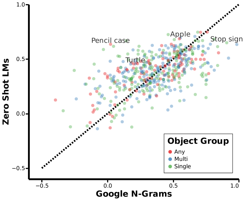
Figure 3: Correlation between n-gram frequency and LM performance for single, multi, and any color objects. X and Y axes are Kendall’s $\tau$ correlation between n-gram frequency and ground truth and LM predictions with ground truth respectively. Each point corresponds to a single object in our dataset. LM correlation is averaged over the top models for each architecture. The dotted line $y$=$x$ corresponds to to perfect correlation.

5 Results

5.1 Zero-Shot Probes

The results of LMs when probed in a zero-shot setting, provided in Table 6, clearly demonstrate that LMs perform worse on single-color objects and perform better on objects that can take on a range of colors. Furthermore, correlations are relatively low for all objects and models. This demonstrates that colors are generally challenging for state-of-the-art pretrained LMs.

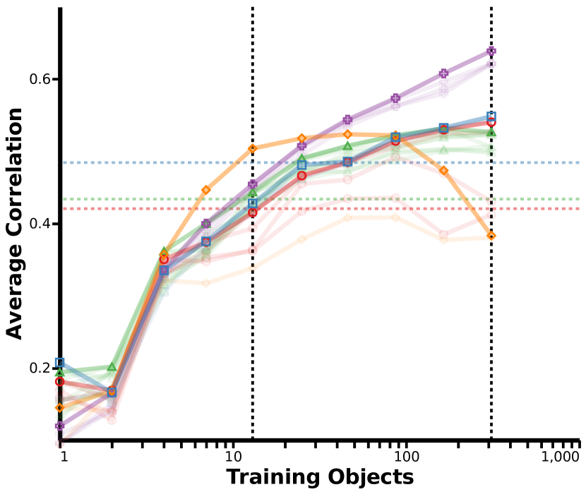
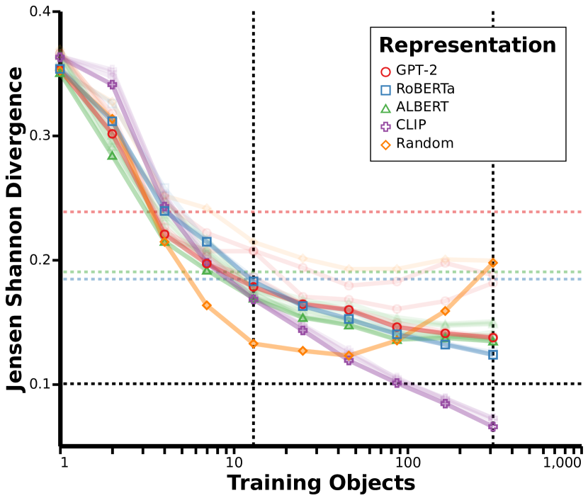
Figure 4: Representation probing results for unseen objects with varying amounts of data, averaged over 5 seeds. The main lines are the best model from those of the same type (e.g., RoBERTa_BASE and RoBERTa_LARGE), and the translucent lines are the per-model averages. Dotted lines represent best zero-shot performance for each model. The “Random” group consists of a randomly initialized RoBERTa and CLIP. The black dotted lines correspond to $\epsilon$ and $n$ in Table 8. Left: Average of Spearman’s $\rho$ and Kendall’s $\tau$. Right: Jensen-Shannon divergence.

5.2 Reporting Bias and Model Accuracy

Figure 3 compares the correlation between $n$-gram frequency and zero-shot LM performance. The identity line represents a theoretical perfect correlation between how well $n$-gram frequency correlates with our ground truth and LM predictions. Any points above the identity line represent cases where LMs seem to mitigate reporting bias – their predictions are closer to ground truth, and points below the line represent cases where LMs amplify reporting bias – their predictions are further from ground truth. When averaged across all models (see Appendix C for the full list of results) zero-shot LMs amplify the reporting bias of single-color objects by 5.23% on average, and 6.26% for multi-color objects. For any-color objects, we find a slight mitigation of 0.21% on average.

Table 7 aggregates and combines results from Tables 4 and 6 and elucidates two main points on the effect of reporting bias on a LM’s perception of color. First, the color distributions of LMs correlate more strongly with reporting bias-affected text than with a human’s perception of color. Second, single-colored objects are the most affected by reporting bias, and the objects LMs struggle the most on. These results indicate that, in line with our hypothesis, LMs are negatively impacted by reporting bias. Further, because reporting bias is innate to human communication and due to the enormous amount of text required for modern LMs, it is infeasible to eliminate reporting bias from all training data. This entails – in support of the arguments in Bender and Koller (2020) and Bisk et al. (2020) – that language understanding abilities are naturally limited by text-only training.

		Avg. Correlation $\uparrow$
Group	Freq.	Humans	Ngrams
Single	$5.60$	$40.1\pm 22.3$	$63.0\pm 18.1$
Multi	$9.69$	$42.2\pm 20.5$	$63.1\pm 17.5$
Any	$20.26$	$42.9\pm 22.5$	$\textbf{63.4}\pm\textbf{16.2}$

Table 7: LM predictions have higher correlation with n-gram frequencies. Here we compare the average correlation between LM predictions and two sources of “ground truth”; one collected from human annotators and one computed from n-gram frequencies. Single, Multi, and Any indicate sets of objects that are frequently of a single color, between two to four colors, or could be any color, respectively. The “Freq.” column indicates the frequency n-grams containing these objects also have one of the eleven colors.

		GPT-2	RoBERTa	CLIP
n		L	B	ViT-B/32
13	$\mathbf{D_{JS}}$	0.178	0.185	0.168
	MDL	2.80	2.95	2.79
	SDL, $\varepsilon$=0.1	> 1.50	> 1.65	> 1.49
	$\varepsilon$SC, $\varepsilon$=0.1	> 13	> 13	> 13
	Avg Corr.	40.7	42.7	45.5
311	$\mathbf{D_{JS}}$	0.137	0.123	0.065
	MDL	45.07	42.08	27.22
	SDL, $\varepsilon$=0.1	> 13.97	> 10.98	2.43
	$\varepsilon$SC, $\varepsilon$=0.1	> 311	> 311	165
	Avg Corr.	54.0	54.9	63.9

Table 8: Estimated measures of representation quality for the best model of each architecture.

5.3 Representation Probes

Fig. 4 shows the average correlation and Jensen-Shannon divergence for unseen objects as a function of the number of training objects. Note that with 14 objects, all models surpass zero-shot performance in terms of Jensen-Shannon divergence. With enough training objects, we observe similar ranking patterns observed in the zero-shot setting for text-only models. However, the advantage of this approach is that we can additionally include multimodal architectures.

The results from these experiments demonstrate that multimodal models outperform text-only models at recovering color distributions. They manage to do so even though the performance of multimodal models is often lower on classic NLP tasks Tan and Bansal (2020) and many multimodal datasets are even more prone to reporting bias in text Misra et al. (2016); van Miltenburg (2016); Burns et al. (2018). This further support the arguments in Bisk et al. (2020) that understanding concepts requires experiencing them in their natural form.

6 Limitations

While our work identifies issues with text-only training and motivates the use of multimodal signals during pretraining, in this section we outline some limitations of our approach.

First, a number of recent papers have highlighted potential limitations of probing LMs in certain ways Zhang and Bowman (2018); Whitney et al. (2021). While we acknowledge that probing does not provide a full picture of the capabilities of LMs, our hypothesis was supported by a range of different results from different approaches. In future work, we hope to leverage research (Bouraoui et al., 2020; Jiang et al., 2020) that demonstrates effective methods for automatically producing templates optimized for specific models. In the current state, we cannot and do not state exactly what LMs do and do not capture, rather we use our results to uphold and strengthen our original hypothesis that reporting bias hinders performance and that multimodal signals can help mitigate this problem.

Second, the bi-gram/tri-gram approach we use to quantify reporting bias only approximates the full set of object-color instances. To be more exact, a dependency parser would have to be run on every dataset.

Finally, although our results motivate the use of multimodal signals during pretraining, there are still challenges to overcome. As discussed by Tan and Bansal (2020), the performance of multimodal models on classic NLP tasks often does not reflect the inherent advantages of these architectures, and many multimodal dataset are even more prone to reporting bias in text Misra et al. (2016); van Miltenburg (2016); Burns et al. (2018). Further, while a visual signal is able to better impart a sense of color, it is not enough to endow models with the meaning behind those colors. Humans easily learn that a green banana is not yet ripe, and that a brown banana is past its prime. For models to obtain this level of knowledge and reasoning they will likely require training signals from more modalities, and potentially fully embodied experiences.

7 Related Work

Color-Object Relationships Preexisting word association datasets often include object-color relationships as either having multiple equally likely pairings Gladkova et al. (2016); Kucera and Francis (1967), or as probabilistic cue-target pairs (Nelson et al., 2004). Others such as Devereux et al. (2013) take a norm completion approach, wherein participants are tasked with generating attributes given some concept. One can then extract the object-color relationships by counting the number of participants who reported a given color.

However, the resulting “distribution” is an aggregate count over individuals, and does not necessarily reflect the distribution from the eyes of a single observer. Thus, previous research into LMs as knowledge bases has not been able to fully explore the extent to which they know color A. Rodriguez and Merlo (2020); Shwartz and Choi (2020).

Previous work has shown the importance of color in visual perception and object recognition Rosenthal et al. (2018); Gegenfurtner and Rieger (2000). More recently Teichmann et al. (2020) use time resolved neural imaging data to demonstrate how the typicality of object-color relationships influences object representations in visual processing.

Probing LMs

A wide range of papers have probed LMs in a zero-shot fashion by looking at how they fill in a [MASK] token in handcrafted Weir et al. (2020); Petroni et al. (2019); Jiang et al. (2020); Ettinger (2020); Lin et al. (2020) or automatically generated Bouraoui et al. (2020); Jiang et al. (2020) template sentences. Others, such as Warstadt et al. (2020) compare perplexities between minimal pairs of sentences. A different approach is to analyze the representation quality of LMs for linguistic tasks by training a simple MLP on pretrained model representations (Da and Kasai, 2019; Lin et al., 2019). However, Zhang and Bowman (2018) demonstrate that the procedure of training an additional classifier may distort the results. An alternative approach introduced by Voita and Titov (2020) is information-theoretic probing with MDL. This method builds on standard probing classifiers by not only measuring the final performance, but additionally measuring the amount of effort required to achieve that performance.

Probing Multimodal LMs

Often multimodal LMs are used in the domain of visual question answering, where, given an image, the model is asked a question about concepts in the image Goyal et al. (2017); Hudson and Manning (2019). While it is often possible to simply use the text-only portion of these models for other tasks, this often leads to poor performance on solely language-based tasks (Tan and Bansal, 2020).

8 Conclusion

In this paper we investigate how reporting bias negatively effects a LM’s perception of color. We do so by first creating CoDa, a dataset of 521 human-perceived color distributions for common objects. We then utilize this dataset to demonstrate that text-only models are inherently limited because of reporting bias. Subsequently, we show that multimodal training mitigates these issues. Overall, our results support the claims in Bender and Koller (2020) and Bisk et al. (2020) that text-only training is insufficient for language understanding and motivate further research on how to best employ multimodal training signals.

Appendix A Dataset Construction

A.1 Analysis of Annotator Biases

A potential side-effect of crowdsourcing annotations is that annotators might be biased toward choosing fewer colors faster, as this would equate to higher monetary incentives. We observe a small correlation (Kendall’s Tau=0.154, p=0.026) between the total time and number of colors selected. However, this is to be expected as selecting the colors takes time.

All models we evaluate were predominately trained on English text. To accommodate this domain and minimize dataset variance, we recruit only annotators from the United States. This may induce cultural or geographic biases: e.g., the color diversity of carrots is much smaller in the United States than in some Asian countries. Other geographic biases are more fine-grained; for example, the color of fire hydrants in the U.S. depends on where you live and the water source.

Additionally, our choice of colors is not as universal as, for example, the 6 color terms defined by The World Color Survey Kay et al. (2009). The latter may be more suitable for multilingual studies, though we leave such investigations for future work.

Appendix B Experimental Details

For all experiments, we implement the CoDa dataset using the Huggingface Datasets Library. We use Huggingface’s (Wolf et al., 2019) pretrained models for evaluating all text-only models, and the official CLIP implementation by Radford et al. (2021) for all CLIP models. We run all experiments on a single machine with one Nvidia Titan RTX GPU.

B.1 Representation Probing

Our representation probing implementation is derived from the efficient JAX version provided by Whitney et al. (2021).

We split the training set into 10 subsets spaced logarithmically from 1 to 311 objects, and report averages over 5 seeds. Note that for each seed, any additional points along the curve represent additional objects to the previous subset, however, different seeds have different object sets and thus a different number of samples per subset. For our dataset, we found the difference in samples to be far less impactful on performance than the number of objects.

All probes are 2-layer MLPs with ReLU activation functions and are trained using the Adam Optimizer Kingma and Ba (2015) with a learning rate of $10^{-4}$. All probes are trained for 4000 steps. More details on how to reproduce the experiments are provided in our GitHub repository.

Appendix C Zero Shot Results

The zero-shot results for all evaluated LMs are provided in Table 9.

Model		Group	Spearman $\rho\uparrow$	Kendall’s $\tau\uparrow$	Acc@1 $\uparrow$	$\mathbf{D_{JS}}\downarrow$	$\Delta\rho\uparrow$	$\Delta\tau\uparrow$
GPT-2	B	Single	$34.9\pm 25.7$	$28.8\pm 21.2$	$26.8$	$0.39\pm 0.07$	$-6.86$	$-6.60$
		Multi	$40.7\pm 22.9$	$32.9\pm 18.5$	$23.6$	$0.25\pm 0.06$	$-6.77$	$-5.46$
		Any	$\textbf{45.7}\pm\textbf{25.0}$	$\textbf{36.9}\pm\textbf{20.9}$	33.9	$\textbf{0.09}\pm\textbf{0.04}$	2.17	2.64
	M	Single	$34.2\pm 26.4$	$28.5\pm 21.8$	35.9	$0.39\pm 0.07$	$-6.94$	$-6.30$
		Multi	$36.0\pm 26.0$	$29.5\pm 20.8$	$25.5$	$0.25\pm 0.06$	$-10.87$	$-8.51$
		Any	$\textbf{43.2}\pm\textbf{26.5}$	$\textbf{34.8}\pm\textbf{21.2}$	$35.7$	$\textbf{0.09}\pm\textbf{0.04}$	0.09	0.74
	L	Single	$39.9\pm 24.4$	$32.8\pm 19.7$	$33.8$	$0.39\pm 0.07$	$-1.10$	$-1.91$
		Multi	$44.8\pm 20.9$	$36.5\pm 16.8$	$29.8$	$0.26\pm 0.06$	$-1.49$	$-1.05$
		Any	$\textbf{47.3}\pm\textbf{26.9}$	$\textbf{37.9}\pm\textbf{21.8}$	38.3	$\textbf{0.09}\pm\textbf{0.04}$	4.35	3.95
	XL	Single	$40.3\pm 26.6$	$33.6\pm 22.1$	40.4	$0.39\pm 0.07$	$-0.55$	$-1.01$
		Multi	$41.7\pm 24.3$	$34.1\pm 19.4$	$28.8$	$0.25\pm 0.06$	$-4.66$	$-3.42$
		Any	$\textbf{48.1}\pm\textbf{25.1}$	$\textbf{38.2}\pm\textbf{20.2}$	$40.0$	$\textbf{0.09}\pm\textbf{0.04}$	5.29	4.46
RoBERTa	B	Single	$41.5\pm 23.9$	$34.4\pm 19.6$	32.3	$0.32\pm 0.13$	$0.58$	$-0.21$
		Multi	$47.0\pm 21.9$	$37.7\pm 18.0$	$23.1$	$0.21\pm 0.09$	$0.44$	$-0.03$
		Any	$\textbf{51.9}\pm\textbf{22.7}$	$\textbf{41.3}\pm\textbf{18.9}$	$29.6$	$\textbf{0.11}\pm\textbf{0.07}$	8.64	7.27
	L	Single	$47.8\pm 24.7$	$40.1\pm 20.8$	42.9	$0.28\pm 0.11$	$7.17$	$5.69$
		Multi	$50.2\pm 23.8$	$41.0\pm 19.5$	$33.2$	$0.19\pm 0.08$	$4.57$	$4.01$
		Any	$\textbf{52.5}\pm\textbf{23.5}$	$\textbf{42.0}\pm\textbf{19.5}$	$36.5$	$\textbf{0.10}\pm\textbf{0.06}$	9.97	8.26
ALBERT V1	B	Single	$27.8\pm 25.0$	$23.2\pm 20.3$	$16.2$	$0.38\pm 0.10$	$-14.08$	$-12.30$
		Multi	$31.4\pm 24.2$	$25.1\pm 18.8$	$13.0$	$0.27\pm 0.09$	$-15.27$	$-12.60$
		Any	$\textbf{42.8}\pm\textbf{26.4}$	$\textbf{33.7}\pm\textbf{21.4}$	18.3	$\textbf{0.14}\pm\textbf{0.06}$	-0.70	-0.63
	L	Single	$29.4\pm 27.0$	$24.3\pm 21.9$	$31.8$	$0.35\pm 0.13$	$-11.67$	$-10.62$
		Multi	$32.7\pm 22.6$	$26.7\pm 18.0$	$23.1$	$0.25\pm 0.09$	$-13.50$	$-10.78$
		Any	$\textbf{41.2}\pm\textbf{25.7}$	$\textbf{33.6}\pm\textbf{20.5}$	38.3	$\textbf{0.13}\pm\textbf{0.06}$	-2.37	-0.58
	XL	Single	$36.4\pm 24.5$	$29.7\pm 20.0$	$26.3$	$0.35\pm 0.11$	$-4.73$	$-4.99$
		Multi	$44.6\pm 19.1$	$36.1\pm 15.5$	$26.9$	$0.22\pm 0.07$	$-1.53$	$-1.27$
		Any	$\textbf{48.2}\pm\textbf{21.4}$	$\textbf{38.2}\pm\textbf{17.2}$	35.7	$\textbf{0.11}\pm\textbf{0.05}$	5.07	4.22
	XXL	Single	$39.9\pm 25.6$	$33.1\pm 21.1$	$31.3$	$0.31\pm 0.12$	$-1.38$	$-1.80$
		Multi	$41.3\pm 26.1$	$\textbf{33.2}\pm\textbf{21.0}$	$23.6$	$0.21\pm 0.08$	$-5.23$	$-4.48$
		Any	$\textbf{41.9}\pm\textbf{24.3}$	$32.8\pm 18.4$	38.3	$\textbf{0.11}\pm\textbf{0.05}$	-0.87	-1.03
ALBERT V2	B	Single	$22.3\pm 29.7$	$18.9\pm 24.2$	$20.7$	$0.36\pm 0.11$	$-19.54$	$-16.46$
		Multi	$22.2\pm 26.8$	$18.0\pm 21.3$	$18.3$	$0.26\pm 0.07$	$-23.57$	$-19.11$
		Any	$\textbf{25.8}\pm\textbf{26.9}$	$\textbf{20.8}\pm\textbf{20.6}$	26.1	$\textbf{0.12}\pm\textbf{0.05}$	-18.38	-13.98
	L	Single	$39.2\pm 27.1$	$32.5\pm 22.4$	$30.3$	$0.32\pm 0.11$	-2.14	$-2.50$
		Multi	$\textbf{41.9}\pm\textbf{24.9}$	$\textbf{33.9}\pm\textbf{20.4}$	$25.0$	$0.21\pm 0.07$	$-3.73$	$-3.10$
		Any	$40.0\pm 22.9$	$32.4\pm 18.1$	33.0	$\textbf{0.10}\pm\textbf{0.05}$	$-3.70$	-2.05
	XL	Single	$25.2\pm 26.6$	$20.5\pm 21.5$	26.3	$0.35\pm 0.12$	$-16.14$	$-14.53$
		Multi	$25.4\pm 23.4$	$20.7\pm 18.4$	$23.6$	$0.25\pm 0.08$	$-20.51$	$-16.59$
		Any	$\textbf{29.6}\pm\textbf{27.1}$	$\textbf{23.1}\pm\textbf{20.8}$	$26.1$	$\textbf{0.12}\pm\textbf{0.05}$	-12.48	-10.04
	XXL	Single	$43.7\pm 24.4$	$\textbf{36.4}\pm\textbf{20.6}$	$34.3$	$0.30\pm 0.11$	2.69	1.55
		Multi	$\textbf{45.2}\pm\textbf{23.7}$	$36.1\pm 19.5$	$25.5$	$0.20\pm 0.07$	$-1.08$	$-1.40$
		Any	$43.7\pm 24.9$	$34.5\pm 19.6$	39.1	$\textbf{0.10}\pm\textbf{0.05}$	$0.95$	$0.70$
Average		Single	$35.9\pm 25.8$	$29.8\pm 21.2$	$30.7$	$0.35\pm 0.10$	$-5.33$	$-5.14$
		Multi	$38.9\pm 23.6$	$31.5\pm 19.0$	$24.5$	$0.24\pm 0.07$	$-7.37$	$-5.99$
		Any	$\textbf{43.0}\pm\textbf{25.0}$	$\textbf{34.3}\pm\textbf{19.9}$	33.5	$\textbf{0.11}\pm\textbf{0.05}$	-0.14	0.28

Table 9: LM results when probed in a zero-shot setting. Single, Multi, and Any indicate sets of objects that are frequently a singe color, between two to four colors, or could be any color, respectively. All correlation coefficients ($\rho,\tau$) are multiplied by 100. Means and standard deviations are calculated over objects of the respective group.

References

- A. Rodriguez and Merlo (2020) Maria A. Rodriguez and Paola Merlo. 2020. Word associations and the distance properties of context-aware word embeddings. In Proceedings of the 24th Conference on Computational Natural Language Learning, pages 376–385, Online. Association for Computational Linguistics.
- Aroca-Ouellette et al. (2021) Stéphane Aroca-Ouellette, Cory Paik, Alessandro Roncone, and Katharina Kann. 2021. PROST: Physical reasoning about objects through space and time. In Findings of the Association for Computational Linguistics: ACL-IJCNLP 2021, pages 4597–4608, Online. Association for Computational Linguistics.
- Bender and Koller (2020) Emily M. Bender and Alexander Koller. 2020. Climbing towards NLU: On meaning, form, and understanding in the age of data. In Proceedings of the 58th Annual Meeting of the Association for Computational Linguistics, pages 5185–5198, Online. Association for Computational Linguistics.
- Berlin and Kay (1969) Brent Berlin and Paul Kay. 1969. Basic Color Terms: Their Universality and Evolution. University of California Press.
- Bisk et al. (2020) Yonatan Bisk, Ari Holtzman, Jesse Thomason, Jacob Andreas, Yoshua Bengio, Joyce Chai, Mirella Lapata, Angeliki Lazaridou, Jonathan May, Aleksandr Nisnevich, Nicolas Pinto, and Joseph Turian. 2020. Experience grounds language. In Proceedings of the 2020 Conference on Empirical Methods in Natural Language Processing (EMNLP), pages 8718–8735, Online. Association for Computational Linguistics.
- Bouraoui et al. (2020) Zied Bouraoui, José Camacho-Collados, and Steven Schockaert. 2020. Inducing relational knowledge from BERT. In The Thirty-Fourth AAAI Conference on Artificial Intelligence, AAAI 2020, The Thirty-Second Innovative Applications of Artificial Intelligence Conference, IAAI 2020, The Tenth AAAI Symposium on Educational Advances in Artificial Intelligence, EAAI 2020, New York, NY, USA, February 7-12, 2020, pages 7456–7463. AAAI Press.
- Burns et al. (2018) Kaylee Burns, Lisa Anne Hendricks, Trevor Darrell, and Anna Rohrbach. 2018. Women also snowboard: Overcoming bias in captioning models. ArXiv preprint, abs/1803.09797.
- Da and Kasai (2019) Jeff Da and Jungo Kasai. 2019. Cracking the contextual commonsense code: Understanding commonsense reasoning aptitude of deep contextual representations. In Proceedings of the First Workshop on Commonsense Inference in Natural Language Processing, pages 1–12, Hong Kong, China. Association for Computational Linguistics.
- Devereux et al. (2013) Barry Devereux, Lorraine Tyler, Jeroen Geertzen, and Billi Randall. 2013. The centre for speech, language and the brain (cslb) concept property norms. Behavior research methods, 46.
- Devlin et al. (2019) Jacob Devlin, Ming-Wei Chang, Kenton Lee, and Kristina Toutanova. 2019. BERT: Pre-training of deep bidirectional transformers for language understanding. In Proceedings of the 2019 Conference of the North American Chapter of the Association for Computational Linguistics: Human Language Technologies, Volume 1 (Long and Short Papers), pages 4171–4186, Minneapolis, Minnesota. Association for Computational Linguistics.
- Ettinger (2020) Allyson Ettinger. 2020. What BERT is not: Lessons from a new suite of psycholinguistic diagnostics for language models. Transactions of the Association for Computational Linguistics, 8:34–48.
- Gegenfurtner and Rieger (2000) Karl R Gegenfurtner and Jochem Rieger. 2000. Sensory and cognitive contributions of color to the recognition of natural scenes. Current Biology, 10(13):805–808.
- Gladkova et al. (2016) Anna Gladkova, Aleksandr Drozd, and Satoshi Matsuoka. 2016. Analogy-based detection of morphological and semantic relations with word embeddings: what works and what doesn’t. In Proceedings of the NAACL Student Research Workshop, pages 8–15, San Diego, California. Association for Computational Linguistics.
- Gordon and Van Durme (2013) Jonathan Gordon and Benjamin Van Durme. 2013. Reporting bias and knowledge acquisition. In Proceedings of the 2013 workshop on Automated knowledge base construction, pages 25–30.
- Goyal et al. (2017) Yash Goyal, Tejas Khot, Douglas Summers-Stay, Dhruv Batra, and Devi Parikh. 2017. Making the V in VQA matter: Elevating the role of image understanding in visual question answering. In 2017 IEEE Conference on Computer Vision and Pattern Recognition, CVPR 2017, Honolulu, HI, USA, July 21-26, 2017, pages 6325–6334. IEEE Computer Society.
- Grice (1975) Herbert P Grice. 1975. Logic and conversation. In Speech acts, pages 41–58. Brill.
- Hudson and Manning (2019) Drew A. Hudson and Christopher D. Manning. 2019. GQA: A new dataset for real-world visual reasoning and compositional question answering. In IEEE Conference on Computer Vision and Pattern Recognition, CVPR 2019, Long Beach, CA, USA, June 16-20, 2019, pages 6700–6709. Computer Vision Foundation / IEEE.
- Jia et al. (2021) Chao Jia, Yinfei Yang, Ye Xia, Yi-Ting Chen, Zarana Parekh, Hieu Pham, Quoc V. Le, Yunhsuan Sung, Zhen Li, and Tom Duerig. 2021. Scaling up visual and vision-language representation learning with noisy text supervision.
- Jiang et al. (2020) Zhengbao Jiang, Frank F. Xu, Jun Araki, and Graham Neubig. 2020. How can we know what language models know? Transactions of the Association for Computational Linguistics, 8:423–438.
- Kay et al. (2009) Paul Kay, Brent Berlin, Luisa Maffi, William R Merrifield, and Richard Cook. 2009. The world color survey. CSLI Publications Stanford, CA.
- Kingma and Ba (2015) Diederik P. Kingma and Jimmy Ba. 2015. Adam: A method for stochastic optimization. In 3rd International Conference on Learning Representations, ICLR 2015, San Diego, CA, USA, May 7-9, 2015, Conference Track Proceedings.
- Kucera and Francis (1967) H. Kucera and W. N. Francis. 1967. Computational analysis of present-day American English. Brown University Press, Providence, RI.
- Kuznetsova et al. (2020) Alina Kuznetsova, Hassan Rom, Neil Alldrin, Jasper Uijlings, Ivan Krasin, Jordi Pont-Tuset, Shahab Kamali, Stefan Popov, Matteo Malloci, Alexander Kolesnikov, and et al. 2020. The open images dataset v4. International Journal of Computer Vision, 128(7):1956–1981.
- Lan et al. (2020) Zhenzhong Lan, Mingda Chen, Sebastian Goodman, Kevin Gimpel, Piyush Sharma, and Radu Soricut. 2020. ALBERT: A lite BERT for self-supervised learning of language representations. In 8th International Conference on Learning Representations, ICLR 2020, Addis Ababa, Ethiopia, April 26-30, 2020. OpenReview.net.
- Lin et al. (2020) Bill Yuchen Lin, Seyeon Lee, Rahul Khanna, and Xiang Ren. 2020. Birds have four legs?! NumerSense: Probing Numerical Commonsense Knowledge of Pre-Trained Language Models. In Proceedings of the 2020 Conference on Empirical Methods in Natural Language Processing (EMNLP), pages 6862–6868, Online. Association for Computational Linguistics.
- Lin et al. (2019) Yongjie Lin, Yi Chern Tan, and Robert Frank. 2019. Open sesame: Getting inside BERT’s linguistic knowledge. In Proceedings of the 2019 ACL Workshop BlackboxNLP: Analyzing and Interpreting Neural Networks for NLP, pages 241–253, Florence, Italy. Association for Computational Linguistics.
- Lin et al. (2012) Yuri Lin, Jean-Baptiste Michel, Erez Aiden Lieberman, Jon Orwant, Will Brockman, and Slav Petrov. 2012. Syntactic annotations for the Google Books NGram corpus. In Proceedings of the ACL 2012 System Demonstrations, pages 169–174, Jeju Island, Korea. Association for Computational Linguistics.
- Liu et al. (2019) Yinhan Liu, Myle Ott, Naman Goyal, Jingfei Du, Mandar Joshi, Danqi Chen, Omer Levy, Mike Lewis, Luke Zettlemoyer, and Veselin Stoyanov. 2019. Roberta: A robustly optimized bert pretraining approach. ArXiv preprint, abs/1907.11692.
- Misra et al. (2016) Ishan Misra, C. Lawrence Zitnick, Margaret Mitchell, and Ross B. Girshick. 2016. Seeing through the human reporting bias: Visual classifiers from noisy human-centric labels. In 2016 IEEE Conference on Computer Vision and Pattern Recognition, CVPR 2016, Las Vegas, NV, USA, June 27-30, 2016, pages 2930–2939. IEEE Computer Society.
- Nelson et al. (2004) Douglas L Nelson, Cathy L McEvoy, and Thomas A Schreiber. 2004. The university of south florida free association, rhyme, and word fragment norms. Behavior Research Methods, Instruments, & Computers, 36(3):402–407.
- Petroni et al. (2019) Fabio Petroni, Tim Rocktäschel, Sebastian Riedel, Patrick Lewis, Anton Bakhtin, Yuxiang Wu, and Alexander Miller. 2019. Language models as knowledge bases? In Proceedings of the 2019 Conference on Empirical Methods in Natural Language Processing and the 9th International Joint Conference on Natural Language Processing (EMNLP-IJCNLP), pages 2463–2473, Hong Kong, China. Association for Computational Linguistics.
- Radford et al. (2021) Alec Radford, Jong Wook Kim, Chris Hallacy, Aditya Ramesh, Gabriel Goh, Sandhini Agarwal, Girish Sastry, Amanda Askell, Pamela Mishkin, Jack Clark, Gretchen Krueger, and Ilya Sutskever. 2021. Learning transferable visual models from natural language supervision.
- Radford et al. (2019) Alec Radford, Jeffrey Wu, Rewon Child, David Luan, Dario Amodei, and Ilya Sutskever. 2019. Language models are unsupervised multitask learners. OpenAI blog, 1(8):9.
- Rosenthal et al. (2018) Isabelle Rosenthal, Sivalogeswaran Ratnasingam, Theodros Haile, Serena Eastman, Josh Fuller-Deets, and Bevil R. Conway. 2018. Color statistics of objects, and color tuning of object cortex in macaque monkey. Journal of Vision, 18(11):1–1.
- Shwartz and Choi (2020) Vered Shwartz and Yejin Choi. 2020. Do neural language models overcome reporting bias? In Proceedings of the 28th International Conference on Computational Linguistics, pages 6863–6870, Barcelona, Spain (Online). International Committee on Computational Linguistics.
- Tan and Bansal (2020) Hao Tan and Mohit Bansal. 2020. Vokenization: Improving language understanding with contextualized, visual-grounded supervision. In Proceedings of the 2020 Conference on Empirical Methods in Natural Language Processing (EMNLP), pages 2066–2080, Online. Association for Computational Linguistics.
- Teichmann et al. (2020) Lina Teichmann, Genevieve L. Quek, Amanda K. Robinson, Tijl Grootswagers, Thomas A. Carlson, and Anina N. Rich. 2020. The influence of object-color knowledge on emerging object representations in the brain. Journal of Neuroscience, 40(35):6779–6789.
- Torralba and Efros (2011) Antonio Torralba and Alexei A. Efros. 2011. Unbiased look at dataset bias. In The 24th IEEE Conference on Computer Vision and Pattern Recognition, CVPR 2011, Colorado Springs, CO, USA, 20-25 June 2011, pages 1521–1528. IEEE Computer Society.
- van Miltenburg (2016) Emiel van Miltenburg. 2016. Stereotyping and bias in the flickr30k dataset. ArXiv preprint, abs/1605.06083.
- Voita and Titov (2020) Elena Voita and Ivan Titov. 2020. Information-theoretic probing with minimum description length. In Proceedings of the 2020 Conference on Empirical Methods in Natural Language Processing (EMNLP), pages 183–196, Online. Association for Computational Linguistics.
- Warstadt et al. (2020) Alex Warstadt, Alicia Parrish, Haokun Liu, Anhad Mohananey, Wei Peng, Sheng-Fu Wang, and Samuel R. Bowman. 2020. BLiMP: The benchmark of linguistic minimal pairs for English. Transactions of the Association for Computational Linguistics, 8:377–392.
- Weir et al. (2020) Nathaniel Weir, Adam Poliak, and Benjamin Van Durme. 2020. Probing neural language models for human tacit assumptions. CogSci.
- Whitney et al. (2021) William F. Whitney, Min Jae Song, David Brandfonbrener, Jaan Altosaar, and Kyunghyun Cho. 2021. Evaluating representations by the complexity of learning low-loss predictors.
- Wolf et al. (2019) Thomas Wolf, Lysandre Debut, Victor Sanh, Julien Chaumond, Clement Delangue, Anthony Moi, Pierric Cistac, Tim Rault, Rémi Louf, Morgan Funtowicz, Joe Davison, Sam Shleifer, Patrick von Platen, Clara Ma, Yacine Jernite, Julien Plu, Canwen Xu, Teven Le Scao, Sylvain Gugger, Mariama Drame, Quentin Lhoest, and Alexander M. Rush. 2019. Huggingface’s transformers: State-of-the-art natural language processing. ArXiv preprint, abs/1910.03771.
- Zhang and Bowman (2018) Kelly Zhang and Samuel Bowman. 2018. Language modeling teaches you more than translation does: Lessons learned through auxiliary syntactic task analysis. In Proceedings of the 2018 EMNLP Workshop BlackboxNLP: Analyzing and Interpreting Neural Networks for NLP, pages 359–361, Brussels, Belgium. Association for Computational Linguistics.