Simulation of emergence in artificial societies:
a practical model-based approach
with the EB-DEVS formalism

Abstract

Modelling and simulation of complex systems is key to exploring and understanding social processes, benefiting from formal mechanisms to derive global-level properties from local-level interactions. In this paper we extend the body of knowledge on formal methods in complex systems by applying EB-DEVS, a novel formalism tailored for the modelling, simulation and live identification of emergent properties. We guide the reader through the implementation of different classical models for varied social systems to introduce good modelling practices and showcase the advantages and limitations of modelling emergence with EB-DEVS, in particular through its live emergence detection capability. This work provides case study-driven evidence for the neatness and compactness of the approach to modelling communication structures that can be explicit or implicit, static or dynamic, with or without multilevel interactions, and with weak or strong emergent behaviour. Throughout examples we show that EB-DEVS permits conceptualising the analysed societies by incorporating emergent behaviour when required, namely by integrating as a macro-level aggregate the Gini index in the Sugarscape model, Fads and Fashion in the Dissemination of Culture model, size-biased degree distribution in a Preferential Attachment model, happiness index in the Segregation model and quarantines in the SIR epidemic model. We also show in practice that the formalism and its implementation are backward compatible with Classic DEVS, allowing the incremental extension of previously developed models with new features provided by EB-DEVS. In each example we discuss the role of communication structures in the development of multilevel simulation models, and illustrate how micro-macro feedback loops enable the modelling of macro-level properties. Our results stress the relevance of multilevel features to support a robust approach in the modelling and simulation of complex systems.

Keywords Complex Systems Simulation  $\cdot$ DEVS  $\cdot$ Emergent Behaviour  $\cdot$ Agent Based Models

1 Introduction

Agent Based Modelling (ABM) has proven a very successful simulation-driven tool to explain phenomena, discover new questions and challenge prevailing theories. In Why model? (Epstein, 2008) the author proposes a comprehensive guide in a broad spectrum of good reasons to model. The social sciences have found computer simulation to be a valuable technique for experimenting with social models and hypothetical scenarios. Noteworthy models in the literature cover multiple disciplines such as political science (Axelrod, 1997; Schelling, 1971), economics (Tesfatsion, 2002), sociology (Macy and Willer, 2002) and epidemiology (Kermack and McKendrick, 1927), just to name a few.

According to Edmonds and Hales (2005) “[models] play a supporting role to the main argument. In many cases, if a paper that uses such a model were rewritten without it, the conclusions would not greatly differ, but rather the formal model is a concrete expression and demonstration of the processes being discussed” .

Research in artificial societies benefits from formal modelling as it supports new theories in a concise, correct and unambiguous fashion. According to Sawyer (2005) complex systems’ theory is key to understand complex dynamical systems such as societies and emergence is a key element that allows for multiple levels of analysis. Consequently, integrating higher and lower levels of abstraction with powerful tools may help the modeller to gain deeper understanding of the system under study.

In this paper we extend the body of knowledge on formal methods in complex systems by applying a novel formalism tailored for the modelling, simulation and live identification of emergent properties.

Emergent patterns, structures and properties need to be conceptualised. Authors from the social sciences have acknowledged that top-down approaches are inefficient due to the extensive knowledge needed for its formalisation, while bottom-up modelling provides better means to understand social systems. Agent based modelling, helps to understand global properties as emergent properties of actors interactions. In Macy’s words: “we may be able to understand these dynamics much better by trying to model them, not at the global level but instead as emergent properties of local interaction among adaptive agents who influence one another in response to the influence they receive.” Macy and Willer (2002, p. 144)

In this work we introduce good modelling practices for complex systems with EB-DEVS (Foguelman et al., 2021), a formalism designed to deal explicitly with emergent properties. We guide the reader through the implementation of classical models in social sciences based on this formalism. Our goal is to showcase the advantages and limitations of modelling emergence with EB-DEVS, in particular through its live detection capabilities.

Formal Modelling and Simulation (M&S) approaches facilitate the interpretation and reuse of simulation models by means of clear unambiguous semantics. The Discrete Event System Specification (DEVS) is a modelling formalism for discrete-event systems capable of representing exactly any discrete system, and of approximating continuous systems with any desired accuracy. DEVS also makes emphasis on modular and hierarchical composition of (possibly heterogeneous) subsystems. In addition, its clear separation of concerns between model definition and model execution will allow us to focus strictly on the modelling aspects first, leaving the intricacies of executing a discrete event simulation model as a separate, though very important second stage.

DEVS (Zeigler et al., 2018) has been extensively used for the modelling of complex systems due its capabilities to represent a plethora of formalisms, both in the discrete and continuous realms, and also in deterministic and stochastic domains. The relevance of emergent behaviour under the perspective of DEVS M&S, is exposed with great detail in Mittal (2013) where the author elaborates on how DEVS extensions can be used to tackle emergence, stigmergy and complex adaptive systems modelling. The M&S community has worked extensively in the modelling, ex-post identification (after a simulation is completed) and validation of emergent properties. Nevertheless, few of these efforts were effective to provide a formal, system-theoretic M&S approach to deal with emergence in the live system (a review can be found in Szabo and Birdsey (2017)).

In a recent work (Foguelman et al., 2021) we successfully extended DEVS for the modelling of strong emergence in complex adaptive systems. This new formalism allows for the modelling of complex interactions between multiple levels. Atomic models (the DEVS representation for agents and actors) access information provided horizontally (between same level models) or hierarchically (from higher level models). The extension implements upward causation and downward information mechanisms allowing the live-detection and implementation of emergent properties. The formalism and its implementation are backward compatible with existing DEVS simulators allowing the extension of already implemented models with the new features provided by EB-DEVS.

We develop a series of classical models that point out several features that we consider fundamental to the goal of establishing best practices and guidelines in the modelling of complex systems with emergent properties. The cherry picked models presented in this work explore the realms of strong and weak emergence, adaptive agents with explicit and implicit communication using static and dynamic topologies. We show an overview of the implemented features and models in Table 1.

The structural features that are present in our models, can be divided into five categories depending on their communication type, if explicit or implicit; if the model topology changes through time, giving the model a dynamic or static communication structure; what multilevel channels are used, from the bottom-up or from the top-down; the type of emergence integrated in the model, if weak or strong; and by the emergence identification process in the model, whether a live identification is done in simulation time or if it is done after the simulation is over.

The rest of the manuscript is structured as follows: in section 2 we introduce the reader with two M&S formalisms: DEVS and its extension EB-DEVS. To do this we show two simple examples that helps to understand how these formalisms work. Furthermore, we present and describe how several properties of complex systems are implemented and manipulated through a series of examples. Then in section 3 we present the models together with their implementations, experimental results, and discussions on their attributes as complex systems. We close the work with a discussion regarding the contributions of this new formalism in section 4 and section 5.

2 Modelling complex systems with emergent properties

In this section we provide a brief introduction to DEVS, a formalism for the M&S of general systems. We then review the EB-DEVS extension, providing a simple example to showcase the key primitives used to model an abstract system. Finally, we provide a list of features in complex systems that can be modelled with EB-DEVS, and that will be present throughout the examples in section 3.

2.1 DEVS

A DEVS model processes an input event trajectory and, according to that trajectory and/or its own internal state, can undergo state changes and produce an output event trajectory.

Formally, a DEVS atomic model $M_{DEVS}$ is defined by the following structure:

$$M_{DEVS}=\>\langle X,Y,S,\delta_{int},\delta_{ext},\lambda,ta\rangle$$ (1)

where $X$ is the set of input event values, $Y$ is the set of output event values and $S$ is the set of state values. $\delta_{int}$, $\delta_{ext}$, $\lambda$ and $ta$ are the functions that define the model dynamics.

Each possible state $s$ ($s\in S$) has an associated time advance calculated by the time advance function $ta(s)$ ($ta(s):S\rightarrow\Re^{+}_{0}$) that determines how long the model will remain in state $s$ in the absence of external input events. If an Atomic model is in state $s_{1}$ at time $t_{1}$, after $ta(s_{1})$ units of time (i.e. at time $ta(s_{1})+t_{1}$) the system performs an internal transition, resulting in a new state $s_{2}$. The new state is calculated as $s_{2}=\delta_{int}(s_{1})$, where $\delta_{int}$ ($\delta_{int}:S\rightarrow S$) is called internal transition function. Before this state transition from $s_{1}$ to $s_{2}$ an output event is produced with value $y_{1}=\lambda(s_{1})$, where $\lambda$ $(\lambda:S\rightarrow Y)$ is called output function.

When an input event arrives, the external state transition function $\delta_{ext}$ ($\delta_{ext}:S\times\Re^{+}_{0}\times X\rightarrow S$) is invoked. The new state value depends not only on the input event value but also on the previous state value and the elapsed time since the last transition.

In section 2.3.1 we show a visually intuitive example for a typical evolution of events and evaluations of functions in an Atomic DEVS model.

DEVS models can be coupled modularly and hierarchically allowing the definition of multilevel systems and the reuse of previously defined modules. Formally, a DEVS coupled model $CN_{DEVS}$ (also a "Coupled Network" of DEVS models) is defined by the following structure:

$$CN_{DEVS}=\>\langle X_{self},Y_{self},D,\{M_{i}\},\{I_{i}\},\{Z_{i,j}\},Select\rangle$$ (2)

where: $X_{self}$ and $Y_{self}$ are the sets of input and output values of the coupled model. $D$ is the set of component references, so that for each $d\in D$, $M_{d}$ is a DEVS model. For each $d\in D\cup\{self\}$, $I_{i}$ is the set of Influencer models on subsystem $d$. For each $i\in I_{i}$, $Z_{i,j}$ is the translation function, while $Select:2^{D}\rightarrow D$ is a tie–breaking function for simultaneous events.

DEVS models are closed under coupling, i.e., the coupling of DEVS models defines an equivalent atomic DEVS model Zeigler et al. (2018).

Classic DEVS can represent a wide variety of formalisms (Vangheluwe, 2000) from the discrete and continuous realms, to the deterministic and stochastic domains. Since its introduction in Zeigler (1976) several new practical needs arose from the challenges in the practice of DEVS-based M&S. These needs motivated the proposal of several extensions such as Cellular Automata semantics (CellDEVS Wainer and Giambiasi (2002)), parallel semantics (P-DEVS Chow and Zeigler (1994)), variable structure (DS-DEVSBarros (1997), Dyn-DEVS Uhrmacher (2001)), multilevel dynamics (ML-DEVS Steiniger and Uhrmacher (2016)) just to name a few.

In our opinion, there was still a need for a DEVS-compliant formalism that specifically addresses requirements for emergent behaviour modelling. Therefore, in Foguelman et al. (2021) we introduced EB-DEVS, a backward compatible extension of Classic DEVS that allows for explicit and direct expression of macro-level states, upward causation/downward information mechanisms, and live identification of emergent properties.

2.2 EB-DEVS

EB-DEVS presents several differences with Classic DEVS that enable a process of top-down and bottom-up information sharing to simulate weak and strong emergence. In EB-DEVS the state transition functions $\delta_{int}$ and $\delta_{ext}$ can access a parent’s model state by using the value-coupling $v_{down}$ function. The state transition functions generate new special purpose values to communicate the results to the parent model. We review here the main features of EB-DEVS (see Foguelman et al. (2021) for a detailed account of all properties).

Formally, an EB-DEVS atomic model $M_{\textit{EB-DEVS}}$ is defined by the following structure:

$$M_{\textit{EB-DEVS}}= \langle\overbrace{X,Y,S,ta,\delta_{int},\delta_{ext},\lambda,}^{\text{Classic DEVS}}~{}\overbrace{Y_{up},S_{macro}}^{\text{EB-DEVS extension}}\rangle$$ (3)

$Y_{up}$ is the set of upward output events (directed to the parent model) and $S_{macro}$ is the set of the parent’s states (accessed via downward value coupling). Both sets enable the creation of micro-macro feedback loops. Values $y_{up}\in Y_{up}$ are responsible for triggering upward causation events, causing the invocation of the global state transition function $\delta_{G}$ at the macro level. Correspondingly, the values $s_{macro}\in S_{macro}$ are copies (or transformations) of macro level states made available at micro level models.

In Classic DEVS, coupled models are static containers that enable modular and/or hierarchical compositions of other DEVS (coupled and/or atomic) models. However, they have no behaviour nor state of their own. In EB-DEVS both state and dynamics are introduced. Formally, an EB-DEVS coupled model $CN_{\textit{EB-DEVS}}$ is defined by the following structure:

$${CN_{\textit{EB-DEVS}}} =\langle\overbrace{X_{self},Y_{self},D,\{M_{i}\},\{I_{i}\},\{Z_{i,j}\},{Select},}^{\text{Classic DEVS}}\overbrace{X^{b}_{micro},Y_{G_{up}},S_{G_{macro}},S_{G},v_{down},\delta_{G}}^{\text{EB-DEVS extension}}\rangle$$ (4)

Upward causation events towards a parent model are defined by the set $X_{b}^{micro}$. Conversely, information from a parent model is defined by the set $Y_{G_{up}}$. A value from the set $S_{G_{macro}}$ is communicated from the parent model. The $CN_{\text{EB-DEVS}}$ state is defined by the set $S_{G}$, any other value would not be a valid state for this model. The $v_{down}:S_{G}\rightarrow S_{macro}$ function transforms and conveys information that lower-level models can consume from the upper-level state. The global transition function $\delta_{G}:S_{G}\times\Re_{0}^{+}\times X^{b}_{micro}\times S_{Gmacro}\rightarrow S_{G}\times Y_{Gup}$ computes a new macro state $S_{G}$ based on its own current state, the elapsed time of the current state, the messages $X^{b}_{micro}$ arrived from the micro components, and its parent’s macro state $S_{Gmacro}$. It also computes the upward causation event (a value in the $Y_{G_{up}}$ set) towards its parent. The cascade of upward causation events can eventually climb up in the hierarchy, possibly (but not necessarily) reaching the topmost (root) coupled model.

2.3 Synthesis of the relationship between DEVS and EB-DEVS through a minimalist example

In Figure 1 we schematise the core differences and similarities between DEVS and EB-DEVS by modelling a minimalist example system. The columns depict state transitions, main trajectories (panel a) and multilevel relationships (panel b) for the Classic DEVS example (left) and for its EB-DEVS extension (right).

To facilitate the comparison, the same state, input and output trajectories have been defined for the atomic model. As it can be seen in Figure 1 (panel b, right column) a new global state, global transition function, and multilevel interactions are introduced. Accordingly, the atomic model state transition functions (panel a) extend their signatures to incorporate the micro-macro interactions.

We remark the illustrative nature of this example, as any useful model expected to capture emergent behaviour should have not one, but a (typically large) set of models at the microscopic level for emergence phenomena to occur. For a fully fledged definition and explanation of EB-DEVS and its comparison with Classic DEVS see Foguelman et al. (2021) including the proofs showing that both formalisms can coexist within a same system, and that both types of models can be incrementally modified to converge on each other.

2.3.1 A minimalist Classic DEVS model

Consider a minimal system with only one atomic model $m_{1}$ at state $s_{1}$. After $ta(s_{1})$ units of time $m_{1}$ adopts the new state value $s_{2}$ by undergoing an internal transition with $s_{2}=\delta_{int}(s_{1})$, where $\delta_{int}$ ($\delta_{int}:S\rightarrow S$) is the internal transition function. Just before transitioning from $s_{1}$ to $s_{2}$ an output event is produced with value $y_{1}=\lambda(s_{1})$, where $\lambda$ $(\lambda:S\rightarrow Y)$ is the output function.

When an input event $x_{1}$ arrives through the models’ input ports, the external state transition function $\delta_{ext}$ ($\delta_{ext}:S\times\Re^{+}_{0}\times X\rightarrow S$) is invoked. The new state value $s_{3}$ depends only on the previous state value, the elapsed time since the last transition and the input event value.

If the model $m_{1}$ receives an input event at time $t_{2}+e$ with value $x_{1}$, the new state is calculated as $s_{3}=\delta_{ext}(s_{x},e,x_{1})$ (note that $ta(s_{3})\geq e$). Eventually, the atomic model receives another external message $x_{2}$ triggering an external transition $s_{4}=\delta_{ext}(s_{x},e,x_{2})$. No output event is produced during an external transition.

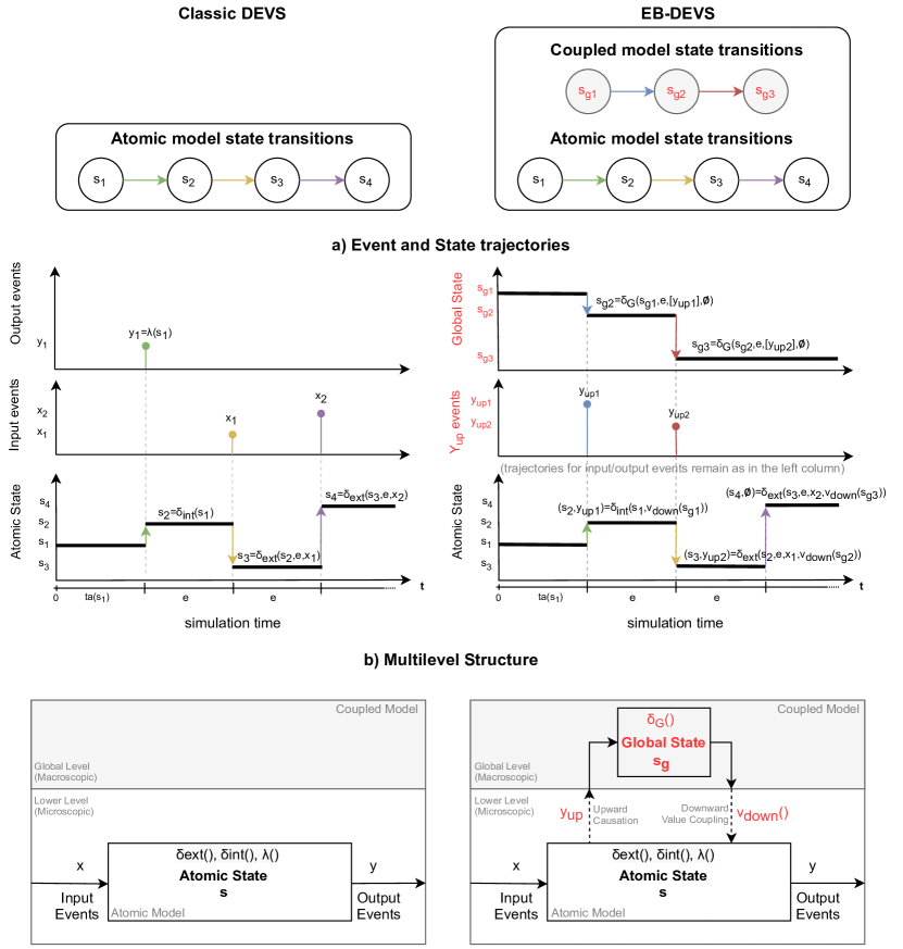
Figure 1: A minimalist example of a Classic DEVS model (left column) and its extension into a an EB-DEVS model (right column) showing the new structure and functions involved and a possible global state trajectory and associated state transition diagrams. The example is meant to capture the simplest hierarchical/modular construct conceived in DEVS, i.e. a single coupled model containing a single atomic model.

2.3.2 A minimalist EB-DEVS extension

Consider an extension of the previous Classic DEVS model now using the EB-DEVS structure. The atomic model $m_{1}$ now belongs to the $C_{1}$ EB-DEVS coupled model that includes the downward information and upward causation mechanisms involving the $\delta_{G}$ and $v_{down}$ functions. We show a simple example with only two levels and one atomic model to introduce the reader with the execution process, more elaborated examples will be displayed in section 3.

To begin with, the internal transition of model $m_{1}$ will execute at time $ta(s_{1})$ as before. To do so, it may also take into account the macro-level information $v_{down}(s_{G1})$ using the downward information channel. The internal transition $(s_{2},y_{up1})=\delta_{int}(s_{1},v_{down}(s_{g1}))$ changes the state of model $m_{1}$ to $s_{2}$ and triggers an upward causation event by sending a $y_{up1}$ value. This causes an invocation of the $\delta_{G}$ function, changing the coupled model’s macro-level state to $s_{g2}=\delta_{G}(s_{g1},e,[y_{up1}],\emptyset)$. The $\delta_{G}$ transition parent’s macro-state value is $\emptyset$ as there are only two levels in this model. Furthermore, in the example there is only one atomic model thus only one upward causation event will be gathered (characterised with a set of $y_{up1}$ values), but the mailbox collects (potentially) multiple upward causation messages.

When $m_{1}$ receives the input event $x_{1}$, it takes into account the macro-level state provided by $v_{down}(s_{g2})$ and transitions into the new state $(s_{3},y_{up2})=\delta_{ext}(s_{2},e,x_{1},v_{down}(s_{g2}))$. This state change triggers a new $\delta_{G}$ transition in $C_{1}$ generating a new macro-level state $s_{g2}=\delta_{G}(s_{g1},e,[y_{up1}],\emptyset)$.

Finally, the atomic model receives a new input message $x_{2}$, this time the model will not generate any $y_{up}$ message and therefore the coupled model will remain in its previous global state $s_{g3}$.

2.4 Relevant features of Complex Systems from the perspective of Emergent Behaviour modelling

In the modelling of complex systems we identified the need for a systematic and reproducible approach to the identification and incorporation of emergent properties. This need is based on the fact that emergent properties are a common denominator in complex systems involving two or more levels of hierarchy. The introduction of new tools that allow the integration of multiple levels of analysis requires the characterisation of common templates of structural features that relate multiple levels within models.

Complex systems such as the artificial societies reproduced in this manuscript are susceptible to identifying and/or incorporating emergent properties. Therefore, we will focus on typical structural features that we consider key in the modelling of such complex systems with emergent properties.

The subsection converges to Table 1 that synthesises where these features can be found in the example models presented later in section 3.

We will focus on the following structural features: the type of communication structure between the agents, whether the communication channel is explicit or implicit, whether the communication structure is static or dynamic, the types of micro-macro communication channels (top-down information and bottom-up causality), the type of emergence present in the model (weak or strong) and how emergent properties are identified (during the simulation run or a posteriori).

In our opinion, said patterns are often overlooked when designing simulation models, while we consider that a proper identification of such structural features is essential for their clear and correct implementation (helped by clear semantics offered by the modelling formalism of choice).

Therefore, we classify these structural features in five categories, involving relations between agents and modelling levels.

Explicit/Implicit communication structure:

When defining the communication mechanism among agents two main types of channels are often used. Explicit channels are those where a message is sent from the source agent directly to the destination agent. On the other hand, implicit channels can be used for indirect coordination between agents using a stigmergic process (Grassé, 1959), a coordination mechanism among entities that use their shared environment as a medium for indirect communication. A microscopic entity (agent) can explicitly retrieve updated information from a macroscopic entity (environment) upon necessity.

Both communication strategies are important. On the one hand, explicit messaging is a causal mechanism: when a message is sent (cause) a state change can be observed (effect). On the other hand, implicit communication is useful when the conditions for the information sharing process are more complex. For instance, when agents interact upon proximity, or triggered by an environmental condition like the scent of pheromones that ants leave in their trails, we rely on indirect information and coordination mechanisms (a comprehensive analysis of the impact, role and evolution of direct and indirect communication mechanisms in simulation models can be found in Tummolini et al. (2009)).

Explicit channels are built into the DEVS formalism by means of links and input-output ports. EB-DEVS extends the communication structure by adding a downward information channel in the mechanism, thus allowing agents at a lower layer to consume information that is only present at a higher level model and, as a consequence, enabling indirect communication among agents.

Static/Dynamic structure:

Dynamic structure models come in a variety of types. The dynamic aspect may refer to the communication machinery (as mentioned above), to the ability of adding/removing agents from the system, or to change a model’s position in a hierarchy. According to Wainer (2009, p.45), there are three structural change types that can occur on the system dynamics:

1. System level: changing the relationship between higher-level entities, for instance between coupled models.

2. Component level: changing the explicit communication network between lower-level atomic models. This happens at the coupled model level.

3. Subcomponent level: structural changes happen at the atomic level. For instance to stop accepting input events or emitting output events.

In this work, two example models (Preferential attachment (section 3.3) and SIR (section 3.5)) use an implementation of Dyn-DEVS (Uhrmacher, 2001) that allows for system-level and component-level changes.

Downward information/Upward causation:

As for multilevel interactions in a system Campbell (1974) and Emmeche et al. (1997) have discussed how higher levels affect or restrict the course of action of bottom level processes. Downward causation, a term coined by Campbell, reflects how a system at the top-level causally drives changes in systems at bottom levels. Analogously, the downward information mechanism only presents higher-level information to lower-level processes, while this information can be either used or dismissed. Upward causation can be seen as a reciprocal, bottom-up relationship.

EB-DEVS implements upward causation by using $y_{up}$ events. When a lower-level model stores a value in the $y_{up}$ variable, an upward causation event will be triggered at its parent model. As for the downward information channel, lower-level models have access to the macro-level state information through the $v_{down}$ function.

Weak/Strong Emergence:

In this work we adopt the definitions in Szabo and Birdsey (2017, p.4): “weak emergence as being the macro-level behaviour that is a result of micro-level component interactions, and strong emergence as the macro-level feedback or causation on the micro-level”. To represent weak emergence with EB-DEVS we resort to the upward causation mechanism, and to model strong emergence we include the downward channel bringing macro-level information to the micro-level models. This closes the required micro-macro feedback loop allowing for adaptive strong emergence (see Mittal (2013) for a discussion of relations between the DEVS formalism, Emergence, Stigmergy and Complex Adaptive Systems modelling).

Emergence identification:

Emergent properties can be modelled and/or identified. Identification can happen either during the simulation (live identification) or after the simulation has finished (ex-post identification).

In the case of live identification, emergent properties are detected at higher-level entities (such as coupled EB-DEVS models).

EB-DEVS features a macro-level state $s_{G}$ for each coupled model that is key to perform live identification by accessing the variable (or variables) that hold information on components, states and aggregated interactions (this is consistent with the concept of Emergence Behaviour Observer snapshots in Mittal and Rainey (2015)).

Ex-post identification of emergent properties are detected while analysing the results of a simulated model and usually does not intervene in the modelling process, while live identification allows for modelling behaviours that depend on the identified properties.

In Table 1 we synthesise the structural features for each of the models that we develop throughout the rest of the paper. Besides the structural features discussed above there are two salient Properties that we consider worth specifying (also included in Table 1).

Structural Feature	Dissemination of Culture	Segregation	Preferential Attachment	Sugarscape	SIR
Explicit/Implicit communication structure	E	I	E	I/E	E
Static/Dynamic structure	S	S	D	S	D
Downward information/ Upward causation	D+U	D+U	U	D+U	D+U
Weak/Strong Emergence	S	W	W	S	S
Emergence identification	Live	Ex Post	Ex Post	Live	Live
Properties
Macroscopic Level Algorithm	CL	None	PA	Gini index	PA
Topology Type	Lattice / Arbitrary	Lattice	Scale Free	Lattice	Scale Free

Table 1: Models implementing emergent characteristics.

The Macroscopic Level Algorithm refers to the technique used to model macro-level aggregate states. During the implementation of our example models we adopted form simple aggregations and clustering techniques to more complex algorithms like size-biased sampling, Preferential Attachment or Gini index calculation.

The Topology Type refers to the structures defined to communicate sub components within a model. In this work we used three types of communication graphs: lattice, random, and scale-free graphs. The implemented models use an input graph that defines the initial connectivity between input and output ports.

In the next section we present five simulation models involving the aforementioned features and properties, and discuss the modelling of emergent behaviour in the context of EB-DEVS.

3 Modelling Emergent Behaviour in Social Dynamics with EB-DEVS

In this section we describe the models implemented. We provide for each of them a general description followed by an analysis regarding their features related to complex systems and emergent behaviour modelling. For an exemplification of the EB-DEVS implementation of different dynamics we outline the pseudocode for each case (adopting a colour convention to highlight the upward causation and downward information mechanisms, and a syntax similar to that of the Python language). Finally, the experimental results for each case study are presented, including a brief discussion regarding the modelling experience using an emergent behaviour-explicit formalism.

3.1 Dissemination of Culture with strong emergent properties

Axelrod’s model of Dissemination of Culture has attracted considerable attention because of its simple rules and its implications for social dynamics. Its main interest lies in the mechanisms it implements to model cultural assimilation. The model implements two important features: social influence and homophily. A social influence model is expected to converge to a monocultural equilibrium. However, Axelrod’s model presents scenarios in which the system moves away from monocultural towards multicultural equilibrium (Centola et al. (2007)). These scenarios are often determined by the number of features and traits that define each culture.

3.1.1 Model dynamics

Each agent has a state with two variables: a features array and a dictionary with the neighbours’ features arrays. The feature array has $F$ values of cultural traits and each cultural trait is defined in the range of integers $[1,Q]$. The state of agents change as they interact with neighbours (assuming an arbitrary topology). An agent selects a neighbour to mix its culture with. and decides to interact based on its similarity. In this context, similarity is defined as the average number of matching traits (i.e. the number of matching traits divided by $F$). If their similarity is greater than a randomly chosen value, cultural mixing occurs. The process consists of choosing, for each agent, one of the different traits in the set of cultural traits and agreeing on a common value with the neighbour.

This simple model exhibits interesting behaviours and has seen several extensions pursuing different degrees of sophistication (Castellano et al., 2000; Balenzuela et al., 2015; Klemm, 2003). From a modelling perspective, the model presents adaptive behaviour (as opposed to rational behaviour) without central authority.

We show in 1 an implementation of the basic dynamics for the culture diffusion model. We provide the pseudocode for a Classical DEVS atomic model representing an agent within a group of interacting agents contained in a same Classical DEVS coupled model (representing the society as a whole).

⬇

1AgentState:

2 neighbours_cultures = {neighbour_id: culture}

3 self_culture = [randint(1, Q) for x in range(F)]

4

5state = AgentState()

6AgentAtomicInternalTransition():

7 # Get a random neighbour culture from the ones it knows.

8 random_neighbour = random_choice(state.neighbours_cultures.keys())

9 # Find the matching positions in the culture array

10 matching_cultures = get_matching_cultures(random_neighbour)

11 share_culture = False

12 # Toss a coin weighted by the percentage of matching cultures

13 if random() < matching_cultures / F:

14 # Randomly choose a trait that is different for both agents and copy it.

15 non_matching_cultures = get_non_matching_cultures(random_neighbour)

16 random_culture, random_culture_index = random_choice(non_matching_cultures)

17 state.self_culture[random_culture_index] = random_culture

18 share_culture = True

19

20AgentAtomicExternalTransition(neighbour_id, culture):

21 # Update local neighbours information

22 state.neighbours_cultures.update({neighbour_id: culture})

23

24AgentAtomicOutputFunction():

25 # Share agents culture with neighbours.

26 share_with_neighbours(state.self_culture)

27

28AgentAtomicTimeAdvance():

29 # Time advance function, if sharing then share the culture immediately.

30 if share_culture:

31 return 0

32 else:

33 return 1

Listing 1: Pseudocode for the Axelrod’s Dissemination of Culture model in Classic DEVS.

3.1.2 Emergence and adaptive behaviour: A fads and fashion scenario

The capabilities of EB-DEVS become relevant when considering extensions to the standard Axelrod’s model. Let’s examine the case of a Fads and fashion scenario. We provide this extension to show how the micro and macro levels can be integrated.

The concept of fashion can be defined as the cultural trait desired by many but defined by few. We can consider that the fashion for a cultural trait is the most popular value among the agents of the system. Said trait can only be observed from a macroscopic level. When this information is made available to the system it can then influence the evolution of agents’ culture over time.

We extend the original model to include this idea in the following way. At the macroscopic level (coupled model) we include a stochastic variable that yields fashion trait values from the agents’ culture arrays. First, it generates a random value in the range $[1,F]$ and then it selects the $q\in Q$ that is most frequent in the system. This type of event (from now on a fashion cultural mix event) is produced at a rate defined by a parameter. During the internal transition an atomic model (i.e, an agent) will toss a weighted coin ($P=FASHION\_RATE$) to undergo either a fashion cultural mix or a regular cultural mix. At the limit values of FASHION_RATE, the model behaves either as the classic model ($P=0$) or as a fashion doppelganger model ($P=1$).

In 2 we show the pseudocode of the Fads and fashion extension.

⬇

1AgentState:

2 neighbours_cultures = {neighbour_id: culture}

3 self_culture = [randint(1, Q) for x in range(F)]

4

5state = AgentState()

6AgentAtomicInternalTransition():

7 # Get a random neighbour culture.

8 random_neighbour = random_choice(state.neighbours_cultures.keys())

9 # Find the matching positions in the culture array.

10 matching_cultures = get_matching_cultures(random_neighbour)

11 share_culture = False

12 # Toss two weighted coins: first determine if it should do Fads and Fashion, then toss a coin weighted by the percentage of matching cultures. Events are mutually exclusive.

13 do_fashion = random() < FASHION_RATE

14 if not do_fashion and

15 random() < (matching_cultures / F):

16 # Randomly choose a trait that is different for both agents and copy it.

17 non_matching_cultures = get_non_matching_cultures(random_neighbour)

18 random_culture, random_culture_index = random_choice(non_matching_cultures)

19 state.self_culture[random_culture_index] = random_culture

20 share_culture = True

21 else:

22 # Ask the parent model for a fashion cultural trait.

23 feature, fashion = $\color[rgb]{1,0,0}v_{down}(FASHION\_FEATURE)$

24 state.self_culture[feature] = fashion

25 # Upward causation message, triggering $\color[rgb]{1,0,0}\delta_{G}$ transition.

26 $\color[rgb]{0,0,1}y_{up}$ = (state.agent_id, state.culture)

27

28AgentAtomicExternalTransition():

29 # Update local neighbours information.

30 state.neighbours_cultures.update({neighbour_id: culture})

31

32AgentAtomicOutputFunction():

33 # Share agent’s culture with neighbours.

34 share_self_culture_with_neighbours()

35

36AgentAtomicTimeAdvance():

37 # Time advance function, if sharing the state then share the culture immediately.

38 if share_culture:

39 return 0

40 else:

41 return 1

42

43CoupledState:

44 models_cultures = {}

45

46$\color[rgb]{1,0,0}s_{G}$ = CoupledState()

47CoupledGlobalTransition($e_{g}$, $\color[rgb]{0,0,1}x^{b}_{micro}$, $\color[rgb]{1,0,0}s_{Gmacro}$):

48 # Update the global status with the cultures from each model

49 $\color[rgb]{1,0,0}s_{G}$.models_cultures.update($\color[rgb]{0,0,1}x^{b}_{micro}$)

50

51$\color[rgb]{1,0,0}v_{down}$(PROPERTY):

52 if PROPERTY == FASHION_FEATURE:

53 cultures_matrix = $\color[rgb]{1,0,0}s_{G}$.models_cultures.values()

54 # Pick a random cultural trait.

55 randfeature = randint(F)

56 feature = cultures_matrix[:, randfeature]

57 # Get the most frequent trait value.

58 fashion_value = bincount(feature).argmax()

59 return randfeature, fashion_value@

Listing 2: Pseudocode of the Dissemination of Culture model with fads and fashion using EB-DEVS. Micro-macro interactions are highlighted with red for $v_{down}$ and blue for $y_{up}$.

3.1.3 Experimental results and discussion

The experiments in Figure 2 were configured as follows: $F=5$, $Q=\{5,20\}$ and $N=100$. We define $N$ agents as atomic models within a same coupled model. The connectivity network is a 10x10 regular lattice. Each simulation realisation is run for 10000 time units.

The parameters $F$ and $Q$ were selected to show two different scenarios of convergence for the classic model, i.e. with FASHION_RATE=0. The scenario with $F=5$ and $Q=5$ shows the model converging towards a monocultural final state, while the scenario with parameters $F=5$ and $Q=20$ converges towards a multicultural state. This is consistent with the original model where small values of $F$ present monocultural convergence and larger values of $Q$ present multicultural convergence. We want to study how the FASHION_RATE affects the system evolution and convergence.

We swept the FASHION_RATE parameter from 0 to 1 with intervals of 0.25, with 10 realisations per experiment. The plots in Figure 2 show the evolution of the mean number of cultures through time.

In 2(a) we can observe that the experiments converge towards a monocultural system for FASHION_RATE = 0. This, again, is consistent with the original model. Nevertheless, we observe that with FASHION_RATE=1 the model also converges towards a monocultural system although at a faster rate. Furthermore, the scenario is clearly affected by intermediate values of FASHION_RATE = {0.75, 0.5, 0.25} where the system now converges towards multicultural states (with a mean number of cultures in the range of 2 to 3)

Looking at 2(b), we see that the original model (FASHION_RATE = 0) converges to a multicultural system with an average of 36 cultures. Interestingly, for FASHION_RATE = 1 the model converges to a monocultural system and for values of FASHION_RATE = 0.75, 0.5, 0.25 the system converges again to a multicultural system with few cultures.

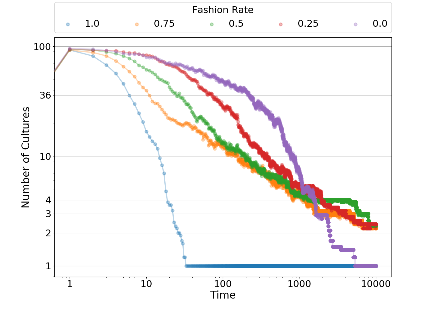
((a)) Dissemination of Culture for F=5, Q=5.

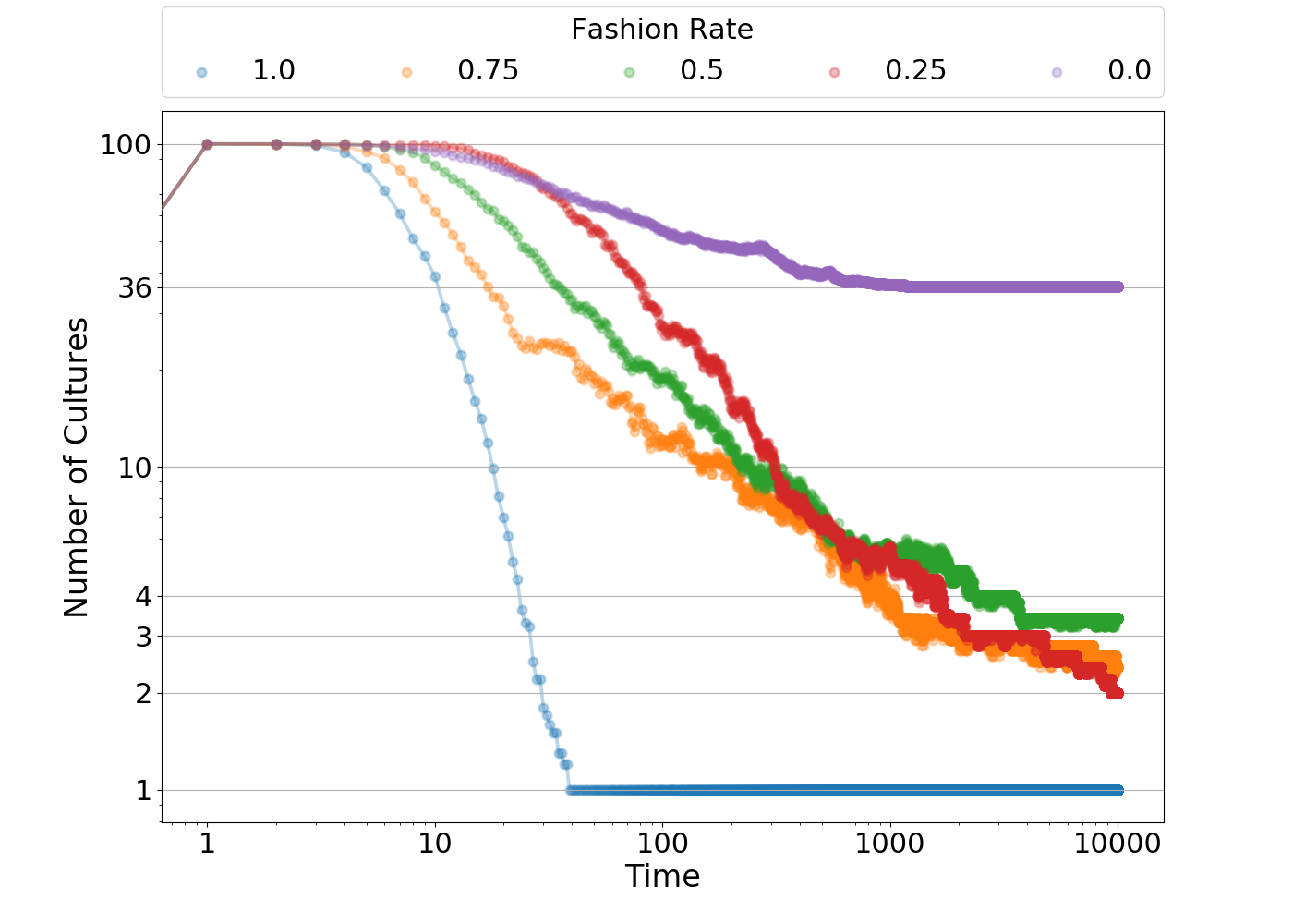
((b)) Dissemination of Culture for F=5, Q=20.

Figure 2: Dissemination of Culture model for 5 cultural features (F), different fashion rates and different numbers of possible cultural traits (Q). The original model (FASHION_RATE = 0, no fashion ever considered) shows a convergence to a monocultural system (left, Q=5) vs. a highly scattered multicultural system (right, Q=20). On the other end (FASHION_RATE = 1, fashion always considered) there is a consistent convergence to monoculture. At intermediate levels of FASHION_RATE the system converges to a slightly scattered multiculture.

The Dissemination of Culture model’s implementation in Classic DEVS is simple. From the modelling perspective, the utilisation of explicit communication channels enables the culture propagation with clear semantics. While the DEVS M&S framework resolves the communication protocol between agents, emergence identification can only be done ex-post, i.e. by analysing the logged time series generated by the experiments.

In Figure 2 we observe a stable macroscopic pattern generated by the agents’ interactions (this observation has been discussed in the computational social sciences field, see Epstein (1999, p.33)). This emergent property cannot be detected at simulation time using Classic DEVS.

The fads and fashion model extends the Axelrod’s basic setting by introducing a micro-macro feedback loop to capture emergent properties. In the model, the system’s overall cultural trend is influenced by the interactions at multiple levels. In the Figure 2 we can see how the fashion rate influences the convergence in two different scenarios. We consider this example as a common pattern for the implementation of strong emergence in simulation models.

Regarding the modelling advantages that EB-DEVS offers for this case study, from an agent’s perspective, the upward causation mechanism ($y_{up}$ messages) allows for a seamless integration with macroscopic variables, while the downward information mechanism makes available required macroscopic information demanding very few changes ($v_{down}$ function). EB-DEVS facilitated the inclusion of emergent properties in an expressive and uncomplicated manner into the Dissemination of Culture model.

3.2 Implicit communication and weak emergence in the Segregation model

In the 70s Thomas Schelling proposed an agent based model to analyse racial segregation (Schelling, 1971). In the model agents are assigned with a colour and an initial position on a grid, where they move according to their happiness evaluated as a function of the colours found in the agent’s neighbourhood. If an agent is surrounded by neighbours of different colour exceeding a given threshold, then the agent is considered unhappy and moves to a random empty position in the grid. Each agent will change its position with a constant time step until it reaches a happy state. The simulation converges to a steady state when all the agents are happy, otherwise the simulation continues forever. Schelling used this model to study the formation of areas segregated by the colour of the skin or race of their population Schelling (1971, p.145).

3.2.1 Model dynamics

We model agents as EB-DEVS atomic models with a state defined by two variables: a colour and a position in the grid, which are randomly selected at the beginning of each simulation. Agents are contained by a single EB-DEVS coupled model that manages the grid representing the environment. In particular, the coupled model provides the atomic models with macro-level information such as an available free position where to move or the number of neighbours matching the agent’s colour.

Agents do not know about the grid nor the number of agents (the size of the system). Therefore, they resort to the macro-level information to calculate their happiness relative to the neighbours colours. In the case of an unhappy result they move to a random empty cell, which is also provided by the coupled model. We utilised the upward causation and downward information capabilities of EB-DEVS for the implementation of indirect communication.The upward causation event $y_{up}$, triggers the global transition function $\delta_{G}$ updating the colours in the grid, and the $v_{down}$ function provides a (partially) macroscopic information about the happiness of neighbouring agents.

The model has the following parameters: the size of the grid, the number of agents, and the happiness threshold. In 3 we show the pseudocode of the model.

⬇

1AgentState:

2 # Initial agent’s state

3 colour = get_random_colour(RED, GREEN)

4 position = get_initial_position()

5

6state = AgentState()

7AgentAtomicInternalTransition():

8 # Get information from the parent model regarding its happiness relative to its neighbours.

9 happy = $\color[rgb]{1,0,0}v_{down}$(HAPPINESS, state.position, state.colour)

10 last_pos = state.position

11 if not happy:

12 # Unhappy agents move to a random empty position defined by the parent model.

13 empty_cell = $\color[rgb]{1,0,0}v_{down}$(RANDOM_EMPTY_CELL)

14 state.position = empty_cell

15 $\color[rgb]{0,0,1}y_{up}$ = (last_pos, state.position)

16

17AgentAtomicTimeAdvance():

18 # Sampled time from the exponential distribution.

19 return random_exponential(0.5)

20

21CoupledState:

22 # Initial global state of each agent at each position in the grid

23 grid = GRID(20,20)

24

25$\color[rgb]{1,0,0}s_{G}$ = CoupledState()

26CoupledGlobalTransition($e_{g}$, $\color[rgb]{0,0,1}x^{b}_{micro}$, $\color[rgb]{1,0,0}s_{Gmacro}$):

27 # Update the grid position value of each agent communicating its new colour.

28 for last_pos, actual_pos in $\color[rgb]{0,0,1}x^{b}_{micro}$:

29 colour_swap = $\color[rgb]{1,0,0}s_{G}$.grid[last_pos]

30 $\color[rgb]{1,0,0}s_{G}$.grid[last_pos] = EMPTY

31 $\color[rgb]{1,0,0}s_{G}$.grid[actual_pos] = colour_swap

32

33$\color[rgb]{1,0,0}v_{down}$(PROPERTY, parameters):

34 # Value Coupling function that communicates a random empty cell and relative happiness value.

35 if PROPERTY == RANDOM_EMPTY_CELL:

36 return random_empty_cell()

37 elif PROPERTY == HAPPINESS:

38 return happiness_from_neighbours(parameters.position, parameters.colour)

Listing 3: Pseudocode of the Schelling’s segregation model. Micro-macro interactions are highlighted in red for $v_{down}$ and blue for $y_{up}$ and $x^{b}_{micro}$.

3.2.2 Adaptive behaviour and implicit communication

The implementation of the model presents relevant features from the modelling standpoint. The environment (coupled model) maintains an updated state of the occupancy on the grid, enabling the implementation of implicit communication for proximity-based interactions between agents. This allows to share the happiness and the available positions in the grid with the agents without the need of explicit links between atomic models.

Combining static structures (i.e., the grid) with implicit communication mechanisms enables macroscopic-driven adaptive behaviour at the microscopic-level. Furthermore, this short example provides the basis for weak emergence modelling.

3.2.3 Experimental results and discussion

In Figure 3 we can see the simulation results for the model. The experiments were done for two different population sizes, N={266, 200}. The Happiness Threshold was swept for the values HT = {0.20, 0.35, 0.50, 0.65, 0.80, 0.95}. The size of the grid is 20x20 cells and the experiments were configured for a duration of 40 units of time, performing 10 realisations for each combination of parameters.

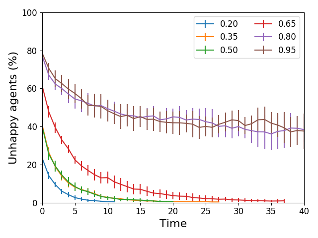
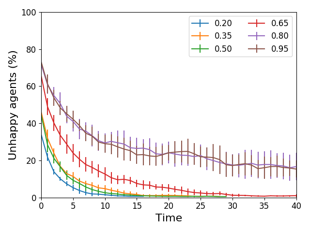
Figure 3: Simulation and modelling of the Schelling’s segregation model. Scenarios varying happiness thresholds were simulated for with two different populations: left) 266 agents and right) 200 agents.

The system converges when the number of unhappy agents drops to zero. In the cases where the system converges, ghettos appear in the grid as clusters of agents sharing the same colour. System’s convergence depends mainly on the size of the system and the happiness threshold. This can be seen analysing the percentage of unhappy agents as a function of time (Figure 3). The cases where the system does not converge to zero unhappy (HT = {0.8, 0.95}) were cut off at 40 time units.

In this example, we have used implicit communication with static structure. The downward and upward mechanisms, are used for the implementation of indirect communication of the neighbouring happiness values. This implementation reduces the model’s complexity in two ways. On the one hand, it reduces the number of input/output explicit links (with all their associated DEVS message handling overhead) that would otherwise have been required. On the other hand, it allows to update the agents’ (implicit) communication structure in an easy way (avoiding to rewire a classic explicit DEVS structure, which requires more sophisticated considerations and mechanisms such as dynamic structure capabilities (Uhrmacher (2001)).

Finally, we remark that this model exhibits a weak form of emergence, presenting a stable macroscopic pattern allowing only for ex-post emergence identification. It could be possible to extend the model by incorporating strong emergence, which can be considered in a future work.

3.3 Dynamic explicit networks in the Preferential Attachment model

The scale-free property (Albert and Barabási, 2002) appears in many complex networks of agents describing social interactions and collaborations, biological relations, the World Wide Web, financial and payment networks, semantics, airlines, just to name a few. The degree of interconnection between agents, i.e.: the degree of each node in the connectivity graph, in these large networks follows a power law distribution, which seems to be a consequence of the expansion of the network following a Preferential Attachment (PA) process (Albert and Barabási, 2002, p. 76). Namely, each newly added node is more likely to connect with existing nodes with high degree. Eventually as the system evolves, the nodes start forming hubs that exhibit a power-law distribution in the degree of the nodes. This macroscopic structure originates from microscopic rules of connectivity, and is presented as a form of emergent property of the system.

3.3.1 Model dynamics

In order to simulate the Preferential Attachment process in EB-DEVS, we will model the evolving graph as nodes (represented by agents) that attach to the existing network.

We consider an initial graph with two nodes connected by an edge, where each node is implemented as an EB-DEVS atomic model, and edges are explicit links connecting input output ports. At each step of the simulation a new node is added to the network, and is connected with $n$ of the previously existing nodes, which are selected using a random variable sampled from a size-biased distribution, modelled using the coupled model’s macro-level state. Therefore, the probability to select a neighbour of degree $k$ is ${(k.p_{k})}/{\sum_{j=1,...,n}(j.p_{j})}$ where $p_{k}$ is the proportion of existing nodes with degree $k$. Following this property, the probability of a node to be chosen is proportional to its degree, making the higher-degree nodes prone to gain more neighbours. Furthermore, older nodes will correlate with hubs.

A network that evolves following these rules will be composed of nodes whose degree have a scale-free distribution (Albert and Barabási, 2002). The probability $p_{k}$ that a vertex in the network has degree $k$ follows a power-law distribution. Namely, $p_{k}$ is proportional to $k^{-\gamma}$ for some $\gamma$.

3.3.2 Scale-free network generation and adaptive behaviour

The implementation of this model presents several modelling challenges that we consider of interest. As the model requires to dynamically add new atomic components and links, we face a case of dynamic structure in the context of EB-DEVS. Dynamic structure models enable the expression of more complex systems as we will see in section 3.5. Secondly, our preferential attachment implementation resorts to upward causation and weak emergence to drive the evolution of the dynamic structure network. This allows for the emergence of a higher-level structure as it was previously described. This example shows how dynamic networks with explicit links can be built with EB-DEVS in a compact and sound way.

In 4 we show the pseudocode of the Preferential Attachment model.

⬇

1AgentState:

2 id = incremental id

3 outdegree = 0

4

5state = AgentState()

6NodeAtomicInternalTransition():

7 # Triggers an upward causation event towards the coupled model carrying its out degree.

8 $\color[rgb]{1,0,0}y_{up}$ = (id, outdegree)

9

10CoupledState:

11 # Model’s initial topology

12 topology = Parameters.INITIAL_TOPOLOGY

13 # Model’s state with nodes degrees

14 nodes_degree = {}

15

16$\color[rgb]{1,0,0}s_{G}$ = CoupledState()

17CoupledGlobalTransition($e_{g}$, $\color[rgb]{0,0,1}x^{b}_{micro}$, $\color[rgb]{1,0,0}s_{Gmacro}$):

18 # Updates the macro level state with the agent’s out degree

19 for elem in $\color[rgb]{0,0,1}x^{b}_{micro}$:

20 nodes_degree[elem.id] = elem.outdegree

21 # Defines the dynamic network behaviour:

22 # Retrieve the node’s degree sequence

23 degree_sequence = nodes_degree.values()

24 # Create size-biased probability array

25 pk = [degree / sum(degree_sequence) for degree in degree_sequence]

26 # Sample from the weighted distribution the nodes to connect to

27 connect_to_node = choice(nodes_degree.keys(), pk, replace=False, number=Parameters.CONNECT_TO)

28 atomic = create_atomic_model()

29 # Create, connect and update topology

30 for node in connect_to_node:

31 connect_models(atomic, node)

32 update_topology()

Listing 4: Pseudocode of the Preferential Attachment model. Micro-macro interactions are highlighted with red for $v_{down}$ and blue for $y_{up}$ and $x^{b}_{micro}$.

3.3.3 Experimental results and discussion

The experiments in Figure 4, were done for a virtual time of 10000 units. The generated network presents 10000 connected nodes. Three experiments were done using different values of the CONNECT_TO parameter for 10 realisations each. Every node connects to either one, two or three existing nodes sorted from the size-biased distribution.

In 4(a), 4(b) and 4(c) we show the final degree distribution of the nodes in the network. In blue we provide the curve fitting of the corresponding power-law distribution. Additionally, 4(d) shows the time evolution of the network’s average degree for all the experiments.

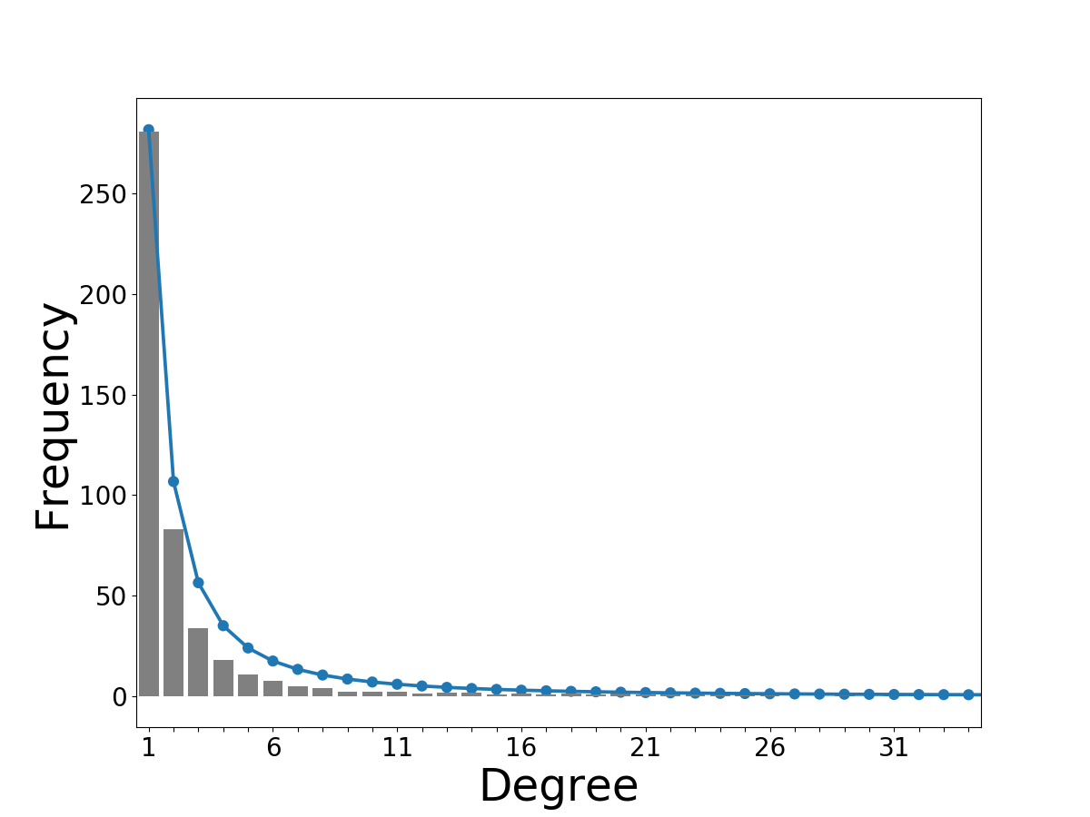
((a)) Connect to one node.

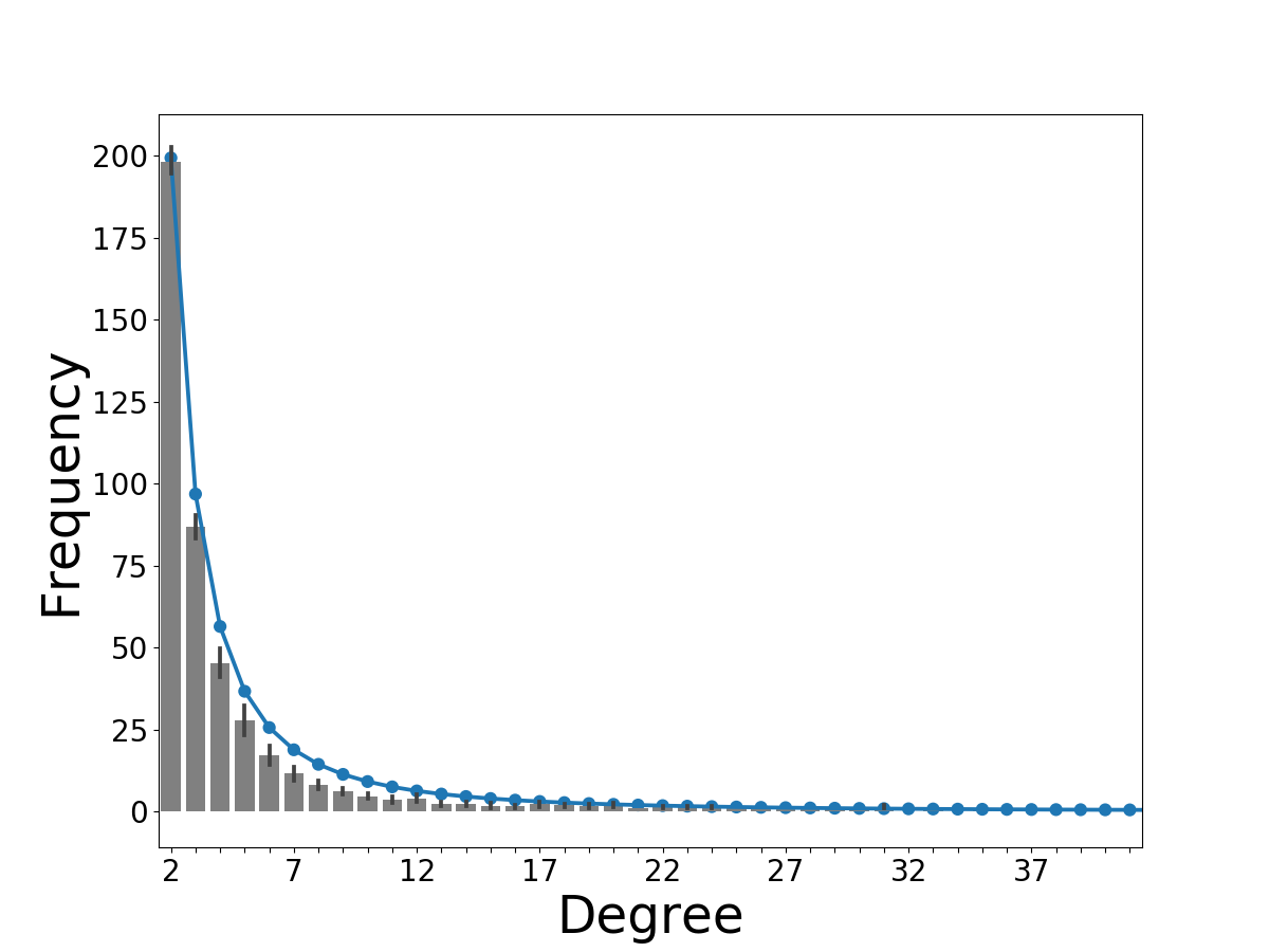
((b)) Connect to two nodes.

((c)) Connect to three nodes.

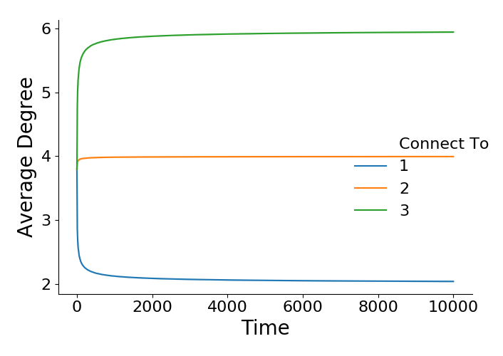
((d)) Average degree evolution for the three submodels.

Figure 4: Preferential Attachment model with three connectivity strategies.

The canonical PA model describes how some particular explicit dynamic structures evolve through time. During the implementation of this example, it was possible to analyse the impact of upward causation in the implementation of dynamic structures based on macro-level variables. The model shows an emergent pattern that can be analysed either live (if an atomic model would require so) or, as we show in this brief example, after the simulation execution. In this sense the PA model exhibits weak emergence through the upward causation mechanism. Moreover, when designing agents that consume macro-level topology aggregated variables, it is possible to exhibit strong emergent properties.

Finally, the PA is a simple model to implement in EB-DEVS that functions as a template for the development of complex models that require a dynamic and explicit communication topology. We will extend the SIR model in section 3.5 to show the advantages and power of this approach.

3.4 Model heterogeneity and strong emergence in the Sugarscape model

In the 90s Joshua M. Epstein and Robert Axtell presented the Sugarscape model (Epstein and Axtell, 2018) to analyse wealth distribution in a grid of moving agents. As Schelling’s model, agents move in a grid according to some rules. In this case, positions in the grid have a resource that agents consume (e.g.: sugar). Every time an agent moves, it looks for the position with the maximum amount of sugar within its range of vision, consumes all the sugar in that place and adds it up to its wealth. Immediately after, the agent consumes its wealth at a certain metabolic rate. If its wealth reaches zero after this consumption the agent dies.

The age of an agent increases steadily, eventually leading to its death when a maximum value (randomly defined for each agent) is reached. When an agent dies, another agent is created at a random position (with random parameters, see below).

Resources are distributed in the grid and regenerate at a rate of 1 unit per time unit. Each cell has a maximum capacity and sugar regenerates until the cell is full.

3.4.1 Model dynamics

The model has several parameters defining the agents’ properties: the range of vision, metabolic rate, maximum age, and initial wealth. The agents have a state defined by their age, wealth, and their positions in the grid. The initial state is selected randomly using a uniform distribution between values defined by the model parameters. Furthermore, when an agents dies the new agent is assigned with new random values.

The grid has another set of parameters: the number of cells, the dimensions, and the maximum capacity distribution. This parameters define the simulated terrain. In the original Sugarscape model the grid was developed to have two regions with high maximum capacity, connected by a valley of middle capacity, and surrounded by a desert of zero capacity. We use this very same terrain definition.

It is well known that the network topology influences the dynamics of the simulated model. Agents would prefer to move to positions with higher sugar availability, while positions with lower sugar availability would be statistically avoided.

For the implementation of this model we considered that the time step for resource’s regeneration and consumption should be independent. This motivates the two types of atomic models present in the model, the Agents and the Cells.

3.4.2 Emergence and adaptive behaviour in the Sugarscape model

In the pseudocode of 5 we present the Sugarscape model extended to include strong emergent properties. This new model makes use of a macro-level property: the Gini index, a statistical dispersion metric that is widely used to measure wealth inequality. This value is calculated at the coupled model, and its updates are triggered by the upward causation mechanism.

We extend the agent behaviour to use this information via the downward information mechanism. Each time an agent moves to a new position, and before consuming the available sugar, it queries the environment for the Gini index variable. If the Gini index is below a certain threshold, then the agent performs its regular consumption behaviour. Otherwise, if the Gini index is above the threshold (wealth is not enough equally distributed) then the agent performs a less aggressive behaviour, consuming only an amount of sugar enough to match the demand of its metabolic rate.

The remaining features and rules of the model remains the same.

In 5 we present the model’s pseudocode.

⬇

1AgentState:

2 # Initial agent values

3 position = (randint(0,30), randint(0,30))

4 vision = random(1,6)

5 metabolic_rate = random(1,2)

6 wealth = random(5,25)

7 max_age = random(5,25)

8 age = 0

9 last_consumed = 0

10

11state = AgentState()

12AgentAtomicInternalTransition():

13 last_position = state.position

14 # Get highest sugar cell from parent

15 cell_pos, cell_sugar = $\color[rgb]{1,0,0}v_{down}$(MAX_SUGAR_NEXT_CELL, state.position, state.vision)

16 state.position = cell_pos

17 # Get macro-level variable, Gini index

18 gini_coef = $\color[rgb]{1,0,0}v_{down}$(GINI)

19 if gini_coef < GINI_CUTOFF:

20 # Regular Sugarscape behaviour

21 state.last_consumed+= cell_sugar

22 else:

23 # If there is inequality, consume as little as metabolic_rate

24 state.last_consumed+= min(cell_sugar, state.metabolic_rate)

25

26 # Update agent state

27 state.wealth+= state.last_consumed

28 state.wealth-= state.metabolic_rate

29 state.age+= elapsed_time

30 # If the agent has no wealth or is too old, die

31 if state.wealth < 0 or age > max_age:

32 die()

33 # Trigger the upward causation event with the agent’s new state information

34 $\color[rgb]{0,0,1}y_{up}$ = (AGENT, last_position, state.position)

35

36AgentAtomicOutputFunction():

37 # Consume the cell position sugar, informing the CellAtomic it was consumed

38 dict_consumed_position = {state.position : self.last_consumed}

39 return dict_consumed_position

40

41AgentAtomicTimeAdvance():

42 # Sample time for the next internal transition from the distribution (if the agent is alive). Otherwise it will not transition anymore.

43 return random_exponential(0.5) if state.alive else INFINITY

44

45CellState:

46 # Cell initial values based on the distribution of grid’s capacity values.

47 position = INIT_VALUE_pos

48 growth_rate = INIT_VALUE_gr

49 sugar = INIT_VALUE_sg

50 max_capacity = INIT_VALUE_mc

51

52CellAtomicExternalTransition(consume):

53 # Discount the consumed sugar

54 state.sugar-= consume

55

56CellAtomicInternalTransition():

57 # Regenerate the sugar during the internal transition

58 state.sugar+= 1

59 $\color[rgb]{0,0,1}y_{up}$ = (CELL, state.position, state.sugar)

60

61CellAtomicTimeAdvance():

62 return random_exponential(0.5)

63

64CoupledState:

65 # Define the grid and the number of agents on the system

66 grid = GRID(30,30)

67 # Create 50 agents.

68 init_agents(50)

69

70CoupledGlobalTransition($e_{g}$, $\color[rgb]{0,0,1}x^{b}_{micro}$, $\color[rgb]{1,0,0}s_{Gmacro}$):

71 # Update macro-level state using agent’s and cell’s informed values

72 for x in $\color[rgb]{0,0,1}x^{b}_{micro}$:

73 # If the information comes from an Agent model

74 if x[0] == AGENT:

75 last_pos = x[1]

76 actual_pos = x[2]

77 # Move the agent from the last know position to the new position if and only if the agent is alive

78 $\color[rgb]{1,0,0}s_{G}$.agent_grid[last_pos] = EMPTY

79 $\color[rgb]{1,0,0}s_{G}$.agent_grid[actual_pos] = OCCUPIED if x[3] else DEAD@

80 elif x[0] == CELL:

81 # If the information comes from a Cell model

82 # Update the cell’s available sugar

83 pos = x[1]

84 sugar = x[2]

85 $\color[rgb]{1,0,0}s_{G}$.sugar_grid[pos] = sugar@

86

87$\color[rgb]{1,0,0}v_{down}$(PROPERTY, parameters):

88 # Downward information function

89 if PROPERTY == MAX_SUGAR_NEXT_CELL:

90 # Return the cell with maximum sugar

91 return get_sugar_cell(parameters.position, parameters.vision)

92 if PROPERTY == GINI:

93 # Return the Gini index based on the agents’ wealth

94 return Gini([ ag.wealth for ag in agents ])

Listing 5: Pseudocode of the Epstein’s sugarscape model. Micro-macro interactions are highlighted with red for $v_{down}$ and blue for $y_{up}$ and $x^{b}_{micro}$.

3.4.3 Experimental results and discussion

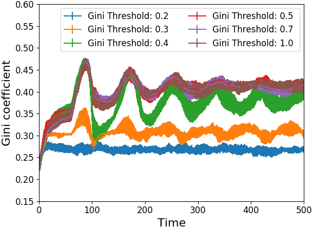
Figure 5: Simulation and modelling of the Epstein’s Sugarscape model. Scenarios varying Gini cutoff.

As it can be seen in Figure 5, we swept the Gini threshold to analyse the effect in the wealth distribution. The classic behaviour can be appreciated when the Gini threshold is equal to 1. In this case, the Gini index starts around 0.22, and it oscillates through time until it reaches a stable value of 0.42. The initial value depends on the first randomly assigned values of wealth. The final value depends on these values, but also is heavily dependant on the grid topology. This is also noted by Epstein and Axtell. In addition, when we run the simulations using thresholds of 0.4 or below, the Gini index oscillates and stabilises around a wealth distribution equal to the Gini threshold. Finally, if we set the threshold to 0.2 the agents behave less aggressively. In this case, the Gini index does not oscillate, reaching a final value of 0.27. Higher values of the Gini threshold don’t affect the system’s convergence.

In this example several complex systems’ features are present. In particular, we would like to highlight how explicit and implicit communication structures can coexist.

Explicit communication channels were used between the agents and the cells. This allows the agents to signal sugar consumption, causing the cell to update its stock. This strategy facilitates the modelling by using the Separation of Concerns (SoC) principle (coined by Dijkstra (1982)) which simplifies the design of complex processes by means of modularization.

Additionally, indirect communication was used to communicate to the agents the available sugar in the grid. In this regard, we observe great flexibility in two aspects. Firstly, the information on resources’ availability is shared through the environment using stigmergy to coordinate the agents. Secondly, macro-level variables such as the Gini index are integrated with ease into the model providing for a rich extension with minimal changes. For the extension is vital the role that plays upward causation for the calculation of the aggregated information and downward information by making available such information.

Finally, we remark that the model presents strong emergence, relating the micro and macro levels. The closed feedback loop uses the Gini index as a macro-level state feeding the micro level models with information that prevents the wealth accumulation. This can be observed in the model’s dynamics where lower values of the Gini threshold parameter influences the average wealth distribution of the population. For higher threshold values, the system is less influenced, behaving more as the original Sugarscape model.

3.5 A dynamic network SIR model using a Preferential Attachment contact process

SIR models are now very famous, a finite population is divided in three compartments or states: Susceptible, Infected and Recovered. Individuals in the first state may contract a disease and transition to the Infected state, where they propagate the illness to potential contacts. After an infection period, agents go to Recovered state and remain in it forever.

We simulate an epidemic contact process taking place over a Configuration Model random graph where agents can be in three possible states: Susceptible, Infected and Recovered. The total number of Susceptible, Infected and Recovered nodes over time is denoted $S_{t},I_{t}$ and $R_{t}$ respectively.

The model resorts to the so called principle of deferred decisions (Mitzenmacher and Upfal, 2005), revealing the graph simultaneously with the propagation of the disease. Succinctly, the configuration model graph is dynamically generated as the infection spreads through the model’s nodes. The generation of the graph follows a Preferential Attachment (PA) process with different parameters than the ones discussed in section 3.3.

3.5.1 Configuration model graph

The selected dynamic communication structure (stochastic environment) is the Configuration Model (CM), a class of random graph introduced in Bollobás (1998). It can be constructed as follows:

Define the sequence of degrees $s=k_{1},\dots,k_{n}$ for nodes $i\in[1,n]$, to be independent and identically distributed according to $p^{(n)}=(p^{(n)}_{k})_{k=1,...,n}$. Following $p^{(n)}$, generate a list of half-edges for each $k_{i}$. To generate the nodes degree sequence, select two random nodes with unmatched half-edges and connect them, remove those half-edges and continue selecting nodes until there are no more available nodes with unmatched half-edges.

The result of this procedure is a graph with a node degree sequence distributed according to $p^{n}$, and the probability that a neighbour has degree $k$ is $\frac{kp_{k}}{\sum_{j=1,...,n}jp_{j}}$, which is the size-biased degree distribution. This distribution will greatly influence the dynamics on CM models as opposed to the mean field point of view, where the underlying graph of potential connections is complete.

3.5.2 Model dynamics

We first introduce a stochastic description of the model’s dynamics, later we give the ordinary differential equations of the model, and finally we describe the EB-DEVS implementation.

For a given Susceptible node we consider multiple exponential clocks with parameter $\beta$ one for each edge connecting it with an Infected node. This represents the potential encounters. When either clock rings, the Susceptible transitions into the Infected state and remains infectious for an exponential time with mean $1/\gamma$. When this clock rings, it changes its state to Recovered preventing future infections.

Now let us introduce the differential equation model that describes the SIR dynamics in random networks with heterogeneous connectivity (Decreusefond et al., 2012; Volz, 2008).

First consider that $p^{X}$ denotes the probability that an edge connects a Susceptible with a node in state $X$, for $X=S$, $I$ or $R$. Second, consider the probability generating function $g$ of the initial degree of agents. Finally, consider the probability $\alpha$ of a node of degree one to remain Susceptible at time t. This system strongly depends on $g$ and $\alpha$.

$$\left\{\begin{array}[]{l}\dot{\alpha}=-\beta p^{I}\alpha\\ \dot{I}=-\gamma I+\beta p^{I}\alpha g^{\prime}(\alpha)\\ \dot{p^{S}}=-\frac{\alpha g^{\prime\prime}(\alpha)}{g^{\prime}(\alpha)}p^{S}\beta p^{I}+p^{S}\beta p^{I}\\ \dot{p^{I}}=-\gamma p^{I}+p^{I}rp^{S}\frac{\alpha g^{\prime\prime}(\alpha)}{g^{\prime}(\alpha)}-rp^{I}(1-p^{I})\\ \end{array}\right.$$ (5)

where $\beta$ and $\gamma$ are the contagion and recovery rates, respectively.

The implemented EB-DEVS model translates the stochastic process in the following manner:

• The agents have a state defining the compartment they belong to, the neighbours’ state, and the free degree available for new connections (or available half-edges).

• Initially, all agents are Susceptible except for a seed agent in Infected state. The Infected agent is connected to a set of randomly selected Susceptible agents.

• Agents change their state to Infected upon reception of the ’infect’ message. This is defined in the external transition function. If an agent gets Infected, it will share its new state with the connected (neighbouring) agents. When an agent changes its state to Infected, the state change triggers an upward causation event generating a structural change.

• The output function, which is invoked with each internal transition, emits values to infect agents and to propagate its state when it changes. An Infected agent will either infect or recover with a probability proportional to the number of Susceptible neighbours.

• The atomic time advance function defines the exponential clocks for each state (Susceptible, Infected or Recovered). In the case of Infected agents, we resort to the exponential race formula (Bocharov et al., 2011, lemmas 1.2.2 and 1.2.3) to trigger the time advance on the first exponential clock. The formula is adjusted for the number of Susceptible agents in that particular moment.

• The coupled model drives the dynamic structure changes that connects the newly Infected agent to other agents using the size-biased distribution.

3.5.3 Emergence and adaptive behaviour in the social isolation scenario

We extend the SIR model previously discussed to highlight the strengths of the EB-DEVS approach.

To do so, we define two variables that control if agents isolate from the sources of infection or behave as previously defined. The Quarantine Threshold (QT) models when the system enters a quarantined state, and the Quarantine Acceptance (QA) models the acceptance of the social isolation policy (enforced by the environment).

Regarding the QT parameter, if the percentage of the infected population reaches QT, the macro-level state QUARANTINE_CONDITION is activated. If this condition is met, the agents throw a weighted coin with probability equal to the QA parameter. If the agent accepts the isolation, it prevents the infection by discarding any infect message received.

This mimics the process of social isolation during an epidemics’ outbreak.

In 6 we present the pseudocode of the complete model.

⬇

1AgentState:

2 id = incremental id

3 # Define the initial state for each agent. There is only one infected agent at the beginning of the simulation.

4 state = Susceptible if id!=0 else Infected

5 neighbours_state = {}

6 free_degree = random_poisson(lambda)

7

8state = AgentState()

9AgentAtomicInternalTransition():

10 # State change into Recovered

11 if state == Infected and to_recover:

12 state = Recovered

13 share_state()

14 ta = INFINITY

15 else:

16 # Restart to_recover and infect exponential clocks

17 set_infection_values()

18 # Upward causation message to sync the agent state with the coupled model

19 not_new_infected = False

20 $\color[rgb]{0,0,1}y_{up}$ = (state.id, state.outdegree, not_new_infected)

21

22AgentAtomicExternalTransition(message):

23 share_state = False

24 new_infected = False

25 # If received an infect message and is Susceptible, get infected

26 quarantine_accept = random() < QUARANTINE_ACCEPTANCE

27 if message == ’infect’:

28 do_quarantine = $\color[rgb]{1,0,0}v_{down}$(QUARANTINE_CONDITION)

29 if state == Susceptible and (not do_quarantine or quarantine_accept):

30 state = Infected

31 share_state = True

32 state.model_transition = True

33 new_infected = True

34 else:

35 # Update the neighbours known state

36 update_neighbours_state()

37 # Upward causation message to sync the agent state with the coupled model

38 $\color[rgb]{0,0,1}y_{up}$ = (state.id, state.outdegree, new_infected)

39

40AgentAtomicTimeAdvance():

41 # Time advance for the infected agent

42 if state == Infected:

43 if any(susceptible_neighbours):

44 # If there are any susceptible neighbours

45 prob = RHO_PROB / (number_of_susceptible_neighbours * BETA_PROB + Parameters.RHO_PROB)

46 to_recover = random() < prob

47 ta = random_exponential(1/(number_of_susceptible_neighbours * BETA_PROB + RHO_PROB))

48 else:

49 to_recover = True

50 ta = random_exponential(1/RHO_PROB)

51 # If the mode is not infected it will wait indefinitely

52 elif state == Susceptible or state == Recovered:

53 ta = INFINITY

54

55AgentAtomicOutputFunction():

56 ret = {}

57 # If sharing its own state, share it with all the neighboring models

58 if state.share:

59 for outport in self.OPorts:

60 ret[outport] = (state.id, state.state)

61 return ret

62 # If Infected and not recovering, send an infect message

63 if self.state.state == SIRStates.I and self.state.to_recover == False:

64 # Ignore the case where there are no neighboring agents

65 if len(self.OPorts) == 0:

66 return

67 susceptible_ids = state.susceptible_neighbors_ids

68 if susceptible_ids == None:

69 return

70 # Randomly choose one susceptible neighbor

71 outmodel_id = random_choice(susceptible_ids)

72 outport = get_outport(from=state.id, to=outmodel_id)

73 if outport != None:

74 ret = {outport[0]: "infect"}

75 return ret

76 return

77

78CoupledState:

79 topology = Parameters.INITIAL_TOPOLOGY

80 nodes_degree = {}

81 agent_states = {}

82

83$\color[rgb]{1,0,0}s_{G}$ = CoupledState()

84CoupledGlobalTransition($e_{g}$, $\color[rgb]{0,0,1}x^{b}_{micro}$, $\color[rgb]{1,0,0}s_{Gmacro}$):

85 # Update the out degree for the node with id=id

86 for id, outdegree, new_infected in $\color[rgb]{0,0,1}x^{b}_{micro}$:

87 nodes_degree[id] = outdegree

88 # If a new infected node, then change the structure

89 if new_infected:

90 # Structure change code section

91 # Generate the probability distribution for nodes connection

92 degree_sequence = nodes_degree.values()

93 pk = [degree / sum(degree_sequence) for degree in degree_sequence]

94 # Pick one with the discrete distribution

95 connect_to_node = choice(nodes_degree.keys(), pk, replace=False, number=Parameters.CONNECT_TO)

96 # Connect the newly_infected to each of the selected nodes (all susceptible)

97 for node in connect_to_node:

98 connect_nodes(id, node)

99 update_topology()

100

101$\color[rgb]{1,0,0}v_{down}$(PROPERTY, parameters):

102 if PROPERTY == ENVProps.QUARANTINE_CONDITION:

103 # count the number of agents per state.

104 (unique, counts) = unique_count($s_{G}$.agent_states)

105 # Filter the infected agents.

106 unique_counts_dict = dict(zip(unique, counts))

107 infected_number = unique_counts_dict[’Infected’]

108 # Calculate the percentage of infected agents.

109 infected_percentage = infected_number / float(len(self.agents))

110 # Return true if the agents should isolate.

111 return QUARANTINE_THRESHOLD < infected_percentage

Listing 6: Pseudocode of the SIR Model including the social isolation scenario. Micro-macro interactions are highlighted with red for $v_{down}$ and blue for $y_{up}$ and $x^{b}_{micro}$.

3.5.4 Experimental results and discussion

In Figure 6 we show how the agent-oriented EB-DEVS model compares to a mean field model (a set of ODEs solved by numerical integration) for the same SIR system.

The experiments were configured for parameters $\gamma=1$, $\beta=3$ and an initial free degree distribution of nodes following a $Poisson(\lambda=8)$. The experiments were run for 4 units of time and 30 realisations.

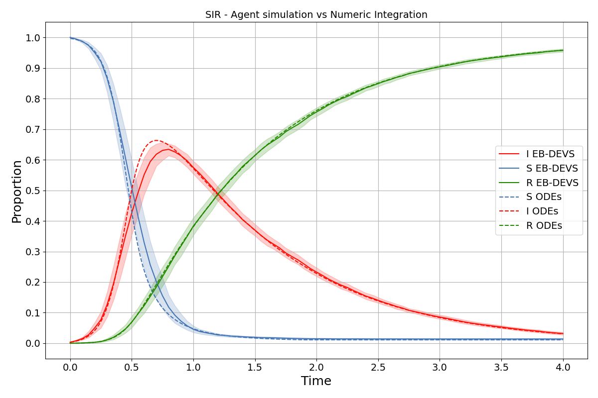
Figure 6: Comparison of SIR dynamics for EB-DEVS simulation (solid line) vs. numerical integration of ODEs (dashed). Parameters: $\gamma=1$, $\beta=3$, $\lambda=8$

We can observe that the EB-DEVS model matches closely the theoretical trajectories of SIR dynamics over a Configuration Model (Decreusefond et al., 2012).

Regarding the social isolation model, we can see from the scenarios evaluated in 7(a) that lower QT values correlate with a reduction in the maximum infected population.

By preventing social contact during the rise of an epidemic outbreak it is theoretically possible to control the simultaneous number of infected agents. This number will depend on the chosen parameters QT and QA. Nevertheless, this strategy shows that in time all agents get infected.

We observe that the QA parameter plays a fundamental role in the evolution of the infected population. As it can be seen in 7(b) the maximum number of infected agents depends not only on the QT parameter, but is also conditioned by QA. Lower QA values match the standard SIR model behaviour, while a higher QA present a behaviour similar to the exhibited in 7(a).

We also observe a plateau in the curve of the infected population in 7(a) which is not characteristic of classical SIR model. Indeed, quarantines can control the peak of epidemics, demonstrating that such strategies can be useful to avoid saturations of the health system.

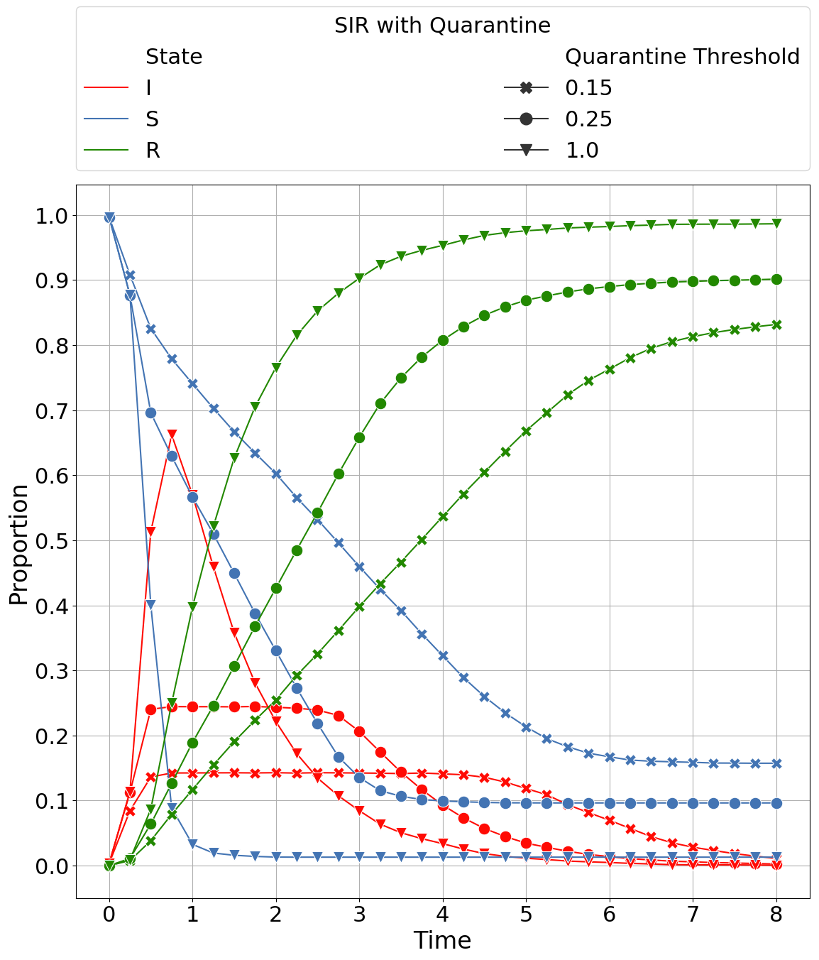
((a)) Quarantine Threshold (QT) sweep. $QA=1,\gamma=1$, $\beta=3,\lambda=8$

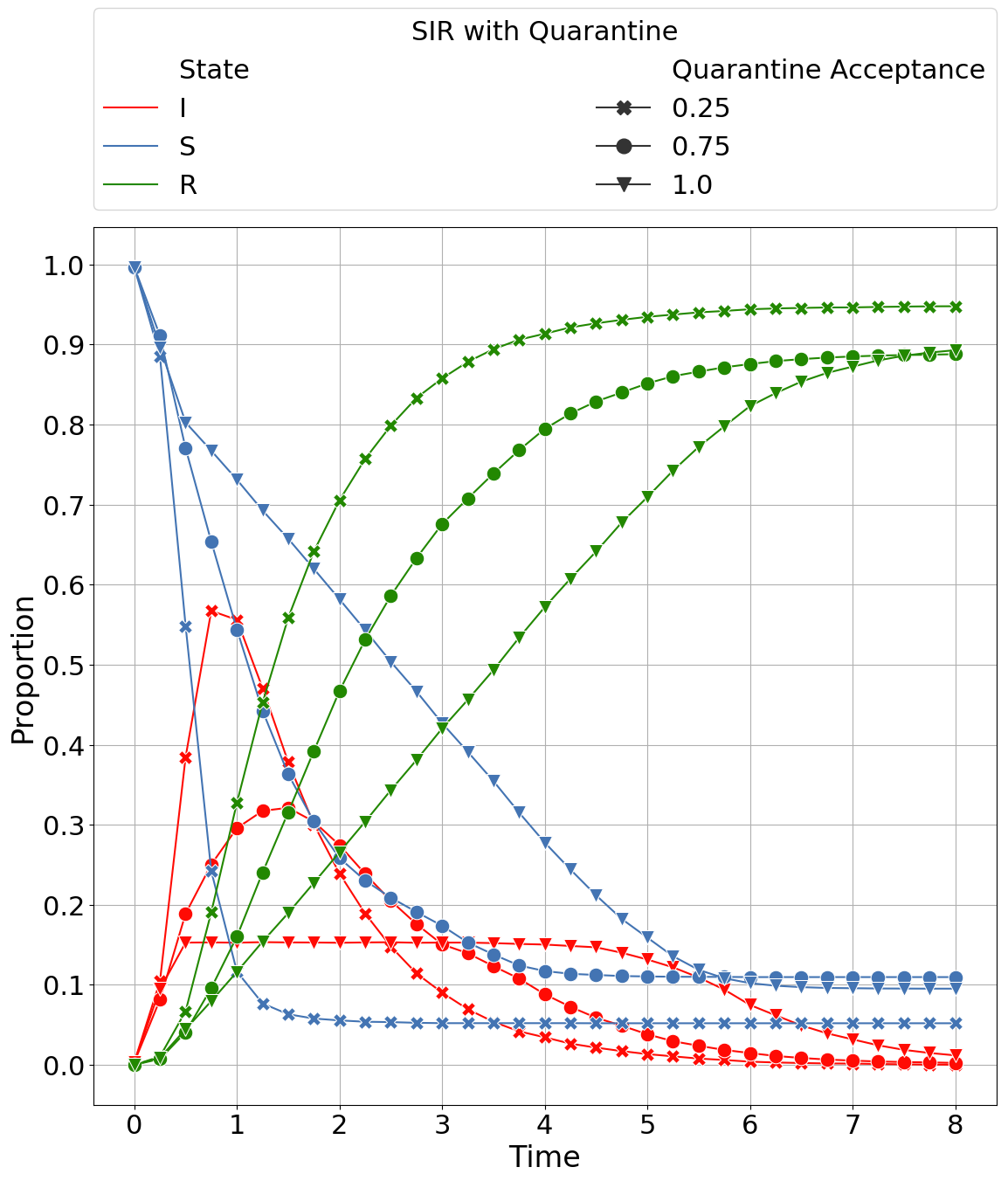
((b)) Quarantine Acceptance (QA) sweep. $QT=0.15,\gamma=1,\beta=3,\lambda=8$

Figure 7: Emergent behaviour for a SIR model with quarantines.

In this example multiple complex system’s features converge. We shall highlight how the combination of such features expand the modelling capabilities.

The utilisation of explicit and dynamic structures, together with the modelling of weak emergence, allowed for the description of complex infection dynamics over evolving networks. This allows for modelling the spread of an infection as a contact process using explicit links that causally affect models (agents) at a same spatio-temporal level. This can be seen in the SIR-CM model, where the contact network is revealed as the system evolves. The utilisation of the upward causation mechanism is key for the development of such network: the size-biased distribution is generated based on the observed micro-level information.

In this experiment we stepped away from analysing the network structure impact over the epidemics. This analysis can be found in Newman et al. (2001); Pastor-Satorras et al. (2015); Ferreyra et al. (2021).

In regard of the social isolation model, the downward information mechanism closes the micro-macro level loop presenting strong emergence properties that are observed in Figure 7. These macro-level structures are a consequence of the micro-macro level interactions.

4 Discussion

By visiting different types of models for varied social systems we saw how archetypal structural features (see Table 1) can be modelled and implemented with EB-DEVS, and their relation with emergent properties.

In the Dissemination of Culture model, by means of the Fads and Fashion extension, we showed that introducing emergent properties (which impact noticeably the model’s phase transitions) can be done in a compact and straightforward way, with minimal additions to a reference baseline model. In the example, we add strong emergence by including a simple rule that modifies the agents’ adaptive dynamics.

Afterwards, in the Segregation model we used an implicit communication structure, relying on the upward causation mechanism, to implement the agents’ coordination. This pattern allowed us to introduce weak emergence and stigmergy in the model.

Later on, in the Preferential Attachment and SIR models, we showed how evolving networks can produce complex behaviours. These behaviours are easily expressed with simple rules in EB-DEVS based on the state of macro-level variables.

Finally, with the Sugarscape model we showed how different types of models at the microscopic level can be integrated using implicit communication mechanisms. This is, we established a well-defined separation of concerns between atomic models of type Cell and Agent, and defined their rules of interaction by means of algorithms at the global transition function. Furthermore, the addition of strong emergent behaviour allowed for the definition of macro-level variables that influence back the behaviour of micro-level models.

Considering the implemented models, we highlight the following salient aspects:

• EB-DEVS helps the modeller to deal with systems requiring a multilevel treatment by relying on a well-defined multilevel framework featuring unambiguous simulation rules. This avoids the development of ad hoc single-use mechanisms to resolve the interaction between the micro and macroscopic levels.

• The decision to resort to closed micro-macro feedback loops or to use only partial micro-macro communication (upstream or downstream) can be made at any point in the modelling process with minimal impact on the previously modelled dynamics.

• Evolving from models without emergent behaviour to extensions that include some form of emergence is a straightforward task that preserves the structure of the base model, thus facilitating also the assessment of the impact of emergence processes compared to more simplified versions of a same system model.

• Implicit and explicit communication structures can be easily integrated together to design elaborated coordination mechanisms. These communication patterns are often very useful while designing complex systems with adaptive agents.

• Dynamic communication structures (i.e., those that evolve with time) span evolving networks that are often seen in natural, social and engineered systems. In ABMs these structures require a higher level entity to manage the connections. This can be naturally modelled with EB-DEVS via the macro-level state.

5 Conclusions

In this paper we presented several classical models in computational sociology and implemented them with the EB-DEVS formalism. The chosen models are often considered as typical examples of complex systems and can exhibit various forms of emergent behaviour.

Throughout these case studies we have identified certain structural features by which the systems under study can be typified, and we show the relationship of these features to the activity of modelling emergent behaviour with EB-DEVS.

We showed different modelling practices that facilitated the modelling of explicit and implicit communication structures, static or dynamic, with or without micro-macro interaction, and with weak or strong emergent behaviour (in the latter case, accepting the live identification of the emergent property). In each example we discussed the role of communication structures in the development of multilevel simulation models, and illustrated how micro-macro feedback loops enable the modelling of macro-level properties.

Complex systems modelling is a necessary tool to explore and understand social processes by means of computer simulation, and it benefits from having formal mechanisms that allow global-level properties derived from local-level interactions. In this paper we showed how EB-DEVS permits conceptualising the analysed societies by incorporating emergent behaviour when required, for example by incorporating the concept of Gini in the Sugarscape model, Fads and Fashion in the Dissemination of Culture model or Quarantines in a SIR epidemic model.

However, although EB-DEVS has proven to be a convenient formalism for a wide variety of complex systems, further experimentation is needed. It remains necessary to demonstrate that the approach works as expected in multi-layered systems where micro-macro information traverses the system hierarchy across more than 2 levels (a feature common to all models exercised in this work). In addition, we have not yet explored the impact on simulation performance, which can be a key decision factor when selecting a M&S technology (especially for complex systems that are often composed of a large number of elements at the microscopic level).

References

- Epstein [2008] Joshua M. Epstein. Why Model? Journal of Artificial Societies and Social Simulation, 11(4), 10 2008. URL https://EconPapers.repec.org/RePEc:jas:jasssj:2008-57-1.
- Axelrod [1997] Robert Axelrod. The dissemination of culture: A model with local convergence and global polarization. Journal of Conflict Resolution, 1997. ISSN 00220027. doi:10.1177/0022002797041002001.
- Schelling [1971] Thomas C. Schelling. Dynamic models of segregation. The Journal of Mathematical Sociology, 1(2):143–186, 1971. ISSN 15455874. doi:10.1080/0022250X.1971.9989794.
- Tesfatsion [2002] Leigh Tesfatsion. Agent-based computational economics: growing economies from the bottom up., 2002. ISSN 10645462.
- Macy and Willer [2002] Michael W. Macy and Robert Willer. From factors to actors: Computational sociology and agent-based modeling, 2002. ISSN 03600572.
- Kermack and McKendrick [1927] W. O. Kermack and A. G. McKendrick. A Contribution to the Mathematical Theory of Epidemics. Proceedings of the Royal Society A: Mathematical, Physical and Engineering Sciences, 1927. ISSN 1364-5021. doi:10.1098/rspa.1927.0118.
- Edmonds and Hales [2005] Bruce Edmonds and David Hales. Computational simulation as theoretical experiment, 7 2005. ISSN 0022250X. URL https://www.tandfonline.com/doi/abs/10.1080/00222500590921283.
- Sawyer [2005] R. Keith Sawyer. Social emergence: Societies as complex systems. 2005. doi:10.1017/CBO9780511734892.
- Foguelman et al. [2021] Daniel Foguelman, Philipp Henning, Adelinde Uhrmacher, and Rodrigo Castro. EB-DEVS: A formal framework for modeling and simulation of emergent behavior in dynamic complex systems. Journal of Computational Science, 53:101387, jul 2021. doi:10.1016/j.jocs.2021.101387. URL https://doi.org/10.1016%2Fj.jocs.2021.101387.
- Zeigler et al. [2018] Bernard Zeigler, Alexandre Muzy, and Ernesto Kofman. Theory of modeling and simulation: Discrete event & iterative system computational foundations. Academic press, 2018. ISBN 0128133708.
- Mittal [2013] Saurabh Mittal. Emergence in stigmergic and complex adaptive systems: A formal discrete event systems perspective. Cognitive Systems Research, 21:22–39, 2013. ISSN 13890417. doi:10.1016/j.cogsys.2012.06.003.
- Szabo and Birdsey [2017] Claudia Szabo and Lachlan Birdsey. Validating Emergent Behavior in Complex Systems. In Advances in Modeling and Simulation, pages 47–62. Springer, 2017. doi:10.1007/978-3-319-64182-9_4.
- Vangheluwe [2000] H. L. M. Vangheluwe. DEVS as a common denominator for multi-formalism hybrid systems modelling. In CACSD. Conference Proceedings. IEEE International Symposium on Computer-Aided Control System Design (Cat. No.00TH8537), pages 129–134, 2000. doi:10.1109/cacsd.2000.900199.
- Zeigler [1976] Bernard Zeigler. Theory of modeling and simulation. John Wiley & Sons. Inc., New York, NY, 1976.
- Wainer and Giambiasi [2002] Gabriel Wainer and Norbert Giambiasi. N-dimensional Cell-DEVS models. Discrete Event Dynamic Systems: Theory and Applications, 12(2):135–157, 2002. ISSN 09246703. doi:10.1023/A:1014536803451.
- Chow and Zeigler [1994] Alex Chung Hen Chow and Bernard Zeigler. Parallel DEVS: a parallel, hierarchical, modular modeling formalism. In Winter Simulation Conference Proceedings, 1994. doi:10.1109/wsc.1994.717419.
- Barros [1997] Fernando J. Barros. Modeling formalisms for dynamic structure systems. ACM Transactions on Modeling and Computer Simulation, 7(4):501–515, 1997. ISSN 10493301. doi:10.1145/268403.268423.
- Uhrmacher [2001] A. M. Uhrmacher. Dynamic structures in modeling and simulation: A reflective approach. ACM Trans. Model. Comput. Simul., 11(2):206–232, April 2001. ISSN 1049-3301. doi:10.1145/384169.384173. URL https://doi.org/10.1145/384169.384173.
- Steiniger and Uhrmacher [2016] Alexander Steiniger and Adelinde M. Uhrmacher. Intensional Couplings in Variable-Structure Models. ACM Transactions on Modeling and Computer Simulation, 26(2):1–27, 2016. ISSN 10493301. doi:10.1145/2818641.
- Grassé [1959] Plerre-P Grassé. La reconstruction du nid et les coordinations interindividuelles chezBellicositermes natalensis etCubitermes sp. la théorie de la stigmergie: Essai d’interprétation du comportement des termites constructeurs. Insectes sociaux, 6(1):41–80, 1959.
- Tummolini et al. [2009] Luca Tummolini, Marco Mirolli, and Cristiano Castelfranchi. Stigmergic cues and their uses in coordination: An evolutionary approach. Agents, Simulation and Applications, pages 243–265, 2009.
- Wainer [2009] Gabriel Wainer. Discrete-event modeling and simulation: A practitioner’s approach. Second edition, 2009. ISBN 9781420053371. doi:10.1201/9781420053371.
- Campbell [1974] Donald T Campbell. ‘Downward causation’in hierarchically organised biological systems. In Studies in the Philosophy of Biology, pages 179–186. Springer, 1974. doi:10.1007/978-1-349-01892-5_11.
- Emmeche et al. [1997] Claus Emmeche, Simo Køppe, and Frederik Stjernfelt. Explaining Emergence: Towards an Ontology of Levels. Journal for General Philosophy of Science, 28(1):83–117, 1997. ISSN 09254560. doi:10.1023/A:1008216127933.
- Mittal and Rainey [2015] Saurabh Mittal and Larry Rainey. Harnessing emergence: The control and design of emergent behavior in system of systems engineering. In Proceedings of the conference on summer computer simulation, pages 1–10, 2015.
- Centola et al. [2007] Damon Centola, Juan Carlos Gonzlez-Avella, Víctor M. Eguíluz, and Maxi San Miguel. Homophily, cultural drift, and the co-evolution of cultural groups. Journal of Conflict Resolution, 51(6), 2007. ISSN 00220027. doi:10.1177/0022002707307632.
- Castellano et al. [2000] Claudio Castellano, Matteo Marsili, and Alessandro Vespignani. Nonequilibrium phase transition in a model for social influence. Physical Review Letters, 85(16), 2000. ISSN 00319007. doi:10.1103/PhysRevLett.85.3536.
- Balenzuela et al. [2015] Pablo Balenzuela, Juan Pablo Pinasco, and Viktoriya Semeshenko. The undecided have the key: Interaction-driven opinion dynamics in a three state model. PLoS ONE, 10(10), 2015. ISSN 19326203. doi:10.1371/journal.pone.0139572.
- Klemm [2003] Konstantin Klemm. Global Culture: A Noise Induced Transition in Finite Systems. 2003. doi:10.1063/1.1571335.
- Epstein [1999] Joshua M. Epstein. Agent-based computational models and generative social science. Complexity, 4(5):41–60, 1999. ISSN 10990526. doi:10.1002/(SICI)1099-0526(199905/06)4:5<41::AID-CPLX9>3.0.CO;2-F.
- Albert and Barabási [2002] Réka Albert and Albert László Barabási. Statistical mechanics of complex networks. Reviews of Modern Physics, 74(1), 2002. ISSN 00346861. doi:10.1103/RevModPhys.74.47.
- Epstein and Axtell [2018] Joshua M. Epstein and Robert L. Axtell. Growing Artificial Societies. 2018. doi:10.7551/mitpress/3374.001.0001.
- Dijkstra [1982] Edsger W. Dijkstra. On the Role of Scientific Thought. In Selected Writings on Computing: A personal Perspective. 1982. doi:10.1007/978-1-4612-5695-3_12.
- Mitzenmacher and Upfal [2005] M. Mitzenmacher and E. Upfal. Probability and computing: Randomized algorithms and probabilistic analysis. 2005.
- Bollobás [1998] Béla Bollobás. Random graphs. In Modern graph theory, pages 215–252. Springer, 1998.
- Decreusefond et al. [2012] Laurent Decreusefond, Jean-Stéphane Dhersin, Pascal Moyal, Viet Chi Tran, et al. Large graph limit for an sir process in random network with heterogeneous connectivity. The Annals of Applied Probability, 22(2):541–575, 2012.
- Volz [2008] Erik Volz. SIR dynamics in random networks with heterogeneous connectivity. Journal of Mathematical Biology, 56(3):293–310, 2008.
- Bocharov et al. [2011] P. P. Bocharov, C. D’Apice, and A. V. Pechinkin. Queueing Theory. 2011. doi:10.1515/9783110936025.
- Newman et al. [2001] M. E. J. Newman, S. H. Strogatz, and D. J. Watts. Random graphs with arbitrary degree distributions and their applications. Phys. Rev. E, 64:026118, Jul 2001. doi:10.1103/PhysRevE.64.026118. URL https://link.aps.org/doi/10.1103/PhysRevE.64.026118.
- Pastor-Satorras et al. [2015] Romualdo Pastor-Satorras, Claudio Castellano, Piet Van Mieghem, and Alessandro Vespignani. Epidemic processes in complex networks. Rev. Mod. Phys., 87:925–979, Aug 2015. doi:10.1103/RevModPhys.87.925. URL https://link.aps.org/doi/10.1103/RevModPhys.87.925.
- Ferreyra et al. [2021] Emanuel Javier Ferreyra, Matthieu Jonckheere, and Juan Pablo Pinasco. Sir dynamics with vaccination in a large configuration model. Applied Mathematics & Optimization, pages 1–50, 2021.