Online False Discovery Rate Control for LORD & SAFFRON Under Positive, Local Dependence

Abstract

Online testing procedures assume that hypotheses are observed in sequence, and allow the significance thresholds for upcoming tests to depend on the test statistics observed so far. Some of the most popular online methods include alpha investing, LORD++ (hereafter, LORD), and SAFFRON. These three methods have been shown to provide online control of the “modified” false discovery rate (mFDR) under a condition known as conditional superuniformity. However, to our knowledge, LORD & SAFFRON have only been shown to control the traditional false discovery rate (FDR) under an independence condition on the test statistics. Our work bolsters these results by showing that SAFFRON and LORD additionally ensure online control of the FDR under a “local” form of nonnegative dependence. Further, FDR control is maintained under certain types of adaptive stopping rules, such as stopping after a certain number of rejections have been observed. Because alpha investing can be recovered as a special case of the SAFFRON framework, our results immediately apply to alpha investing as well. In the process of deriving these results, we also formally characterize how the conditional superuniformity assumption implicitly limits the allowed p-value dependencies. This implicit limitation is important not only to our proposed FDR result, but also to many existing mFDR results.

1 INTRODUCTION

In traditional, prespecified hypothesis testing, all hypotheses are known before the experiment begins. A typical goal is to limit the probability of any false discoveries (the familywise error rate, or FWER; see, for example Efron and Hastie,, 2016) to be no less than a constant denoted by $\alpha$ (e.g., $\alpha=0.05$). One simple method for FWER control is to “budget” or “spend” a predefined fraction of the allowed FWER on each planned test, so that the sum of thresholds used across all tests is equal to $\alpha$.

In contrast, online testing procedures assume that researchers observe a (possibly infinite) sequence of hypotheses and associated test statistics. Because the number of hypotheses is unknown in advance, budgeting the alpha level across all hypotheses is not always feasible. Instead, in a landmark paper, Foster and Stine, (2008) propose a method known as alpha-investing in which rejection thresholds for future tests are determined as a function of the statistics observed so far. Under this framework, each rejected hypothesis replenishes the available alpha budget, or “alpha wealth,” allowing users to continue testing indefinitely.

Alpha-investing formed the inspiration for a wave of new online methods. Aharoni and Rosset, (2014) extend this idea to “generalized” alpha-investing (GAI), and Ramdas et al., (2017) propose a version of GAI with improved power (GAI++). The latter class of methods includes a special case known as LORD++ (significance Levels based On Recent Discovery; hereafter referred to as LORD), which is based on a method developed by Javanmard and Montanari, (2018). Building on LORD, Ramdas et al., (2018) develop a similar method that incorporates adaptive estimates of the proportion of true null hypotheses, referred to as “SAFFRON” (Serial estimate of the Alpha Fraction that is Futilely Rationed On true Null hypotheses).

Due to their relatively high power, LORD and SAFFRON are often described as being among the state-of-the-art methods available for online testing (Chen and Kasiviswanathan,, 2020; Zhang et al.,, 2020). The concepts underlying these two methods have also influenced several related online approaches (Tian and Ramdas,, 2019; Zrnic et al.,, 2020, 2021; Xu and Ramdas,, 2020; Weinstein and Ramdas,, 2020). Moreover, Ramdas et al., (2018) show that SAFFRON encompasses the original alpha investing method as a special case.

Existing theoretical studies of alpha investing, LORD, and SAFFRON typically require a condition known as conditional superuniformity (CS), which states that each null p-value is statistically larger than a uniform random variable, conditional on the information used to specify its rejection threshold (Zrnic et al.,, 2021; see also Foster and Stine,; Ramdas et al.,; Ramdas et al.,). Thus, each p-value in the sequence may be “locally dependent” with its neighbors, so long as its associated rejection threshold is specified sufficiently far in advance (see details in Section 2.2, below). For example, if when several hypotheses are tested on each of several subpopulations, then the resulting p-value sequence can be said to follow local dependence, as tests conducted in one population are independent of tests conducted in another. Similarly, local dependence holds approximately if the test statistics are associated with a temporal process with an autoregressive correlation structure.

Under the CS assumption, LORD, and SAFFRON have been shown to control a “modified” version of the false discovery rate (mFDR) (Ramdas et al.,, 2017, 2018; Zrnic et al.,, 2021). To our knowledge however, existing results for online control of the traditional false discovery rate (FDR; Benjamini and Hochberg,, 1995) require an additional assumption of p-value independence (Ramdas et al.,, 2017, 2018; Zrnic et al.,, 2021).

Our primary contribution is to show that LORD and SAFFRON also ensure online control of the FDR under a positive, local dependency condition on the p-values. In particular, they control FDR whenever (1) the null p-values are CS given the information used to define their testing thresholds (as in Zrnic et al.,, 2021); (2) the null p-values follow the conventional assumption of positive regression dependence on a subset (Benjamini and Yekutieli,, 2001), and (3) users choose significance thresholds that are monotonically nonincreasing in the p-values that have been observed so far. Because alpha investing can be written as a special case, the same results immediately apply to alpha investing as well.

As a secondary contributions, we show that FDR control is also possible under weakened forms of monotonicity, which allows us to account for certain forms of adaptive stopping times. We also illustrate convenient, special cases of the LORD and SAFFRON algorithms that may facilitate their communication and implementation. Our proposed variations offer added flexibility in scenarios where the logistics of hypothesis ordering are beyond the analyst’s control.

Finally, we introduce an important caveat regarding the CS assumption, which is relevant to many results in the literature beyond our own. For well-powered p-value sequences, we show that CS can only be satisfied under local dependence. To our knowledge, this is the first formal characterization of CS as a dependence requirement.

The remainder of this paper is organized as follows. In Section 2, we introduce relevant notation, summarize LORD and SAFFRON, and present existing results for FDR control. In the process, we introduce the CS assumption and show how it implicitly restricts p-value dependencies. Section 3 contains our main result, and discusses variations on the required positive dependence and monotonicity conditions. Section 4 outlines convenient, special cases of the LORD and SAFFRON algorithms. Section 5 illustrates our main result in a series of simulations. All proofs are contained in the supplementary materials.

2 NOTATION & PRELIMINARIES

Following Foster and Stine, (2008), we consider the setting where analysts observe a (possibly infinite) sequence of hypotheses $\{H_{1},H_{2},\dots\}$, along with corresponding p-values $\{P_{1},P_{2},\dots\}$. Let $\mathcal{H}_{0}\subseteq\mathbb{N}$ be the subset of indices corresponding to the truly null hypotheses. At each stage $t$ of testing, the researcher observes $P_{t}$ and must decide to reject or not reject $H_{t}$ before observing the next test statistic $P_{t+1}$.

Let $\alpha_{t}$ be the significance threshold used for testing $H_{t}$, where $H_{t}$ is rejected whenever $P_{t}\leq\alpha_{t}$. In order to capture different types of adaptive decision making, Foster and Stine, (2008) allow $\alpha_{t}$ to be a function of the preceding p-values $\{P_{i}\}_{i<t}$. To highlight that $\alpha_{t}$ may only depend on some summary function of $\{P_{i}\}_{i<t}$, we use $\mathcal{F}_{t-1}$ to denote the minimal set of real-valued random variables needed to determine the threshold $\alpha_{t}$. For example, if a decision rule defines $\alpha_{t}$ only as a function of which hypotheses have been rejected so far, then $\mathcal{F}_{t-1}=\{1(P_{i}<\alpha_{i})\}_{i<t}$. In this framing, an online testing method is essentially a set of rules for translating previous p-values into thresholds for the future tests. Each threshold $\alpha_{t}$ is a random variable, but must be fully determined given $\mathcal{F}_{t-1}$.

Let $\mathcal{R}_{t}=\{i\leq t:P_{i}\leq\alpha_{i}\}$ be indices for the hypothesis that are rejected by the $t^{th}$ stage of testing. At each stage $t$, the false discovery proportion (FDP) and the false discovery rate (FDR) are defined respectively as

$$\text{FDP}(t)=\frac{|\mathcal{H}_{0}\cap\mathcal{R}_{k}|}{1\vee|\mathcal{R}_{k}|}\hskip 6.99997pt\text{and}\hskip 6.99997pt\text{FDR}(t)=\mathbb{E}\left[\frac{|\mathcal{H}_{0}\cap\mathcal{R}_{k}|}{1\vee|\mathcal{R}_{k}|}\right],$$

where $(a\vee b)$ is shorthand for the maximum over $\{a,b\}$. Similarly, the “modified” FDR is defined as

$$\text{mFDR}(t)=\frac{\mathbb{E}\left[|\mathcal{H}_{0}\cap\mathcal{R}_{k}|\right]}{\mathbb{E}\left[1\vee|\mathcal{R}_{k}|\right]}.$$

2.1 LORD & SAFFRON Approaches

Ramdas et al., (2017) suggest choosing the thresholds $\{\alpha_{i}\}_{i=1}^{\infty}$ in a way that ensures that an empirical estimate of the false discovery proportion never exceeds $\alpha$. The authors estimate the FDP as

$$\widehat{\text{FDP}}_{0}(t)=\frac{\sum_{i\leq t}\alpha_{i}}{1\vee|\mathcal{R}_{t}|},$$

and propose a specific algorithm (LORD) for defining thresholds $\{\alpha_{t}\}_{t=1}^{\infty}$ so that $\widehat{\text{FDR}}_{0}(t)\leq\alpha$ for all $t\in\mathbb{N}$. A key attribute of LORD is that it is a monotonic algorithm, meaning that rejecting more p-values early on can only lead to higher testing thresholds later on (see Theorem 2 for a formal definition). Thus, observing a stronger signal in early tests can only improve power for later tests. We defer the full details of the LORD algorithm to the supplemental materials, and present a simplified, special case of the algorithm in Section 4.

Intuitively, we may expect that constraining $\widehat{\text{FDR}}_{0}(t)\leq\alpha$ will result in a small false discovery proportion, since

$$\widehat{\text{FDP}}_{0}(t) \geq\frac{\sum_{\{i\leq t:i\in\mathcal{H}_{0}\}}\alpha_{i}}{1\vee|\mathcal{R}_{t}|}$$ (1)

$$\approx\frac{\sum_{\{i\leq t:i\in\mathcal{H}_{0}\}}\mathbf{1}(P_{i}\leq\alpha_{i})}{1\vee|\mathcal{R}_{t}|}$$

$$=\text{FDP}(t).$$

Thus, $\widehat{\text{FDP}}_{0}(t)$ is an approximate overestimate of $\text{FDP}(t)$, and so we can intuit that controlling $\widehat{\text{FDP}}_{0}(t)$ will result in conservative control for $\text{FDR}(t)$. Indeed, Ramdas et al., (2017) show that, under certain conditions, LORD guarantees both $\text{mFDR}(t)\leq\alpha$ and $\text{FDR}(t)\leq\alpha$ for all $t\in\mathbb{N}$. Importantly, these results apply not only to the specific LORD algorithm, but to any monotonic algorithm satisfying $\widehat{\text{FDP}}_{0}(t)\leq\alpha$ for all $t$ (see details in Theorem 2, below). Since $\widehat{\text{FDP}}_{0}(t)$ is directly observable, the requirement that $\widehat{\text{FDP}}_{0}(t)\leq\alpha$ is straightforward to implement.

Building on this idea, Ramdas et al., (2018) suggest controlling an alternative estimate of $\text{FDP}(t)$ that is expected to be less conservative. Leveraging strategies from Storey, (2002) and Storey et al., (2004), Ramdas et al., propose the estimator

$$\widehat{\text{FDP}}_{\mathbf{\lambda}}(t)=\frac{\sum_{i\leq t}\alpha_{i}\frac{\mathbf{1}(P_{i}>\lambda_{i})}{1-\lambda_{i}}}{1\vee|\mathcal{R}_{t}|},$$ (2)

where $\{\lambda_{i}\}_{i=1}^{\infty}$ is a series of user-defined constants within the interval $(0,1)$. Like $\alpha_{i}$, each $\lambda_{i}$ is required to be a deterministic function of $\mathcal{F}_{i-1}$. The intuition of $\widehat{\text{FDP}}_{\mathbf{\lambda}}(t)$ is that $\mathbf{1}(P_{i}>\lambda_{i})/(1-\lambda_{i})$ has expectation lower bounded by 1 when $i\in\mathcal{H}_{0}$, but has a smaller expectation when $i\notin\mathcal{H}_{0}$. Thus, the numerator in Eq (2) will ideally have an expectation close to $\sum_{\{i\leq t:i\in\mathcal{H}_{0}\}}\alpha_{i}$, and so $\widehat{\text{FDP}}_{\mathbf{\lambda}}(t)$ will ideally resemble right-hand side of Line (1). In simulations, Ramdas et al., generally found setting $\lambda=1/2$ to produce algorithms with relatively high power.

Ramdas et al., develop a monotonic algorithm known as SAFFRON that assigns threshold parameters $\{\alpha_{i}\}_{i=1}^{\infty}$ and tuning parameters $\{\lambda_{i}\}_{i=1}^{\infty}$ such that $\widehat{\text{FDP}}_{\mathbf{\lambda}}(t)$ is constrained to be no more than $\alpha$ at all stages $t\in\mathbb{N}$. Again, we defer the full details of this algorithm to the supplemental materials, and illustrate a simplified, special case in Section 4. Ramdas et al., show that, under certain conditions, any monotonic algorithm satisfying $\widehat{\text{FDP}}_{\mathbf{\lambda}}(t)\leq\alpha$ for all $t\in\mathbb{N}$ (including SAFFRON) controls mFDR and FDR. We review the required conditions in the next two sections.

2.2 Conditional Superuniformity

Next, we study the conditional superuniformity (CS) assumption, which forms the basis for many procedures in the online testing field. Formally, we say that a p-value $P_{t}$ satisfies CS if $\mathbb{P}(P_{t}\leq u|\mathcal{F}_{t-1})\leq u$, i.e., $P_{t}$ is a valid p-value even conditional on the information used to define its rejection threshold, $\mathcal{F}_{t-1}$. This assumption is nontrivial to verify: if joint distribution of underlying test statistics is completely unknown, then there is no clear way to produce p-values that are CS.

Zrnic et al., (2021) propose a clever means of circumventing this problem when partial knowledge of this joint distribution is available. In particular, the authors consider cases where each p-value is dependent only with a subset of its neighbors. Reflecting these local relationships, we will refer to a p-value $P_{t}$ as following local dependence whenever $P_{t}$ is independent of the information ($\mathcal{F}_{t-1}$) used to define its thresholds $(\alpha_{t},\lambda_{t})$.f For example, suppose that test statistics are observed in batches, and are known to be independent across batches. Let $b_{t}$ be the batch label for the $t^{th}$ hypothesis. Even if the within-batch dependencies are unknown, we can still proceed by choosing parameters for upcoming tests only based on the test statistics from previous batches. By constraining $\mathcal{F}_{t-1}$ to be a function of $\{P_{i}:b_{i}<b_{t}\}$, we can effectively ignore the within-batch dependencies, as $\mathbb{P}(P_{t}\leq\alpha_{t}|\mathcal{F}_{t-1})=\mathbb{P}(P_{t}\leq\alpha_{t})$.

While CS is often implied by local dependence, it is not immediately obvious whether the reverse is true. A more precise understanding of how CS restricts dependencies does not appear to have been illustrated in the literature. To explore this link further, we propose the following, novel remark.

Remark 1.

(CS Necessary Conditions)If $P_{t}$ is continuous, then $P_{t}$ can satisfy CS only if one of the following two conditions holds.

1. ($P_{t}$ follows locally dependence) $P_{t}\perp\mathcal{F}_{t-1}$.

2. ($P_{t}$ is underpowered) There exists an alternative p-value $P_{t}^{\prime}$ satisfying both CS and local dependence, and that is strictly more powerful than $P_{t}$. More specifically, there exists a random variable $P_{t}^{\prime}$ satisfying $\mathbb{P}(P_{t}^{\prime}\leq u|\mathcal{F}_{t-1})=u$; $P_{t}^{\prime}\perp\mathcal{F}_{t-1}$; $P_{t}^{\prime}\leq P_{t}$; and $\mathbb{P}(P_{t}^{\prime}<P_{t})>0$.

The implication of the Remark 1 is that, in order to achieve CS, we must either plan testing thresholds for $P_{i}$ only using variables that are uninformative of $P_{i}$ (as in Zrnic et al.,, 2021), or we must use p-values that are underpowered. That is, for well-powered p-value sequences, local dependence is a necessary condition for CS.

2.3 Existing FDR Bounds for LORD and SAFFRON, Under Independence

Zrnic et al., (2021) show that LORD and SAFFRON each control mFDR under the CS condition (see their Theorem 2; as well as Ramdas et al.,, 2017; and Ramdas et al.,, 2018).

Theorem 1.

(mFDR under CS) Assume that all p-values satisfy CS (i.e., $\mathbb{P}(P_{t}\leq u|\mathcal{F}_{t-1})$ for all $t\in\mathbb{N}$), and that $\alpha_{t}$ and (when applicable) $\lambda_{t}$ are deterministic functions of $\mathcal{F}_{t-1}$. Under these conditions, the following two results hold.

1. (LORD mFDR Control) If the parameters $\{\alpha_{i}\}_{i\in\mathbb{N}}$ are selected so that $\widehat{\text{FDR}}_{0}(t)\leq\alpha$ for all $t\in\mathbb{N}$ (e.g., LORD) then $\text{mFDR}(t)\leq\alpha$.

2. (SAFFRON FDR Control) If the parameters $\{\alpha_{i},\lambda_{i}\}_{i\in\mathbb{N}}$ are selected so that $\widehat{\text{FDR}}_{\lambda}(t)\leq\alpha$ for all $t\in\mathbb{N}$ (e.g., SAFFRON) then $\text{mFDR}(t)\leq\alpha$.

Additionally, Ramdas et al., (2017) and Ramdas et al., (2018) show that traditional FDR control is achieved under a combination of CS, a monotonicity condition, and a p-value independence condition.

Theorem 2.

(FDR under independence) In addition to the conditions of Theorem 1, we make the following assumptions.

1. (Independence) The null p-values are independent of each other and the non-nulls;

2. (Monotonicity) For each $t\in\mathbb{N}$, the parameters $\alpha_{t}$ and (when applicable) $\lambda_{t}$ are deterministic, coordinatewise nondecreasing functions of the set of indicators $\mathcal{F}_{t-1}:=(\mathbf{1}(P_{1}\leq\alpha_{1}),\dots,\mathbf{1}(P_{t-1}\leq\alpha_{t-1}),\mathbf{1}(P_{1}\leq\lambda_{1}),\dots,\mathbf{1}(P_{t-1}\leq\lambda_{t-1}))$. Note that, for LORD, this condition can be simplified by fixing each $\lambda_{t}=0$.

Under the above conditions, the following two results hold.

1. (LORD FDR Control) If the parameters $\{\alpha_{i}\}_{i\in\mathbb{N}}$ are selected so that $\widehat{\text{FDR}}_{0}(t)\leq\alpha$ for all $t\in\mathbb{N}$ (e.g., LORD) then $\text{FDR}(t)\leq\alpha$.

2. (SAFFRON FDR Control) If the parameters $\{\alpha_{i},\lambda_{i}\}_{i\in\mathbb{N}}$ are selected so that $\widehat{\text{FDR}}_{\lambda}(t)\leq\alpha$ for all $t\in\mathbb{N}$ (e.g., SAFFRON) then $\text{FDR}(t)\leq\alpha$.

The monotonicity condition in Theorem 2 essentially states that lower p-values never lead us to require stricter thresholds in future tests – the more hypotheses we reject, the easier it will be to reject future hypotheses. This monotonicity condition can be ensured by design.

In the next section, we show that the additional assumptions made in Theorem 2 can be greatly relaxed. Most notably, the independence assumption can be weakened to a positive dependence assumption. That said, we still require conditional superuniformity.

3 FDR CONTROL UNDER POSITIVE DEPENDENCE

In Section 3.1, below, we introduce a monotonicity condition and a nonnegative dependence condition. We then present our main result, along with a sketch of the proof. In Sections 3.2, we discuss how certain forms of adaptive stopping rules can be formalized under our assumptions.

3.1 Main Result

Our first required condition for online FDR control is analogous to the monotonicity conditions described in Theorem 2, and can similarly be ensured by design. We will require that any decrease to a p-value (i.e., making it “more significant”) cannot decrease the total number of rejections.

Condition 1.

(Relaxed Monotonicity) For any $t\in\mathbb{N}$ and for any two p-value vectors $\mathbf{p}=(p_{1},\dots,p_{t})$ and $\mathbf{p}^{\prime}=(p_{1}^{\prime},\dots,p_{t}^{\prime})$ that could possibly result from the first $t$ tests, if $p_{i}\leq p_{i}^{\prime}$ for all $i\leq t$, then $\mathbf{p}$ must produce at least as many rejections as $\mathbf{p}^{\prime}$.

The most straightforward way to ensure Condition 1 is to require that each threshold $\alpha_{t}$ be a monotonic, nonincreasing function of the preceding p-values $(P_{1},\dots,P_{t-1})$. However, we will see in the next section that weaker versions of monotonicity can also satisfy Condition 1.

In order to relax the independence requirement in Theorem 2, we next introduce a version of the well-known positive regression dependence on a subset (PRDS) condition developed by Benjamini and Yekutieli, (2001). This condition will depend on the notion of increasing sets. A set of $k$-dimensional vectors $D\in[0,1]^{k}$ is called increasing if, for any vector $\mathbf{x}=(x_{1},\dots,x_{t})\in D$ and any vector $\mathbf{y}=(y_{1},\dots,y_{t})$ satisfying $x_{i}\leq y_{i}$ for all $i$, it must also be that $\mathbf{y}\in D$. For example, for any $r\leq t$, Condition 1 implies that the set of p-values that produce no more than $r$ rejections by stage $t$ is an increasing set.

Condition 2.

(Conditional PRDS) For any stage $t$, any null index $i\leq t$ satisfying $i\in\mathcal{H}_{0}$, and increasing set $D\subset[0,1]^{t}$, the probability $\mathbb{P}((P_{1},\dots,P_{t})\in D|P_{i}=u,\mathcal{F}_{i-1})$ is nondecreasing in $u$.

Roughly speaking Condition 2 says that each null p-value is positively associated with the other p-values. As with local dependence, we may expect Condition 2 to hold when sequentially analyzing population subgroups, with several hypotheses tested per group. We may also expect Condition 2 to hold when studying temporal test statistics believed to follow an autoregressive structure.

The key take-away from Conditions 1 & 2 is that, together, they imply that low p-values in early stages of the sequence tend to be associated with a higher number of rejections by later stages of the sequence. This idea will play a central role in our derivation of FDR control.

Theorem 3.

(FDR under nonnegative dependence) Under Conditions 1 & 2, if the p-values are conditionally superuniform (i.e., $\mathbb{P}(P_{t}\leq u|\mathcal{F}_{t-1})\leq u)$ for all $t\in\mathbb{N}$), then the following two results hold.

1. (LORD FDR Control) If the parameters $\{\alpha_{i}\}_{i\in\mathbb{N}}$ are selected so that $\widehat{\text{FDR}}_{0}(t)\leq\alpha$ for all $t\in\mathbb{N}$ (e.g., LORD) then $\text{FDR}(t)\leq\alpha$.

2. (SAFFRON FDR Control) If the parameters $\{\alpha_{i},\lambda_{i}\}_{i\in\mathbb{N}}$ are selected so that $\widehat{\text{FDR}}_{\lambda}(t)\leq\alpha$ for all $t\in\mathbb{N}$ (e.g., SAFFRON) then $\text{FDR}(t)\leq\alpha$.

Importantly, Theorem 3 still requires the CS condition. Thus, for well-powered p-value sequences, Theorem 3 effectively requires the p-values satisfy nonnegative, local dependence (see Section 2.2).

A sketch of the intuition for Theorem 3 is as follows. Consider the especially simple case where all parameters $\{\alpha_{i},\lambda_{i}\}_{i\in\mathbb{N}}$ are fixed a priori (i.e., $\mathcal{F}_{i-1}=\emptyset$ for all $i$). This setting greatly simplifies the notation needed, and still sheds light on how Theorem 3 can be proved when $\alpha_{i}$ and $\lambda_{i}$ are determined adaptively (see comments below). Under Conditions 1 & 2, smaller null p-values are generally associated with larger values for $(1\vee|\mathcal{R}_{t}|)$. Thus, for any $i\in\mathcal{H}_{0}$ and $t\geq i$, we would expect the rejection indicator $\mathbf{1}(P_{i}\leq\alpha_{i})$ to be negatively correlated with $1/(1\vee|\mathcal{R}_{t}|)$, i.e.,

$$\mathbb{E}\left[\frac{1}{1\vee|\mathcal{R}_{t}|}\mathbf{1}(P_{i}\leq\alpha_{i})\right]\leq\mathbb{E}\left[\frac{1}{1\vee|\mathcal{R}_{t}|}\right]\mathbb{E}\left[\mathbf{1}(P_{i}\leq\alpha_{i})\right].$$ (3)

Applying this, we have

$$\text{FDR}(t)= \sum_{\{i\leq t;i\in\mathcal{H}_{0}\}}\mathbb{E}\left[\frac{\mathbf{1}(P_{i}\leq\alpha_{i})}{1\vee|\mathcal{R}_{t}|}\right]$$

$$\leq \sum_{\{i\leq t;i\in\mathcal{H}_{0}\}}\mathbb{E}\left[\frac{1}{1\vee|\mathcal{R}_{t}|}\right]\mathbb{E}\left[\mathbf{1}(P_{i}\leq\alpha_{i})\right]$$

$$\leq \sum_{\{i\leq t;i\in\mathcal{H}_{0}\}}\mathbb{E}\left[\frac{1}{1\vee|\mathcal{R}_{t}|}\right]\alpha_{i}$$

$$= \mathbb{E}\left[\sum_{\{i\leq t;i\in\mathcal{H}_{0}\}}\frac{\alpha_{i}}{1\vee|\mathcal{R}_{t}|}\right],$$ (4)

where the first inequality comes from Eq (3), and the second inequality comes from $\mathbb{P}(P_{i}\leq\alpha_{i})=\mathbb{P}(P_{i}\leq\alpha_{i}|\mathcal{F}_{i-1})\leq\alpha_{i}$. Thus, if $\widehat{\text{FDP}}_{0}(t)=\sum_{i\leq t}\frac{\alpha_{i}}{|1\vee\mathcal{R}_{t}|}\leq\alpha$, then monotonicity of expectations implies that $\text{FDR}(t)\leq\alpha$.

To sketch the result for $\widehat{\text{FDP}}_{\lambda}$, we build on Eq (4) by multiplying each summation term by $\mathbb{E}\left[\mathbf{1}(P_{i}>\lambda_{i})\right]/(1-\lambda)\geq 1$. We obtain

$$\text{FDR}(t) \leq\sum_{\{i\leq t;i\in\mathcal{H}_{0}\}}\mathbb{E}\left[\frac{\alpha_{i}}{1\vee|\mathcal{R}_{t}|}\right]\frac{\mathbb{E}\left[\mathbf{1}(P_{i}>\lambda_{i})\right]}{1-\lambda_{i}}$$

$$\leq\sum_{\{i\leq t;i\in\mathcal{H}_{0}\}}\mathbb{E}\left[\frac{\alpha_{i}\frac{\left[\mathbf{1}(P_{i}>\lambda_{i})\right]}{1-\lambda_{i}}}{1\vee|\mathcal{R}_{t}|}\right],$$

where the second inequality comes from the fact that indicators of large p-values, $\mathbf{1}(P_{i}>\lambda_{i})$, are positively correlated with $\left(1\vee|\mathcal{R}_{t}|\right)^{-1}$. From here, if $\widehat{\text{FDP}}_{\lambda}(t)\leq\alpha$, then monotonicity of expectations again implies that $\text{FDR}(t)\leq\alpha$. In the full details of the proof, we also iterate expectations over $\mathcal{F}_{i-1}$ in order to account for adaptively defined parameters $\alpha_{i}$ and $\lambda_{i}$ (see the supplemental materials).

3.2 Incorporating Certain Forms of Adaptive Stopping Rules

While Theorem 3 ensures FDR control at fixed times $t\in\mathbb{N}$, it does not uniformly control the FDR across all times $t$. That is, we cannot conclude from Theorem 3 that $\sup_{t\in\mathbb{N}}\text{FDR}(t)\leq\alpha$. The practical relevance of this point is that some analysts may choose their final test stage adaptively, in the hopes rejecting a large proportion of the hypotheses tested. In other words, they may wish to stop testing early in the face of especially strong preliminary results. We show in this section that, for certain types of adaptive stopping rules, the conditions required for Theorem 3 still hold.

We will use $T$ to denote an adaptively determined stopping time, and will say that FDR is controlled under adaptive stopping times if $\mathbb{E}\left[\text{FDR}(T)\right]\leq\alpha.$ We will generally assume that $\mathbf{1}(T>t)$ is a deterministic function of $(P_{1},\dots,P_{t-1})$, and that $T$ is upper bounded (with probability 1) by a known constant $t_{\text{max}}$.

At first glance, it appears straightforward to account for these kinds of adaptive stopping times by simply setting $\alpha_{t}$ equal to zero for every stage $t>T$, and continuing testing until stage $t_{\text{max}}$. By controlling $\text{FDR}(t_{\text{max}})$, we effectively control $\mathbb{E}\left[\text{FDR}(T)\right]$. Unfortunately, such a method of assigning thresholds is not monotonic in the observed p-values. Seeing a sufficient number of rejections may cause us to lower our thresholds for all future tests by setting them to zero, and so the monotonicity conditions in Theorem 2 are not satisfied.

However, even though these kinds of stopping rules are not compatible with monotonicity constraints in Theorem 2, there are several types of adaptive stopping rules that still maintain Condition 1. In particular, Condition 1 may still be satisfied if users combine a monotone threshold function with a monotone stopping rule. To formalize these types of rules, let $\{\beta_{i}\}_{i=1}^{\infty}$ be a sequence of functions used for defining thresholds, where $\beta_{i}:[0,1]^{i-1}\rightarrow[0,1]$ is a mapping from first $i-1$ p-values to the threshold $\alpha_{i}=\beta_{i}(P_{1},\dots,P_{i-1})$.

As a first example, consider the case where users assign each threshold $\alpha_{i}$ according to a coordinatewise nonincreasing function $\beta_{i}^{\text{noninc}},$ but can also decide to stop testing if a certain critical threshold $\gamma^{\text{max-R}}$ of rejections have been made, or if a certain number of tests $\gamma^{\text{max-stage}}$ have completed. This implies the following form for each function $\beta_{i}$

$$\beta_{i}(P_{1},\dots,P_{i-1}) =\beta_{i}^{\text{noninc}}(P_{1},\dots,P_{i-1})$$

$$\hskip 10.00002pt\times\mathbf{1}\left(|\mathcal{R}_{i-1}|<\gamma^{\text{max-R}}\right)$$

$$\hskip 10.00002pt\times\mathbf{1}\left(i\leq\gamma^{\text{max-stage}}\right).$$

Here, the overall function $\beta_{i}$ is not monotonic – smaller p-values will increase future thresholds at first, but eventually will cause them to drop to zero. Still, even though the thresholds themselves are not monotonic in the p-value sequence, the total number of rejections is monotonic in the p-value sequence. Any decrease to a p-value can lead to a cease of testing, but cannot decrease the total number of rejections, and so Condition 1 still holds.

A similar result holds if we allow the maximum number of rejections, or the maximum number of stages, to be extended in the face of strong signal in the preliminary tests. To formalize this, we can instead assume that each function $\beta_{i}$ has the following structure.

$$\beta_{i}(P_{1},\dots,P_{i-1}) =\beta_{i}^{\text{noninc}}(P_{1},\dots,P_{i-1})$$

$$\hskip 10.00002pt\times\mathbf{1}\left(|\mathcal{R}_{i-1}|<\beta^{\text{max-R}}(P_{1},\dots,P_{i-1})\right)$$

$$\hskip 10.00002pt\times\mathbf{1}\left(i\leq\beta^{\text{max-stage}}(P_{1},\dots,P_{i-1}\right),$$

where $\beta_{i}^{\text{max-R}}:[0,1]^{i-1}\rightarrow\mathbb{N}$ and $\beta_{i}^{\text{max-stage}}:[0,1]^{i-1}\rightarrow\mathbb{N}$ are nonincreasing functions of $(P_{1},\dots,P_{i-1})$. Here, roughly speaking, larger p-values in the early stages must produce either stricter thresholds $($via $\beta_{i}^{\text{noninc}}$), a lower number of maximum stages (via $\beta_{i}^{\text{max-stage}})$, or a lower number of maximum rejections (via $\beta_{i}^{\text{max-R}})$. Any of these changes can only reduce the number of total discoveries. We again see that Condition 1 holds: the threshold functions $\beta_{i}$ are not themselves monotonic, but the number of discoveries is still nonincreasing in the observed p-values.

4 CONVENIENT IMPLEMENTATIONS OF LORD & SAFFRON

Both LORD & SAFFRON require the user to specify a threshold $\alpha_{1}$ for the first test statistic $P_{1}$, as well as a sequence of tuning parameters $\{\gamma_{i}\}_{i=1}^{\infty}$ summing to one. If users place more weight on the early terms of this sequence, then LORD and SAFFRON will allocate more alpha wealth to the early stages of testing, as well as to tests immediately following a discovery.

While the details of these two algorithms are fairly involved, we remark in this section that they can be greatly simplified whenever $\{\gamma_{i}\}_{i=1}^{\infty}$ is chosen to be a geometric series. To our knowledge, the convenient forms of the LORD and SAFFRON algorithms discussed below have not been illustrated before.

We also include simplified versions of the algorithms outlined by Zrnic et al., (2021), which are designed to account for various forms of partially unknown dependencies among the test statistics (see summary in Section 2.2). In doing so, we also relax one of the “monotonicity” assumptions made by Zrnic et al.,.

4.1 Base implementations

We define $\pi\in[0,1]$ to be a user-specified constant representing the proportion of the available “alpha wealth” to be allocated to the current test. We show in the supplemental materials that, if we choose tuning parameters $\alpha_{1}=\pi\alpha$ and $\gamma_{i}=\pi(1-\pi)^{i-1}$ for $i\in\mathbb{N}$, then the LORD algorithm becomes equivalent to setting

$$\alpha_{t}=\left\{\alpha\left(1\vee|\mathcal{R}_{t-1}|\right)-\sum_{i\leq t-1}\alpha_{i}\right\}\pi$$ (5)

for all $t\in\mathbb{N}$, where $\mathcal{R}_{0}=\emptyset$. It is readily apparent that defining $\alpha_{t}$ in this way ensures that $\widehat{\text{FDR}}_{0}(t)\leq\alpha$ for all $t\in\mathbb{N}$.

The SAFFRON algorithm described by Ramdas et al., (2018) additionally requires users to specify a constant $\lambda\in(0,1)$, and sets $\lambda_{i}=\lambda$ for all $i\in\mathbb{N}.$ Under the same choice of tuning parameters as above (see details in the supplemental materials), SAFFRON similarly reduces to setting setting each $\alpha_{t}=\min\{\lambda_{t},\bar{\alpha}_{t}\}$, where

$$\bar{\alpha}_{t} =\left\{\alpha\left(1\vee|\mathcal{R}_{t-1}|\right)-\sum_{i\leq t-1}\frac{\bar{\alpha}_{i}\mathbf{1}(P_{i}>\lambda)}{1-\lambda}\right\}\left(1-\lambda\right)\pi.$$ (6)

By rearranging terms, we can see that this choice of $\{\lambda_{t},\alpha_{t}\}_{t=1}^{\infty}$ indeed ensures that $\widehat{\text{FDP}}_{\mathbf{\lambda}}(t)\leq\alpha$ for all $t\in\mathbb{N}$. SAFFRON’s use of $\min\{\lambda,\bar{\alpha}_{t}\}$ as a threshold, rather than $\bar{\alpha}_{t}$, can be motivated as maintaining the intuition that p-values larger than $\lambda$ are likely associated with true null hypotheses, and should therefore not be rejected. Of course, $\widehat{\text{FDP}}_{\mathbf{\lambda}}(t)$ remains controlled if we replace $\bar{\alpha}_{i}$ with $\alpha_{i}$ in the right-hand side of Eq (6).

4.2 Incorporating planning ahead

Next, we generalize Eqs (5) & (6) to account for the kinds of information restrictions studied by Zrnic et al., (2021, see Section 2.2 for a summary). Let $s_{i}<i$ denote the time by which $\alpha_{i}$ and $\lambda_{i}$ must be specified. For example, $s_{i}=0$ for all $i\in\mathbb{N}$ recovers the “alpha spending” setting in which all thresholds must be completely prespecified, and $s_{i}=i-1$ for all $i\in\mathbb{N}$ recovers the canonical online setting of Theorem 2. Alternatively, $s_{i}$ may denote the last stage before the “batch” that contains $H_{i}$, or, more generally, the last stage $k$ satisfying $(P_{1},\dots,P_{k})\perp P_{i}$. We can also use the same notation ($s_{i}$) to describe settings where the parameters for testing $H_{i}$ must be specified several stages before the result is announced (at stage $i$) due to logistical delays in the scientific process. Zrnic et al., discuss all of these framings in detail.

One straightforward way to ensure that $\widehat{\text{FDR}}_{0}(t)\leq\alpha$ for all $t\in\mathbb{N}$, while restricting each threshold $\alpha_{i}$ to be a function of only the first $s_{i}$ test statistics $P_{1},\dots P_{s_{i}}$, is to set

$$\alpha_{t} =\left\{\alpha\left(1\vee|\mathcal{R}_{s_{t}}|\right)-\sum_{\{i:s_{i}<s_{t}\}}\alpha_{i}\right\}\frac{\pi}{n_{s_{t}}},$$ (7)

where $n_{s_{t}}=\sum_{i=1}^{\infty}\mathbf{1}(s_{i}=s_{t})$ is the number of parameters determined at time $s_{t}$, and $\pi\in[0,1]$ is again a user-specified constant. The summation in Eq (7) captures all of the threshold parameters that have been specified (i.e., planned) before stage $s_{t}$. Thus, at every time $s_{t}$ when thresholds are specified, we ensure that the sum of all thresholds specified so far ($\sum_{\{i:s_{i}\leq s_{t}\}}\alpha_{i}$) is no more than $\alpha\left(1\vee|\mathcal{R}_{s_{t}}|\right)$. This, in turn, ensures that $\widehat{\text{FDR}}_{0}(t)\leq\alpha$ for all $t\in\mathbb{N}$.

Likewise, to ensure that $\widehat{\text{FDR}}_{\lambda}(t)\leq\alpha$ while maintaining the restriction that each $\alpha_{i}$ is a function only of $P_{1},\dots P_{s_{i}}$, we can prompt the user for a prespecified sequence $\{\lambda_{i}\}_{i=1}^{\infty}$, and then set $\alpha_{t}=\min\{\lambda_{t},\bar{\alpha}_{t}\}$, where

$$\bar{\alpha}_{t} =\left\{\alpha\left(1\vee|\mathcal{R}_{s_{t}}|\right)-\sum_{\{i:s_{i}<s_{t}\}}\frac{\alpha_{i}\mathbf{1}(\lambda_{i}<P_{i}\text{ or }s_{t}<i)}{1-\lambda_{i}}\right\}\left(1-\lambda_{t}\right)\frac{\pi}{n_{s_{t}}}.$$ (8)

For each threshold $\alpha_{i}$ specified before time $s_{t}$, the summation in Eq (8) conservatively captures the contribution of $\alpha_{i}$ to the FDR estimate $\widehat{FDR}_{\lambda}(t)$. By conservative, we mean that if $P_{i}$ is known by time $s_{t}$ (i.e., $i\leq s_{t})$, then the summation includes the contribution of $\alpha_{i}$. If $P_{i}$ is not known by time $s_{t}$ (i.e., $s_{t}<i$), then the summation includes an upper bound on the contribution of $\alpha_{i}$. As in Eq (7), at any time $s_{t}$ at which thresholds are specified, we see that the set of thresholds specified so far, $\{\alpha_{i}:s_{i}\leq s_{t}\}$, is guaranteed to satisfy $\sum_{\{i:s_{i}\leq s_{t}\}}\frac{\alpha_{i}\mathbf{1}(P_{i}>\lambda_{i})}{1-\lambda_{i}}\leq\alpha\left(1\vee|\mathcal{R}_{s_{t}}|\right)$. It follows that $\widehat{\text{FDR}}_{\lambda}(t)\leq\alpha$ for all $t\in\mathbb{N}$.

Unlike Zrnic et al., (2021), we do not assume that the specification times $\{s_{i}\}_{i=1}^{\infty}$ are monotonic in the sense that $s_{i}\leq s_{i+1}$. That is, we do not necessarily require that sets of information used to define consecutive parameters form a filtration. We may, for example, define $\alpha_{1}$ and $\alpha_{3}$ a priori, but then define $\alpha_{2}$ based on $P_{1}$ (i.e., $(s_{1},s_{2},s_{3})=(0,1,0)$). This flexibility may be relevant when the timing of how hypotheses are observed is not fully in the analyst’s control.

We show in the supplementary materials that all of the updating rules described in this section satisfy Condition 1. These rules continue to satisfy Condition 1 if we replace $\pi$ with a sequence of stage-specific, user-defined tuning parameters $\{\pi_{s_{t}}:t\in\mathbb{N}\}$, which may be useful if either some hypotheses warrant higher spending than others, or if the hypothesis sequence is finite and analysts wish spend more aggressively in the final stages of testing. In the process of demonstrating Condition 1, we also develop iterative, computationally efficient versions of Eqs (7) and (8).

5 SIMULATIONS

Here, we illustrate our FDR control result using simulation. Based on the setup used by Ramdas et al., (2018), we simulate a vector of $t_{\text{max}}=500$ normally distributed variables $(Z_{1},\dots,Z_{t_{\text{max}}})\sim N(\mu,\Sigma)$, where $\mu=(\mu_{1},\dots,\mu_{t_{\text{max}}}$) is a vector of mean parameters and $\Sigma$ is a covariance matrix defined in detail below. For each statistic, our null hypothesis $H_{i}$ is that $\mathbb{E}(Z_{i})=0$, and our p-value $P_{i}=\Phi(-Z_{i})$ is the (unadjusted) result of a one-sided test of $H_{i}$. In each simulated sample, we select a random subset of the parameters $(\mu_{1},\dots,\mu_{t_{\text{max}}})$ to be zero, and assign the remaining mean parameters to be 3. Let $\pi_{1}$ denote the proportion of mean parameters that are equal to 3, i.e., the proportion of false nulls.

We define $\Sigma$ according to a block-covariance structure with block size denoted by $n_{\text{batch}}$, and within-block covariance $\rho$. As in Section 2.2, we define $b_{i}$ to be the block label for the $i^{th}$ test statistic. We define the each element of $\Sigma$ as follows.

$$\Sigma_{ij}=\begin{cases}1&\text{if }i=j\\ \rho&\text{if $i\neq j$ and }b_{i}=b_{j}\\ 0&\text{otherwise}.\end{cases}$$

We simulate all combinations of $n_{\text{batch}}\in\{1,5,10,50\}$; $\rho\in\{0.3,0.6\}$; and

$$\pi_{1}\in\{0,0.02,0.04,0.06,0.08,0.1,0.2,0.3,0.4,0.5\}.$$

For each combination, we run 1000 iterations.

In each simulated sample, we apply the LORD and SAFFRON implementations described in Section 4.2 (see also Zrnic et al.,, 2021). We require each threshold $\alpha_{i}$ to be chosen based only on the test statistics from previous batches. That is, we set $s_{i}=\max\{i^{\prime}:b_{i^{\prime}}<b_{i}\}$, so that $\mathcal{F}_{i-1}=\{P_{i^{\prime}}:b_{i^{\prime}}<b_{i}\}$, and $P_{i}\perp\mathcal{F}_{i-1}$. Here, we can see that CS holds from the fact that $\mathbb{P}(P_{i}\leq u|\mathcal{F}_{i-1})=\mathbb{P}(P_{i}\leq u)=u$ whenever $i\in\mathcal{H}_{0}$. We assign the tuning parameter $\pi$ to be $\min\{1,n_{\text{batch}}\times 0.01\}$.

5.1 Results

Figures 1 shows the results of our analysis. We see that, in every scenario tested, LORD and SAFFRON control $\text{FDR}(t_{\text{max}})$ at the appropriate rate.

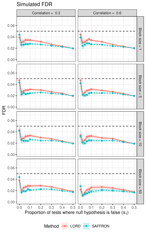
Figure 1: Simulated False Discovery Rates. We generate z-statistics with a block-correlation structure, and generate p-value thresholds based only on the p-values from previous blocks (as in Zrnic et al.,, 2021). Shaded ribbons show $\pm$ 2 Monte Carlo standard errors, defined as $\sqrt{1000^{-1}Var(\text{FDP}(t_{\text{max}}))}$. The dashed line represents our desired alpha level.

6 CONCLUSION

Where SAFFRON, LORD and alpha investing were previously only shown to control FDR under independence, we show that they additionally control FDR under positive, local dependence.

Although our work focuses on controlling FDR, this should not be taken as an implicit, blanket endorsement of FDR over mFDR. On the one hand, Javanmard and Montanari, (2018) argue that FDR carries a more easily understood interpretation than mFDR. On the other, mFDR may be more easily applicable within a decision theory framework (Bickel,, 2004), and may more naturally allow for decentralized control of the proportion of false positives across an entire scientific literature (Fernando et al.,, 2004; see also van den Oord,, 2008; Zrnic et al.,, 2021). Further research into online control for both metrics, as well as control for FWER, remains vital (see also Weinstein and Ramdas,, 2020; Tian and Ramdas,, 2021).

References

- Aharoni and Rosset, (2014) Aharoni, E. and Rosset, S. (2014). Generalized -investing: definitions, optimality results and application to public databases. J. R. Stat. Soc. Series B Stat. Methodol., 76(4):771–794.
- Benjamini and Hochberg, (1995) Benjamini, Y. and Hochberg, Y. (1995). Controlling the false discovery rate: A practical and powerful approach to multiple testing. J. R. Stat. Soc. Series B Stat. Methodol., 57(1):289–300.
- Benjamini and Yekutieli, (2001) Benjamini, Y. and Yekutieli, D. (2001). The control of the false discovery rate in multiple testing under dependency. Ann. Stat., 29(4):1165–1188.
- Bickel, (2004) Bickel, D. R. (2004). Error-rate and decision-theoretic methods of multiple testing: which genes have high objective probabilities of differential expression? Stat. Appl. Genet. Mol. Biol., 3:Article8.
- Chen and Kasiviswanathan, (2020) Chen, S. and Kasiviswanathan, S. (2020). Contextual online false discovery rate control. In Chiappa, S. and Calandra, R., editors, Proceedings of the Twenty Third International Conference on Artificial Intelligence and Statistics, volume 108 of Proceedings of Machine Learning Research, pages 952–961. PMLR.
- Efron and Hastie, (2016) Efron, B. and Hastie, T. (2016). Computer Age Statistical Inference. Cambridge University Press.
- Fernando et al., (2004) Fernando, R. L., Nettleton, D., Southey, B. R., Dekkers, J. C. M., Rothschild, M. F., and Soller, M. (2004). Controlling the proportion of false positives in multiple dependent tests. Genetics, 166(1):611–619.
- Foster and Stine, (2008) Foster, D. P. and Stine, R. A. (2008). -investing: A procedure for sequential control of expected false discoveries. J. R. Stat. Soc. Series B Stat. Methodol., 70(2):429–444.
- Javanmard and Montanari, (2018) Javanmard, A. and Montanari, A. (2018). Online rules for control of false discovery rate and false discovery exceedance. aos, 46(2):526–554.
- Ramdas et al., (2017) Ramdas, A., Yang, F., Wainwright, M. J., and Jordan, M. I. (2017). Online control of the false discovery rate with decaying memory. In Guyon, I., Luxburg, U. V., Bengio, S., Wallach, H., Fergus, R., Vishwanathan, S., and Garnett, R., editors, Advances in Neural Information Processing Systems, volume 30. Curran Associates, Inc.
- Ramdas et al., (2018) Ramdas, A., Zrnic, T., Wainwright, M., and Jordan, M. (2018). SAFFRON: an adaptive algorithm for online control of the false discovery rate. In Dy, J. and Krause, A., editors, Proceedings of the 35th International Conference on Machine Learning, volume 80 of Proceedings of Machine Learning Research, pages 4286–4294. PMLR.
- Storey, (2002) Storey, J. D. (2002). A direct approach to false discovery rates. J. R. Stat. Soc. Series B Stat. Methodol., 64(3):479–498.
- Storey et al., (2004) Storey, J. D., Taylor, J. E., and Siegmund, D. (2004). Strong control, conservative point estimation and simultaneous conservative consistency of false discovery rates: a unified approach. J. R. Stat. Soc. Series B Stat. Methodol., 66(1):187–205.
- Tian and Ramdas, (2019) Tian, J. and Ramdas, A. (2019). ADDIS: an adaptive discarding algorithm for online FDR control with conservative nulls.
- Tian and Ramdas, (2021) Tian, J. and Ramdas, A. (2021). Online control of the familywise error rate. Stat. Methods Med. Res., 30(4):976–993.
- van den Oord, (2008) van den Oord, E. J. C. G. (2008). Controlling false discoveries in genetic studies. Am. J. Med. Genet. B Neuropsychiatr. Genet., 147B(5):637–644.
- Weinstein and Ramdas, (2020) Weinstein, A. and Ramdas, A. (2020). Online control of the false coverage rate and false sign rate. In Iii, H. D. and Singh, A., editors, Proceedings of the 37th International Conference on Machine Learning, volume 119 of Proceedings of Machine Learning Research, pages 10193–10202. PMLR.
- Xu and Ramdas, (2020) Xu, Z. and Ramdas, A. (2020). Dynamic algorithms for online multiple testing.
- Zhang et al., (2020) Zhang, W., Kamath, G., and Cummings, R. (2020). PAPRIKA: Private online false discovery rate control.
- Zrnic et al., (2020) Zrnic, T., Jiang, D., Ramdas, A., and Jordan, M. (2020). The power of batching in multiple hypothesis testing. In Chiappa, S. and Calandra, R., editors, Proceedings of the Twenty Third International Conference on Artificial Intelligence and Statistics, volume 108 of Proceedings of Machine Learning Research, pages 3806–3815. PMLR.
- Zrnic et al., (2021) Zrnic, T., Ramdas, A., and Jordan, M. I. (2021). Asynchronous online testing of multiple hypotheses. J. Mach. Learn. Res., 22:33–31.