ThERESA: Three-Dimensional Eclipse Mapping with Application to Synthetic JWST Data

Abstract

Spectroscopic eclipse observations, like those possible with the James Webb Space Telescope, should enable 3D mapping of exoplanet daysides. However, fully-flexible 3D planet models are overly complex for the data and computationally infeasible for data-fitting purposes. Here, we present ThERESA, a method to retrieve the 3D thermal structure of an exoplanet from eclipse observations by first retrieving 2D thermal maps at each wavelength and then placing them vertically in the atmosphere. This approach allows the 3D model to include complex thermal structures with a manageable number of parameters, hastening fit convergence and limiting overfitting. An analysis runs in a matter of days. We enforce consistency of the 3D model by comparing vertical placement of the 2D maps with their corresponding contribution functions. To test this approach, we generated a synthetic JWST NIRISS-like observation of a single hot-Jupiter eclipse using a global circulation model of WASP-76b and retrieved its 3D thermal structure. We find that a model which places the 2D maps at different depths depending on latitude and longitude is preferred over a model with a single pressure for each 2D map, indicating that ThERESA is able to retrieve 3D atmospheric structure from JWST observations. We successfully recover the temperatures of the planet’s dayside, the eastward shift of its hotspot, and the thermal inversion. ThERESA is open-source and publicly available as a tool for the community.

1 INTRODUCTION

Exoplanet atmospheric retrieval is a method of inferring the temperature and composition of extrasolar planets based on the observed spectrum and photometry. Retrieval can be done in two ways: by modeling planetary emission, measured through direct observation or monitoring flux loss during eclipse, and by modeling the transmission of stellar light through the planet’s atmosphere while the planet transits its host star (e.g., Deming & Seager, 2017). Historically, due to the challenges of observing planets in the presence of much larger, brighter stars, exoplanet retrievals have been limited to measurement of bulk properties, using a single temperature-pressure profile and set of molecular abundance profiles for the entire planet (e.g., Kreidberg et al., 2015; Hardy et al., 2017; Garhart et al., 2018). Analyses like these can be biased, with the retrieved properties possibly not representative of any single location on the planet (Feng et al., 2016; Line & Parmentier, 2016; Blecic et al., 2017; Lacy & Burrows, 2020; MacDonald et al., 2020; Taylor et al., 2020).

Eclipse mapping is a technique for converting exoplanet light curves to brightness maps. During eclipse ingress and egress, the planet’s host star blocks and uncovers different slices of the planet in time. Brightness variations across the planet result in changes in the morphology of the eclipse light curve (Williams et al., 2006; Rauscher et al., 2007; Cowan & Fujii, 2018). HD 189733 b is the only planet successfully mapped from eclipse observations, by stacking many 8.0 µm light curves (de Wit et al., 2012; Majeau et al., 2012). However, with the advent of the James Webb Space Telescope (JWST) in the near future, we expect observations of many more planets to be of sufficient quality for eclipse mapping (Schlawin et al., 2018).

2D eclipse mapping, where a single light curve is inverted to a spatial brightness map, is a complex process. Depending on assumptions about the planet’s structure, retrieved maps can be strongly correlated with orbital and system parameters (de Wit et al., 2012). Rauscher et al. (2018) presented a mapping technique using an orthogonal basis of light curves, reducing parameter correlations and extracting the maximum information possible.

In principle, spectroscopic eclipse observations, like those possible with JWST, should allow 3D eclipse mapping of exoplanets. Every wavelength probes different pressures in the planet’s atmosphere. These ranges depend on the wavelength-dependent opacity of the atmosphere, which in turn depends on the absorption, emission, and scattering properties of the atmosphere’s constituents. Thus, eclipse observations are sensitive to both temperature and composition as functions of latitude and longitude. In practice, however, 3D eclipse mapping is complex. Each thermal map computed from a spectral light curve corresponds to a range or ranges of pressures, which can vary significantly across the planet (Dobbs-Dixon & Cowan, 2017). Unlike 2D mapping at a single wavelength, 3D mapping requires computationally-expensive radiative transfer calculations, which can be prohibitive when exploring model parameter space. Also, the 3D model parameter space is extensive, so one must make simplifying considerations based on the quality of the data.

Mansfield et al. (2020) introduced a method to use clustering algorithms with a set of multi-wavelength maps to divide the planet into several regions with similar spectra. While not a fully-3D model, this method shows promise for distinguishing spatial regions with distinct thermal profiles or chemical compositions, determined from atmospheric retrieval of the individual regions.

In this work we build upon Rauscher et al. (2018), combining eclipse mapping techniques with 1D radiative transfer to present a mapping method that captures the full 3D nature of exoplanet atmospheres while being maximally informative, with constraints to enforce physical plausibility and considerations that improve runtime. In Section 2 we describe our 2D and 3D mapping approaches, in Section 3 we apply our methods to synthetic observations, in Section 4 we compare our retrieved 2D and 3D maps with the input planet model, and in Section 5 we summarize our conclusions.

2 METHODS

Here we present the Three-dimensional Exoplanet Retrieval from Eclipse Spectroscopy of Atmospheres code (ThERESA). ThERESA combines the methods of Rauscher et al. (2018) with thermochemical equilibrium calculations, radiative transfer, and planet integration to simultaneously fit spectroscopic eclipse light curves, retrieving the three-dimensional thermal structure of exoplanets. The code operates in two modes – 2D and 3D – with the former as a pre-requisite for the latter. The code structure is shown in Figure 1, with further description in the following sections. The version of ThERESA used for this analysis can be found at https://doi.org/10.5281/zenodo.5773215.

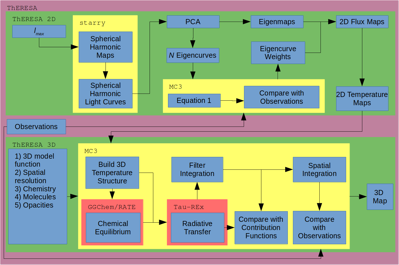
Figure 1: The code structure of ThERESA. The blue boxes show inputs or stages of the analysis, with arrows showing the order of execution. The background colors show which code(s) perform each stage. The steps within the MC3 boxes are run thousands of times by MC3, but the calculations are handled by ThERESA (unless otherwise noted).

2.1 2D Mapping

ThERESA’s 2D mapping follows the methods of Rauscher et al. (2018). First, we calculate a basis of light curves, at the supplied observation times, from positive and negative spherical-harmonic maps $Y^{l}_{m}$, up to a user-supplied complexity $l_{max}$ using the starry package (Luger et al., 2019). These light curves are then run through a principle component analysis (PCA) to determine a new basis set of orthogonal light curves, ordered by total power, which are used in a linear combination to individually model the spectroscopic light curves.

In typical PCA, one subtracts the mean from each observation (spherical-harmonic light curve), computes the covariance matrix of the mean-subtracted set of observations, then calculates the eigenvalues and eigenvectors of this covariance matrix. The new set of observations (“eigencurves”) is the dot product of the eigenvectors and the mean-subtracted light curves, and the eigenvalues are the contributions from each spherical harmonic map to generate each eigencurve. However, the mean-subtraction causes the initial light curve basis set to have non-zero values during eclipse, a physical impossibility that propagates forward to the new basis set of orthogonal light curves. Integrating a map (an “eigenmap”) created from these eigenvalues will not generate a light curve that matches the eigencurves. Therefore, we use truncated singular-value decomposition (TSVD), provided by the scikit-learn package (Pedregosa et al., 2011). TSVD does not do mean-subtraction so the resulting eigencurves have zero flux during eclipse, as expected, which is an improvement over Rauscher et al. (2018). Figure 2 shows an example of the transformation from spherical-harmonic maps and light curves to eigenmaps and eigencurves.

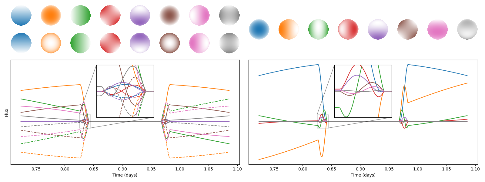
Figure 2: Top Left: The positive and negative spherical harmonic maps with $l\leq 2$, omitting the uniform map $Y^{0}_{0}$. Bottom Left: The secondary-eclipse light curves from integrating the spherical harmonic maps in the top left. Light curve colors match corresponding maps. Dashed lines correspond to negated spherical harmonic maps. Bottom Right: The eigencurves with the eight largest eigenvalues resulting from truncated singular-value decomposition principle component analysis applied to the spherical-harmonic curves in the bottom left. Eigenmaps are ordered, left to right, from most to least information content. Top Right: The eigenmaps corresponding to each eigencurve in the bottom right, with matching colors.

We fit each star-normalized spectroscopic light curve, individually, as a linear combination of $N$ eigencurves, the uniform-map light curve $Y_{0}^{0}$, and a constant offset $s_{corr}$ to account for any stellar flux normalization errors. Each wavelength has its own set of fit values, and potentially its own set of eigencurves, since $N$ and $l_{max}$ can be different for each light curve. Functionally, the model is

$$F_{sys}(t)=c_{0}Y_{0}^{0}+\sum_{i}^{N}c_{i}E_{i}+s_{corr},$$ (1)

where $F_{sys}$ is the system flux, $c_{i}$ are the light-curve weights, and $E_{i}$ are the eigencurves. The light-curve weights and $s_{corr}$ are the free parameters of the model. Although the synthetic data in this work should have $s_{corr}=0$, we still fit to this parameter to better represent an analysis of real data. We run a $\chi^{2}$ minimization to determine the best fit and then run Markov-chain Monte Carlo (MCMC), through MC3 (Cubillos et al., 2017), to fully explore the parameter space.

By construction, the eigenmaps and eigencurves are deviations from the uniform map and its corresponding light curve, respectively, so negative values are possible. If the parameter space is left unconstrained, some regions of the planet may be best fit with a negative flux. To avoid this non-physical scenario, we check for negative fluxes across the visible cells of the planet, based on the times of observation, and penalize the fit. The penalty scales with the magnitude of the negative flux, and we ensure that any negative fluxes result in a worse fit than any planet with all positive fluxes, which effectively guides the fit away from non-physical planets. While the eigenmaps seemingly provide information about the non-visible cells of the planet, these constraints are simply a consequence of the continuity of spherical harmonic maps. Given that we have no real information on those portions of the planet, we do not insist that they have positive fluxes.

We then use the best-fitting parameters with the matching eigenmaps to construct a thermal flux map for the light curve observed at each wavelength (Equation 4 of Rauscher et al., 2018):

$$Z_{p}(\theta,\phi)=c_{0}Y_{0}^{0}(\theta,\phi)+\sum_{i}^{N}c_{i}Z_{i}(\theta,\phi),$$ (2)

where $Z_{p}$ is the thermal flux map, $\theta$ is latitude, $\phi$ is longitude, and $Z_{i}$ are the eigenmaps. These flux maps are converted to temperature maps using Equation 8 of Rauscher et al. (2018):

$$T_{p}(\theta,\phi)=(hc/\lambda k)/\textrm{ln}\left[1+\left(\frac{R_{p}}{R_{s}}\right)^{2}\frac{\exp[hc/\lambda kT_{s}]-1}{\pi Z_{p}(\theta,\phi)(1+s_{corr})}\right],$$ (3)

where $\lambda$ is the band-averaged wavelength of the filter used to observe the corresponding light curve, $R_{p}$ is the radius of the planet, $R_{s}$ is the radius of the star, and $T_{s}$ is the stellar temperature.

When performing 2D mapping, the primary user decisions are choosing $l_{max}$, the maximum order of the spherical harmonic light curves, and $N$, the number of eigencurves to include in the fit. Larger $l_{max}$ (up to a limit) and $N$ result in better fits, as more complex thermal structures become possible. However, these complex planets are often not justified by the quality of the data. To choose $l_{max}$ and $N$ we use the Bayesian Information Criterion (BIC, Raftery, 1995), defined as

$$\textrm{BIC}=\chi^{2}+k\ln n_{data},$$ (4)

where $\chi^{2}$ is the traditional goodness-of-fit metric, $k$ is the number of free parameters in the model ($N+2$ per light curve, assuming a uniform map term $c_{0}$ and $s_{\textrm{corr}}$), and $n_{data}$ is the number of data points being fit. Thus, the BIC penalizes fits which are overly complex. We choose the 2D fit which results in the lowest BIC as the best fit.

2.1.1 Application to Spitzer HD 189733b Observations

To test our implementation of the methods in Rauscher et al. (2018), and the effects of TSVD PCA, we performed the same analysis of Spitzer phase curve and eclipse observations of HD 189733b. The data are the same as those used by Majeau et al. (2012), which include eclipse observations (Agol et al., 2010) and approximately a quarter of a phase curve (Knutson et al., 2007, re-reduced by Agol et al., 2010).

Like Rauscher et al. (2018), we tested a range of values for $l_{\rm max}$ and $N$, using the BIC to choose the model with the highest complexity justified by the data. Table 1 compares our goodness-of-fit statistics with Rauscher et al. (2018). We also determine that the optimal fit uses $l_{\rm max}=2$ and $N=2$ (see figure 3), and our preference for $N=2$ over $N=3$ is stronger. As expected, models with higher $N$ result in lower $\chi^{2}$. For low $N$, we achieve better $\chi^{2}$ and BIC values than Rauscher et al. (2018), although the difference is slight at $N=2$. At higher $N$, differences between the results are statistically negligible. These differences are likely due to the PCA methods used and any differences in the spherical-harmonic light-curve calculation packages used, since Rauscher et al. (2018) employed SPIDERMAN (Louden & Kreidberg, 2018).

Table 1: HD 189733b Goodness-of-fit Statistics

		This work		Rauscher et al. (2018)
$l_{\rm max}$	$N$	$\chi^{2}$	BIC	$\chi^{2}$	BIC
2	1	952.7	973.1	1054	1074
2	2	938.2	965.3	942.4	969.6
2	3	938.0	971.9	938.8	972.7
2	4	937.5	978.2	936.4	977.1
2	5	937.4	984.8	936.4	984.0

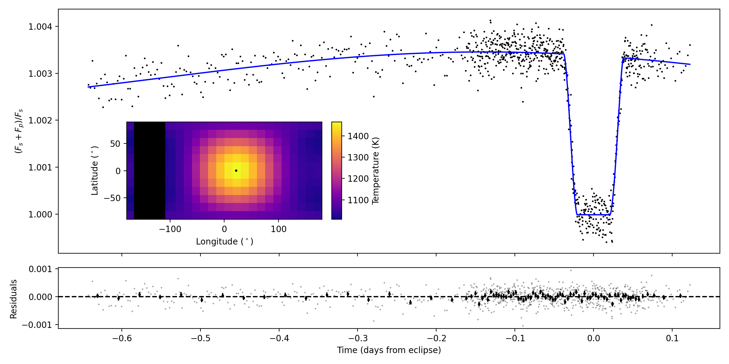
Figure 3: Results of a 2D fit to the HD 189733b Spitzer observations. Top: The light-curve data and best-fitting model. The inset shows the best-fitting thermal map. A black box covers the longitudes not visible during the observations. The hotspot location is marked with a black dot. Bottom: The model residuals and uncertainties. Data are binned for visual clarity, to 10 data points per bin.

Since our eigencurves differ from those used by Rauscher et al. (2018), there is no meaningful comparison between the best-fitting $c_{i}$ parameters. However, the stellar correction $s_{\rm corr}$ has the same function in both works. Notably, we find $s_{\rm corr}=-14\pm 20$ ppm, consistent with zero, whereas Rauscher et al. (2018) find a stellar correction of $452^{+39}_{-40}$ ppm. It is likely that our use of TSVD PCA to enforce zero flux during eigencurve eclipse means the stellar correction term is only correcting for normalization errors, and not also ensuring zero planet flux during eclipse.

To determine the location of the planet’s hotspot, we use starry to find the location of maximum brightness of the best-fit 2D thermal map. Then, to calculate an uncertainty, we repeat this process on 10,000 maps sampled from the MCMC posterior distribution, taking the standard deviation of these locations to be the uncertainty. For HD 189733b, we find a hotspot longitude of $21.8\pm 1.5^{\circ}$ to the east of the substellar point, which very closely matches the $21.6\pm 1.6^{\circ}$ and $21.8\pm 1.5^{\circ}$ found by Rauscher et al. (2018) and Majeau et al. (2012), respectively. Thus, we are confident that we have accurately implemented 2D mapping.

2.2 3D Mapping

Atmospheric opacity varies with wavelength, so spectrosopic eclipse observations probe multiple depths of the planet, in principle allowing for three-dimensional atmospheric retrieval. However, the relationship between wavelength and pressure is very complex. Each wavelength probes a range or ranges of pressures, and those pressures change with location on the planet (Dobbs-Dixon & Cowan, 2017). Here, we combine our 2D maps vertically within an atmosphere, run radiative transfer, integrate over the planet, and compare to all spectroscopic light curves simultaneously with MCMC to retrieve the 3D thermal structure of the planet and parameter uncertainties. We assume that the planet’s atmosphere is static, so that observation time only affects viewing geometry.

The complexity of the radiative transfer calculation and the resulting computation cost forces us to discard the arbitrary resolution of the 2D maps in favor of a gridded planet. The grid size is up to the user (see Section 3.3.2, but smaller grid cells quickly increase mapping runtime.

The 3D planet model is the relationship between 2D temperature maps and pressures. ThERESA offers several such models:

1. “isobaric” – The simplest model, where each 2D map is placed at a single pressure across the entire planet. This model has one free parameter, a pressure (in log space), for each 2D map.

2. “sinusoidal” – A model that allows the pressures of each 2D map to vary as a sinusoid with respect to latitude and longitude. This model has four free parameters for each 2D map: a base pressure, a latitudinal pressure variation amplitude, a longitudinal pressure variation amplitude, and a longitudinal shift, since hot Jupiters often exhibit hotspot offsets. Functionally, the model is:

   $$\log{p(\theta,\phi)}=a_{1}+a_{2}\cos\theta+a_{3}\cos(\phi-a_{4})$$ (5)

   where $a_{i}$ are free parameters of the model. For simplicity, this model does not allow for latitudinal asymmetry, although if the 2D temperature maps are asymmetric in that manner (detectable in inclined orbits), we might expect a similar asymmetry in these pressure maps.

3. “quadratic” – A second-degree polynomial model, including cross terms, for a total of six free parameters. The functional form is:

   $$\begin{split}\log{p(\theta,\phi)}=a_{1}+a_{2}\theta^{2}+a_{3}\theta+\\ a_{4}\phi^{2}+a_{5}\phi+a_{6}\theta\phi\end{split}$$ (6)

   Unlike the isobaric and sinusoidal models, the quadratic model is not continuous opposite of the substellar point, where latitude rolls over from 180^∘ to -180^∘. This is not an issue for eclipse observations, like those presented in this work, but may be problematic if all phases of the planet are visible in an observation. A similar problem occurs at the poles, although these regions contribute very little to the observed flux.

4. “flexible” – A maximally-flexible model that allows each 2D map to be placed at an arbitrary pressure for each grid cell. The number of free parameters is the number of visible grid cells multiplied by the number of 2D maps.

These models represent a range of complexities, and the appropriate function can be chosen using the BIC (Equation 4), assuming that comparisons are made between fits to the same data.

Once the temperature maps are placed vertically, ThERESA interpolates each grid cell’s 1D thermal profile in logarithmic pressure space. The interpolation can be linear, a quadratic spline, or a cubic spline. For pressures above and below the placed temperature maps, temperatures can be extrapolated, set to isothermal with temperatures equal to the closest temperature map, or parameterized, as $T_{top}$ and $T_{bot}$. When parameterized, the top and/or bottom of the atmosphere are given single temperatures across the entire planet and the pressures between are interpolated according to the chosen method. If any negative temperatures are found in the atmosphere grid cells that are visible during the observation, we discard the fit to avoid these non-physical models.

In principle, atmospheric constituents could also be fitted parameters. If the data are of sufficient quality, molecular abundance and temeprature variations across the planet would create observable emission variability depending on the opacity of the atoms and molecules. However, without real 3D-capable data to test against, we assume the planet’s chemistry is in thermochemical equilibrium, with solar atomic abundances. ThERESA offers two ways to calculate thermochemical equilibrium: rate (Cubillos et al., 2019) and GGchem (Woitke et al., 2018). With rate, ThERESA calculates abundances on-the-fly as needed. When using GGchem, the user must supply a pre-computed grid of abundances over an appropriate range of temperatures and at the same pressures of the atmosphere used in the the 3D fit, which ThERESA interpolates as necessary. ThERESA was designed with flexibility in mind, so other abundance prescriptions can be inserted.

Next, ThERESA runs a radiative transfer calculation on each grid cell to compute planetary emission. We use TauREx 3 (Al-Refaie et al., 2019) to run these forward models. Like the atmospheric abundances, the forward model can be replaced with any similar function. We only run radiative transfer (and thermochemical equilibrium) on visible cells to reduce computation time. Spectra are computed at a higher resolution then integrated over the observation filters (“tophat” filters for spectral bins). For computational feasibility, we use the ExoTransmit (Kempton et al., 2017) molecular opacities (Freedman et al., 2008, 2014; Lupu et al., 2014), which have a resolution of 10³, but we note that using high-resolution line lists such as HITRAN/HITEMP (Rothman et al., 2010; Gordon et al., 2017) or ExoMol (Tennyson et al., 2020) would be preferred for accuracy. In this work we use wide spectral bands, which minimizes the effect of using low-resolution opacities.

Finally, we integrate over the planet at the observation geometry of each time in the light curves. The visibility $V$ of each cell, computed prior to modeling to save computation time, is the integral of the area and incident angles combined with the blocking effect of the star, given by

$$V(\theta,\phi,t)=\begin{cases}0&\text{if}\,d<R_{s},\\ \int_{\theta_{i}}^{\theta_{f}}\int_{\phi_{i}}^{\phi_{f}}R_{p}^{2}\cos^{2}\theta^{\prime}\cos\phi^{\prime}d\theta^{\prime}d\phi^{\prime}&\text{otherwise},\\ \end{cases}$$ (7)

where $d$ is the projected distance between the center of the visible portion of a grid cell and the center of the star, defined as

$$\begin{split}d=[(x_{p}+R_{p}\cos\theta\sin\phi-x_{s})^{2}+\\ (y_{p}+R_{p}\sin\theta-y_{s})^{2}]^{1/2}.\end{split}$$ (8)

$x_{p}$ is the $x$ position of the planet, $x_{s}$ is the $x$ position of the star, $y_{p}$ is the $y$ position of the planet, and $y_{s}$ is the $y$ position of the star, calculated by starry for each observation time. These positions include the effect of inclination. We multiply the planetary emission grid by $V$ and sum at each observation time to calculate the planetary light curve. Like the 2D fit, we repeat this process in MCMC to fully explore parameter space. Due to model complexity, traditional least-squares fitting does not converge to a good fit, so we rely on MCMC for both model optimization and parameter space exploration.

2.2.1 Enforcing Contribution Function Consistency

Given absolute freedom to explore the parameter space, the 3D model will often find regions of parameter space which, while resulting in a “good” fit to the spectroscopic light curves, are physically implausible upon further inspection. For instance, the model may bury some of the 2D maps deep in the atmosphere where they have no effect on the planetary emission, or maps may be hidden vertically between other maps, where the combination of linear interpolation and discrete pressure layers causes them to not affect the thermal structure. To avoid scenarios like these, ThERESA has an option where maps are required to remain close (in pressure) to their corresponding contribution functions.

Contribution functions show how much each layer of the atmosphere is contributing to the flux emitted at the top of the atmosphere as a function of wavelength (e.g. Knutson et al., 2009). When integrated over a filter’s transmission curve, they show which layers contribute to the emission in that filter. That is, the contribution function for a given filter shows which pressures of the atmosphere are probed by an observation with that filter. Therefore, a 2D thermal map should be placed at a pressure near the peak contribution, or at least near the integrated average pressure, weighted by the contribution function for the corresponding filter.

To enforce this condition, we apply a penalty on the 3D model’s $\chi^{2}$. For each visible grid cell on the planet, we calculate the contribution function for each filter. We then treat this contribution function, in log pressure space, as a probability density function and compute the 68.3% credible region. Then, we take half the width of this region to be an approximate 1$\sigma$ width of the contribution function, and the midpoint of this region to be the approximate “correct” location for the map. From this width and location, we compute a $\chi^{2}$ for each contribution function and for each grid cell, and add that to the light-curve $\chi^{2}$. We caution that this effectively adds a number of data points equal to the number of visible grid cells, which means BIC comparisons between models that use contribution function fitting and have different grid sizes are invalid.

3 Application to Synthetic WASP-76b Observations

3.1 Light-curve Generation

In lieu of real observations, and as a ground-truth test case, we generated synthetic spectroscopic eclipse light curves of WASP-76b, an ultra-hot Jupiter with a strong eclipse signal. For the thermal structure, we adopt the results of a double-grey general circulation model (GCM, Rauscher & Menou, 2012; Roman & Rauscher, 2017) from Beltz et al. (2021), with no magnetic field. This thermal structure is shown in Figure 4. The GCM output has 48 latitudes, 96 longitudes, and 65 pressure layers ranging from 100 – 0.00001 bar in log space. The double-grey absorption coefficients used in the GCM were chosen to roughly reproduce the average temperature profile for this planet using observational constraints from Fu et al. (2021), which includes a thermal inversion, likely due to TiO in the atmosphere. However, since it is double-gray, the GCM is only using the absorption coefficients to recreate the radiative state of the atmosphere, and is generally agnostic to the atmospheric composition.

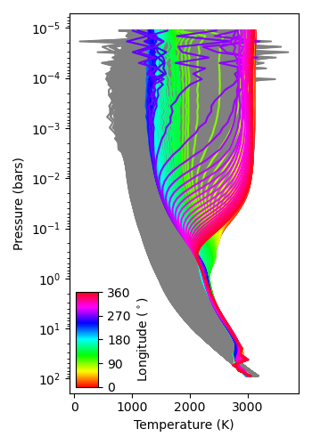
Figure 4: The temperature grid used in light-curve generation. The colored profiles show temperatures at various longitudes along the equator. The substellar point is $0^{\circ}$. All other thermal profiles are plotted in gray.

Since WASP-76b is too hot for rate, we use GGchem to compute molecular abundances. We then use TauREx to calculate grid emission, including opacity from H₂O, CO, CO₂, CH₄, HCN, NH₃, C₂H₂, and C₂H₄, and integrate the planet emission following the visibility function described in Equation 7. The radiative transfer includes no opacity from clouds, because ultra-hot Jupiters are not expected to form clouds, especially on the dayside (Helling et al., 2021; Roman et al., 2021). This is the same process used in the light-curve modeling, except the GCM has a higher grid resolution and the temperatures are set by a circulation model instead of the vertical placement of thermal maps. Our forward model (GCM and radiative transfer) and retrieval do not explicitly include TiO opacity, so our results are still self-consistent with the ground truth.

For the light-curve simulation, we assume the system parameters listed in Table 2. We choose a wavelength range of 1.0 – 2.5 µm, roughly equivalent to the first order of the JWST NIRISS single-object slitless spectroscopy observing mode, a recommended instrument and mode for transiting exoplanet observations. Using the JWST Exposure Time Calculator, we determine the optimal observing strategy is 5 groups per integration, for a total exposure time of 13.30 s. We assume an observation from 0.4 to 0.6 orbital phase with this exposure time for a total of 2352 exposures over 8.69 hours.

Table 2: WASP-76 System Parameters

Parameter	Value
Stellar mass, $M_{s}$	1.46 $M_{\odot}$
Stellar radius, $R_{s}$	1.73 $R_{\odot}$
Stellar temperature, $T_{s}$	6250 K
Planetary mass, $M_{p}$	0.92 $M_{\textrm{J}}$
Planetary radius, $R_{p}$	1.83 $R_{\textrm{J}}$
Orbital period, $P$	1.809866 days
Eccentricity, $e$	0.0
Inclination, $i$	88.0∘
Distance, $D$	195.3 pc

We calculate light-curve uncertainties as photon noise for a single eclipse, assuming a planetary equilibrium temperature of 2190 K. We divide the spectrum into 5 spectral bins of equal size in wavelength space and calculate the photon noise of each bin, assuming Planck functions for planetary and stellar emission. Star-normalized uncertainties range from 26 ppm at 1.14 µm to 55 ppm at 2.35 µm. These are optimistic, uncorrelated uncertainties, but until JWST is operational it is difficult to predict its behavior.

3.2 2D Maps

We fit 2D maps to the synthetic light curves using the methods described in Section 2. Through a BIC comparison between all ($l_{max},N$) pairs for each wavelength, we determine the best $l_{max}$ and $N$ for each light curve (see Table 3). As expected, goodness-of-fit improves as $N$ increases, and reaches a limit where increasing $l_{max}$ no longer improves the fit in a substantial way, once the spherical harmonics capture the observable temperature structure complexity. It is important to fit each light curve with its own $l_{max}$ and $N$; in our case, using a single combination of $l_{max}$ and $N$ results in worse fits (larger BICs) for all five light curves, with a total BIC $\approx$15 higher than the total BIC achieved with individual combinations of $l_{max}$ and $N$.

The four eigenmaps from the fit to the 2.05 µm data, scaled by their best-fitting $c_{i}$ parameters, as well as the scaled uniform map component, are shown in Figure 5. The first eigencurve fits the large-scale substellar-terminator contrast, which is extremely significant for ultra-hot Jupiters and contributes most of the light-curve flux variation, evident in the significant magnitude of the scaled eigenmap. The second eigencurve adjusts for the eastward shift of the planet’s hotspot. The third and fourth curves make further corrections to the temperature variation between the substellar point and the dayside terminators. Eigenmap information content decreases with distance from the substellar point, reaching nearly zero in non-visible portions of the planet, where any variation is only due to the continuity and integration normalization of the original spherical harmonics. Figure 6 shows the light curves at each wavelength, the best-fitting models, and the residuals. Figure 7 shows the best-fitting thermal maps compared with filter-integrated maps of the GCM.

Table 3: 2D Fit BICs

$l_{max}$	$N$	1.14 µm		1.44 µm		1.75 µm		2.05 µm		2.35 µm
		Red. $\chi^{2}$	BIC	Red. $\chi^{2}$	BIC	Red. $\chi^{2}$	BIC	Red. $\chi^{2}$	BIC	Red. $\chi^{2}$	BIC
1	1	2.840	6693.59	3.404	8019.42	4.107	9670.25	3.194	7525.70	3.503	8251.41
1	2	0.995	2367.63	1.138	2702.60	1.077	2558.76	1.031	2451.88	1.045	2484.05
1	3	0.996	2375.45	1.138	2710.44	1.077	2566.49	1.031	2459.67	1.045	2491.97
2	1	2.837	6688.25	3.344	7878.70	4.074	9592.54	3.174	7480.07	3.497	8237.88
2	2	0.977	2325.42	1.012	2406.48	0.986	2346.08	0.972	2312.66	1.008	2398.75
2	3	0.977	2331.34	1.011	2412.64	0.986	2352.35	0.965	2303.82	1.004	2394.72
2	4	0.977	2338.40	1.012	2419.98	0.985	2358.07	0.963	2305.38	1.002	2397.02
2	5	0.977	2344.87	1.011	2425.29	0.984	2362.29	0.958	2299.91	1.000	2398.90
3	1	2.837	6688.27	3.344	7878.49	4.074	9592.37	3.174	7479.63	3.497	8237.61
3	2	0.977	2325.88	1.012	2406.48	0.986	2346.64	0.972	2313.66	1.009	2399.74
3	3	0.977	2332.19	1.010	2409.55	0.985	2351.54	0.960	2292.15	1.002	2390.80
3	4	0.977	2338.15	1.011	2417.44	0.985	2356.39	0.955	2286.45	0.998	2388.35
3	5	0.977	2345.42	1.008	2417.71	0.984	2360.85	0.953	2288.38	0.998	2393.68
4	1	2.838	6688.84	3.346	7882.25	4.074	9593.78	3.176	7483.10	3.498	8240.50
4	2	0.977	2325.51	1.013	2409.68	0.987	2347.56	0.972	2314.35	1.009	2400.42
4	3	0.977	2331.51	1.010	2408.14	0.985	2350.48	0.958	2286.61	1.001	2387.66
4	4	0.977	2338.46	1.010	2415.93	0.985	2357.49	0.954	2284.98	0.999	2389.33
4	5	0.977	2346.11	1.005	2412.12	0.984	2362.43	0.954	2291.29	0.998	2395.44
5	1	2.838	6688.86	3.346	7882.38	4.074	9593.83	3.176	7483.09	3.498	8240.57
5	2	0.977	2325.53	1.013	2409.79	0.987	2347.61	0.972	2314.36	1.009	2400.49
5	3	0.977	2331.53	1.009	2407.95	0.985	2350.36	0.958	2287.06	1.001	2387.66
5	4	0.977	2338.33	1.010	2415.73	0.985	2357.50	0.954	2285.61	0.999	2389.76
5	5	0.977	2345.92	1.005	2412.08	0.985	2363.12	0.955	2292.65	0.999	2396.47

Note. — The optimal fit for each light curve is in black, fits with a $\Delta$BIC $\leq 2$ (model preference $\approx$3:1 or better) are in blue, fits with $2<\Delta$BIC $\leq 5$ (model preference $\approx$3:1 – 10:1) are in orange, and all worse fits are in red. In some cases (e.g., $l_{max}=2,N=2$ and $l_{max}=3,N=2$ for 1.44 µm), the BICs appear to be identical when printed with these digits, but the true best case is in black.

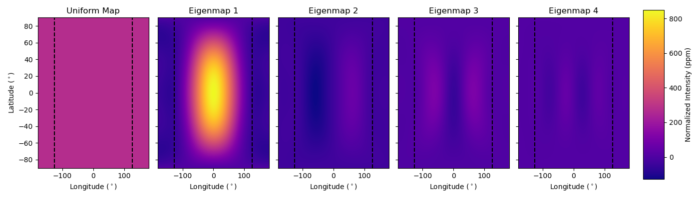
Figure 5: Uniform map and eigenmap components of the 2D fit to the 2.05 µm light curve. The magnitude of each map has been scaled by the best-fitting $c_{i}$ value. The vertical dashed lines denote the minimum and maximum visible longitudes during the observation, at -126^∘ and 126^∘.

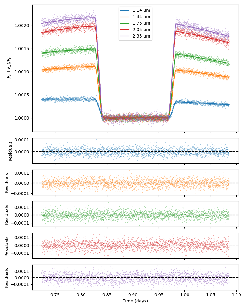
Figure 6: 2D fits to each of the spectroscopic light curves, and the residuals.

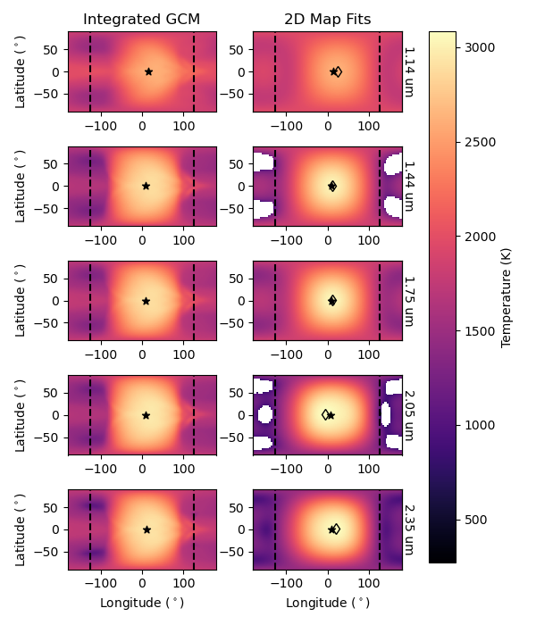
Figure 7: Comparison between input thermal maps and retrieved 2D maps. Dashed lines indicate the edges of the visible portion of the planet. The GCM hotspot location (see main text) is marked with a star and the fitted hotspot location is marked with a diamond. Left: Thermal maps from the GCM, computed using filter-integrated flux maps and Equation 3. Right: 2D thermal maps derived from fits to each light curve. The maps are plotted at the resolution of the GCM, but these maps can be computed at an arbitrary resolution. The blank spaces have undefined temperatures, as the 2D fit produces negative flux in those regions. This is permitted because those grid cells are never visible during the observation, so we formally have no information about them.

3.3 3D Map

As described above, we fit a 3D model to the spectroscopic light curves by placing 2D maps vertically in the atmosphere, interpolating a 3D temperature grid, computing thermochemical equilibrium of the 3D grid, calculating radiative transfer for each planetary grid cell, and integrating over the planet for the system geometry of each exposure in the observation.

Since WASP-76b is an ultra-hot Jupiter (zero-albedo, instantaneous redistribution equilibrium temperature of 2190 K), we use GGchem to calculate thermochemical equilibrium abundances. As with the light-curve generation, the radiative transfer includes H₂O, CO, CO₂, CH₄, HCN, NH₃, C₂H₂, and C₂H₄ opacities, all from ExoTransmit. The atmosphere has 100 discrete layers, evenly spaced in logarithmic pressure space, from $10^{-6}$ – $10^{2}$ bar.

3.3.1 Spectral Binning

With spectroscopic observations, the spectral binning is up to the observer. This choice is far from simple. Smaller bins lead to a better-sampled spectrum, and each wavelength bin likely probes a smaller range of pressures, potentially allowing for better characterization of the atmosphere, as the atmosphere is less likely to be well fit with all maps placed at similar pressures. However, small wavelength bins lead to more uncertain light curves and, thus, more uncertain 2D maps to use in the 3D retrieval. Since we do not incorporate the uncertainty of the 2D maps in our 3D retrieval (aside from adjusting their positions vertically), we take the cautious approach of minimizing this uncertainty by using only five evenly-spaced spectral bins from 1.0 – 2.5 µm.

3.3.2 Planet Grid Size

Our formulation of the visibility function (Equation 7), counts planet grid cells as either fully visible or obscured depending on the position of the center of the grid cell relative to the center of the projected stellar disk. This approximation approaches a smooth eclipse for infinitely small grid cells, but 3D model calculation time scales approximately proportionally to the number of grid cells, quickly becoming infeasible. Therefore we must choose a planetary grid resolution that adequately captures the eclipse shape within observational uncertainties and keeps model runtime manageable. Figure 8 compares uniformly-bright WASP-76b eclipse ingress models for a range of grid resolutions with the analytic ingress model. At a resolution of $15^{\circ}\times 15^{\circ}$, the deviations from the analytic model are within the 1$\sigma$ region for the filter which yields the highest signal-to-noise ratio, so we adopt this grid resolution.

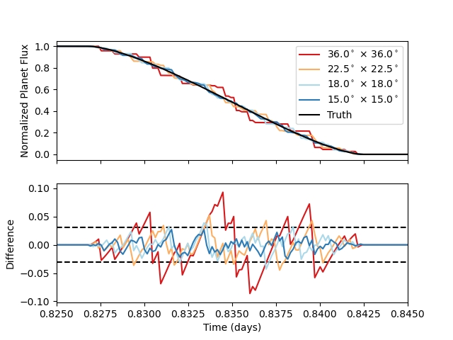
Figure 8: Top: The normalized ingress of a uniformly-bright WASP-76b, computed by integrating the planet with the visibility function (Equation 7) for a range of grid sizes, compared to the true ingress shape computed analytically with starry. Bottom: The difference between the true ingress and the gridded planets. The dashed lines indicate the normalized 1$\sigma$ region for the highest signal-to-noise filter in our synthetic observation of WASP-76b. The light curve of a sufficiently high-resolution grid should fall within these boundaries.

3.3.3 Temperature-Pressure Interpolation

By default, ThERESA uses linear interpolation, in log-pressure space, to fill in the temperature profiles between the 2D maps. Since the atmosphere is discretized into pressure layers, if $>2$ thermal maps are placed between two adjacent pressure layers for a given grid cell, the grid cells of the central maps of this grouping have no effect on the 3D thermal structure. This problem is significantly exacerbated when using the isobaric pressure mapping method, where entire 2D maps, rather than just a single cell of a map, can be hidden.

We experimented with quadratic and cubic interpolation to mitigate this problem, as those methods make use of more than just the two adjacent thermal maps nearest to the interpolation point. However, these interpolation methods cause significant unrealistic variation in the vertical temperature structure, often creating negative temperatures, artificially limiting parameter space (as these negative temperature models are rejected). Therefore, we elect to use linear interpolation and rely on the contribution function constraint (see Section 2.2.1) to guide the 2D thermal maps to consistent pressure levels. While it is still possible to hide maps, for a good fit this will only happen when maps have similar temperatures.

3.3.4 Pressure Mapping Function

We tested each of the pressure mapping functions described in Section 2.2 – isobaric, sinusoidal, quadratic, and flexible – to determine which is most appropriate for our synthetic WASP-76b observation. For all four cases, we use an additional parameter to set the planet’s internal temperature (at 100 bar) but leave the upper atmosphere to be isothermal at pressures lower than the highest 2D map in each grid cell.

The isobaric model, which contains only 6 free parameters – a pressure level for each 2D temperature map and an internal temperature – fits the data quite well. We achieve a reduced $\chi^{2}$ of 1.067 and a BIC of 13750.55, including the penalty for contribution function fitting. The fit places the 2D maps for the four longest wavelengths, which all have similar temperatures, at $\approx 0.05$ bar and puts the 1.14 µm map slightly deeper, at $\approx 0.08$ bar, creating the temperature inversion seen in the GCM (see Figure 4). Figure 9 shows the 3D temperature structure, with each profile weighted by the contribution functions of each filter in each grid cell.

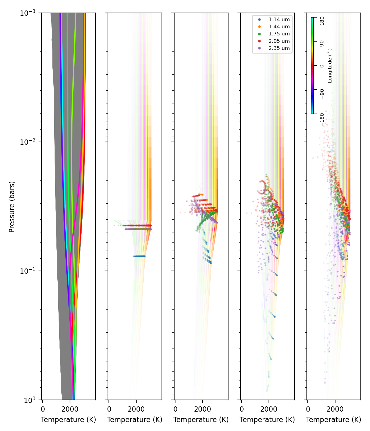
Figure 9: Left to right: the input temperature grid from the GCM, the isobaric retrieval, the fixed-phase sinusoidal retrieval, the free-phase sinusoidal retrieval, and the quadratic retrieval. The colored lines indicate temperature profiles along the equator, with the GCM downsampled to the spatial resolution of the fitted temperature grid. All others are plotted in gray. For the fitted grid, plotted color opacity for each profile is weighted by the maximum contribution function (over all filters) for each grid cell and pressure layer, normalized to the largest contribution. Non-visible grid cells have a contribution of 0. Dots indicate the placement of the 2D temperature maps for each (visible) grid cell, and their plotting opacity is the ratio of the total contribution from that grid cell and filter to the maximum total contribution.

The sinusoidal pressure mapping function will always result in a fit at least as good as the isobaric model, as there is a set of sinusoidal model parameters that replicates the isobaric model, but the additional complexity may not be justified by the quality of our data. Here, however, we find a significant improvement. First, we use the sinusoidal function but fix the phase of the longitudinal sinusoid ($a_{4}$ in Equation 5) equal to the hotspot longitude, effectively assuming the contribution function variation follows temperature variation. With this parameterization, we find a reduced $\chi^{2}$ of 1.013 and a BIC of 13142.84.

If we also allow the $a_{4}$ terms to vary, the sinusoidal model is no longer forced to tie the hottest part of each 2D map to the highest or lowest pressure of that map’s vertical position. This added flexibility improves the fit to a reduced $\chi^{2}$ of 0.989 and a BIC of 12879.60. Looking at Figure 9, we see that the hottest portion of 1.75 µm 2D map is shifted to higher pressures and the 1.14 µm map is pushed deeper, smoothing out the temperature inversion.

The quadratic model is the next step up in complexity. With this model, we achieve a reduced $\chi^{2}$ of 1.037 and a BIC of 13580.20. This is a worse fit than the sinusoidal models, and a much higher BIC, suggesting that the sinusoidal model better captures the 3D placement of the 2D maps using fewer free parameters.

We also tested the “flexible” 3D model. With 12 latitudes and 24 longitudes, and a visible range of $\phi\in(-126^{\circ},126^{\circ})$, there are 216 visible and partially-visible grid cells. With 5 wavelength bins and an internal temperature parameter, there are 1081 model parameters in total (including the internal temperature). In a best-case scenario, we would achieve a reduced $\chi^{2}$ of 1, implying a BIC $\geq 21882.26$, far greater than the BICs we achieve with simpler, less flexible models. Without a drastic reduction in observational uncertainties, the data are unable to support such a model. In fact, such a reduction in light-curve uncertainties would require a finer planetary grid (see Section 3.3.2), in turn requiring additional parameters, further increasing the BIC and decreasing preference for this model.

As with choosing $N$ in the 2D mapping, we use the BIC to determine the optimal 3D model. For these data, we achieve the lowest BIC using the free-phase sinusoidal model.

3.4 Credible Region Errors

To assess the completeness of the MCMC parameter-space exploration, we compute the Steps Per Effectively Independent Sample (SPEIS), Effective Sample Size (ESS), and the absolute error on our 68.3% (1$\sigma$) credible region $\sigma_{C}$ of our posterior distribution following Harrington et al. (2021). We compute SPEIS using the initial positive sequence estimator (Geyer, 1992), then divide the total number of iterations by the SPEIS to calculate ESS. Then,

$$\sigma_{C}=\sqrt{\frac{C(1-C)}{{\rm ESS}+3}},$$ (9)

where $C=0.683$ is a given credible region. We calculate an ESS for each parameter of each chain and sum over all chains to get a total ESS.

4 Discussion

4.1 2D Thermal Maps

From a qualitative perspective the retrieved maps match the GCM well. Figure 7 shows a comparison of the 2D thermal maps extracted from the GCM used to generate the light curves and the retrieved maps. Large-scale features, like the planet’s hotspot and its eastward shift from the substellar point are recovered. As expected, there is little match between the night side of the GCM and the fitted maps, and the fits are often non-physical in this region, as we do not apply physicality constraints to non-visible portions of the planet. The fits are also unable to recover smaller-scale features, like the latitudinal width of the equatorial jet and the sharp drops in temperature near the planet’s terminator, which cannot be replicated without many additional eigencurves.

From the MCMC parameter posterior distribution, we can generate a posterior distribution of maps to examine a variety of features. By finding the maximum of a subsample of 10,000 maps in the posterior distribution, we can identify the location and uncertainty of the planet’s hotspot and determine if there is a longitudinal shift from the substellar point, a useful metric for understanding the dynamics of the planet’s atmosphere. For WASP-76b, we determine hotspot longitudes of $23.8^{+1.1}_{-1.2}$, $11.4^{+0.3}_{-0.1}$, $12.4^{+0.3}_{-0.3}$, $-4.9^{+4.8}_{-4.2}$, and $20.8^{+3.6}_{-4.5}$ degrees for each bandpass in increasing wavelength, respectively (see Figure 10). For comparison to the GCM, we constructed 1D cubic splines along the equators of the GCM temperature maps (Figure 7) and found their maxima. The GCM has hotspot longitudes of $14.1^{\circ}$, $9.1^{\circ}$, $9.2^{\circ}$, $7.8^{\circ}$, and $10.1^{\circ}$. In a broad sense, our 2D retrieval captures the stronger eastward shift at 1.14 µm and places the other 4 maps closer together, much like the GCM maps. Differences are likely due to the limited temperature structures possible with $N\leq 4$ fits and approximating the GCM hotspot as the equatorial longitude with the peak temperature. Unsurprisingly, the fitted hotspot latitudes are very near the equator, since none of the included eigenmaps contain significant north-south variation, which should be detectable for orbits with non-zero (but less than $1-R_{p}/R_{s}$) impact parameters.

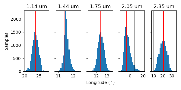
Figure 10: Histograms of hotspot longitude from the MCMC posterior distributions for each 2D map. The best-fitting hostpot longitude is overplotted in a red line. The GCM hotspot longitude is shown with a black line if it falls within the longitudes of the $x$-axes.

Using the subsample of posterior maps, we also can calculate uncertainties on the temperature maps, at arbitrary resolution, by evaluating the standard deviation of the temperature in each grid cell. Figure 11 shows the full temperature uncertainty maps and equatorial profiles. Uncertainties are low, at $\approx 10$ K, for grid cells that are visible throughout the observation. Grid cells at higher longitudes are less well constrained because 1) they are only visible or partially visible for a portion of the observation, and 2) they contribute less to the planet-integrated flux due to the visibility function (Equation 7). Likewise, high latitudes are less well constrained.

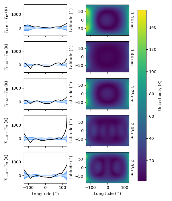
Figure 11: Uncertainties in the 2D temperature map fits, calculated as the standard deviation of the posterior distribution of maps. Plots are at the spatial resolution of the GCM, although they can be computed at any resolution. Axes are limited to locations visible during the observation. Left: Difference between the GCM (in black) and fitted equatorial temperatures. The shaded regions denote the 1$\sigma$, 2$\sigma$, and 3$\sigma$ boundaries. Right: Temperature uncertainty maps, calculated as the standard deviation at each location.

While the thermal maps agree with the GCM at many locations on the planet, there are a few places where the discrepancy is significant within the uncertainties. In several bandpasses we overestimate the temperature of the hotspot, four of the maps overestimate the temperature of the western terminator, and all five maps underestimate temperatures at the extreme ends of the visible longitudes. These discrepancies can all be explained by the simplicity of the 2D model, which only contains two to four statistically-justified eigencurves. The model cannot capture the fine details of the GCM thermal structure, and the uncertainties are likewise constrained. Indeed, if we increase the number of eigencurves, we both improve the match with the GCM and increase the temperature uncertainties to encompass the difference between the fit and truth (see Figure 12). However, this also significantly increases the uncertainty on the location of the planet’s hotspot and the additional parameters are not statistically justified, evident in the minor changes to the best fit as more parameters are introduced. For example, adding only one more eigencurve to the 1.14 µm fit ($N=3$) increases the BIC by $5.92$ (Table 3), a preference for the $N=2$ model of $\approx$19:1. This figure also shows the fraction of the observation where each equatorial longitude is visible, which highlights the correlation between the observability of a location on the planet and the uncertainty on the retrieved temperature of that location. When interpreting analyses of real data we must be aware of these limitations.

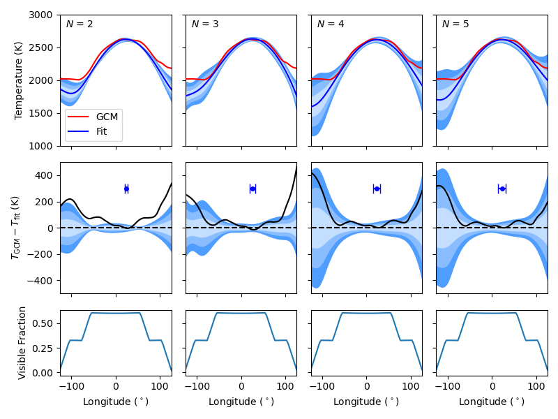
Figure 12: A comparison of the equatorial temperature uncertainties on 1.14 µm maps retrieved with different numbers of eigencurves. The blue region denotes 1, 2, and 3$\sigma$. Only visible longitudes are shown. Top: The equatorial temperatures of the GCM and the best fit. Middle: The difference between the GCM and fitted equatorial temperatures. The blue data point shows the best-fit hotspot longitude and its 3$\sigma$ uncertainty ($y$ location arbitrary). Bottom: The fraction of the observation during which a given longitude, along the equator, is visible to any degree, including the effects of both planet rotation and the occultation by the star. The plateau centered on $0^{\circ}$ shows the longitudes which are visible for the whole observation, except during eclipse. The smaller plateaus near $-90^{\circ}$ and $90^{\circ}$ are the longitudes visible for the entirety of pre- or post-eclipse but not vice versa due to planet rotation during eclipse.

4.2 3D Retrieval

At first glance, the best-fitting 3D models all appear to be physically unrealistic, with internal temperatures at $\approx 500$ K, much lower than the GCM internal temperature of $\approx 3000$ K. However, if we examine the contribution functions of the best-fitting model (shown in line opacity in Figure 9), we see that our spectral bins are primarily sensitive to pressures from 0.001 – 1 bar, and the majority of the emitted flux comes from the hottest grid cells at pressures between 0.01 and 0.1 bar, far from the interior of the planet at 100 bar. Therefore, the internal temperature parameter is only affecting the emitted flux by controlling the temperature gradient near the deepest thermal map, and the absolute value of the parameter is unimportant. In all our fits, this extends the thermal inversion to the deepest visible pressure layers, consistent with the thermal inversion in the GCM, which continues down to $\approx 0.5$ bar at the substellar point. The temperature structure as a whole is physically implausible at higher pressures, but the portions sensed by the observation are reasonable and similar to the GCM. We note that our MCMC analyses started from a more plausible internal temperature of 3000 K, using a uniform prior over the range [0, 4000] K, but without wavelengths which probe the deep atmosphere, those fits were quickly ruled out in favor of the fits presented here.

To further understand the effects of the $T_{bot}$ parameter, we examined the thermal profiles in the MCMC posterior as a function of $T_{bot}$. First, we looked for potential correlations between $T_{bot}$ and the location of the thermal inversion, measured by evaluating the 3D thermal profiles at high vertical (pressure) resolution and finding the pressure level where the temperature gradient becomes negative. This relationship, for the substellar point, is shown in Figure 13, which shows a minor positive correlation, although the variation in the inversion pressure is small. Thus, the $T_{bot}$ parameter is not affecting the location of the thermal inversion.

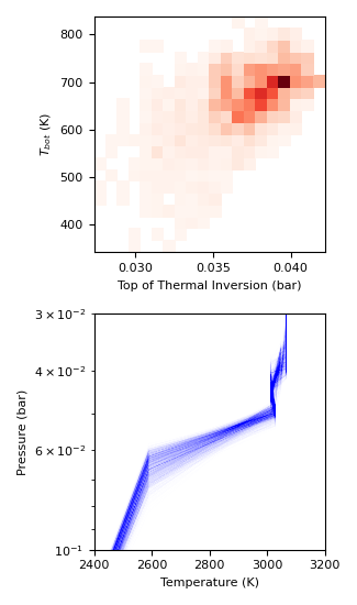
Figure 13: MCMC posterior distribution of temperature profiles at the substellar point, showing our parameterization scheme is not influencing the location of the thermal inversion. For computational feasibility, we thinned the posterior distribution by a factor of 100. Top: The minor positive correlation between $T_{bot}$ and the pressure at the top of the thermal inversion, where the temperature gradient becomes negative. Bottom: The distribution of temperature-pressure profiles in the MCMC posterior near the thermal inversion at the substellar point. At lower pressures the atmosphere is isothermal and at higher pressures the linear trend continues down to $T_{bot}$ at 100 bar.

There are many similarities between the isobaric fit and the two sinusoidal fits. In all cases, the 1.14 µm temperature map is placed at higher pressures than the others to create the thermal inversion near 0.04 bar and the planet has a low internal temperature to continue the temperature inversion. The upper atmosphere is roughly the same, especially in the hottest grid cells. However, while the isobaric model is forced to place all maps near their peak contributions at the planet’s hotspot, the additional flexibility of the sinusoidal model allows the temperature maps to better match their contribution functions (and the emitted spectra) across the entire planet. This is evident in the significantly improved $\chi^{2}$ and BIC. We take the free-phase sinusoidal model to be the optimal fit.

Figure 14 shows the optimal 3D model fit to the light curves, and Table 4 lists the model parameters with their 1$\sigma$ credible regions, SPEIS, ESS, and $\sigma_{C}$, from a 28-day run with $\approx 810,000$ iterations over 7 Markov chains. We discard the first 80,000 iterations of each chain, as the $\chi^{2}$ was still improving significantly, so these iterations are not representative of the true parameter space. These parameters give information about the pressures probed by each filter, as follows: $a_{1}$ is the average logarithmic pressure probed by the corresponding temperature map; $a_{2}$ is the change in logarithmic pressure probed from the equator to the poles; and $a_{3}$ is a similar change from the longitude $a_{4}$ to $a_{4}$ + 180^∘. However, one must keep in mind that the observation is not sensitive to all longitudes, so the $a_{3}$ parameter should only be considered representative of the longitudinal change in probed pressure within the range of visible longitudes (-126^∘ to 126^∘ for this observation).

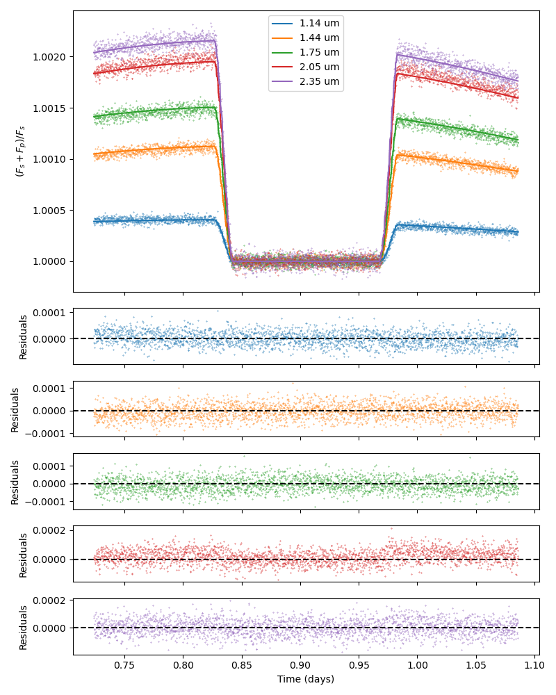
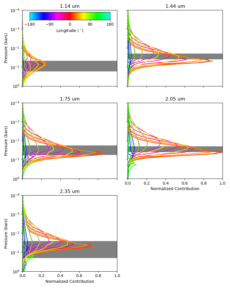
Figure 14: Left: The light-curve fit from the best-fitting 3D model, and the residuals. Right: Contribution functions, normalized to the maximum contribution, for visible grid cells along the equator in the best-fitting 3D model. Each panel shows a different filter. The gray boxes indicate the range of pressures covered by the respective 2D map.

Table 4: Free-phase Sinusoidal 3D Model Parameters

Name	Best fit	$C=0.683$	SPEIS	ESS	$\sigma_{C}$
1.14 µm
$a_{1}$	-0.68	[-0.87, -0.61]	5656	143.2	3.8%
$a_{2}$	0.05	[-0.06, 0.17]	6586	123.0	4.1%
$a_{3}$	0.65	[0.45, 0.67]	11708	69.2	5.5%
$a_{4}$ (∘)	159	[153, 161]	10720	75.6	5.2%
1.44 µm
$a_{1}$	-1.73	[-1.78, -1.67]	5972	135.7	4.0%
$a_{2}$	0.33	[0.30, 0.44]	5907	137.2	3.9%
$a_{3}$	-0.05	[-0.04, -0.00]	21794	37.2	7.3%
$a_{4}$ (∘)	109	[20, 127]	23214	34.9	7.6%
1.75 µm
$a_{1}$	-1.69	[-1.73, -1.62]	5389	150.3	3.8%
$a_{2}$	0.29	[0.21, 0.35]	5867	138.1	3.9%
$a_{3}$	0.11	[0.09, 0.13]	7082	114.4	4.3%
$a_{4}$ (∘)	-23	[-25, -11]	13547	59.8	5.9%
2.05 µm
$a_{1}$	-1.69	[-1.69, -1.57]	6750	120.0	4.2%
$a_{2}$	0.28	[0.15, 0.29]	6436	125.9	4.1%
$a_{3}$	-0.05	[-0.05, -0.02]	11513	70.4	5.4%
$a_{4}$ (∘)	95	[65, 98]	19405	41.7	7.0%
2.35 µm
$a_{1}$	-1.43	[-1.51, -1.33]	8576	94.5	4.7%
$a_{2}$	0.22	[0.10, 0.26]	6472	125.2	4.1%
$a_{3}$	-0.23	[-0.25, -0.15]	10128	80.0	5.1%
$a_{4}$ (∘)	39	[32, 42]	15364	52.7	6.2%
$T_{{bot}}$ (K)	701	[619, 737]	6137	132.0	4.0%

Since the noise in the observation is purely uncorrelated, we can easily see where the model fails to match the observation. There is a minor negative slope in the residuals at 1.14 µm, indicating extra flux east of the substellar point and a flux deficiency west of the substellar point, at those wavelengths. This agrees with the more eastern hotspots found in our 2D maps. Our best fit also produces slightly less flux in the 2.05 µm band than the GCM. All these differences are well within the uncertainties, however, as indicated by the low $\chi^{2}$. Increasing $N$ in the 2D fit could allow for fine adjustment of the 3D thermal structure and improve the 3D fit in these areas, but, as discussed above, additional free parameters are not justified by the data uncertainties. Fits using the simpler pressure-mapping functions have slightly stronger variations in the residuals, but very similar shapes (e.g., a stronger slope at 1.14 µm).

This figure also shows a comparison between the 3D model contribution functions and the vertical placement of the 2D thermal maps, to examine the effectiveness of our contribution function consistency requirement (Section 2.2.1). The range of vertical placement of the 2D thermal maps (gray boxes) align well with the peaks of the contribution functions, demonstrating that our $\chi^{2}$ penalty is successfully guiding the fit to a consistent result. Figure 15 shows a comparison of the equatorial contribution functions with the 2D map placements overlaid, which confirms that the 2D maps’ vertical position matches the contribution functions, especially for the hottest grid cells.

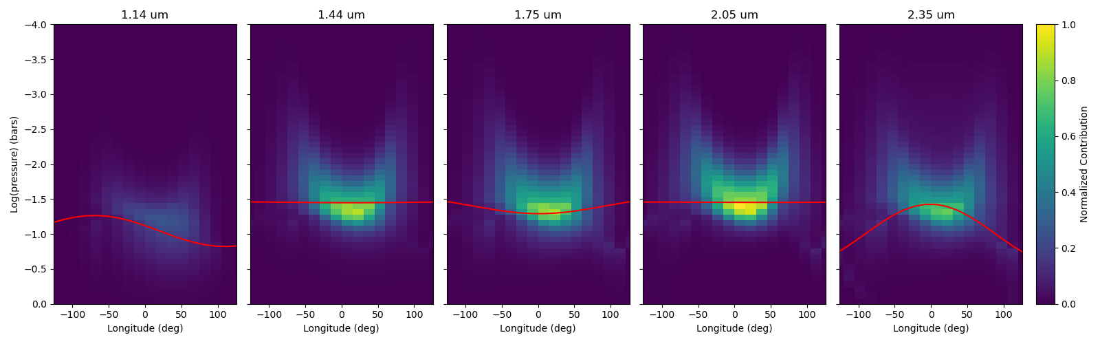
Figure 15: The normalized equatorial contribution functions for each spectroscopic bin. The vertical, equatorial placements of the 2D thermal maps from the optimal fit of the free-phase sinusoidal function (Table 4) are overplotted in red.

Uncertainties on the placement of the 2D maps are straightforward to evaluate, using the marginalized MCMC posterior distributions. For instance, for the isobaric model, the 2D maps are placed, in order of increasing wavelength, at $-1.115^{+0.006}_{-0.014}$, $-1.326^{+0.004}_{-0.017}$, $-1.325^{+0.011}_{-0.001}$, $-1.353^{+0.010}_{-0.023}$, and $-1.326^{+0.005}_{-0.014}$ log(bar pressure), with an internal temperature of $630^{+64}_{-38}$ K. The uncertainties on these model parameters, and those of the other 3D model functions, can be lower than the model’s vertical resolution since the discretized layers of the model have temperatures interpolated from the vertical placement of the 2D temperature maps. The 2D maps can be placed anywhere within the pressure range of the model, and are not restricted to the precise layering of the model.

However, uncertainties on the 3D temperature model as a whole are more nuanced. A distribution of 3D models generated from the MCMC parameter posterior distribution will lead one to believe the atmosphere is very well constrained. However, much like the uncertainties on the 2D models are restricted by the flexibility of the eigenmaps, uncertainties on the best-fitting 3D models are restricted by the models’ functional forms. Additionally, the uncertainties on the 2D maps are not propagated to the 3D fits. The upper atmosphere will appear constrained to absolute certainty because the model sets these temperatures to be isothermal with the lowest-pressure 2D map in each grid cell. Therefore, temperatures at these low pressures do not vary in the MCMC unless the 2D maps are swapping positions, and even then the upper atmosphere of each grid cell can only have a number of unique temperatures equal to the number of 2D maps present. For pressures between 2D map placements, the temperature profile interpolation and vertical shifting of the 2D maps leads to a range of temperatures in the posterior distribution of models, but variation is still significantly limited by the temperatures present in the 2D maps. At higher pressures, temperatures are strongly tied to the deepest 2D map but some variation is allowed by the internal temperature parameter. Uncertainties on the 3D model are much better understood by studying the contribution functions, as uncertainties should be considered unconstrained in portions of the atmosphere with zero contribution to the planet’s flux.

4.2.1 Thermal Inversion

The presence of strong optical absorbers, such as TiO, is often invoked to explain the presence of thermal inversions, as this molecule can significantly heat a planet’s upper atmosphere (Hubeny et al., 2003; Fortney et al., 2006, 2008). Evidence of TiO has been found in observations of multiple hot Jupiters (e.g., Kirk et al., 2021; Changeat & Edwards, 2021), including WASP-76b (Fu et al., 2021).

Both our radiative transfer forward model of the ground truth and the retrieved 3D model do not include TiO, and yet we retrieve the input thermal inversion. As described in Section 3, the temperature inversion in the GCM is produced by the relative ratio between the infrared and optical absorption coefficients, which are broadband and do not include molecular spectral absorption (such as by TiO). The retrieval framework does not require TiO, but for a different reason; the temperature profiles are entirely parameterized and so do not require a physical heating mechanism to produce an inversion. This is a strength of the model, as real exoplanet atmospheres are likely in complex thermal states which can, in principle, be recreated by our model.

While we achieve an excellent fit to the eclipse spectra without TiO, it is possible that the inclusion of this molecule would affect the emission spectra enough to shift the pressures probed by our observations, changing the optimal locations of the 2D temperature maps. However, TiO opacity peaks in the optical and falls off rapidly into the near-infrared wavelengths (e.g., Gharib-Nezhad et al., 2021). Thus, the impact on our models should be small.

5 Conclusions

In preparation for the 3D exoplanet mapping capabilities of JWST, we have presented the ThERESA code, a fast, public, open-source package for 3D exoplanet atmosphere retrieval. The code builds upon the maximally-informative 2D mapping techniques of Rauscher et al. (2018) with the addition of 3D planet models, composition calculations, radiative transfer computation, and planet integration to model observed eclipse spectra. Thus, we combine a 2D mapping scheme with 1D radiative transfer into a 3D model with a manageable number of parameters, enabling fast fit convergence. For example, the isobaric model, running on 11 processors and $<5$ gigabytes of memory, with 12 latitudes, 24 longitudes, 100 pressure layers, and eight molecules, converges in $<3$ days of runtime. More complex models can take a few weeks depending on the desired error level in the parameter credible regions.

ThERESA improves upon the 2D mapping methods of Rauscher et al. (2018) by (1) using TSVD PCA to ensure that eigencurves have the expected zero flux during eclipse, reducing the need for a stellar correction term, and (2) restricting parameter space to avoid non-physical negative fluxes at visible locations on the planet, forcing positive temperatures and enabling radiative transfer calculations. Through a reanalysis of Spitzer HD 189733 b observations, we demonstrated the accuracy of ThERESA’s implementation of 2D eigencurve mapping. Our measurement of the eastward shift of the planet’s hotspot agrees extremely well with previous studies (Majeau et al., 2012; Rauscher et al., 2018).

Our 3D planet models consist of functions which attach 2D maps to pressures that can vary by position on the planet, using functions which range in complexity from a single pressure per map to a maximally-flexible model with a parameter for the vertical position of every 2D map in every grid cell. We also require that 2D maps be placed near the peaks of their corresponding contribution functions, ensuring consistency between the 3D model and the radiative transfer calculations.

To test the accuracy of our retrieval method, and to explore the capabilities of eclipse mapping with JWST, we generated a synthetic eclipse observation from WASP-76b GCM results. Our 2D maps are able to retrieve the large-scale thermal structure of the GCM with $l_{\rm max}\leq 5$ and $N\leq 4$, the highest-complexity fits justified by a BIC comparison. We caution that the limited complexity of the eigencurves and eigenmaps limits the structures possible in the best-fitting maps and their uncertainties. Future mapping analyses must be cognizant of these limitations when presenting results.

Our 3D retrievals, regardless of the temperature-to-pressure model used, were able to accurately determine the temperatures of the planet’s atmosphere that we are sensitive to, from $\sim 0.001-0.1$ bar, including the presence of a thermal inversion at the planet’s hotspot near 0.04 bar, while maintaining a radiatively consistent atmosphere by ensuring that 3D model contribution functions match the vertical placements of the 2D temperature maps. Through a BIC comparison, a sinusoidal model function that includes combined latitudinal, longitudinal, and vertical information was preferred over a purely isobaric model, demonstrating that 3D models are necessary to interpret JWST-like observations, and ThERESA can perform the analyses on such data.

References

- Agol et al. (2010) Agol, E., Cowan, N. B., Knutson, H. A., et al. 2010, ApJ, 721, 1861, doi: 10.1088/0004-637X/721/2/1861
- Al-Refaie et al. (2019) Al-Refaie, A. F., Changeat, Q., Waldmann, I. P., & Tinetti, G. 2019, arXiv e-prints, arXiv:1912.07759. https://arxiv.org/abs/1912.07759
- Beltz et al. (2021) Beltz, H., Rauscher, E., Roman, M., & Guilliat, A. 2021, arXiv e-prints, arXiv:2109.13371. https://arxiv.org/abs/2109.13371
- Blecic et al. (2017) Blecic, J., Dobbs-Dixon, I., & Greene, T. 2017, ApJ, 848, 127, doi: 10.3847/1538-4357/aa8171
- Changeat & Edwards (2021) Changeat, Q., & Edwards, B. 2021, ApJ, 907, L22, doi: 10.3847/2041-8213/abd84f
- Cowan & Fujii (2018) Cowan, N. B., & Fujii, Y. 2018, Mapping Exoplanets, ed. H. J. Deeg & J. A. Belmonte, 147, doi: 10.1007/978-3-319-55333-7_147
- Cubillos et al. (2017) Cubillos, P., Harrington, J., Loredo, T. J., et al. 2017, AJ, 153, 3, doi: 10.3847/1538-3881/153/1/3
- Cubillos et al. (2019) Cubillos, P. E., Blecic, J., & Dobbs-Dixon, I. 2019, ApJ, 872, 111, doi: 10.3847/1538-4357/aafda2
- de Wit et al. (2012) de Wit, J., Gillon, M., Demory, B. O., & Seager, S. 2012, A&A, 548, A128, doi: 10.1051/0004-6361/201219060
- Deming & Seager (2017) Deming, L. D., & Seager, S. 2017, Journal of Geophysical Research (Planets), 122, 53, doi: 10.1002/2016JE005155
- Dobbs-Dixon & Cowan (2017) Dobbs-Dixon, I., & Cowan, N. B. 2017, ApJ, 851, L26, doi: 10.3847/2041-8213/aa9bec
- Feng et al. (2016) Feng, Y. K., Line, M. R., Fortney, J. J., et al. 2016, ApJ, 829, 52, doi: 10.3847/0004-637X/829/1/52
- Fortney et al. (2008) Fortney, J. J., Lodders, K., Marley, M. S., & Freedman, R. S. 2008, ApJ, 678, 1419, doi: 10.1086/528370
- Fortney et al. (2006) Fortney, J. J., Saumon, D., Marley, M. S., Lodders, K., & Freedman, R. S. 2006, ApJ, 642, 495, doi: 10.1086/500920
- Freedman et al. (2014) Freedman, R. S., Lustig-Yaeger, J., Fortney, J. J., et al. 2014, ApJS, 214, 25, doi: 10.1088/0067-0049/214/2/25
- Freedman et al. (2008) Freedman, R. S., Marley, M. S., & Lodders, K. 2008, ApJS, 174, 504, doi: 10.1086/521793
- Fu et al. (2021) Fu, G., Deming, D., Lothringer, J., et al. 2021, AJ, 162, 108, doi: 10.3847/1538-3881/ac1200
- Garhart et al. (2018) Garhart, E., Deming, D., Mandell, A., Knutson, H., & Fortney, J. J. 2018, A&A, 610, A55, doi: 10.1051/0004-6361/201731637
- Geyer (1992) Geyer, C. J. 1992, Statistical Science, 7, 473 , doi: 10.1214/ss/1177011137
- Gharib-Nezhad et al. (2021) Gharib-Nezhad, E., Iyer, A. R., Line, M. R., et al. 2021, ApJS, 254, 34, doi: 10.3847/1538-4365/abf504
- Gordon et al. (2017) Gordon, I. E., Rothman, L. S., Hill, C., et al. 2017, J. Quant. Spec. Radiat. Transf., 203, 3, doi: 10.1016/j.jqsrt.2017.06.038
- Hardy et al. (2017) Hardy, R. A., Harrington, J., Hardin, M. R., et al. 2017, ApJ, 836, 143, doi: 10.3847/1538-4357/836/1/143
- Harrington et al. (2021) Harrington, J., Himes, M. D., Cubillos, P. E., et al. 2021, arXiv e-prints, arXiv:2104.12522. https://arxiv.org/abs/2104.12522
- Harris et al. (2020) Harris, C. R., Jarrod Millman, K., van der Walt, S. J., et al. 2020, 585, doi: 10.1038/s41586-020-2649-2
- Helling et al. (2021) Helling, C., Lewis, D., Samra, D., et al. 2021, A&A, 649, A44, doi: 10.1051/0004-6361/202039911
- Hubeny et al. (2003) Hubeny, I., Burrows, A., & Sudarsky, D. 2003, ApJ, 594, 1011, doi: 10.1086/377080
- Hunter (2007) Hunter, J. D. 2007, Computing in Science & Engineering, 9, 90, doi: 10.1109/MCSE.2007.55
- Kempton et al. (2017) Kempton, E. M. R., Lupu, R., Owusu-Asare, A., Slough, P., & Cale, B. 2017, PASP, 129, 044402, doi: 10.1088/1538-3873/aa61ef
- Kirk et al. (2021) Kirk, J., Rackham, B. V., MacDonald, R. J., et al. 2021, AJ, 162, 34, doi: 10.3847/1538-3881/abfcd2
- Knutson et al. (2007) Knutson, H. A., Charbonneau, D., Allen, L. E., et al. 2007, Nature, 447, 183, doi: 10.1038/nature05782
- Knutson et al. (2009) Knutson, H. A., Charbonneau, D., Cowan, N. B., et al. 2009, ApJ, 690, 822, doi: 10.1088/0004-637X/690/1/822
- Kreidberg et al. (2015) Kreidberg, L., Line, M. R., Bean, J. L., et al. 2015, ApJ, 814, 66, doi: 10.1088/0004-637X/814/1/66
- Lacy & Burrows (2020) Lacy, B. I., & Burrows, A. 2020, ApJ, 905, 131, doi: 10.3847/1538-4357/abc01c
- Line & Parmentier (2016) Line, M. R., & Parmentier, V. 2016, ApJ, 820, 78, doi: 10.3847/0004-637X/820/1/78
- Louden & Kreidberg (2018) Louden, T., & Kreidberg, L. 2018, MNRAS, 477, 2613, doi: 10.1093/mnras/sty558
- Luger et al. (2019) Luger, R., Agol, E., Foreman-Mackey, D., et al. 2019, AJ, 157, 64, doi: 10.3847/1538-3881/aae8e5
- Lupu et al. (2014) Lupu, R. E., Zahnle, K., Marley, M. S., et al. 2014, ApJ, 784, 27, doi: 10.1088/0004-637X/784/1/27
- MacDonald et al. (2020) MacDonald, R. J., Goyal, J. M., & Lewis, N. K. 2020, ApJ, 893, L43, doi: 10.3847/2041-8213/ab8238
- Majeau et al. (2012) Majeau, C., Agol, E., & Cowan, N. B. 2012, ApJ, 747, L20, doi: 10.1088/2041-8205/747/2/L20
- Mansfield et al. (2020) Mansfield, M., Schlawin, E., Lustig-Yaeger, J., et al. 2020, MNRAS, 499, 5151, doi: 10.1093/mnras/staa3179
- Pedregosa et al. (2011) Pedregosa, F., Varoquaux, G., Gramfort, A., et al. 2011, Journal of Machine Learning Research, 12, 2825
- Raftery (1995) Raftery, A. E. 1995, Sociological Mehodology, 25, 111
- Rauscher & Menou (2012) Rauscher, E., & Menou, K. 2012, ApJ, 750, 96, doi: 10.1088/0004-637X/750/2/96
- Rauscher et al. (2007) Rauscher, E., Menou, K., Seager, S., et al. 2007, ApJ, 664, 1199, doi: 10.1086/519213
- Rauscher et al. (2018) Rauscher, E., Suri, V., & Cowan, N. B. 2018, AJ, 156, 235, doi: 10.3847/1538-3881/aae57f
- Roman & Rauscher (2017) Roman, M., & Rauscher, E. 2017, ApJ, 850, 17, doi: 10.3847/1538-4357/aa8ee4
- Roman et al. (2021) Roman, M. T., Kempton, E. M. R., Rauscher, E., et al. 2021, ApJ, 908, 101, doi: 10.3847/1538-4357/abd549
- Rothman et al. (2010) Rothman, L. S., Gordon, I. E., Barber, R. J., et al. 2010, J. Quant. Spec. Radiat. Transf., 111, 2139, doi: 10.1016/j.jqsrt.2010.05.001
- Schlawin et al. (2018) Schlawin, E., Greene, T. P., Line, M., Fortney, J. J., & Rieke, M. 2018, AJ, 156, 40, doi: 10.3847/1538-3881/aac774
- Taylor et al. (2020) Taylor, J., Parmentier, V., Irwin, P. G. J., et al. 2020, MNRAS, 493, 4342, doi: 10.1093/mnras/staa552
- Tennyson et al. (2020) Tennyson, J., Yurchenko, S. N., Al-Refaie, A. F., et al. 2020, J. Quant. Spec. Radiat. Transf., 255, 107228, doi: 10.1016/j.jqsrt.2020.107228
- Virtanen et al. (2020) Virtanen, P., Gommers, R., Oliphant, T. E., et al. 2020, Nature Methods, 17, 261, doi: 10.1038/s41592-019-0686-2
- Williams et al. (2006) Williams, P. K. G., Charbonneau, D., Cooper, C. S., Showman, A. P., & Fortney, J. J. 2006, ApJ, 649, 1020, doi: 10.1086/506468
- Woitke et al. (2018) Woitke, P., Helling, C., Hunter, G. H., et al. 2018, A&A, 614, A1, doi: 10.1051/0004-6361/201732193