Quantum yield and charge diffusion in the Nancy Grace Roman Space Telescope infrared detectors

Abstract

Weak gravitational lensing is a powerful tool for studying the growth of structure across cosmic time. The shear signal required for weak lensing analyses is very small, so any undesirable detector-level effects which distort astronomical images can significantly contaminate the inferred shear. The Nancy Grace Roman Space Telescope (Roman) will fly a focal plane with 18 Teledyne H4RG-10 near infrared (IR) detector arrays; these have never before been used for weak lensing and they present different instrument calibration challenges relative to CCDs. A pair of previous investigations (Hirata & Choi, 2020; Choi & Hirata, 2020) demonstrated that spatiotemporal correlations of flat field images can effectively separate the brighter-fatter effect (BFE) and interpixel capacitance (IPC). A third paper in the series (Freudenburg et al., 2020) introduced a Fourier-space treatment of these correlations which allowed the authors to expand to higher orders in BFE, IPC, and classical nonlinearity (CNL). This work expands the previous formalism to include quantum yield and charge diffusion. We test the updated formalism on simulations and show that we can recover input visible characterization values to within a few percent. We then apply the formalism to visible and IR flat field data from three Roman flight candidate detectors. We find that BFE is present in all detectors and that the magnitude of its central pixel value is comparable between visible data and IR data. We fit a 2D Gaussian model to the charge diffusion at 0.5 $\mu$m wavelength, and find variances of $C_{11}=0.1066\pm 0.0011$ pix² in the horizontal direction, $C_{22}=0.1136\pm 0.0012$ pix² in the vertical direction, and a covariance of $C_{12}=0.0001\pm 0.0007$ pix² (stat) for SCA 20829. Last, we convert the asymmetry of the charge diffusion into an equivalent shear signal using the sensitivity coefficients for the Roman survey, and find a contamination of the shear correlation function to be $\xi_{+}\sim 10^{-6}$ for each detector. This exceeds Roman’s allotted error budget for the measurement by a factor of $\mathcal{O}(10)$ in power (amplitude squared) but can likely be mitigated through standard methods for fitting the point spread function (PSF) since for weak lensing applications the charge diffusion can be treated as a contribution to the PSF. Further work considering the impact of charge diffusion and quantum yield on shear measurements will follow once all detectors covering the Roman focal plane are selected.

1 Introduction

Over 20 years have passed since astronomers first obtained observational evidence for the accelerated expansion of our Universe (Riess et al., 1998; Perlmutter et al., 1999). When placed in context of the standard cosmological model, this evidence implies that nearly 70% of the Universe’s energy density is contained in dark energy. To better understand this mysterious component of nature, the Dark Energy Task Force (Albrecht et al., 2006) recommended an extensive observational program for studying cosmic expansion history and the growth of structure. Included in this endeavor are observations of baryon acoustic oscillations, galaxy clusters, Type Ia supernovae, and weak gravitational lensing (see, e.g., Weinberg et al. 2013 for an overview). Weak gravitational lensing induces correlations between the apparent shapes of distant galaxies; its statistical properties are a powerful tool for precision cosmology because they are sensitive both to the structures in the Universe as well as the background geometry (expansion history) of the Universe. These correlations in weak gravitational lensing are small and thus challenging to observe from both the point of view of sample size and systematic error control. The early detections of weak lensing $\sim 20$ years ago (Van Waerbeke et al., 2000; Bacon et al., 2000; Wittman et al., 2000; Kaiser et al., 2000) have since given way to larger, more ambitious survey programs such as the Hyper Suprime Cam (Hikage et al., 2019; Hamana et al., 2020), the Kilo Degree Survey (Hildebrandt et al., 2020; Asgari et al., 2020), and the Dark Energy Survey (Troxel et al., 2018; Amon et al., 2021; Secco et al., 2021).

The Nancy Grace Roman Space Telescope (Roman) was recommended in the Astro2010 Decadal Survey (National Research Council 2010), and underwent several design iterations before being approved (Green et al., 2012; Spergel et al., 2013, 2015; Akeson et al., 2019). Roman is a near-infrared (NIR) survey telescope that will carry out imaging and spectroscopic surveys for the aforementioned dark energy probes, a time-domain survey of the Galactic Bulge to study exoplanet demographics via microlensing, and other astronomical observations that benefit from NIR survey coverage or space-based resolution and stability; and it will carry a coronagraph as a technology demonstration for direct imaging of exoplanets. Roman will have a wide field of view (0.281 deg²), and the Reference Survey proposes to observe 2000 deg² in four bands from 0.9–2.0 $\mu$m at a depth of 26.2–26.95 mag AB (at 5$\sigma$).

Like other weak lensing surveys, Roman will use a mosaic camera — in this case, composed of 18 detector arrays with $4088\times 4088$ active pixels each for a total of 300 Mpix. However, most weak lensing surveys — including the other large planned surveys with Euclid (Laureijs et al., 2011) and the Vera Rubin Observatory (Ivezić et al., 2019) — operate in the visible part of the spectrum with silicon charge-coupled devices (CCDs). Recognizing the need for robust wavelength coverage across the visible and NIR bands for photometric redshifts, as well as the intense airglow that dominates ground-based NIR imaging, Astro2010 recommended a split strategy including a large visible survey from the ground and NIR observations from space. The NIR also offers several advantages for galaxy shape measurement: the wavefront stability requirements are less stringent as one goes to longer wavelengths (Troxel et al., 2021); and for typical galaxy colors and space backgrounds the achievable signal-to-noise ratio is higher. However, the NIR detector architecture is very different from a CCD; the technology for large-format arrays matured more recently (Piquette et al., 2014), and weak lensing analysts must learn the particular “features” of these detectors in order to derive robust constraints. Of particular interest to us is understanding how Roman detector systematics will impact the weak lensing shear autocorrelation signal. Making accurate measurements of this small signal requires controlling all sources of galaxy shape measurement systematics, including those originating in detectors, to a level of a few$\times 10^{-4}$.

The Roman H4RG NIR detector arrays (Mosby et al., 2020) are part of the Teledyne HxRG family (Blank et al., 2011), although the physical pixel pitch of 10 $\mu$m is smaller than the 18 $\mu$m used in the H1RG (Hubble Space Telescope Wide Field Camera 3) and H2RG (James Webb Space Telescope, Euclid, SPHEREx) detector arrays. Light passes through an anti-reflection coating and is converted to electron-hole pairs in a mercury cadmium telluride (HgCdTe, 2.5 $\mu$m cutoff) layer. Each pixel is formed from a p-n junction in the HgCdTe; holes are collected on the p-type side and the voltage difference across the junction decreases as the pixel is exposed to light. An indium interconnect in each pixel connects the p-type side of the diode to a readout integrated circuit (ROIC), which is used to address each pixel in sequence and non-destructively read its voltage. This architecture leads to some effects that are similar to CCDs, and some that are very different.

In order to prepare for weak lensing with Roman, previous studies have both simulated the impacts of specific detector effects, as well as used laboratory studies to assess their importance. Interpixel capacitance (IPC), which is inevitable because the pixels have conducting interconnects in close proximity when they are read out, causes charge in one pixel to induce a signal in its neighbors (Moore et al., 2004). Since the pixel boundaries are defined by electric fields, the “brighter-fatter effect (BFE)” seen in CCDs — where a pixel containing more charge alters the electric field geometry and subsequent charges are less likely to be collected in that pixel (e.g., Antilogus et al., 2014; Gruen et al., 2015) — also occurs in NIR detectors, although it is shorter range due to the relatively thin active layer (Choi & Hirata, 2020). NIR detectors also exhibit “classical” non-linearity (CNL), a non-linearity of the mapping from collected charge to digitized signal that is typically modeled as a polynomial in modern pipelines (e.g., Hilbert, 2014). Charge traps in the HgCdTe lead to additional time-dependent effects such as persistence (an after-image of bright sources in subsequent images) and count rate-dependent non-linearity (Smith et al., 2008). The charge trapping effects are considered in ongoing work and will not be addressed in this paper. The impact of IPC on weak lensing is summarized in Kannawadi et al. (2016); that of CNL in Plazas et al. (2016); and that of BFE in Plazas et al. (2018).

Previous investigations have used Poisson fluctuations in laboratory flat fields to characterize CNL, IPC, and BFE. In CCDs, correlations between neighboring pixels in a flat field contain a wealth of information about the BFE (Antilogus et al., 2014; Guyonnet et al., 2015; Astier et al., 2019). However, for NIR detectors there are also correlations induced by IPC (Moore et al., 2004, 2006), and it is necessary to solve for both effects. Hirata & Choi (2020) took advantage of the non-destructive readout capabilities of HxRG-10s to separate BFE from IPC and model their interaction with CNL. Their work also presented Solid-waffle, a code used to simulate flats and analyze correlations in real HxRG flats to extract BFE and IPC parameters. The authors found a $\sim 12\%$ lingering bias in the BFE kernel when their formalism was applied to simulated data. Choi & Hirata (2020) applied the same formalism to flats measured on Roman development detector sensor chip assembly (SCA) 18237 and detected a correlation signal after correction for IPC; they presented several lines of evidence that this correlation was due primarily to the BFE. In Freudenburg et al. (2020) the authors reworked the formalism of Hirata & Choi (2020) in Fourier space which allowed them to retain higher-order nonlinearity terms that were previously discarded. After incorporating these changes in Solid-waffle, the authors tested the updated formalism on simulated flats and found that the BFE kernel bias was reduced to $<1\%$. They also applied the formalism to SCA 18237 and flight candidate detectors SCA 20663, SCA 20828, and SCA 20829; detailed results from those analyses are summarized in Freudenburg et al. (2020, §6).

In our previous studies, we assumed that a photon interacted with the absorbing semiconductor layer and generated a single electron-hole pair. It is possible, however, for a photon of sufficiently high energy (short wavelength) to interact with a detector and produce two electron-hole pairs; the threshold for this behavior must be at least twice the band gap energy, and in studies with James Webb Space Telescope NIRSpec arrays (HgCdTe, 5 $\mu$m cutoff) it was $\sim 2.65E_{\rm gap}$ (Rauscher et al., 2014). This has several effects on flat field correlations, which are both a complication and an opportunity (McCullough et al., 2008). There is an additional contribution to the variance of the flat field data since the process of generating 1 or 2 pairs is stochastic (Fano noise: Fano 1947). Such occurrences increase the Roman detector array’s quantum yield beyond expectations for IR-only absorptions. Our previous work also ignored the details of charge diffusion, the process by which a hole must travel through an absorber before reaching depleted HgCdTe en route to a pixel, treating it as “direct walk” between points A and B. Charge diffusion in H4RG-10 detectors is more complex than this and is a source of systematics for weak lensing measurements (Mosby et al., 2020).

The purpose of this work is to repeat the analysis of Freudenburg et al. (2020) with updates to the formalism and Solid-waffle to include quantum yield and charge diffusion effects. This paper is organized as follows: In §2 we present our formalism for describing BFE, IPC, CNL, quantum yield, and charge diffusion treated as independent effects. We follow with a more detailed discussion of Gaussian charge diffusion in §3. §4 builds the mathematical framework for describing all five detector effects acting in concert. In §5 we describe the flat and dark data along with our simulations. In §6 we explain how Solid-waffle computes visible characterization parameters and test this against simulations. We then analyze real data from three Roman flight candidates in §7. We conclude with a discussion of our findings and future plans in §8.

2 Formalism

We follow closely the formalism of Freudenburg et al. (2020) — itself based on Hirata & Choi (2020) — but with some updates to account for quantum yield effects.

As in Freudenburg et al. (2020), we define Fourier transforms and inverse Fourier transforms of a quantity $F$ according to

$$\widetilde{F}(k_{1},k_{2})=\sum_{x_{1}=0}^{N-1}\sum_{x_{2}=0}^{N-1}F(x_{1},x_{2})e^{-2\pi i(k_{1}x_{1}+k_{2}x_{2})/N}~{}~{}~{}\leftrightarrow~{}~{}~{}{F}(x_{1},x_{2})=\frac{1}{N^{2}}\sum_{k_{1}=0}^{N-1}\sum_{k_{2}=0}^{N-1}\widetilde{F}(k_{1},k_{2})e^{2\pi i(k_{1}x_{1}+k_{2}x_{2})/N},$$ (1)

where we consider an $N\times N$ region of pixels with periodic boundary conditions (of course a real detector does not have periodic boundary conditions, but if $N$ is taken to be large enough then for effects with range of up to a few pixels, such as IPC, BFE, and charge diffusion, the nature of the boundary conditions is not important and we make the simplest choice). Pixel indices are taken to be 2-component vectors with integer coordinates; $x_{1}$ is the column number and $x_{2}$ is the row number. The Fourier domain indices $k_{1}$ and $k_{2}$ are also integers; the wave vector is $(u_{1},u_{2})=(k_{1}/N,k_{2}/N)$ cycles per pixel, and for large $N$ is in the square domain $-\frac{1}{2}<u_{1},u_{2}<\frac{1}{2}$.

In Freudenburg et al. (2020), “$I$” represented the current per pixel (electrons per pixel per second, or e/p/s). In this paper, where one photon may generate 2 electron-hole pairs, we distinguish the electrical current $I_{e}$ (e/p/s) from the number of photons absorbed per pixel per second, $I_{\gamma}$ (photons/p/s). Note that the incident photon flux is $>I_{\gamma}$, because some photons do not make it through the anti-reflection coating or otherwise do not result in collected charge. If a photon has a probability $1-\omega$ of generating 1 collected carrier, and probability $\omega$ of generating 2 collected carriers, then

$$I_{e}=(1-\omega)(I_{\gamma})+(\omega)(2I_{\gamma})=(1+\omega)I_{\gamma}.$$ (2)

The factor $1+\omega$ is the quantum yield, often denoted by $\eta$.

We describe the statistics of collecting 2 carriers as follows. Suppose that a single photon produces two identical carriers that are collected, A and B. If A is collected at pixel $(x_{1},x_{2})$, then the conditional probability of B being collected in $(x_{1}+\Delta x_{1},x_{2}+\Delta x_{2})$ is $p_{2}(\Delta x_{1},\Delta x_{2})$. We take this to depend only on $\Delta x_{1}$ and $\Delta x_{2}$, taking into consideration the assumed discrete translation symmetry within a patch of pixels. Note that probabilities sum to 1: $\sum_{\Delta x_{1},\Delta x_{2}}p_{2}(\Delta x_{1},\Delta x_{2})=1$. Also since A and B are identical, we have by construction $p_{2}(\Delta x_{1},\Delta x_{2})=p_{2}(-\Delta x_{1},-\Delta x_{2})$. In the absence of charge diffusion, both A and B would always land in the same pixel, and we would have $p_{2}(\Delta x_{1},\Delta x_{2})=\delta_{\Delta x_{1},0}\delta_{\Delta x_{2},0}$. As charge diffusion increases, the $p_{2}$ kernel spreads out.

For convenience later, we define the combined kernel

$$\Phi(\Delta x_{1},\Delta x_{2})=\frac{\omega}{1+\omega}p_{2}(\Delta x_{1},\Delta x_{2}).$$ (3)

This contains the same information as $\omega$ and $p_{2}$ separately (since $p_{2}$ is normalized: $\sum_{\Delta{\boldsymbol{x}}}p_{2}(\Delta{\boldsymbol{x}})=1$), but it is well-behaved in the limit $\omega\rightarrow 0$ where $p_{2}$ becomes undefined.

As in our previous papers, we include CNL and IPC as follows. The change in signal in a pixel is

$$S_{\rm initial}(x_{1},x_{2})-S_{\rm final}(x_{1},x_{2})=\frac{1}{g}\left[Q_{\rm conv}(x_{1},x_{2})-\sum_{\nu=2}^{n}\beta_{\nu}(Q_{\rm conv}(x_{1},x_{2}))^{\nu}\right],$$ (4)

where $S(x_{1},x_{2})$ is the signal in data numbers (DN) in pixel $(x_{1},x_{2})$; $g$ is the conversion gain (units: e/DN); $\beta_{\nu}$ are the coefficients of a classical non-linearity polynomial fit of degree $n$; and the charge after IPC convolution is

$$Q_{\rm conv}(x_{1},x_{2})=\sum_{\Delta x_{1},\Delta x_{2}}[K_{\Delta x_{1},\Delta x_{2}}+K^{I}_{\Delta x_{1},\Delta x_{2}}\bar{Q}]Q_{x_{1}-\Delta x_{1},x_{2}-\Delta x_{2}}.$$ (5)

Here $Q(x_{1},x_{2})$ is the charge in pixel $(x_{1},x_{2})$; $K$ is the IPC kernel; and $K^{I}$ is an IPC non-linearity that allows the IPC to vary with flat field level $\bar{Q}$. (More general types of IPC non-linearity are possible when pixels are illuminated to very different levels — see, e.g., Donlon et al. 2016, 2017, 2018 — but flat field correlations are sensitive only to $K^{I}$.) The kernel is normalized to sum to unity, $\sum_{\Delta x_{1},\Delta x_{2}}K_{\Delta x_{1},\Delta x_{2}}=1$. The “nearest-neighbor” IPC kernel coefficients, $K_{\pm 1,0}$ and $K_{0,\pm 1}$, are denoted by $\alpha$ (and $\alpha_{\rm H}$ or $\alpha_{\rm V}$ if the horizontal or vertical neighbors are different). True electrostatic IPC is symmetric: $K_{\Delta x_{1},\Delta x_{2}}=K_{-\Delta x_{1},-\Delta x_{2}}$, although other forms of cross-talk that may mimic IPC are not necessarily symmetric. The largest of these is the vertical trailing pixel effect (VTPE), described at length in Freudenburg et al. (2020), although we will not explicitly model it here. The description in Eqs. (4,5) performs the IPC correction before the CNL; in a physical detector, the two effects are mixed and do not have a well-defined ordering, but for linearized fluctuations around a flat field (i.e., where we can take the first-order Taylor expansion of the CNL polynomial around the mean accumulated charge $\bar{Q}$), the mathematical operations commute and the issue is moot.

The BFE is modeled using the Antilogus et al. (2014) model, where the effective area of a pixel ${\cal A}_{x_{1},x_{2}}$ is modified by the charge in the pixels near it:

$${\cal A}_{x_{1},x_{2}}={\cal A}_{x_{1},x_{2}}^{0}\left[1+\sum_{\Delta x_{1},\Delta x_{2}}a_{\Delta x_{1},\Delta x_{2}}Q(x_{1}+\Delta x_{1},x_{2}+\Delta x_{2})\right].$$ (6)

The coefficients $a_{\Delta x_{1},\Delta x_{2}}$ form the BFE kernel. The BFE could be wavelength-dependent because shorter wavelengths of light have a smaller mean free path in HgCdTe, and hence electron-hole pairs are produced closer to the illuminated surface of the detector. Therefore in what follows, when we use two wavelengths of light (1.4 $\mu$m and 0.5 $\mu$m), we fit the BFE coefficients again each time we change the wavelength.

Both BFE and non-linear IPC are examples of inter-pixel non-linearity (IPNL). The combination $K^{2}a+KK^{I}$ (where combinations of kernels such as $K^{2}a$ indicate convolution) appears commonly in correlation function analyses and will be called the “IPNL kernel.” Choi & Hirata (2020) showed that for the Roman detectors, BFE is the dominant form of IPNL.

All lateral lengths in this paper are in units of pixels (10 $\mu$m for Roman) unless otherwise specified.

3 Pairwise pixel probability for Gaussian charge diffusion

We now consider $p_{2}(\Delta x_{1},\Delta x_{2})$ and its Fourier transform for the special case of Gaussian charge diffusion. The technique of this section generalizes easily to other charge diffusion probability densities, but not to cases with intra-pixel sensitivity variation.

A charge generated at position ${\boldsymbol{X}}$ diffuses to a location ${\boldsymbol{X}}+{\boldsymbol{\xi}}$ with lateral displacement ${\boldsymbol{\xi}}$ and 2D probability density $P_{\rm cd}({\boldsymbol{\xi}})$. In the Gaussian case, this is a 2D normalized Gaussian,

$$P_{\rm cd}(\xi_{1},\xi_{2})={\mathcal{N}}_{\bf C}(\xi_{1},\xi_{2})=\frac{1}{2\pi\sqrt{C_{11}C_{22}-C_{12}^{2}}}\exp\left[-\frac{C_{22}\xi_{1}^{2}+C_{11}\xi_{2}^{2}-2C_{12}\xi_{1}\xi_{2}}{2(C_{11}C_{22}-C_{12}^{2})}\right],$$ (7)

where ${\bf C}$ is a $2\times 2$ symmetric covariance matrix, and ${\mathcal{N}}_{\bf C}$ represents the Gaussian distribution centered on 0 and with covariance ${\bf C}$. We further allow for a pixel to have a top-hat function $W_{\rm p}({\boldsymbol{y}})$ given by

$$W_{\rm p}(y_{1},y_{2})=\left\{\begin{array}[]{lll}1&&|y_{1}|<\frac{1}{2}~{}~{}{\rm and}~{}~{}|y_{2}|<\frac{1}{2}\\ 0&&{\rm otherwise}\end{array}\right.~{}~{}.$$ (8)

We suppose that a photon generates two carriers at position ${\boldsymbol{X}}$. Now the probability for carrier B to land in pixel ${\boldsymbol{x}}+\Delta{\boldsymbol{x}}=(x_{1}+\Delta x_{1},x_{2}+\Delta x_{2})$ given that carrier A landed in pixel ${\boldsymbol{x}}=(x_{1},x_{2})$ is given by Bayes’s theorem:

$$p_{2}(\Delta{\boldsymbol{x}})=P({\rm B~{}in~{}}{\boldsymbol{x}}+\Delta{\boldsymbol{x}}|{\rm A~{}in~{}}{\boldsymbol{x}})=\frac{P({\rm B~{}in~{}}{\boldsymbol{x}}+\Delta{\boldsymbol{x}}~{}{\rm and}~{}{\rm A~{}in~{}}{\boldsymbol{x}})}{P({\rm A~{}in~{}}{\boldsymbol{x}})}.$$ (9)

Writing these probabilities as integrals over ${\boldsymbol{X}}$ and the 2D diffusion vectors ${\boldsymbol{\xi}}_{\rm A}$ and ${\boldsymbol{\xi}}_{\rm B}$, and dropping the normalizing factor that cancels out, gives

$$p_{2}(\Delta{\boldsymbol{x}})=\frac{\int d^{2}{\boldsymbol{X}}\int d^{2}{\boldsymbol{\xi}}_{\rm A}\int d^{2}{\boldsymbol{\xi}}_{\rm B}~{}P_{\rm cd}({\boldsymbol{\xi}}_{\rm A})P_{\rm cd}({\boldsymbol{\xi}}_{\rm B})W_{\rm p}({\boldsymbol{X}}+{\boldsymbol{\xi}}_{\rm A}-{\boldsymbol{x}})W_{\rm p}({\boldsymbol{X}}+{\boldsymbol{\xi}}_{\rm B}-{\boldsymbol{x}}-\Delta{\boldsymbol{x}})}{\int d^{2}{\boldsymbol{X}}\int d^{2}{\boldsymbol{\xi}}_{\rm A}~{}P_{\rm cd}({\boldsymbol{\xi}}_{\rm A})W_{\rm p}({\boldsymbol{X}}+{\boldsymbol{\xi}}_{\rm A}-{\boldsymbol{x}})}.$$ (10)

The denominator integrates to 1 (to see this, do the $d^{2}{\boldsymbol{X}}$ integral first to get $\int d^{2}{\boldsymbol{\xi}}_{\rm A}~{}P_{\rm cd}({\boldsymbol{\xi}}_{\rm A})$, which is the normalization integral for $P_{\rm cd}$). For the numerator, we can change variables to ${\boldsymbol{\eta}}={\boldsymbol{\xi}}_{\rm B}-{\boldsymbol{\xi}}_{\rm A}$ and ${\boldsymbol{y}}={\boldsymbol{X}}+{\boldsymbol{\xi}}_{\rm A}-{\boldsymbol{x}}$, and get

$$p_{2}(\Delta{\boldsymbol{x}})=\int d^{2}{\boldsymbol{y}}\int d^{2}{\boldsymbol{\xi}}_{\rm A}\int d^{2}{\boldsymbol{\eta}}~{}P_{\rm cd}({\boldsymbol{\xi}}_{\rm A})P_{\rm cd}({\boldsymbol{\eta}}+{\boldsymbol{\xi}}_{\rm A})W_{\rm p}({\boldsymbol{y}})W_{\rm p}({\boldsymbol{y}}+{\boldsymbol{\eta}}-\Delta{\boldsymbol{x}}).$$ (11)

The $d^{2}{\boldsymbol{y}}$ and $d^{2}{\boldsymbol{\xi}_{\rm A}}$ integrals are now convolution integrals that can be done analytically, leaving us with

$$p_{2}(\Delta{\boldsymbol{x}})=\int d^{2}{\boldsymbol{\eta}}~{}{\mathcal{N}}_{2{\bf C}}({\boldsymbol{\eta}})T_{\rm p}({\boldsymbol{\eta}}-\Delta{\boldsymbol{x}})=\int d^{2}{\boldsymbol{\eta}}~{}{\mathcal{N}}_{2{\bf C}}({\boldsymbol{z}}+\Delta{\boldsymbol{x}})T_{\rm p}({\boldsymbol{z}}),$$ (12)

where ${\mathcal{N}}_{2{\boldsymbol{C}}}({\boldsymbol{\eta}})$ is the Gaussian distribution with covariance $2{\bf C}$ and

$$T_{\rm p}(z_{1},z_{2})=\int d^{2}{\boldsymbol{y}}~{}W_{\rm p}({\boldsymbol{y}})W_{\rm p}({\boldsymbol{y}}+{\boldsymbol{z}})=\left\{\begin{array}[]{lll}(1-|z_{1}|)(1-|z_{2}|)&&|z_{1}|<1~{}~{}{\rm and}~{}~{}|z_{2}|<1\\ 0&&{\rm otherwise}\end{array}\right.$$ (13)

is the autocorrelation of the tophat (a 2D triangle function). In the second part of Eq. (12), we have substituted ${\boldsymbol{z}}={\boldsymbol{\eta}}-\Delta{\boldsymbol{x}}$.

Equation (12) can be evaluated numerically. The integrand is only non-zero in the square domain where $-1<z_{1}<1$ and $-1<z_{2}<1$, and for analytic evaluation purposes this breaks down into 4 sub-squares that can be evaluated separately. The integration becomes more difficult for small charge diffusion, since the integrand must then be more finely sampled. We perform each of these integrations with a 2D version of Simpson’s extended rule (Eq. 4.1.14 of Press et al. 1992, implemented in both $z_{1}$ and $z_{2}$, with $N=256$), which achieves $\sim 10^{-9}$ accuracy even with an unrealistically low charge diffusion of $\sigma_{\rm cd}=0.1$ pixels (rms on both the $x_{1}$ and $x_{2}$ axes).

4 Correlation functions with interpixel nonlinearity

We now turn our attention to creating a model which describes correlations measured on Roman detectors in the presence of interpixel nonlinearity. This was done in real space (Hirata & Choi, 2020) and Fourier space (Freudenburg et al., 2020) for the case where one photon generates one charge carrier; the following formalism is constructed to handle the case where a single photon generates two charge carriers. Calculations presented below parallel those given in Section 3 of Freudenburg et al. (2020). We will reference those calculations as needed in this work using the format “F/X” which is understood to mean “Equation X in Freudenburg et al. (2020).”

The two-point function for charge in modes $(k_{1},k_{2})$ and $(k_{1}^{\prime},k_{2}^{\prime})$ at time $t+\delta t$ given the states $\widetilde{Q}(k_{1},k_{2},t)$ and $\widetilde{Q}(k_{1}^{\prime},k_{2}^{\prime},t)$ at time $t$ is (F/16)

$$\langle\widetilde{Q}(k_{1},k_{2}, t+\delta t)\widetilde{Q}(k_{1}^{\prime},k_{2}^{\prime},t+\delta t)\rangle|_{t}=\widetilde{Q}(k_{1},k_{2},t)\widetilde{Q}(k_{1}^{\prime},k_{2}^{\prime},t)+I_{e}\widetilde{W}(k_{1},k_{2},t)\widetilde{Q}(k_{1}^{\prime},k_{2}^{\prime},t)\delta t$$ (14)

$$+I_{e}\widetilde{W}(k_{1}^{\prime},k_{2}^{\prime},t)\widetilde{Q}(k_{1},k_{2},t)\delta t+\mathrm{Cov}[\Delta\widetilde{Q}(k_{1},k_{2},t),\Delta\widetilde{Q}(k_{1}^{\prime},k_{2}^{\prime},t)],$$

where the last term is equivalent to $\langle\Delta\widetilde{Q}(k_{1},k_{2},t)\Delta\widetilde{Q}(k_{1}^{\prime},k_{2}^{\prime},t)\rangle$ after dropping the term of order $\delta t^{2}$. The configuration-space covariance term is

$$\mathrm{Cov}[\Delta Q(x_{1},x_{2},t),\Delta Q(x_{1}^{\prime},x_{2}^{\prime},t)]=(1+\omega)I_{\gamma}\langle W(x_{1},x_{2};t)\rangle\delta_{x_{1},x_{1}^{\prime}}\delta_{x_{2},x_{2}^{\prime}}\delta t+2\omega I_{\gamma}\langle W(x_{1},x_{2};t)\rangle p_{2}(x_{1}^{\prime}-x_{1},x_{2}^{\prime}-x_{2})\delta t,$$ (15)

which can be expressed in Fourier space as

$$\mathrm{Cov}[\Delta\tilde{Q}(k_{1},k_{2},t),\Delta\tilde{Q}(k_{1}^{\prime},k_{2}^{\prime},t)]=(1+\omega)I_{\gamma}\langle\widetilde{W}(k_{1}+k_{1}^{\prime},k_{2}+k_{2}^{\prime};t)\rangle\delta t+2\omega I_{\gamma}\langle\widetilde{W}(k_{1}+k_{1}^{\prime},k_{2}+k_{2}^{\prime};t)\rangle\tilde{p}_{2}(k_{1}^{\prime},k_{2}^{\prime})\delta t.$$ (16)

Take the expectation value of Equation (14) in the limit $\delta t\rightarrow 0$ and rearrange the result to obtain

$$\frac{d}{dt}\langle\widetilde{Q}(k_{1},k_{2},t)\widetilde{Q}(k_{1}^{\prime},k_{2}^{\prime},t)\rangle =I_{e}[\tilde{a}^{*}(k_{1},k_{2})+\tilde{a}^{*}(k_{1}^{\prime},k_{2}^{\prime})]\langle\widetilde{Q}(k_{1},k_{2},t)\widetilde{Q}(k_{1}^{\prime},k_{2}^{\prime},t)\rangle$$ (17)

$$+I_{e}N^{2}[\delta_{k_{1},k_{2},0}\langle\widetilde{Q}(k_{1}^{\prime},k_{2}^{\prime},t)\rangle+\delta_{k_{1}^{\prime},k_{2}^{\prime},0}\langle\widetilde{Q}(k_{1},k_{2},t)\rangle]$$

$$+I_{\gamma}[(1+\omega)+2\omega\tilde{p}_{2}(k_{1}^{\prime},k_{2}^{\prime})][N^{2}\delta_{k_{1}+k_{1}^{\prime},k_{2}+k_{2}^{\prime},0}+\tilde{a}^{*}(k_{1}+k_{1}^{\prime},k_{2}+k_{2}^{\prime})\langle\widetilde{Q}(k_{1}+k_{1}^{\prime},k_{2}+k_{2}^{\prime},t)\rangle]$$

The above result can be simplified using F/15 which states

$$\langle\widetilde{Q}(k_{1},k_{2},t)\rangle=\frac{N^{2}}{\widetilde{a}^{*}(k_{1},k_{2})}\left(e^{I_{e}\widetilde{a}^{*}(k_{1},k_{2})t}-1\right)\delta_{k_{1},0}\delta_{k_{2},0}$$ (18)

and making a few notational simplifications. ^∗ denotes a complex conjugate, and we refer to $\widetilde{a}^{*}(k_{1}^{\prime},k_{2}^{\prime})$ as $\widetilde{a}^{*\prime}$ and $\widetilde{a}^{*}(k_{1}+k_{1}^{\prime},k_{2}+k_{2}^{\prime})$ as $\widetilde{a}^{*+}$. Similarly we write $\widetilde{Q}(k_{1}^{\prime},k_{2}^{\prime},t)$ as $\widetilde{Q}^{\prime}(t)$. We make the definitions

$$\delta_{k,k^{\prime},0}\equiv\delta_{k_{1},0}\delta_{k_{2},0}\delta_{k_{1}^{\prime},0}\delta_{k_{2}^{\prime},0}~{}~{}~{}{\rm and}~{}~{}~{}\delta_{k+k^{\prime},0}\equiv\delta_{k_{1}+k_{1}^{\prime},0}\delta_{k_{2}+k_{2}^{\prime},0}.$$ (19)

With these changes, the solution to Equation (17) with initial condition $\langle\widetilde{Q}(t=0)\widetilde{Q}^{\prime}(t=0)\rangle=0$ is

$$\langle\widetilde{Q}(t)\widetilde{Q}^{\prime}(t)\rangle =\frac{N^{4}\delta_{k,k^{\prime},0}}{\widetilde{a}^{*}\widetilde{a}^{*\prime}}\Big{(}e^{I_{e}\widetilde{a}^{*}t}-1\Big{)}\left(e^{I_{e}\widetilde{a}^{*\prime}t}-1\right)+\frac{N^{2}\delta_{k+k^{\prime},0}[2\omega\tilde{p}_{2}(k^{\prime})+(1+\omega)]}{(1+\omega)(\widetilde{a}^{*}+\widetilde{a}^{*\prime}-\widetilde{a}^{*+})}\Big{(}e^{I_{e}\left(\widetilde{a}^{*}+\widetilde{a}^{*\prime}\right)t}-e^{I_{e}\widetilde{a}^{*+}t}\Big{)}.$$ (20)

Having solved the equal-time correlation function, we now move on to solving the unequal-time correlation function. Start with F/12 and multiply by $\tilde{Q}^{\prime}(t_{1})$ to obtain F/22:

$$\langle\widetilde{Q}(k_{1},k_{2},t+\delta t)\widetilde{Q}(k_{1}^{\prime},k_{2}^{\prime},t_{1})\rangle|_{t,t_{1}}=\widetilde{Q}(k_{1},k_{2},t)\widetilde{Q}(k_{1}^{\prime},k_{2}^{\prime},t_{1})+I_{e}\widetilde{W}(k_{1},k_{2},t)\widetilde{Q}(k_{1}^{\prime},k_{2}^{\prime},t_{1})\delta t.$$ (21)

Take the expectation value in the limit $\delta t\rightarrow 0$ to get F/23:

$$\frac{d}{dt}\langle\widetilde{Q}(t)\widetilde{Q}^{\prime}(t_{1})\rangle=\frac{I_{e}N^{4}\delta_{k,k^{\prime},0}}{\tilde{a}^{*\prime}}\Big{(}e^{I_{e}\widetilde{a}^{*}t_{1}}-1\Big{)}+I_{e}\tilde{a}^{*}\langle\widetilde{Q}(t)\widetilde{Q}^{\prime}(t_{1})\rangle.$$ (22)

At $t=t_{1}$ the solution to this differential equation must reduce to the equal-time result of Equation (20). The full solution is therefore

$$\langle\widetilde{Q}(t)\widetilde{Q}^{\prime}(t_{1})\rangle =\frac{N^{4}\delta_{k,k^{\prime},0}}{\widetilde{a}^{*}\widetilde{a}^{*\prime}}\Big{(}e^{I_{e}\widetilde{a}^{*\prime}t_{1}}-1\Big{)}\Big{(}e^{I_{e}\widetilde{a}^{*}t}-1\Big{)}$$ (23)

$$+\frac{N^{2}\delta_{k+k^{\prime},0}[2\omega\tilde{p}_{2}(k^{\prime})+(1+\omega)]}{(1+\omega)(\widetilde{a}^{*}+\widetilde{a}^{*\prime}-\widetilde{a}^{*+})}\;e^{I_{e}\widetilde{a}^{*}(t-t_{1})}\left(e^{I_{e}\left(\widetilde{a}^{*}+\widetilde{a}^{*\prime}\right)t_{1}}-e^{I_{e}\widetilde{a}^{*+}t_{1}}\right).$$

This is written suggestively to make clear that the first term is $\langle\widetilde{Q}(t)\rangle\times\langle\widetilde{Q}^{\prime}(t_{1})\rangle$, which means the covariance term is

$$\textrm{Cov}[\widetilde{Q}(t),\widetilde{Q}^{\prime}(t_{1})]=\frac{N^{2}\delta_{k+k^{\prime},0}[2\omega\tilde{p}_{2}(k^{\prime})+(1+\omega)]}{(1+\omega)(\widetilde{a}^{*}+\widetilde{a}^{*\prime}-\widetilde{a}^{*+})}\;e^{I_{e}\widetilde{a}^{*}(t-t_{1})}\left(e^{I_{e}\left(\widetilde{a}^{*}+\widetilde{a}^{*\prime}\right)t_{1}}-e^{I_{e}\widetilde{a}^{*+}t_{1}}\right).$$ (24)

We are now in a position to evaluate the signal power spectrum across times $(t_{a},t_{b},t_{c},t_{d})$ which is defined as

$$\widetilde{C}_{abcd}(k_{1}^{\prime}-k_{1},k_{2}^{\prime}-k_{2})=\mathrm{Cov}\left[\widetilde{S}_{a}(k_{1},k_{2})-\widetilde{S}_{b}(k_{1},k_{2}),\widetilde{S}_{c}(k_{1}^{\prime},k_{2}^{\prime})-\widetilde{S}_{d}(k_{1}^{\prime},k_{2}^{\prime})\right],$$ (25)

where $\widetilde{S}_{0}-\widetilde{S}_{a}=f(\widetilde{Q}_{a})$ is the drop in signal level from initial time $t_{0}$ to final time $t_{a}$. The form of $f(\widetilde{Q}_{a})$ depends on which detector effects are considered. These are given explicitly in Freudenburg et al. (2020) for BFE (F/28), IPC (F/29), IPC + NL-IPC (F/30), and CNL (F/34). The full power spectrum combining all these effects is (F/36):

$$\widetilde{C}_{abcd}^{\textrm{full}} =\frac{1}{g^{2}}\left[\bigg{(}1-\sum_{\nu=2}^{n}\nu\beta_{\nu}\overline{Q}_{a}^{\nu-1}\bigg{)}\bigg{(}1-\sum_{\nu=2}^{n}\nu\beta_{\nu}\overline{Q}_{c}^{\nu-1}\bigg{)}\left(\widetilde{K}+\widetilde{K}^{I}\overline{Q}_{a}\right)\left(\widetilde{K}^{\prime}+\widetilde{K}^{I\prime}\overline{Q}_{c}\right)\textrm{Cov}\left(\widetilde{Q}_{a},\widetilde{Q}^{\prime}_{c}\right)\right.$$ (26)

$$\hskip 20.0pt-\bigg{(}1-\sum_{\nu=2}^{n}\nu\beta_{\nu}\overline{Q}_{a}^{\nu-1}\bigg{)}\bigg{(}1-\sum_{\nu=2}^{n}\nu\beta_{\nu}\overline{Q}_{d}^{\nu-1}\bigg{)}\left(\widetilde{K}+\widetilde{K}^{I}\overline{Q}_{a}\right)\left(\widetilde{K}^{\prime}+\widetilde{K}^{I\prime}\overline{Q}_{d}\right)\textrm{Cov}\left(\widetilde{Q}_{a},\widetilde{Q}^{\prime}_{d}\right)$$

$$\hskip 20.0pt-\bigg{(}1-\sum_{\nu=2}^{n}\nu\beta_{\nu}\overline{Q}_{b}^{\nu-1}\bigg{)}\bigg{(}1-\sum_{\nu=2}^{n}\nu\beta_{\nu}\overline{Q}_{c}^{\nu-1}\bigg{)}\left(\widetilde{K}+\widetilde{K}^{I}\overline{Q}_{b}\right)\left(\widetilde{K}^{\prime}+\widetilde{K}^{I\prime}\overline{Q}_{c}\right)\textrm{Cov}\left(\widetilde{Q}_{b},\widetilde{Q}^{\prime}_{c}\right)$$

$$\hskip 20.0pt+\left.\bigg{(}1-\sum_{\nu=2}^{n}\nu\beta_{\nu}\overline{Q}_{b}^{\nu-1}\bigg{)}\bigg{(}1-\sum_{\nu=2}^{n}\nu\beta_{\nu}\overline{Q}_{d}^{\nu-1}\bigg{)}\left(\widetilde{K}+\widetilde{K}^{I}\overline{Q}_{b}\right)\left(\widetilde{K}^{\prime}+\widetilde{K}^{I\prime}\overline{Q}_{d}\right)\textrm{Cov}\left(\widetilde{Q}_{b},\widetilde{Q}^{\prime}_{d}\right)\right],$$

where the covariance terms are given by Equation (24).

5 Data

5.1 Flat and dark data

Each SCA goes through a sequence of flat and dark exposures during acceptance testing that is intended mainly for correlation function analyses and investigation of time-dependent nonlinear effects such as burn-in (Mosby et al., 2020). The sequence is shown in Fig. 1. The first part of the test is carried out with illumination at a wavelength of 1.4 $\mu$m, chosen since many of the Roman science programs make extensive use of $J$ and $H$ bands. The second part of the test (not used in our previous papers) is at a wavelength of 0.5 $\mu$m, where quantum yield effects are expected to be important. Exposures are identified with a “Set” number and an “Exposure” number within that set, e.g., S2E8 is the 8th exposure in Set 2. This second part contains 12 flat field exposures, reaching to near full well. Each exposure consists of 64 full frames at 2.75 seconds per frame.

These tests are carried out at an SCA temperature of 95 K and a bias voltage of 1.0 V. The SCA is read out in 32 channels, each consisting of 128 columns and 4096 rows. While the SCAs being tested are flight candidates, there were some differences relative to the flight setup: most notably, these tests were performed using a Leach controller instead of the flight electronics, and the guide window was not used (it will be used in flight).

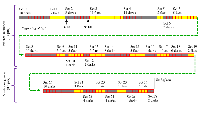
Figure 1: The sequence of flat and dark exposures used in this paper.

5.2 Quantum efficiency, full well, and noise data

Another set of measurements is possible with the quantum efficiency (“qe”), full well (“fw”), and noise (“noise”) data sets taken during acceptance testing. The quantum efficiency data consists of a set of flat fields at many wavelengths, ranging from 480 nm (the shortest science wavelength for the Roman wide field instrument) to beyond the $\sim 2.5$ $\mu$m cutoff of the detectors. This should enable determination of the 2-hole probability as a function of wavelength. However, the quantum efficiency data typically has only 2 flat fields per wavelength and 5 frames per data cube. This means that much more averaging needs to be done with this data than the flat + dark data optimized for correlation function analysis (§5.1). In order to ensure that the results are statistically independent from the flat + dark data, we pair the visible quantum efficiency data with infrared flat fields from the fw data set (at a wavelength of 1.4 $\mu$m) and dark frames from the noise data.

5.3 Simulations

We also generate a simulated suite of data cubes, in which the charge diffusion parameters are known. These can be generated using a modification of the simulation code from Hirata & Choi (2020), which we summarize here. The process begins by reading a user-provided configuration file containing simulation inputs and specifications. Using default settings generates a data cube of size $4096^{2}$ pixels² containing 66 time samples (each having 2 substeps) with the bounding 4 rows and columns designated as reference pixels.

Next, arrays are initialized and charge is drawn from a Poisson distribution and accumulated at each time step. When BFE is turned on, the Poisson distribution is modified at each time step based on pixel area defects. This does not happen in the absence of BFE; each time frame will have a random realization of charge accumulation. Once charge is accumulated over all time frames, it may be optionally convolved with an IPC kernel. If any CNL is desired, it can be applied following the inclusion of IPC. We add a small amount of Gaussian noise to our simulated data. In the final step, we convert charge to data numbers and save the output datacube as a fits file. We direct readers to Figure 1 of Hirata & Choi (2020) to see a flowchart of the simulation procedure.

The principal modification needed to the above process is that in a time step $\delta t$, we need to generate both 1-electron and 2-electron events. Let us first consider what happens without the BFE; in this case, we need to generate some 1-electron events, with a Poisson distribution in each pixel with mean $(1-\omega)I_{\gamma}\delta t$, and some 2-electron events, with a Poisson distribution in each pixel with mean $\omega I_{\gamma}\delta t$. The 1-electron events are straightforward. For the 2-electron events, we write a for loop to run over the possible offsets $(\Delta i,\Delta j)$, and generate 2-electron events with Poisson distribution in each pixel with mean $\omega p_{2}(\Delta i,\Delta j)I_{\gamma}\delta t$. We can add both this array and the same array offset by $(\Delta i,\Delta j)$ to the map of total charge $Q$.

A complication occurs when we include the BFE, since then the pixels have areas that are not identical. Instead of shifting the pixel boundaries in the simulations and following each 2-electron event, we have instead applied the BFE only to the 1-electron events, and increased the magnitude of the pixel area correction by a factor of $1/f$, where $f=(1-\omega)/(1+\omega)$ (since the fraction of electrons coming from 1-electron events is $f$). This is not perfectly realistic, but it captures the correct effective change in area of the pixel, which is the mechanism by which the BFE will appear in the correlation functions.

To ensure realism in our simulations, we base simulation inputs and specifications on real data (or reports) provided by the Detector Characterization Lab (DCL) at NASA’s Goddard Space Flight Center. This includes quantities such as time steps between sampled frames and quantum efficiency. After passing the data through our analysis code, Solid-waffle, we can measure gain, illumination, the linear IPC coefficient, and BFE coefficients. We discuss our simulation inputs and outputs in §6.4.

6 Analysis code

We have expanded the Solid-waffle code to include quantum yield effects. First, the code performs its characterization using the IR flats (+darks) to get the gain $g$, classical non-linearity coefficients $\beta_{j}$, and IPC coefficients $\alpha_{\rm H}$, $\alpha_{\rm V}$, and $\alpha_{\rm D}$, using the same procedure as in Freudenburg et al. (2020). These detector effects operate on already collected charge and should not depend on the wavelength of illumination. We then turn our attention to the visible flats (+darks), which we can use to determine the BFE kernel $[K^{2}a]$ (which could depend on absorption depth and hence wavelength since it acts during the charge collection process), as well as $\omega$ and $p_{2}$ and the current $I_{e}$ used in the visible flats ($I_{e}$ is not a main output of the characterization process, but must be solved in an auxiliary sense).

In what follows, we describe the sequence of steps for the visible flats. The steps are done in each super-pixel, regions of the detector used for analysis over which we measure a correlation function. In most analyses, there are 1024 super-pixels, each composed of $128\times 128$ pixels, but Solid-waffle allows for any power of 2 and for different binnings in the row and column directions if desired.

6.1 Determining $I_{e}$

For each super-pixel, we construct the synthetic correlated double sample images (see Hirata & Choi 2020 for a discussion on their importance) $S_{ad}(x_{1},x_{2}|{\rm F}k)$ for each flat $k$, where $a$ and $d$ are the first and last time slices used for visible characterization. We then take the super-pixel median and subtract the median of the reference pixels for that flat exposure. The default scheme, which we have found to work well on data from the HyC dewar at the DCL, is to use the pixels on the left and right sides; for $128\times 128$ super-pixels, this corresponds to the median of 1024 reference pixels, 512 on each side. We take the mean over the flats to get an averaged signal $\bar{S}_{ad}$ for that super-pixel. This is related to the photocurrent $I_{e}$ by

$$\bar{S}_{ad}=\frac{1}{g}\Bigl{\{}I_{e}t_{ad}-\sum_{j=2}^{p}\beta_{j}[(I_{e}t_{d})^{j}-(I_{e}t_{a})^{j}]\Bigr{\}},$$ (27)

or, with some algebraic rearrangement,

$$I_{e}=\frac{g\bar{S}_{ad}}{t_{ad}-\sum_{j=2}^{p}\beta_{j}I_{e}^{j-1}(t_{d}^{j}-t_{a}^{j})}.$$ (28)

We use this equation iteratively to solve for $I_{e}$ and use a starting guess of $I_{e}=g\bar{S}_{ad}/t_{ad}$ (i.e., without the nonlinearity).

We have experimented with other ways to estimate the current $I_{e}$. The aforementioned method is more robust than methods that used, e.g., the linear coefficient of a polynomial fit, since the latter can suffer from persistence or other effects that are most important in the first couple of frames.

6.2 Measuring the correlation function

We next want to measure a correlation function that contains the information in $\Phi$. If we want to constrain a $5\times 5$ even kernel $\Phi$, then we need a measurement that is also a $5\times 5$ even kernel ${\boldsymbol{v}}$. We choose the same correlation functions that were used in the “Advanced” characterization in Hirata & Choi (2020). That is, we build a $5\times 5$ array ${\boldsymbol{v}}$ of the averaged equal-interval correlation functions of duration $\mu$, built from time slices between $a$ and $d$:

$${\boldsymbol{v}}(\Delta x_{1},\Delta x_{2})=\bar{C}_{a,a+\mu,a,a+\mu,[d-a-\mu]}(\Delta x_{1},\Delta x_{2})=\frac{1}{d-a-\mu}\sum_{k=0}^{d-a-\mu-1}C_{a+k,a+\mu+k,a+k,a+\mu+k}(\Delta x_{1},\Delta x_{2})$$ (29)

for $(\Delta x_{1},\Delta x_{2})\neq(0,0)$. The equal-interval correlation function should be sensitive to the probability of generating pairs of charges in pixels $(x_{1},x_{2})$ and $(x_{1}+\Delta x_{1},x_{2}+\Delta x_{2})$. The averaging reduces noise. For the special case of the correlation function at $(0,0)$, we want to remove the read noise; we thus set

$${\boldsymbol{v}}(0,0)=\Delta V=\bar{C}_{a,a+\mu,a,a+\mu,[d-a-\mu]}(0,0)-\bar{C}_{a,a+\mu^{\prime},a,a+\mu^{\prime},[d-a-\mu^{\prime}]}(0,0),$$ (30)

where $\mu^{\prime}<\mu$ (typically we choose $\mu^{\prime}=1$, $\mu=3$).

6.3 Iteratively solving for quantum yield, charge diffusion, and IPNL parameters

We now enter an iterative loop where $\Phi$ and the IPNL kernel $[K^{2}a]$ are determined. In each iteration, we first update $\Phi$ and then $[K^{2}a]$.

The update to the vector ${\boldsymbol{\Phi}}$ uses an approximate Newton-Raphson iterative step:

$${\boldsymbol{\Phi}}_{n+1}={\boldsymbol{\Phi}}_{n}+{\bf J}^{-1}_{\textrm{approx}}\left[{\boldsymbol{v}}({\rm measured})-{\boldsymbol{v}}({\rm predicted~{}from~{}}{\boldsymbol{\Phi}}_{n})\right].$$ (31)

where ${\boldsymbol{\Phi}}_{n}$ is the “vector” representing the kernel $\Phi$ in the $n$th iteration, and ${\bf J}_{\textrm{approx}}$ is an approximation to the Jacobian $\partial{\bm v}/\partial\Phi$. In this equation, ${\boldsymbol{\Phi}}$ and ${\boldsymbol{v}}$ are understood to be “flattened” length-25 vectors, and the Jacobian is a $25\times 25$ matrix. The predicted ${\boldsymbol{v}}$ is obtained from ftsolve.solve_corr_vis_many (two calls are necessary because of the second term in Eq. 30). The Newton-Raphson method would use the exact Jacobian, but the method converges even with an approximate Jacobian (this saves the time associated with evaluating the Jacobian, but at the expense of requiring more iterations to converge).

We construct our approximate Jacobian as follows. We determine the flat field power spectrum for quantum yield and charge diffusion only (no BFE, IPC, or CNL) by taking the BFE-only case (Eq. 24) and considering the limit when BFE goes to zero:

$$C^{\Phi~{}\rm only}_{abcd}(k_{1}^{\prime}-k_{1},k_{2}^{\prime}-k_{2})=\lim_{\textrm{BFE}\to 0}\widetilde{C}^{\mathrm{BFE}}_{abcd}(k_{1}^{\prime}-k_{1},k_{2}^{\prime}-k_{2})=\frac{I_{e}t_{abcd}N^{2}\delta_{k+k^{\prime},0}}{g^{2}}\left[2\tilde{\Phi}(k_{1}^{\prime},k_{2}^{\prime})+1\right].$$ (32)

(We used l’Hôpital’s rule, and used the overlap $t_{abcd}$ as defined in Hirata & Choi (2020)[Eq. 18].) Data from flats and darks are taken and analyzed in real space, so we Fourier transform Eq. (32), use the fact that $\Phi$ is even, and then find the correlation function

$$C^{\Phi~{}\rm only}_{abcd}(x_{1}-x^{\prime}_{1},x_{2}-x^{\prime}_{2})=\frac{I_{e}t_{abcd}}{g^{2}}\left[2\Phi(x_{1}-x^{\prime}_{1},x_{2}-x^{\prime}_{2})+\delta_{x_{1},x_{1}^{\prime}}\delta_{x_{2},x_{2}^{\prime}}\right].$$ (33)

This suggests that we use the approximate Jacobian

$$J_{\rm approx}(\Delta x_{1},\Delta x_{2};\Delta y_{1},\Delta y_{2})=\frac{\partial v^{\Phi~{}\rm only}(\Delta x_{1},\Delta x_{2})}{\partial\Phi(\Delta y_{1},\Delta y_{2})}=\frac{2I_{e}t_{abcd}}{g^{2}}\delta_{\Delta x_{1},\Delta y_{1}}\delta_{\Delta x_{2},\Delta y_{2}}\times\left\{\begin{array}[]{lll}\mu&&(\Delta x_{1},\Delta x_{2})\neq(0,0)\\ \mu-\mu^{\prime}&&(\Delta x_{1},\Delta x_{2})=(0,0)\end{array}\right..$$ (34)

Because ${\bf J}_{\rm approx}$ is diagonal, the inverse is trivial it can be implemented with element-wise multiplication, rather than explicitly flattening ${\boldsymbol{\Phi}}$ and ${\boldsymbol{v}}$ into vectors, multiplying by a matrix, and turning them back into numpy arrays.

The update of the IPNL kernel $[K^{2}a]$ (here assumed to be mainly BFE) is performed using the same algorithm as in Freudenburg et al. (2020, §4.2.2). The only change necessary to the function that implements this algorithm (pyirc.bfe) is to call the new visible correlation function ftsolve.solve_corr_vis instead of ftsolve.solve_corr, and to put in the piping to ensure that ftsolve.solve_corr_vis has access to the current values of $\omega$ and $p_{2}$.

Once $\Phi(\Delta x_{1},\Delta x_{2})$ is measured, we may solve for the values of $(\omega,C_{11},C_{12},C_{22})$ that minimize the sum of squared residuals assuming a Gaussian charge diffusion model (§3). In the presence of noise, we impose a constraint that ${\bf C}$ be positive definite; in practice, we restrict the minimum eigenvalue of ${\bf C}$ to be $\geq(0.01\,{\rm pix})^{2}$, i.e., the semiminor axis of the charge diffusion must be at least 0.01 pix.

6.4 Tests on simulations

As was done in Hirata & Choi (2020) and Freudenburg et al. (2020), we created a set of simulated flats and darks (both visible and IR) following the procedure outlined in §5.3. All results in this section are from data given in $32\times 32$ bins of superpixels. Figure 2 summarizes the simulation tests. The first row does an analysis for 32$\times$32 superpixels, assumes no IPC, sets input BFE kernels to be different for the IR and visible data (with a stronger impact in the visible data), and a fiducial set of quantum yield and charge diffusion parameters. The second row is similar to the first but with 16$\times$16 superpixels. The third row is similar to the first but with an input IPC. For all three tests, the input gain was $g=1.7285$ e/DN and Solid-waffle returned a consistent output, with the third test giving $g=1.7287\pm 0.0004$ e/DN. We fit the classical nonlinearity curve up to quartic order using polynomial coefficients $\beta_{j}$ (units: electrons^1-j) defined in F/37. We set $\beta_{j}=\{0\}$ and Solid-waffle recovered values of $g\beta_{2},\,g^{2}\beta_{3},\textrm{ and }g^{3}\beta_{4}$ consistent with zero at $1\sigma$. The charge per time slice we passed to the simulation is $3051.5$ e and the output was $2898.9\pm 0.8$ e; this result is consistent with the input quantum efficiency of 95%. We passed IPC components $\alpha_{H}=\alpha_{V}=\alpha=0.01379$ and obtained $\alpha_{H}=0.01367\pm 0.00003,\,\alpha_{V}=0.01363\pm 0.00003$. These correspond to biases of $\sim 1\%$ compared to the inputs. Results discussed thus far are broadly in agreement with those in Freudenburg et al. (2020) which is promising (but unsurprising) since CNL and IPC are unaffected by quantum yield.

For the remainder of this section we review results that depend on quantum yield and charge diffusion parameters. The value of $\omega$ input to Solid-waffle was $0.08$ and it returned $\omega=0.0807\pm 0.0002$. Input values for the charge diffusion covariance matrix were $C_{11}=C_{22}=0.04\textrm{ and }C_{12}=0.02$. Output values were $C_{11}=0.0405\pm 0.0004,\,C_{11}=0.0414\pm 0.0005,\textrm{ and }C_{12}=0.0197\pm 0.0004$.

We now discuss the differences between Solid-waffle simulation inputs and outputs for IPNL. The central pixel IR IPNL kernel returned by Solid-waffle is $[K^{2}a^{\prime}]_{0,0}=-1.8321\pm 0.0058$ (stat) ppm/e, which we compare to the input value $[K^{2}a^{\prime}]_{0,0,\textrm{input}}=-1.7779$ ppm/e. This is a bias of $-0.0542$ ppm/e ($3\%,\,9.3\sigma$) compared to the input value. Solid-waffle gives comparable results for visible simulations. The recovered visible IPNL kernel is $[K^{2}a^{\prime}]_{0,0}=-2.7995\pm 0.0072$ (stat) ppm/e while the input value is $[K^{2}a^{\prime}]_{0,0,\textrm{input}}=-2.6777$ ppm/e. This corresponds to a difference of $-0.1218$ ppm/e ($4.5\%,\,17\sigma$). We also tested our code’s ability to recover the IPNL kernels of symmetrically-averaged nearest neighbor pairs of pixels. We found $[K^{2}a^{\prime}]_{\langle 1,0\rangle}=0.3016\pm 0.0055$ (stat) ppm/e for the IR IPNL kernel. Compared to its input value $[K^{2}a^{\prime}]_{\langle 1,0\rangle,{\rm input}}=0.3001$ ppm/e, this represents a bias of $0.0015$ ppm/e ($0.50\%,\,0.28\sigma$). Similarly, in the visible case we recovered $[K^{2}a^{\prime}]_{\langle 1,0\rangle}=0.3148\pm 0.0036$ (stat) ppm/e which can be compared to the given value $[K^{2}a^{\prime}]_{\langle 1,0\rangle,{\rm input}}=0.3033$ ppm/e. This translates to a bias of $0.0115$ ppm/e ($3.8\%,\,3.2\sigma$). We do not find significant differences in results when using $16\times 16$ bins of superpixels.

For the IR case we can directly compare the above IPNL kernel results to those in Freudenburg et al. (2020). Therein, the authors found a $0.96\%$ bias between inputs and outputs for the central pixel and a bias of $1.5\%$ for the symmetrically-averaged nearest neighbors. Those percentages are similar to what we find in this work, 3% for central pixel and 0.5% for nearest neighbors.

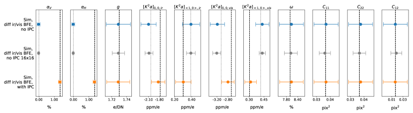
Figure 2: Simulation tests. Each row corresponds to a simulation variation. The vertical lines indicate input simulation values. For the panels that have two dashed vertical lines, the long-dashed line indicates the input values corresponding to simulation variations with non-zero IPC.

7 Results for Roman detector arrays

We now apply our updated formalism to Roman flight candidates SCAs 20663, 20828, and 20829. Details of the fiducial set of visible detector runs we use in this paper are given in Tables 2 – 5. Following Freudenburg et al. (2020), some results will only be provided for SCA 20829 for brevity. In the future we expect to set up a public repository where other results will be made available.

7.1 Superpixel maps for SCA 20829

Figure 3 shows the spatial distributions of derived IR characterization quantities across SCA 20829, and Figure 4 does the same for derived visible quantities. Figure 3 is very similar to Figure 8 of Freudenburg et al. (2020), which is expected because there are no changes to this part of the measurement and relatively minor changes to the set-up (time frames used for the correlation analysis and non-linearity curve fitting and different input flats and darks). A few important points should be noted about these data. First, the illumination pattern, while smooth, is not exactly flat, so the gradient in charge per frame ($It_{n,n+1}$) is not necessarily a property of the SCA. Second, the probability $\omega$ of generating two electron-hole pairs is highest in the upper left corner of the detector. We have not identified the cause of this behavior, and it is not seen in the other SCAs. Last, the $C_{11}$ and $C_{22}$ components of the charge diffusion covariance matrix are the same to within 10%. This is convenient for weak lensing applications, since $C_{11}-C_{22}$ is a source of ellipticity ($e_{1}$ component). It is expected behavior since the electric field structure in the HgCdTe layer should not distinguish the $x$ vs. $y$ axes. This can be contrasted with CCDs, where there is a readout direction and there are generally higher potential barriers between adjacent columns than between adjacent rows.

Figure 3: Detector maps showing the spatial variation of IR characterization parameters for SCA 20829. This is binned into 1024 superpixels each composed of $128\times 128$ pixels. These maps agree with their counterparts (when present) in Freudenburg et al. (2020). $\beta$ shown in the center right map is $\beta_{2}$ from Equation 35. The nonlinearity polynomial coefficients $\beta_{j}$ are strongly anticorrelated (correlation coefficient $-0.94$ between $\beta_{2}$ and $\beta_{3}$, and $-0.96$ between $\beta_{3}$ and $\beta_{4}$), so large variations seen in $\beta_{2}$ correspond to smaller variations in the total nonlinearity.

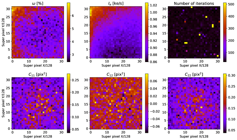
Figure 4: Detector maps showing the spatial variation of visible characterization parameters for SCA 20829. This is binned into 1024 superpixels each composed of $128\times 128$ pixels. Number of iterations refers to the number of steps required for the $\Phi$ kernel to converge (see §6.3).

7.2 Recovering detector parameters

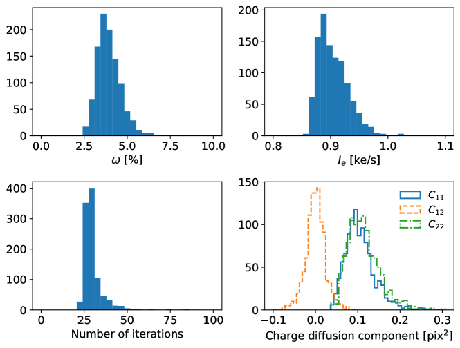
Figure 5: Histograms of visible characterization results for SCA 20829. The $y$-axis counts the number of superpixels falling into each bin. Number of iterations refers to the number of steps required for the $\Phi$ kernel to converge.

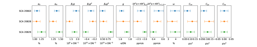
Figure 6: Fiducial characterization results for each SCA averaged over all superpixels (see Table 1 for the numerical values for each SCA). Note that the IPNL values shown are for the visible case, although the ‘vis’ tag has been omitted here for readability.

Mean values and standard deviations on the mean (both taken across all superpixels) for infrared IPNL, visible IPNL, and IPC parameters are given in Table 1 for the three flight candidates. Figure 5 offers a visual representation of quantum yield and charge diffusion properties for SCA 20829, while Figure 6 summarizes most data from Table 1 as a whisker plot.

First, we compare IR characterization results from our analyses to those reported in the fidicual results of Freudenburg et al. (2020). Values of charge per time slice, gain, and all four IPC $\alpha$ parameters are consistent at the $<1\sigma$ level for all detectors. The large-scale variation in gain across SCA 20829, as shown in the upper right of Figure 3, is consistent between the two works, and similar variations are seen in other Roman flight candidates at the DCL. The CNL parameters $\beta_{j}g^{1-j}$ between the two works are significantly different for all detectors, with differences ranging from $4.0-9.3\sigma$ for 20663, $3.3-8.2\sigma$ for 20828, and $5.6-16.2\sigma$ for 20829, and increasing as $j$ increases. However, the nonlinearity curves were fit over different time ranges for the two papers, which could understandably lead to the large differences in the fitted $\beta_{j}$. Thus, it may be more instructive to compare the mapping between charge and signal following F/32 which gives

$$S_{a}=\frac{1}{g}\left[\bar{Q}(t_{a})-\beta_{2}\bar{Q}(t_{a})^{2}-\beta_{3}\bar{Q}(t_{a})^{3}-\beta_{4}Q(t_{a})^{4}\right].$$ (35)

At time frame 10, $S_{10}=18765.19\pm 17.13$ (Freudenburg et al., 2020) and $S_{10}=18754.38\pm 23.63$ (this work), where errors are obtained by propagating the standard errors from the charge per time slice, gain, and nonlinearity parameters. These signal values are entirely consistent. Finally, neighboring pixel IPNL kernel results for each detector are consistent with those reported in Freudenburg et al. (2020) at $\lesssim 1\sigma$. However, the central pixel results are discrepant at $\sim 2\sigma$ in each case. The discrepancy may be a result of this work and Freudenburg et al. (2020) using different sequences of flats and darks as well as different time slices.

We now compare visible characterization results between detectors and compare IR and visible IPNL kernels for each detector. SCA 20663 has the greatest current per pixel of the flight candidates, beating out SCA 20828 by a factor of 1.45 and SCA 20829 by a factor of 1.53. We suspect that this is due to differences in light source intensity hitting each detector. All three detectors show evidence of $\omega>0$ at the $5-6\sigma$ level for each superpixel. For every photon absorbed by these detectors, more than 1.035 charge carriers are collected on average. The charge diffusion variance contributions $C_{11}$ and $C_{22}$ are detected at $3\sigma$ for each SCA while the covariance term ($C_{12}$, describing whether there is more diffusion in the northeast-southwest direction than the northwest-southeast direction on the SCA) is consistent with zero. We have also shown the charge diffusion length, which we have given as the $1\sigma$ scale of a 2-dimensional Gaussian:

$$\sigma_{\rm cd}=(10\,\mu{\rm m})\times\sqrt{\frac{C_{11}+C_{22}}{2}}.$$ (36)

Here the factor of 10 $\mu$m converts from pixel units to physical length. The array average charge diffusion lengths reported are 2.7, 3.5, and 3.3 $\mu$m for SCAs 20663, 20828, and 20829, respectively.

In all three detectors we see that the visible central pixel IPNL kernel has a larger absolute value than its IR counterpart, but this difference is consistent with zero after considering the standard deviation. The rate of decline in the absolute value of the IPNL kernel as one goes from $(0,0)$ to $\langle 1,0\rangle$ to $\langle 2,0\rangle$ is approximately the same for IR and visible characterizations.

		SCA 20663		SCA 20828		SCA 20829
Quantity	Units	fid	$\sigma({\rm fid})$	fid	$\sigma({\rm fid})$	fid	$\sigma({\rm fid})$
IR characterization
Charge, $It_{n,n+1}$	ke	3.4918	0.0433	3.0816	0.0319	3.0376	0.0333
Gain $g$	e/DN	1.6264	0.0444	1.6696	0.0618	1.7357	0.0420
IPC $\alpha$	%	1.2234	0.0743	1.1508	0.1085	1.3520	0.1077
IPC $\alpha_{\rm H}$	%	1.3624	0.0808	1.2363	0.1185	1.4483	0.1068
IPC $\alpha_{\rm V}$	%	1.0844	0.0991	1.0653	0.1420	1.2556	0.1508
IPC $\alpha_{\rm D}$	%	0.1231	0.0478	0.1215	0.0463	0.1407	0.0423
$\beta_{2}g$	$10^{6}\times$DN-1	1.8884	0.2270	1.3793	0.2391	1.7637	0.1889
$\beta_{3}g^{2}$	$10^{10}\times$DN-2	$-$0.2857	0.0780	$-$0.2354	0.0840	$-$0.4255	0.0662
$\beta_{4}g^{3}$	$10^{15}\times$DN-3	0.4966	0.1109	0.5329	0.1471	0.8553	0.0895
$[K^{2}a+KK^{I}]_{0,0\textrm{, IR}}$	ppm/e	$-$2.2839	0.2823	$-$2.5582	0.3050	$-$1.9714	0.1422
$[K^{2}a+KK^{I}]_{\langle 1,0\rangle\textrm{, IR}}$	ppm/e	0.5091	0.0975	0.4800	0.0769	0.3946	0.0596
$[K^{2}a+KK^{I}]_{\langle 1,1\rangle\textrm{, IR}}$	ppm/e	0.1626	0.0871	0.1351	0.0676	0.1117	0.0610
$[K^{2}a+KK^{I}]_{\langle 2,0\rangle\textrm{, IR}}$	ppm/e	0.0561	0.0813	0.0219	0.0607	0.0303	0.0608
$[K^{2}a+KK^{I}]_{\langle 2,1\rangle\textrm{, IR}}$	ppm/e	0.0358	0.0651	0.0098	0.0445	0.0151	0.0447
$[K^{2}a+KK^{I}]_{\langle 2,2\rangle\textrm{, IR}}$	ppm/e	0.0254	0.0701	0.0022	0.0657	0.0055	0.0632
$[K^{2}a+KK^{I}]_{\rm H\textrm{, IR}}$	ppm/e	0.4996	0.1182	0.4644	0.1003	0.3742	0.0858
$[K^{2}a+KK^{I}]_{\rm V\textrm{, IR}}$	ppm/e	0.5186	0.1072	0.4957	0.0995	0.4150	0.0813
Visible characterization
$I_{e}$	ke/s	1.3821	0.0286	0.9522	0.0251	0.9048	0.0264
$\omega$	%	3.8939	0.6118	3.5296	0.6568	3.9290	0.6646
$C_{11}$	pix2	0.0745	0.0293	0.1212	0.0441	0.1066	0.0364
$C_{12}$	pix2	0.0001	0.0275	0.0000	0.0245	0.0001	0.0227
$C_{22}$	pix2	0.0754	0.0293	0.1299	0.0479	0.1136	0.0376
$\sigma_{\rm cd}$	$\mu$m	2.7061	0.4121	3.5180	0.4878	3.2890	0.4341
$[K^{2}a+KK^{I}]_{0,0\textrm{, vis}}$	ppm/e	$-$2.6909	0.5960	$-$2.6048	0.3426	$-$2.0872	0.1780
$[K^{2}a+KK^{I}]_{\langle 1,0\rangle\textrm{, vis}}$	ppm/e	0.5844	0.0860	0.4713	0.0953	0.3765	0.0808
$[K^{2}a+KK^{I}]_{\langle 1,1\rangle\textrm{, vis}}$	ppm/e	0.1517	0.0757	0.1312	0.0903	0.1044	0.0847
$[K^{2}a+KK^{I}]_{\langle 2,0\rangle\textrm{, vis}}$	ppm/e	0.0252	0.0713	0.0221	0.0875	0.0188	0.0830
$[K^{2}a+KK^{I}]_{\langle 2,1\rangle\textrm{, vis}}$	ppm/e	0.0077	0.0516	0.0131	0.0599	0.0074	0.0594
$[K^{2}a+KK^{I}]_{\langle 2,2\rangle\textrm{, vis}}$	ppm/e	0.0011	0.0762	-0.0028	0.0874	0.0007	0.0847
$[K^{2}a+KK^{I}]_{\rm H\textrm{, vis}}$	ppm/e	0.5669	0.1135	0.4509	0.1286	0.3521	0.1151
$[K^{2}a+KK^{I}]_{\rm V\textrm{, vis}}$	ppm/e	0.6018	0.1152	0.4918	0.1237	0.4009	0.1148

Table 1: Characterization results for SCAs 20663, 20828, and 20829 averaged over all superpixels. Rows refer to the fiducial configuration as described in Table 5. Subscripts H and V on the IPNL kernel indicate the average of the horizontal and vertical nearest neighbors to the central pixel. Subscripts in angled brackets indicate averages over nearest neighbors, averages over diagonal neighbors, etc. For each SCA, the first column lists the value of that quantity in the fiducial run, and the second column lists the standard deviation of the superpixels for each quantity. The top portion of this table comes from IR characterization while the bottom portion comes from visible characterization.

7.3 Quantum yield vs. wavelength

The quantum efficiency dataset (“qe”) can be used to measure the quantum yield as a function of wavelength. Several modifications to the configuration were needed to achieve this. First, since there are only 2 flats at each wavelength, we made larger super-pixels, each consisting of $128\times 512$ pixels (so that there are 256 super-pixels total, each one readout channel wide, and with 8 super-pixels along the vertical direction in each channel). Second, since there are only 5 time stamps and the signal level is sometimes low, the qe data do not constrain the BFE kernel; we used the Solid-waffle keyword COPYIRBFE, which sets the visible kernel $[K^{2}a]$ equal to that obtained from the IR flats rather than fitting it from the correlation function of the visible data. Finally, the fitting of the covariance matrix and quantum yield parameter from the $\Phi$ kernel is unstable when $\omega$ is small and the signal:noise ratio is low; therefore, we have estimated the 2-hole probability from

$$\omega(\lambda)=\frac{\sum_{\Delta x_{1},\Delta x_{2}}\Phi(\Delta x_{1},\Delta x_{2})}{1-\sum_{\Delta x_{1},\Delta x_{2}}\Phi(\Delta x_{1},\Delta x_{2})}.$$ (37)

(this is Eq. 3, summed using the normalization $\sum p_{2}=1$, and after solving for $\omega$). This form is numerically stable even if $\omega$ fluctuates to a negative value. We report both the median of $\omega$ over all 256 super-pixels, and the standard error on the median.

Results are shown in Fig. 7 for all 3 SCAs. The probability of collecting 2 holes rises as a function of photon energy; we observe a threshold at $\lambda^{-1}\approx 1.2\,\mu$m^-1 ($\lambda\approx 830$ nm), where the photon has approximately 3 times the band gap energy. This is similar to behavior observed for other devices (see, e.g., Table 2 of Rauscher et al. 2014). Interestingly, at 500 nm or 0.6 eV above threshold, the probability of collecting 2 holes is only $\sim 4\%$, which is much less than what we would expect from studies of other semiconductors such as Si, Ge, or 5 $\mu$m cutoff HgCdTe (Rauscher et al., 2014, Fig. 7) — the JWST NIRSpec detectors, for example, show a $\sim 30\%$ probability at $E-E_{\rm t}=0.6$ eV. Regardless of the microphysical cause, the low probability of collecting 2 holes reduces the signal:noise ratio of the charge diffusion measurement. Another unexpected behavior that we observe is a peak at $\lambda^{-1}\sim 1.8\,\mu$m^-1 ($\lambda\approx 560$ nm), followed by a decline as we go to the blue. Note that there is good agreement with our analysis of the flats + darks in §7.2 at 500 nm. We discuss possible explanations for the declining quantum yield in §8.

The 2-hole probabilities in Fig. 7 show an offset from zero at small wavenumber (where generation of a second electron-hole pair is not energetically possible). This offset ranges from 0.15% for SCA 20663 to 0.47% for SCA 20828; such an offset could arise if there were a systematic difference in gain between the quantum efficiency and full well flat fields. It is worth noting that the full well data reaches saturation, and that of the three detector arrays studied here, SCA 20663 had the lowest persistence and burn-in and SCA 20828 had the highest (Freudenburg et al., 2020). We suspect that burn-in effects in the infrared flat field data (the full well data) may be affecting the gain determination and contributing to the offset. We expect we could reduce this problem by acquiring additional flat field data that cover the required range of signal level, but does not approach saturation.

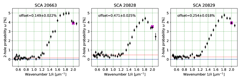
Figure 7: The dependence of the probability $\omega$ of producing 2 holes as a function of wavelength. The black points with error bars are the results from the qe data set. The magenta X denotes the results from Table 1 from the 500 nm flats ($\lambda^{-1}=2.0\,\mu$m^-1). The probability peaks at $\lambda^{-1}\sim 1.8\,\mu$m^-1 and declines again toward bluer wavelengths. The probability $\omega$ should go to zero at redder wavelengths; we find an offset (reported in the caption) that is likely due to systematic errors (see main text).

7.4 Impact of charge diffusion on the shear signal

To estimate the impact of charge diffusion on the weak lensing shear signal, we take a fiducial set of visible detector runs — whose details are outlined in Table 5 — and measure their respective charge diffusion covariance matrices (see §3) in $32\times 32$ bins of superpixels. We visualize the covariance matrix in each superpixel using publicly available code which prints an ellipse associated with each covariance. This is shown for SCA 20829 in Figure 8. Given an ellipticity field for each detector (and the fact that this work is a weak lensing analysis), it is natural for us to consider converting these shapes into a set of shears just as one would do for a galaxy ellipticity field on a patch of sky.

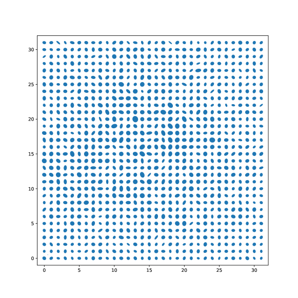
Figure 8: Elliptical grid based on charge diffusion covariance matrices for SCA 20829. The radius of each ellipse is set to two standard deviations. The vertical and horizontal axes label superpixel indices.

The conversion from components of charge diffusion covariance to shear can be obtained using the methodology in Troxel et al. (2021). There the aim was to estimate the effect of image motion on the galaxy ellipticity and hence the shear, but since both image motion and charge diffusion convolve the point spread function (PSF) with a kernel — either the probability density function of the image motion in that case or $P_{\rm cd}({\boldsymbol{\xi}})$ here — the results from Troxel et al. (2021) can be carried over to our case. In the worst-affected redshift bin, the shear error induced by charge diffusion is

$$\gamma_{1}=K_{\theta\theta}(C_{11}-C_{22}),$$ (38)

$$\gamma_{2}=2K_{\theta\theta}C_{12},$$

where $K_{\theta\theta}=1.432\times 10^{-5}\textrm{~{}mas}^{-2}=0.1733\textrm{~{}pix}^{-2}$ (Troxel et al., 2021, Table B1). Next we pass a list of superpixel indices (converted to arcsec) and shears to TreeCorr (Jarvis et al., 2004) which calculates the shear correlation functions $\xi_{+}(\theta)$ and $\xi_{-}(\theta)$. Results for the three SCAs are shown in Figure 9.

Roman requirements on additive shear variance per component in each bin of multipole $\ell$ are given in its Science Requirements Document. A single detector has maximum and minimum separations corresponding to harmonic scales $10^{3}<\ell<10^{3.5}$ ($0.001<\theta\textrm{ (rads)}<0.0031$) which lies in the highest $\ell$ bin. We compare the charge diffusion “shear” to Roman requirements using three different approaches, one in configuration space and two in harmonic space. This is done as a consistency check since each approach uses different approximations; once all 18 flight detectors are selected and their layout in the focal plane is chosen, it will be possible to tile the sky and unambiguously predict the spurious shear due to charge diffusion for a given tiling strategy.

In the first approach, we start with the equation

$$\xi_{+}(\theta)=\int_{0}^{\infty}\frac{\ell d\ell}{2\pi}J_{0}(\ell\theta)[C_{EE}(\ell)+C_{BB}(\ell)]\simeq\sum_{\ell\textrm{ bins}}2\gamma^{2}\overline{J_{0}(\ell\theta)},$$ (39)

where $J_{0}$ is the Bessel function, $C(\ell)$ is the shear power spectrum (with the subscript ’EE’ or ’BB’ referring to the E-mode and B-mode power spectra components, respectively), $\gamma$ is the component of shear, and the overline indicates the average value over $\ell$. In the $\ell$ bin of interest, $\gamma=1.9\times 10^{-4}$ and we make the rough estimate $\overline{J_{0}(\ell\theta)}\sim\mathcal{O}(10^{-1})$ for ease of calculation. The ratio of the measured charge diffusion correlation function to our estimate of Roman requirements is $\xi_{+,\textrm{ Fig.9}}/\xi_{+,\textrm{ Eq.36}}\sim 20$ over smaller separations in the detector.

In the second approach, we take the $\xi_{+}$ correlation function measured by TreeCorr and Hankel transform it using the hankel Python library (Murray & Poulin, 2019) to get $C_{EE}(\ell)+C_{BB}(\ell)$. The variance per component over the $\ell$ bin for SCA 20829 is

$$\textrm{var per comp}=\int_{10^{3}}^{10^{3.5}}\frac{d\ell}{4\pi}\ell[C_{EE}(\ell)+C_{BB}(\ell)]=-2.2\times 10^{-6}.$$ (40)

This is $|\textrm{var per comp}/\gamma^{2}|\sim 60$ greater than requirements.

For the final comparison, we obtain theory predictions for $\xi_{+}$ from the publicly available theory pipeline CosmoSIS (Zuntz et al., 2015), artificially tweaking $\sigma_{8}$ to get theory predictions that roughly agree with the measured values of $\xi_{+}$ values for each detector. CosmoSIS gives the associated $C_{\ell}$’s which we plug into Eq. (40). The variance per component calculated this way is $4.5\times 10^{-7}$, which is a factor of $\sim 12$ above requirements.

The above results show factors of systematic error in power which are all $\mathcal{O}(10)$. Weak lensing systematics mitigation through point spread function fitting acts on amplitudes. This means that systematic errors on shear need to be reduced by $\mathcal{O}(1)$ (i.e., the square root of the systematic error in power) which is doable using standard techniques. Charge diffusion affects images of stars as well, so if it were perfectly linear (i.e., the covariance matrix of the charge diffusion is independent of the amount of charge already in the well), then it would be absorbed as part of PSF fitting. Next-order effects, such as wavelength and signal dependence of charge diffusion, could be expected since the conversion depth depends on the wavelength of illumination and the previously accumulated signal changes the electric field geometry (as evidenced by the BFE). The strength of these effects will determine how much complexity is needed in modeling and mitigating the systematics from charge diffusion.

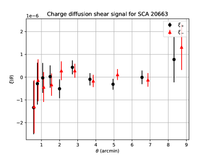
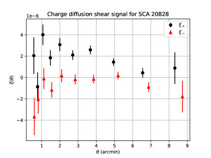
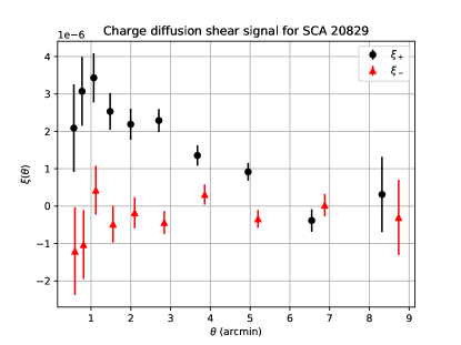
Figure 9: Top panel: Charge diffusion correlation functions $\xi_{+}(\theta)$ (black circles) and $\xi_{-}(\theta)$ (red triangles) measured on SCA 20663 data by TreeCorr. A 5% offset in $\theta$ was added to the plot of $\xi_{-}$ for ease of visualization. Middle panel: Same for SCA 20282 (the three super pixels where Solid-waffle failed to converge are masked). Bottom panel: Same for SCA 20829.

8 Discussion

This paper has presented a formalism for the inclusion of quantum yield and charge diffusion effects in Fourier-space correlations of HxRG detector array visible flat and dark fields, expanding on the work of Freudenburg et al. (2020) which considered only IR flat and dark field correlations. We updated Solid-waffle to incorporate these changes and return measurements of visible characterization parameters in addition to the IR characterization parameters it previously output. We tested this updated machinery on simulations, finding we could recover IR and visible IPNL kernel parameters to within a few percent.

We have also run our updated analyses on Roman flight candidate detectors SCAs 20663, 20828, and 20829 and presented the detailed results in §7. For the fiducial set of configuration parameters, SCA 20663 had the largest values for the visible IPNL kernel. This is in contrast to the IR case where SCA 20828 holds this distinction. In all three detectors, both IR and visible IPNL kernel values are seen to be slightly asymmetric between rows and columns. For example, $([K^{2}a+KK^{I}]_{\rm H}-[K^{2}a+KK^{I}]_{\rm V})/([K^{2}a+KK^{I}]_{\rm H}+[K^{2}a+KK^{I}]_{\rm V})=-0.052\pm 0.005$ (SCA 20829 IR) and $([K^{2}a+KK^{I}]_{\rm H}-[K^{2}a+KK^{I}]_{\rm V})/([K^{2}a+KK^{I}]_{\rm H}+[K^{2}a+KK^{I}]_{\rm V})=-0.065\pm 0.007$ (SCA 20829 vis). The asymmetry for the IR and visible data are fairly consistent at $\sim 1.5\sigma$.

All detectors showed statistically significant amounts of quantum yield and charge diffusion at 500 nm. The quantum yield measured in each SCA begins to increase at $\lambda^{-1}>1.2\,\mu$m^-1, which is similar to what we would expect scaling from 5 $\mu$m cutoff H2RGs (Rauscher et al., 2014). This is expected behavior since in both cases a minimum energy is needed to produce the second electron-hole pair. However, at 500 nm, the quantum yield measured in this paper ($\omega\sim 3.5-3.9\%$) is smaller than the fits obtained by Rauscher et al. (2014); their fit implies a quantum yield (our $1+\omega$) of 1.65 at 600 nm and 1.27 at 1 $\mu$m (photon energy of $5\times$ the band gap energy, as for Roman detectors at 500 nm). We do not necessarily expect the production of the second electron-hole pair to simply scale with the band gap, however, since most of the band structure does not simply scale.

Another possible explanation is that a significant fraction of the photons are getting absorbed in the buffer layer, as shown in Mosby et al. (2020, Fig. 3), where the band gap is wider and the probability of a second electron-hole pair is less than in a $2.5\,\mu$m band gap material. Our results from §7.3, in which the quantum yield peaks at $\sim 560$ nm and then declines at shorter wavelengths, also seem plausible in this picture, since the mean free path is very short at those wavelengths (see Djurišić & Li, 1999, Fig. 7).

The charge diffusion $\sigma_{\rm cd}$ of 2.7–3.5 $\mu$m measured in this paper is larger than the prediction of 2.04 $\mu$m from the random walk model Mosby et al. (2020, Eq. 22). It is possible that the numerical pre-factor of $1/\pi$ in the Mosby et al. (2020) may be modified with a full treatment of the drift-diffusion problem (with, for example, a distribution of drift times), or that some of the input parameters are slightly different from the as-built values. More interestingly, Mosby et al. (2020) note that their $\sigma_{\rm cd}=2.0\,\mu$m prediction is consistent with ⁵⁵Fe X-ray events (in which there is an additional cross-talk to the nearest neighbor pixels beyond the IPC measured from the single pixel reset method). One potential source of this difference is where the X-rays are absorbed relative to the 500 nm visible photons. The X-rays produced by the ⁵⁵Fe source are predominately Mn KL₂+KL₃ X-rays with energy 5.89 keV (Deslattes et al., 2003, 2005), which in Hg_1-xCd_xTe with $x=0.445$ have an opacity of 523 cm²/g (Berger et al., 2010); at the absorber density of $\rho=7.07$ g/cm³ (Capper, 1994), this corresponds to an absorption depth of $(\kappa\rho)^{-1}=2.7\,\mu$m, or about half of the thickness of the Hg_1-xCd_xTe absorber. In contrast, the absorption depth of a photon at 500 nm in Hg_1-xCd_xTe is 28 nm (Djurišić & Li 1999; in practice, such a photon may be absorbed in the buffer layer). We thus anticipate that holes released by X-ray absorption events likely travel only part way through the absorbing layer, and thus on average may give a lower charge diffusion length than a measurement with visible light.

This work made the first estimate of how much the measured charge diffusion should affect the weak lensing shear signal. For all detectors, we find the charge diffusion shear correlation function $\xi_{+}\sim 10^{-6}$ which is about 1% of the galaxy shear correlation function. We compared the measured charge diffusion $\xi_{+}$ (and $C_{\ell}$) for SCA 20829 to Roman requirements on additive shear per component in the highest $\ell$ bin and found measured values that are $\mathcal{O}(10)$ larger. A more detailed analysis of this effect will be carried out once the layout of all 18 detectors across the Roman focal plane is chosen. Note that this impact is described without taking into account any PSF mitigation. The standard approach taken in weak lensing analyses is to determine a PSF based on stars and interpolate between star positions on the focal plane (for a review, see Section 2.1 of Mandelbaum, 2018). In the case where the density of stars is not enough for direct interpolation (e.g., with a polynomial fit) to capture PSF variations on the smallest spatial scales, principal component methods can be applied to use all available data to identify the most important dimensions of PSF variance (Jarvis & Jain, 2004) and have been shown to be effective on space-based data from the Hubble Space Telescope Advanced Camera for Surveys (Jee et al., 2007; Schrabback et al., 2010). A potential choice to investigate in future work would be to include the 500 nm charge diffusion map or a similar map from the in-flight $r$-band flat fields as an additional basis mode to constrain the PSF fit.

This analysis is one of many that are required to calibrate effects present in Roman detectors. Such calibration will be necessary for the accurate determination of scientific results, including cosmological parameter estimates, from Roman pipelines once the survey begins collecting data. We have extended the correlation function formalism of Freudenburg et al. (2020) to account for quantum yield and charge diffusion effects in the presence of visible light. We applied this updated formalism to three Roman flight candidates — SCAs 20663, 20828, and 20829 — and measured over a dozen new parameters. Just as we did in our previous investigation (Freudenburg et al., 2020), we caution readers that all data were taken under laboratory conditions and that there will likely be some differences with Roman observations, most notably the flight controller (ACADIA, Loose et al. 2018) instead of the Leach controller. In future work we will carry out the same analyses done in this paper on other flight candidates, and with data acquired with the flight SCAs connected to an ACADIA controller. We also plan to compare the charge diffusion measurements obtained via the visible flat field method to measurements obtained with spot projection (Seshadri et al. 2013; a similar test is planned for one of the Roman development detectors). The two methods are expected to have complementary strengths: the visible flat field method provides true averages over regions on the array, and only corresponds to diffusion of charge without the optical PSF or image motion; on the other hand, the spot projection is more similar to what happens when one observes a PSF star, and can be used over the full range of wavelengths including in the NIR where multiple electron-hole pair production does not occur.

Software: Astropy (Astropy Collaboration et al., 2013, 2018), fitsio (Sheldon, 2019), Matplotlib (Hunter, 2007), NumPy (Oliphant, 2006–), SciPy (Virtanen et al., 2020)

Appendix A Frames and configuration file passed to Solid-waffle

Here we provide the sequence of frames (including their full location within the Ohio Supercomputer Center) passed to Solid-waffle via a configuration file for each detector. These frames are paired with the settings given in Table 5. Tables 2, 3, and 4 correspond to SCAs 20663, 20828, and 20829, respectively. These frames are paired with the settings given in Table 5.

LIGHT:

$\sim$/SCA20663/20190926_95K_1p1m0p1_ch1_1400nm_gr3_filt5_shutter_open_20663_001.fits

⋮  (increment last value by 001)

$\sim$/SCA20663/20190926_95K_1p1m0p1_ch1_1400nm_gr3_filt5_shutter_open_20663_005.fits

$\sim$/SCA20663/20190926_95K_1p1m0p1_ch3_1400nm_gr3_filt5_shutter_open_20663_001.fits

⋮  (increment last value by 001)

$\sim$/SCA20663/20190926_95K_1p1m0p1_ch3_1400nm_gr3_filt5_shutter_open_20663_011.fits

DARK:

$\sim$/SCA20663/20190926_95K_1p1m0p1_ch0_1400nm_gr3_filt5_shutter_closed_20663_001.fits

⋮  (increment last value by 001)

$\sim$/SCA20663/20190926_95K_1p1m0p1_ch0_1400nm_gr3_filt5_shutter_closed_20663_010.fits

$\sim$/SCA20663/20190926_95K_1p1m0p1_ch2_1400nm_gr3_filt5_shutter_closed_20663_002.fits

⋮  (increment last value by 001)

$\sim$/SCA20663/20190926_95K_1p1m0p1_ch2_1400nm_gr3_filt5_shutter_closed_20663_007.fits

VISLIGHT:

$\sim$/SCA20663/20190926_95K_1p1m0p1_ch21_500nm_gr3_filt6_shutter_open_20663_001.fits

$\sim$/SCA20663/20190926_95K_1p1m0p1_ch23_500nm_gr3_filt6_shutter_open_20663_001.fits

$\sim$/SCA20663/20190926_95K_1p1m0p1_ch25_500nm_gr3_filt6_shutter_open_20663_001.fits

⋮  (repeat the set of three lines above twice, once ending with 002 and once with 003)

VISDARK:

$\sim$/SCA20663/20190926_95K_1p1m0p1_ch20_500nm_gr3_filt6_shutter_closed_20663_002.fits

⋮  (increment last value by 001)

$\sim$/SCA20663/20190926_95K_1p1m0p1_ch20_500nm_gr3_filt6_shutter_closed_20663_010.fits

Table 2: Frames passed to configuration file for the fiducial set up of SCA 20663.

LIGHT:

$\sim$/SCA20828/20191204_95K_1p1m0p1_ch1_1400nm_gr3_filt5_shutter_open_20828_001.fits

⋮  (increment ch values by 2, i.e. go to the next odd value)

$\sim$/SCA20828/20191204_95K_1p1m0p1_ch17_1400nm_gr3_filt5_shutter_open_20828_001.fits

$\sim$/SCA20828/20191204_95K_1p1m0p1_ch1_1400nm_gr3_filt5_shutter_open_20828_002.fits

⋮  (increment ch values by 2, i.e. go to the next odd value)

$\sim$/SCA20828/20191204_95K_1p1m0p1_ch13_1400nm_gr3_filt5_shutter_open_20828_002.fits

DARK:

$\sim$/SCA20828/20191204_95K_1p1m0p1_ch0_1400nm_gr3_filt5_shutter_closed_20828_001.fits

⋮  (increment last value by 001)

$\sim$/SCA20828/20191204_95K_1p1m0p1_ch0_1400nm_gr3_filt5_shutter_closed_20828_009.fits

$\sim$/SCA20828/20191204_95K_1p1m0p1_ch2_1400nm_gr3_filt5_shutter_closed_20828_002.fits

⋮  (increment last value by 001)

$\sim$/SCA20828/20191204_95K_1p1m0p1_ch2_1400nm_gr3_filt5_shutter_closed_20828_008.fits

VISLIGHT:

$\sim$/SCA20828/20191204_95K_1p1m0p1_ch21_500nm_gr3_filt6_shutter_open_20828_001.fits

$\sim$/SCA20828/20191204_95K_1p1m0p1_ch23_500nm_gr3_filt6_shutter_open_20828_001.fits

$\sim$/SCA20828/20191204_95K_1p1m0p1_ch25_500nm_gr3_filt6_shutter_open_20828_001.fits

⋮  (repeat the set of three lines above twice, once ending with 002 and once with 003)

VISDARK:

$\sim$/SCA20828/20191204_95K_1p1m0p1_ch20_500nm_gr3_filt6_shutter_closed_20828_002.fits

⋮  (increment last value by 001)

$\sim$/SCA20828/20191204_95K_1p1m0p1_ch20_500nm_gr3_filt6_shutter_closed_20828_010.fits

Table 3: Frames passed to configuration file for the fiducial set up of SCA 20828.

LIGHT:

$\sim$/SCA20829/20191018_95K_1p1m0p1_ch1_1400nm_gr3_filt5_shutter_open_20829_001.fits

⋮  (increment ch values by 2, i.e. go to the next odd value)

$\sim$/SCA20829/20191018_95K_1p1m0p1_ch17_1400nm_gr3_filt5_shutter_open_20829_001.fits

$\sim$/SCA20829/20191018_95K_1p1m0p1_ch1_1400nm_gr3_filt5_shutter_open_20829_002.fits

⋮  (increment ch values by 2, i.e. go to the next odd value)

$\sim$/SCA20829/20191018_95K_1p1m0p1_ch13_1400nm_gr3_filt5_shutter_open_20829_002.fits

DARK:

$\sim$/SCA20829/20191018_95K_1p1m0p1_ch0_1400nm_gr3_filt5_shutter_open_20829_001.fits

⋮  (increment last value by 001)

$\sim$/SCA20829/20191018_95K_1p1m0p1_ch0_1400nm_gr3_filt5_shutter_open_20829_009.fits

$\sim$/SCA20829/20191018_95K_1p1m0p1_ch2_1400nm_gr3_filt5_shutter_open_20829_002.fits

⋮  (increment last value by 001)

$\sim$/SCA20829/20191018_95K_1p1m0p1_ch2_1400nm_gr3_filt5_shutter_open_20829_008.fits

VISLIGHT:

$\sim$/SCA20829/20191018_95K_1p1m0p1_ch21_500nm_gr3_filt6_shutter_open_20829_001.fits

$\sim$/SCA20829/20191018_95K_1p1m0p1_ch23_500nm_gr3_filt6_shutter_open_20829_001.fits

$\sim$/SCA20829/20191018_95K_1p1m0p1_ch25_500nm_gr3_filt6_shutter_open_20829_001.fits

⋮  (repeat the set of three lines above twice, once ending with 002 and once with 003)

VISDARK:

$\sim$/SCA20829/20191018_95K_1p1m0p1_ch20_500nm_gr3_filt6_shutter_closed_20829_002.fits

⋮  (increment last value by 001)

$\sim$/SCA20829/20191018_95K_1p1m0p1_ch20_500nm_gr3_filt6_shutter_closed_20829_010.fits

Table 4: Frames passed to configuration file for the fiducial set up of SCA 20829.

FORMAT	4
CHAR	Advanced 1 3 3 bfe
TIMEREF	0
NBIN	32 32
FULLNL	True True True
NLPOLY	4 1 16
IPCSUB	True
VISTIME	4 51 1 3
VISBFETIME	4 27 28 51
TIME	1 8 9 16
MASK	0 30
MASK	0 31
MASK	1 31

Table 5: Configuration file settings used for the fiducial set of visible detector runs. All three flight candidates had the same inputs for FORMAT through TIME. Only SCA 20828 had masked pixels; other detectors need not have MASK passed as a setting. A description of each setting in the leftmost column can be found in Solid-waffle’s ScriptInformation.txt file.

References

- Akeson et al. (2019) Akeson, R., Armus, L., Bachelet, E., et al. 2019, arXiv e-prints, arXiv:1902.05569. https://arxiv.org/abs/1902.05569
- Albrecht et al. (2006) Albrecht, A., Bernstein, G., Cahn, R., et al. 2006, arXiv e-prints, astro. https://arxiv.org/abs/astro-ph/0609591
- Amon et al. (2021) Amon, A., Gruen, D., Troxel, M. A., et al. 2021, arXiv e-prints, arXiv:2105.13543. https://arxiv.org/abs/2105.13543
- Antilogus et al. (2014) Antilogus, P., Astier, P., Doherty, P., Guyonnet, A., & Regnault, N. 2014, Journal of Instrumentation, 9, C03048, doi: 10.1088/1748-0221/9/03/C03048
- Asgari et al. (2020) Asgari, M., Tröster, T., Heymans, C., et al. 2020, A&A, 634, A127, doi: 10.1051/0004-6361/201936512
- Astier et al. (2019) Astier, P., Antilogus, P., Juramy, C., et al. 2019, A&A, 629, A36, doi: 10.1051/0004-6361/201935508
- Astropy Collaboration et al. (2013) Astropy Collaboration, Robitaille, T. P., Tollerud, E. J., et al. 2013, A&A, 558, A33, doi: 10.1051/0004-6361/201322068
- Astropy Collaboration et al. (2018) Astropy Collaboration, Price-Whelan, A. M., Sipőcz, B. M., et al. 2018, AJ, 156, 123, doi: 10.3847/1538-3881/aabc4f
- Bacon et al. (2000) Bacon, D. J., Refregier, A. R., & Ellis, R. S. 2000, MNRAS, 318, 625, doi: 10.1046/j.1365-8711.2000.03851.x
- Berger et al. (2010) Berger, M., Hubbell, J., Seltzer, S., et al. 2010. https://www.nist.gov/pml/xcom-photon-cross-sections-database
- Blank et al. (2011) Blank, R., Anglin, S., Beletic, J. W., et al. 2011, in Astronomical Society of the Pacific Conference Series, Vol. 437, Solar Polarization 6, ed. J. R. Kuhn, D. M. Harrington, H. Lin, S. V. Berdyugina, J. Trujillo-Bueno, S. L. Keil, & T. Rimmele, 383
- Capper (1994) Capper, P. 1994, in Properties of Narrow Gap Cadmium-based Compounds (Institution of Engineering and Technology), pp. 39–40
- Choi & Hirata (2020) Choi, A., & Hirata, C. M. 2020, PASP, 132, 014502, doi: 10.1088/1538-3873/ab4504
- Council (2010) Council, N. R. 2010, New Worlds, New Horizons in Astronomy and Astrophysics (Washington, DC: The National Academies Press), doi: 10.17226/12951
- Deslattes et al. (2005) Deslattes, R., Kessler, E., Indelicato, P., et al. 2005. http://physics.nist.gov/XrayTrans
- Deslattes et al. (2003) Deslattes, R. D., Kessler, E. G., Indelicato, P., et al. 2003, Reviews of Modern Physics, 75, 35, doi: 10.1103/RevModPhys.75.35
- Djurišić & Li (1999) Djurišić, A. B., & Li, E. H. 1999, Journal of Applied Physics, 85, 2854, doi: 10.1063/1.369605
- Donlon et al. (2016) Donlon, K., Ninkov, Z., & Baum, S. 2016, in Society of Photo-Optical Instrumentation Engineers (SPIE) Conference Series, Vol. 9915, High Energy, Optical, and Infrared Detectors for Astronomy VII, ed. A. D. Holland & J. Beletic, 99152I, doi: 10.1117/12.2233200
- Donlon et al. (2018) Donlon, K., Ninkov, Z., & Baum, S. 2018, PASP, 130, 074503, doi: 10.1088/1538-3873/aac261
- Donlon et al. (2017) Donlon, K., Ninkov, Z., Baum, S., & Cheng, L. 2017, Optical Engineering, 56, 024103, doi: 10.1117/1.OE.56.2.024103
- Fano (1947) Fano, U. 1947, Physical Review, 72, 26, doi: 10.1103/PhysRev.72.26
- Freudenburg et al. (2020) Freudenburg, J. K. C., Givans, J. J., Choi, A., et al. 2020, PASP, 132, 074504, doi: 10.1088/1538-3873/ab9503
- Green et al. (2012) Green, J., Schechter, P., Baltay, C., et al. 2012, arXiv e-prints, arXiv:1208.4012. https://arxiv.org/abs/1208.4012
- Gruen et al. (2015) Gruen, D., Bernstein, G. M., Jarvis, M., et al. 2015, Journal of Instrumentation, 10, C05032, doi: 10.1088/1748-0221/10/05/C05032
- Guyonnet et al. (2015) Guyonnet, A., Astier, P., Antilogus, P., Regnault, N., & Doherty, P. 2015, A&A, 575, A41, doi: 10.1051/0004-6361/201424897
- Hamana et al. (2020) Hamana, T., Shirasaki, M., Miyazaki, S., et al. 2020, PASJ, 72, 16, doi: 10.1093/pasj/psz138
- Hikage et al. (2019) Hikage, C., Oguri, M., Hamana, T., et al. 2019, PASJ, 71, 43, doi: 10.1093/pasj/psz010
- Hilbert (2014) Hilbert, B. 2014, Updated non-linearity calibration method for WFC3/IR, Space Telescope WFC Instrument Science Report
- Hildebrandt et al. (2020) Hildebrandt, H., Köhlinger, F., van den Busch, J. L., et al. 2020, A&A, 633, A69, doi: 10.1051/0004-6361/201834878
- Hirata & Choi (2020) Hirata, C. M., & Choi, A. 2020, PASP, 132, 014501, doi: 10.1088/1538-3873/ab44f7
- Hunter (2007) Hunter, J. D. 2007, Computing in Science & Engineering, 9, 90, doi: 10.1109/MCSE.2007.55
- Ivezić et al. (2019) Ivezić, Ž., Kahn, S. M., Tyson, J. A., et al. 2019, ApJ, 873, 111, doi: 10.3847/1538-4357/ab042c
- Jarvis et al. (2004) Jarvis, M., Bernstein, G., & Jain, B. 2004, MNRAS, 352, 338, doi: 10.1111/j.1365-2966.2004.07926.x
- Jarvis & Jain (2004) Jarvis, M., & Jain, B. 2004, arXiv e-prints, astro. https://arxiv.org/abs/astro-ph/0412234
- Jee et al. (2007) Jee, M. J., Blakeslee, J. P., Sirianni, M., et al. 2007, PASP, 119, 1403, doi: 10.1086/524849
- Kaiser et al. (2000) Kaiser, N., Wilson, G., & Luppino, G. A. 2000, arXiv e-prints, astro. https://arxiv.org/abs/astro-ph/0003338
- Kannawadi et al. (2016) Kannawadi, A., Shapiro, C. A., Mandelbaum, R., et al. 2016, PASP, 128, 095001, doi: 10.1088/1538-3873/128/967/095001
- Laureijs et al. (2011) Laureijs, R., Amiaux, J., Arduini, S., et al. 2011, arXiv e-prints, arXiv:1110.3193. https://arxiv.org/abs/1110.3193
- Loose et al. (2018) Loose, M., Smith, B., Alkire, G., et al. 2018, in Society of Photo-Optical Instrumentation Engineers (SPIE) Conference Series, Vol. 10709, High Energy, Optical, and Infrared Detectors for Astronomy VIII, ed. A. D. Holland & J. Beletic, 107090T, doi: 10.1117/12.2313067
- Mandelbaum (2018) Mandelbaum, R. 2018, ARA&A, 56, 393, doi: 10.1146/annurev-astro-081817-051928
- McCullough et al. (2008) McCullough, P. R., Regan, M., Bergeron, L., & Lindsay, K. 2008, PASP, 120, 759, doi: 10.1086/590161
- Moore et al. (2004) Moore, A. C., Ninkov, Z., & Forrest, W. J. 2004, in Society of Photo-Optical Instrumentation Engineers (SPIE) Conference Series, Vol. 5167, Focal Plane Arrays for Space Telescopes, ed. T. J. Grycewicz & C. R. McCreight, 204–215, doi: 10.1117/12.507330
- Moore et al. (2006) Moore, A. C., Ninkov, Z., & Forrest, W. J. 2006, Optical Engineering, 45, 076402, doi: 10.1117/1.2219103
- Mosby et al. (2020) Mosby, G., Rauscher, B. J., Bennett, C., et al. 2020, Journal of Astronomical Telescopes, Instruments, and Systems, 6, 046001, doi: 10.1117/1.JATIS.6.4.046001
- Murray & Poulin (2019) Murray, S., & Poulin, F. 2019, The Journal of Open Source Software, 4, 1397, doi: 10.21105/joss.01397
- Oliphant (2006–) Oliphant, T. 2006–, NumPy: A guide to NumPy, USA: Trelgol Publishing
- Perlmutter et al. (1999) Perlmutter, S., Aldering, G., Goldhaber, G., et al. 1999, ApJ, 517, 565, doi: 10.1086/307221
- Piquette et al. (2014) Piquette, E. C., McLevige, W., Auyeung, J., & Wong, A. 2014, in Society of Photo-Optical Instrumentation Engineers (SPIE) Conference Series, Vol. 9154, High Energy, Optical, and Infrared Detectors for Astronomy VI, ed. A. D. Holland & J. Beletic, 91542H, doi: 10.1117/12.2057308
- Plazas et al. (2016) Plazas, A. A., Shapiro, C., Kannawadi, A., et al. 2016, PASP, 128, 104001, doi: 10.1088/1538-3873/128/968/104001
- Plazas et al. (2018) Plazas, A. A., Shapiro, C., Smith, R., Huff, E., & Rhodes, J. 2018, PASP, 130, 065004, doi: 10.1088/1538-3873/aab820
- Press et al. (1992) Press, W. H., Teukolsky, S. A., Vetterling, W. T., & Flannery, B. P. 1992, Numerical recipes in C. The art of scientific computing
- Rauscher et al. (2014) Rauscher, B. J., Boehm, N., Cagiano, S., et al. 2014, PASP, 126, 739, doi: 10.1086/677681
- Riess et al. (1998) Riess, A. G., Filippenko, A. V., Challis, P., et al. 1998, AJ, 116, 1009, doi: 10.1086/300499
- Schrabback et al. (2010) Schrabback, T., Hartlap, J., Joachimi, B., et al. 2010, A&A, 516, A63, doi: 10.1051/0004-6361/200913577
- Secco et al. (2021) Secco, L. F., Samuroff, S., Krause, E., et al. 2021, arXiv e-prints, arXiv:2105.13544. https://arxiv.org/abs/2105.13544
- Seshadri et al. (2013) Seshadri, S., Shapiro, C., Goodsall, T., et al. 2013, PASP, 125, 1065, doi: 10.1086/673318
- Sheldon (2019) Sheldon, E. 2019, A python package for FITS input/output wrapping cfitsio
- Smith et al. (2008) Smith, R. M., Zavodny, M., Rahmer, G., & Bonati, M. 2008, in Society of Photo-Optical Instrumentation Engineers (SPIE) Conference Series, Vol. 7021, High Energy, Optical, and Infrared Detectors for Astronomy III, ed. D. A. Dorn & A. D. Holland, 70210J, doi: 10.1117/12.789372
- Spergel et al. (2013) Spergel, D., Gehrels, N., Breckinridge, J., et al. 2013, arXiv e-prints, arXiv:1305.5422. https://arxiv.org/abs/1305.5422
- Spergel et al. (2015) Spergel, D., Gehrels, N., Baltay, C., et al. 2015, arXiv e-prints, arXiv:1503.03757. https://arxiv.org/abs/1503.03757
- Troxel et al. (2018) Troxel, M. A., MacCrann, N., Zuntz, J., et al. 2018, Phys. Rev. D, 98, 043528, doi: 10.1103/PhysRevD.98.043528
- Troxel et al. (2021) Troxel, M. A., Long, H., Hirata, C. M., et al. 2021, MNRAS, 501, 2044, doi: 10.1093/mnras/staa3658
- Van Waerbeke et al. (2000) Van Waerbeke, L., Mellier, Y., Erben, T., et al. 2000, A&A, 358, 30. https://arxiv.org/abs/astro-ph/0002500
- Viña et al. (1984) Viña, L., Umbach, C., Cardona, M., & Vodopyanov, L. 1984, Phys. Rev. B, 29, 6752, doi: 10.1103/PhysRevB.29.6752
- Virtanen et al. (2020) Virtanen, P., Gommers, R., Oliphant, T. E., et al. 2020, Nature Methods, 17, 261, doi: https://doi.org/10.1038/s41592-019-0686-2
- Weinberg et al. (2013) Weinberg, D. H., Mortonson, M. J., Eisenstein, D. J., et al. 2013, Phys. Rep., 530, 87, doi: 10.1016/j.physrep.2013.05.001
- Wittman et al. (2000) Wittman, D. M., Tyson, J. A., Kirkman, D., Dell’Antonio, I., & Bernstein, G. 2000, Nature, 405, 143, doi: 10.1038/35012001
- Zuntz et al. (2015) Zuntz, J., Paterno, M., Jennings, E., et al. 2015, Astronomy and Computing, 12, 45, doi: 10.1016/j.ascom.2015.05.005