Multi-Tailed, Multi-Headed, Spatial Dynamic Memory refined Text-to-Image Synthesis

Abstract

Synthesizing high-quality, realistic images from text-descriptions is a challenging task, and current methods synthesize images from text in a multi-stage manner, typically by first generating a rough initial image and then refining image details at subsequent stages. However, existing methods that follow this paradigm suffer from three important limitations. Firstly, they synthesize initial images without attempting to separate image attributes at a word-level. As a result, object attributes of initial images (that provide a basis for subsequent refinement) are inherently entangled and ambiguous in nature. Secondly, by using common text-representations for all regions, current methods prevent us from interpreting text in fundamentally different ways at different parts of an image. Different image regions are therefore only allowed to assimilate the same type of information from text at each refinement stage. Finally, current methods generate refinement features only once at each refinement stage and attempt to address all image aspects in a single shot. This single-shot refinement limits the precision with which each refinement stage can learn to improve the prior image. Our proposed method introduces three novel components to address these shortcomings: (1) An initial generation stage that explicitly generates separate sets of image features for each word n-gram. (2) A spatial dynamic memory module for refinement of images. (3) An iterative multi-headed mechanism to make it easier to improve upon multiple image aspects. Experimental results demonstrate that our Multi-Headed Spatial Dynamic Memory image refinement with our Multi-Tailed Word-level Initial Generation (MSMT-GAN) performs favourably against the previous state of the art on the CUB and COCO datasets.

1 Introduction

Generative Adversarial Networks (GANs) have shown great promise for the generation of photo-realistic synthetic images  (Goodfellow et al., 2014; Radford et al., 2015; Denton et al., 2015; Salimans et al., 2016), and the highly-compelling nature of images generated by GANs has driven research into conditional image-generation and multimodal learning. In this paper, we focus on the task of text-to-image generation, that has emerged as an area of active research in recent years. Although much progress has been made in this area, the synthesis of high-quality, realistic images from text-descriptions remains a challenging task. Current state-of-the-art methods (Xu et al., 2018; Li et al., 2019a; Zhu et al., 2019) employ multiple-stages of image generation - typically, an initial image is first generated from a global sentence-level vector, and subsequent stages incorporate fine-grained information extracted from word-level vectors to refine image details. However, these methods suffer from three important limitations. The first problem is that by attempting to synthesize image features directly from a sentence-level vector, the initial generation stage fails to cleanly separate image attributes at a word-level. If potentially distinct objects such as ‘cat’ and ‘tree’ for example, are entangled in the sentence-level representation, then the presence of either word in a sentence could prompt the initial stage to generate the same hybrid image attributes. This is important because the subsequent refinement stage relies upon the initial image features to provide a meaningful basis for word-level refinement. By feeding it ambiguous and poorly formed initial features, we limit the scope of refinement. Secondly, current methods do not construct region-specific representations of text at refinement stages. This prevents us from interpreting words in fundamentally different ways based on the content of image regions. Whereas, in complex real-world scenes, the requirement for a region-contextualized interpretation of words is commonplace - based on the region under consideration, the same word often dictates fundamentally different types of refinement within a single image. The word ‘raining’ for example dictates a requirement in the sky that is fundamentally different from the requirement that it dictates in the region of the ground. While the sky becomes more cloudy, the ground must become wet. To generate realistic images from natural text descriptions, it is important that we construct a refinement architecture that allows different image regions to assimilate region-contextualized information from text descriptions. Finally, we note that current methods generate refinement features (that modify previous image features) only once at each refinement stage and attempt to address all image aspects within a single-shot. This single-shot refinement limits the precision with which each refinement stage can learn to improve the prior image.

In this paper, we propose a Multi-Headed and Spatial Dynamic Memory image refinement mechanism with a Multi-Tailed Word-level Initial Generation stage (MSMT-GAN) to address these three issues. Our contributions are summarized as follows:

• We introduce a novel "Multi-Tailed" Word-level Initial Generation stage (MTWIG), that generates a separate set of image features for each word n-gram, and iteratively fuses these sets together to obtain initial image features. We demonstrate that it is possible to improve the performance of previous methods by replacing their initial generation stage with ours.

• We introduce a novel Spatial Dynamic Memory module (SDM) that fuses word-information in a custom way with each prior image region, to obtain region-contextualized text-representations. At each refinement stage we retrieve features for image improvement from this SDM module.

• We introduce a novel Iterative Multi-Headed Mechanism (IMHM) of image refinement - wherein we explicitly allow each stage of refinement to make multiple distinct modifications to the prior image, under common discriminator feedback.

We evaluate our MSMT-GAN model on the Caltech-UCSD Birds 200 (CUB) dataset (Wah et al., 2011) and the Microsoft Common Objects in Context (COCO) dataset (Lin et al., 2014). Experiment results demonstrate that MSMT-GAN is competitive with current methods on the COCO dataset and significantly outperforms the previous state-of-the art on the CUB dataset, decreasing the lowest reported Fréchet Inception Distance (FID) (Heusel et al., 2017) by $21.58\%$ for CUB.

2 Related Work

Text-to-Image Generators:Reed et al. (2016) first demonstrated that a translation model from natural language to image pixels could be learnt by conditioning both generator and discriminator networks of a GAN on input text-descriptions. There has since been a surge of interest in training multi-stage attention based GAN architectures for this task. While the conventional setting (Zhang et al., 2017; Xu et al., 2018; Li et al., 2019a; Zhu et al., 2019) assumes only the availability of (text,image) pairs at training time, recently a second setting has emerged that assumes availability of bounding-box/shape-mask information of objects attributes during training (Li et al., 2019b; Hinz et al., 2019; Cho et al., 2020; Liang et al., 2020). We highlight that this represents a significantly easier problem setting and that such methods are not feasible where bounding-box/shape information is unavailable (such as the CUB dataset). Our method does not assume the availability of bounding-box/shape information, and we make comparisons against prior work of the same setting.

Memory Networks: Memory Networks (Weston et al., 2014) combine inference components with a long-term memory module that can be dynamically written to and read from. Current methods (Miller et al., 2016) query “key encodings" of memory slots to retrieve a set of weights. These weights are used to combine separate “value encodings" of the slots into a single response. A Dynamic Memory Generative Adversarial Network (DM-GAN) (Zhu et al., 2019) that retrieves information for image refinement from a memory module was recently proposed for text-to-image synthesis. In our SDM module, we too employ the memory-writing, key-addressing, value-reading paradigm introduced by (Miller et al., 2016), but our method differs from (Zhu et al., 2019) in all three memory operations (Section 3.2). Fundamentally, DM-GAN does not create region-contextualized representations of text.

Multi-Headed Attention: Transformers (Vaswani et al., 2017) utilize a key-value mechanism similar to memory networks and introduced the idea of multi-headed attention. They linearly project query, keys and values to $h$ separate encodings, called “attention heads", and each head is separately used to extract an output vector. These vectors are concatenated together and linearly projected to a single response. Inspired by the success of Transformers, we introduce the IMHM method for image refinement. However, our method differs in a few respects. We maintain separate SDM modules for each head and we obtain queries and fuse outputs in an iterative fashion. We also adopt a “redundancy loss" (Section 3.4) to encourage each head to focus on separate image aspects.

3 MSMT-GAN

Our MSMT-GAN architecture (Figure 1) comprises of three stages - a Multi-Tailed Word-level Initial Generation (MTWIG) stage, and two refinement stages. Each refinement stage is Multi-Headed, and each refinement head has a separate Spatial Dynamic Memory (SDM) module. Section 3.1 presents our MTWIG stage, Section 3.2 presents our SDM module for a single refinement head, and the details of our Iterative Multi-Headed Mechanism (IMHM) are presented in Section 3.3.

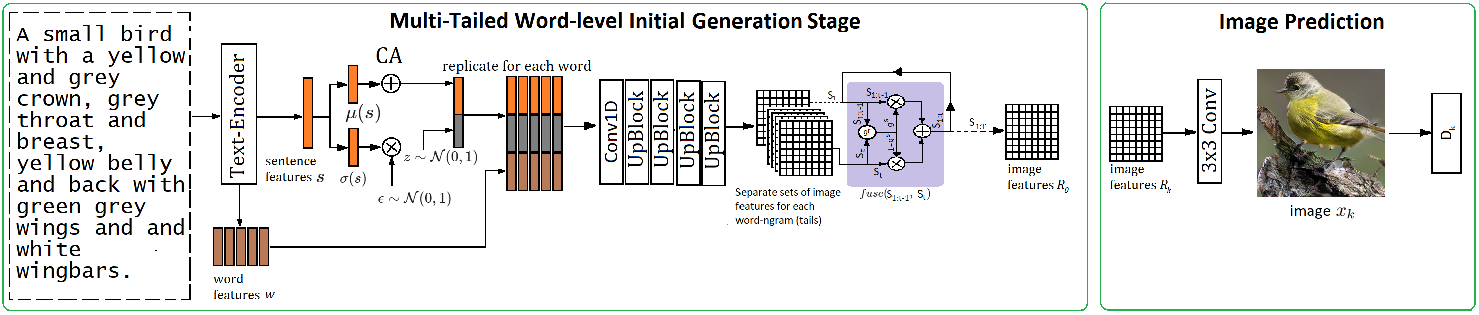
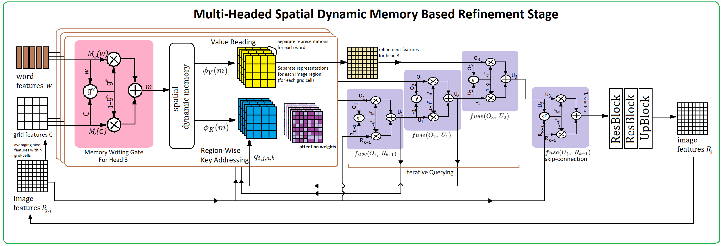
Figure 1: Our MSMT-GAN architecture for text-to-image synthesis, showing a Mutli-Tailed Word-level Initial Generation stage, a Multi-Headed Spatial Dynamic Memory based refinement stage with three refinement heads, and image prediction.

3.1 Multi-Tailed Word-level Initial Generation (MTWIG)

We highlight that previous multi-stage methods (Zhang et al., 2017; 2018; Li et al., 2019a; Zhu et al., 2019) all rely on the same type of initial generation stage and focus only on improving the refinement stages - making the conventional assumption that the performance of multi-stage generators is primarily determined by the refinement stages, and that the quality of the "rough initial image" is of little importance. In our paper, we break from this tradition and demonstrate for the first time that gains can be achieved in the final stage of image refinement by making an improvement to the initial images.

The conventional approach synthesizes initial images directly from a sentence-level vector without attempting to separate image attributes at a word-level. As a result, words that are entangled at the sentence-level representation generate initial image attributes that are inherently ambiguous in nature. In our novel Multi-Tailed Word-level Initial Generation (MTWIG) stage, we overcome this shortcoming by explicitly creating separate sets of image attributes for each word n-gram.

First, we sample a vector of random noise $z$ from a normal distribution and use a pretrained text-encoder to extract a sentence-level vector and word-level vectors: $s$ and $W$ from the input text.

$$W=\{w_{1},w_{2},...,w_{L}\};\hskip 2.84544ptw_{l}\in\mathbb{R}^{N_{w}}\;\hskip 14.22636pt;\hskip 14.22636pt\;s\in\mathbb{R}^{N_{s}}\;\hskip 14.22636pt;\hskip 14.22636pt\;z_{n}\sim\mathcal{N}(0,1);\hskip 2.84544ptz\in\mathbb{R}^{N_{z}}$$ (1)

Where $L$ is the number of words in the text-description, and $N_{z}$, $N_{s}$ and $N_{w}$ are the dimensions of the noise vector, sentence vector and word vectors respectively. To mitigate over-fitting, the Conditioning Augmentation technique (Zhang et al., 2017) is used to resample the sentence-vector from an independent Gaussian distribution. This resampled sentence vector $s^{\prime}$ and the noise vector $z$ are then concatenated with each word-level vector $w_{l}$ from the input text sequence, and the sequence of concatenated vectors are passed through a 1D convolutional operation $V$ of stride 1 (see Figure 1).

$$F=V(\{concat(s^{\prime},\;z,\;w_{l})\;|\;\;\forall\;w_{l}\in W\})$$ (2)

The length $T$ of the output sequence $F$ depends on the kernel size used by $V$ and the vectors of the output sequence $f_{t}\in F$ are each separately passed through a series of upsampling blocks to generate corresponding sets of image features $S_{t}$. These sets of image features or "tails" each correspond to a different word n-gram from the input text sequence. If we use a kernel size of 1 for $V$, then each tail $S_{t}$ corresponds to a single word. If we use a kernel size of 2, then each tail $S_{t}$ corresponds to a word bi-gram, and so on. We combine our sequence of tails $\{S_{t}\}$ together in an iterative fashion using the adaptive gating fusion mechanism introduced by Zhu et al. (2019) (discussed in Section A.1).

$$S_{1:t}=fuse(S_{1:t-1},\;S_{t},\;P^{\text{MTWIG}},\rho^{\text{MTWIG}})\hskip 14.22636pt;\hskip 14.22636ptR_{1}=S_{1:T}$$ (3)

Where $P^{\text{MTWIG}}$ and $\rho^{\text{MTWIG}}$ denote parameter matrix and bias terms, $S_{1:t}$ denotes a combination of the first $t$ tails, and $S_{1:1}$ denotes the first tail $S_{1}$. The combination of all $T$ tails gives us the final image features $R_{1}$ for our initial stage. Notice that by concatenating each word vector $w_{l}$ with $s^{\prime}$ and $z$ before the 1D convolution, each tail is created with some common information, so they may learn to fuse together coherently. Each upsampling block consists of a nearest neighbor upsampling layer and a 3×3 convolution operation. An initial image is predicted from $R_{1}$ using a 3×3 convolution.

3.2 Spatial Dynamic Memory (SDM)

In this section, we describe the operation of a single refinement head. Unlike previous methods, our novel Spatial Dynamic Memory (SDM) module creates a separate region-contextualized text representations for each image region. This allows us to interpret the same text in fundamentally different ways at different parts of an image and assimilate region-contextualized information from text at each part. To begin with, we have the set of word-level vectors $W$ and image features $R_{k-1}$ from the previous stage of generation.

$${R_{k-1}=\{r_{1,1}\;,\;r_{1,2}\;,...,\;r_{s,s}\}\;;\;\hskip 2.84544ptr_{u,v}\in\mathbb{R}^{N_{r}}}$$ (4)

Where $|s\times s|$ is the number of image pixels and $N_{r}$ is the dimension of pixel features. We obtain refinement features in three steps: Memory Writing, Key Addressing and Value Reading.
   Memory Writing: First, we divide the fine-grained $s\times s$ inital image into a coarse $h\times h$ sized grid-map and average the pixel features within each grid-cell to get grid-level image features $C$.

$$C_{i,j}=\frac{1}{|p\times p|}\hskip 5.69046pt\sum_{u=(i-1)*p+1}^{i*p}\hskip 5.69046pt\sum_{v=(j-1)*p+1}^{j*p}r_{u,v}$$ (5)

Where $p=s/h$, so that $|p\times p|$ are the number of pixels represented by each grid cell. Then, we create $L\times h\times h$ memory slots $\{m_{l,i,j}\}$ - one corresponding to each word $l$ for each grid-cell $(i,j)$. These slots are our region-contextualized representations of each word, and each slot uses a separate memory writing gate $g_{l,i,j}^{w}$ to fuse information from each grid-cell $(i,j)$ with each word feature $w_{l}$.

$$g_{l,i,j}^{w}(R_{k-1},w_{L})=\sigma\left(A*w_{l}+B_{i,j}*C_{i,j}\right)$$ (6)

$$m_{l,i,j}=M_{w}(w_{l})\odot g_{l,i,j}^{w}+M_{c}(C)_{i,j}\odot(1-g_{l,i,j}^{w})$$ (7)

The grid-level features $C$ are encoded using a 2d convolution operation $M_{c}$ (with stride 1 and $N_{m}$ output filters) and we use a common 1x1 convolution operation $M_{w}$ to encode all word vectors to a $N_{m}$ dimensional space. $A$ and $B_{i,j}$ are $1\times N_{w}$ and $1\times N_{r}$ matrices respectively.
   Key Addressing: In this step, we compute attention weights $\{\alpha_{l,i,j,a,b}\}$ over our region-contextualized text-representations $\{m_{l,i,j}\}$. The dimensions $(a,b)$ index pixels within grid-cell $(i,j)$, so that each slot $m_{l,i,j}$ gets a matrix $\alpha_{l,i,j}:p\times p$ of attention weights. Each weight is computed as a similarity probability between a key-encoding of the slot: $\phi_{K}(m_{l})_{ij}$ and a query vector: $q_{i,j,a,b}$, where $\phi_{K}(.)$ is a 2d convolution operation with stride 1 and ($N_{r}+p^{2})$ output filters.

$$\alpha_{l,i,j,a,b}=\frac{\exp(\phi_{K}(m_{l})_{i,j}*q_{i,j,a,b})}{\sum_{l=1}^{L}\exp(\phi_{K}(m_{l})_{i,j}*q_{i,j,a,b})}$$ (8)

In the case of single headed image refinement, we use the previous image features $R_{k-1}$ to obtain the query vectors. A query vector $q_{i,j,a,b}$ is made up of three components, 1)A global-level query: $q^{global}$, 2)A grid-level query: $q_{i,j}^{grid}$, and 3)A pixel-level query: $q_{i,j,a,b}^{pixel}$. To obtain these three components, we encode $R_{k-1}$ using three separate 2d convolution operations: $\phi_{Q^{global}}(.)$, $\phi_{Q^{grid}}(.)$ and $\phi_{Q^{pixel}}(.)$, each with a stride of 1 and $N_{r}$ output filters.

$$Q^{global}=\phi_{Q^{global}}(R_{k-1})\;\hskip 5.69046pt;\hskip 5.69046pt\;Q^{grid}=\phi_{Q^{grid}}(R_{k-1})\;\hskip 5.69046pt;\hskip 5.69046pt\;Q^{pixel}=\phi_{Q^{pixel}}(R_{k-1})$$ (9)

Then, the average of all pixel features of $Q^{global}$ becomes the global-level query component $q^{global}$. The average of pixel features within the grid cell $(i,j)$ of $Q^{grid}$ becomes the grid-level query $q_{i,j}^{grid}$, and the pixel feature at location $(a,b)$ within grid cell $(i,j)$ is extracted from $Q^{pixel}$ to give us the pixel-level query component $q_{i,j,a,b}^{pixel}$.

$$q^{global}=\frac{1}{|s\times s|}\sum_{u=1}^{s}\sum_{v=1}^{s}Q^{global}_{u,v}\hskip 14.22636pt;\hskip 14.22636ptq^{grid}_{i,j}=\frac{1}{|p\times p|}\hskip 5.69046pt\sum_{u=(i-1)*p+1}^{i*p}\hskip 5.69046pt\sum_{v=(j-1)*p+1}^{j*p}Q^{grid}_{u,v}$$ (10)

$$q_{i,j,a,b}^{pixel}=Q^{local}_{h(i,a),\hskip 2.84544pth(j,b)}\;\hskip 14.22636pt;\hskip 14.22636pt\;h(i,a)=(i-1)*p+a$$ (11)

Where $(h(i,a),\;h(j,b))$ indexes the pixel at location $(a,b)$ within grid-cell $(i,j)$. To obtain the final query $q_{i,j,a,b}$, we concatene these three components together.
   Value Reading: In the value reading step, for each pixel $(a,b)$ within a grid-cell $(i,j)$, we compute a weighted sum of value-encoded memory slots: $\phi_{V}(m_{l})_{ij}$ along the word dimension $l$.

$$e_{i,j,a,b}=\sum_{l=1}^{L}\alpha_{l,i,j,a,b}\cdot\phi_{V}(m_{l})_{i,j}$$ (12)

$\phi_{V}(.)$ is a 2d convolution operation with stride 1 and $N_{r}$ output filters. We now have $e_{i,j}:p\times p\times N_{r}$ dimensional matrices - each of which corresponds to a single grid cell of our coarse $h\times h$ grid map. To obtain $s\times s$ fine-grained refinement features, we apply the mapping:

$$o_{h(i,a)\;,\;h(j,b)}=e_{i,j,a,b}$$ (13)

Where $h(.,\;.)$ is the function defined in Eq.11. That is, we populate each grid cell with $|p\times p|$ vectors of $N_{r}$ dimensionality. Since $p=s/h$, we are left with a set of refinement features $O=\{o_{u,v}\}$ that are made up of $|s\times s|$ vectors of $N_{r}$ dimensionality, each of which corresponds to a single pixel.

3.3 Iterative Multi-Headed Mechanism (IMHM)

Current methods generate refinement features only once at each refinement stage and attempt to address all image aspects in a single-shot. This limits the precision with which each refinement stage can learn to improve the prior image. In order to make it easier for each refinement stage to precisely address multiple image aspects, we introduce a novel iterative multi-headed mechanism that makes multiple distinct modifications to the prior image features under common discriminator feedback. Each head of our mechanism has a separate spatial dynamic memory module formed from $R_{k-1}$ and $W$. For the first refinement head, we use the previous image features $R_{k-1}$ to obtain a query matrix and extract a set of refinement features $O_{1}$ exactly as described in Section 3.2. Then, we fuse $O_{1}$ and $R_{k-1}$ using the fusion mechanism introduced by Zhu et al. (2019) (described in Section A.1) to obtain an updated set of image features $U_{1}$. If we use only a single refinement head, then this becomes our response for the refinement stage $k$. However, if we use more than one refinement head, then for the next head, we use $U_{1}$ to obtain a query matrix. That is, we follow the same mechanism outlined in Section 3.2, but replace $R_{k-1}$ with $U_{1}$ in Eq.9. Doing so, we extract a second set of refinement features $O_{2}$, and we fuse $O_{2}$ and $U_{1}$ to obtain updated image features $U_{2}$. We proceed in this iterative fashion until we have used all of our refinement heads. The final updated image features are fused with the original image features $R_{k-1}$ in a skip-connection to obtain the final response of the refinement stage $k$. That is, if we have $T$ refinement heads:

$$U_{t}=fuse(U_{t-1},\;O_{t},\;P_{t},\;\rho_{t})\;\hskip 14.22636pt;\hskip 14.22636pt\;response_{k}=fuse(U_{T},\;R_{k-1},\;P^{skip},\;\rho^{skip})$$ (14)

Notice, we use separate parameter matrix and and bias terms $P$ and $\rho$ for each fusion operation, so that we combine refinement features and image features in a custom way for each head. The, $response_{k}$ is passed through several residual blocks (He et al., 2016) and an upsampling block to obtain higher resolution image features $R_{k}$. Each block consists of a nearest neighbor upsampling layer and a 3×3 convolution operation. Finally, a refined image $x_{k}$ is predicted from $R_{k}$ using a 3×3 convolution operation.

3.4 Objective Function

The objective function for our generator network is defined as:

$$L=\lambda_{1}L_{CA}+\sum_{k=2}^{K}\lambda_{2}L_{RED_{k}}+\sum_{k=1}^{K}\left(L_{G_{k}}+\lambda_{3}L_{DAMSM_{k}}\right)$$ (15)

Where, $L_{CA}$ denotes the conditioning augmentation loss (Zhang et al., 2017), $G_{k}$ denotes the generator of the $k^{th}$ stage so that $L_{G_{k}}$ denotes the adversarial loss for $G_{k}$, $L_{RED_{k}}$ denotes our redundancy loss for the $k^{th}$ stage, and $L_{DAMSM_{k}}$ denotes the DAMSM text-image matching loss (Xu et al., 2018) for the $k^{th}$ stage. $\lambda_{1}$, $\lambda_{2}$ and $\lambda_{3}$ are hyperparameters that combine the various losses.
   Redundancy Loss: To encourage each head of a refinement stage to focus on separate image aspects, we average region-wise information of each head’s output refinement features and penalize similarity between different refinement heads. That is, for $T$ refinement heads:

$$f(t)=\frac{1}{|s\times s|}\sum_{u=1}^{s}\sum_{v=1}^{s}o_{u,v}\hskip 2.84544pt\;\hskip 14.22636pt;\hskip 14.22636pt\;L_{RED_{k}}=\sum_{i=1}^{T}\;\sum_{j=i+1}^{T}sim(f(i),f(j))$$ (16)

Where $o_{u,v}\in O_{t}\text{ in stage }k$ (see Section 3.3) and $sim$ is the cosine similarity between vectors. We call this sum of pairwise similarity $L_{RED_{k}}$ the “redundancy loss" of the $k^{th}$ refinement stage.
   Adversarial Loss: The adversarial loss for $G_{k}$ is defined as:

$$L_{G_{k}}=-\frac{1}{2}[\mathbb{E}_{x\sim p_{G_{k}}}\log D_{k}(x)+\mathbb{E}_{x\sim p_{G_{k}}}\log D_{k}(x,s)]$$ (17)

$D_{k}$ is the discriminator network for the $k^{th}$ stage of generation. The first term provides feedback on image realism independent of the input text, and the second term provides feedback on the realism of the image in light of the input text. Alternate to adversarial training of $G_{k}$, each discriminator $D_{k}$ is trained to classify images as real or fake by minimizing the discriminator loss $L_{D_{k}}$.

$${\begin{split}L_{D_{k}}=&\underbrace{-\frac{1}{2}[\mathbb{E}_{x\sim p_{data}}\log D_{k}(x)+\mathbb{E}_{x\sim p_{G_{k}}}\log(1-D_{k}(x))]}_{\text{unconditional loss}}+\underbrace{-\frac{1}{2}[\mathbb{E}_{x\sim p_{data}}\log D_{k}(x,s)+\mathbb{E}_{x\sim p_{G_{k}}}\log(1-D_{k}(x,s))]}_{\text{conditional loss}}\end{split}}$$ (18)

Where the unconditional component distinguishes synthetic and real images independent of the input text, and the conditional component distinguishes them in light of the input text.

4 Experiments

Datasets: We evaluate our method on the Caltech-UCSD Birds 200 (CUB) dataset (Wah et al., 2011) and the Microsoft Common Objects in Context (COCO) dataset (Lin et al., 2014). The CUB dataset contains 8,855 training images and 2,933 test images, with 10 corresponding text descriptions for each image. The COCO dataset, contains 82,783 training images and 40,504 test images, with 5 corresponding text descriptions for each image. We preprocess the datasets according to the methods introduced by Zhang et al. (2017).

Evaluation metrics: To evaluate the realism of images, we rely on the Fréchet Inception Distance (FID) (Heusel et al., 2017). FID computes the distance between synthetic and real-world image distributions based on features extracted from a pre-trained Inception v3 network. A lower FID indicates greater image-realism. To evaluate the relevance of a synthetic image to it’s generating text-description, we rely on the R-precision introduced by Xu et al. (2018). R-precision is computed as the mean accuracy of using each synthetic image to retrieve one ground truth text-description from among 100 candidates. To evaluate a model on a dataset, we generate 30,000 synthetic images conditioned on text descriptions from the unseen test set.

Implementation Details: To obtain a sentence-level vector and word-level vectors for a given text description, we use the pretrained bidirectional LSTM text encoder employed by AttnGAN (Xu et al., 2018). Our MTWIG stage synthesizes images features with 64x64 resolution. Two refinement stages refine these features to 128x128 and 256x256 resolution respectively. At refinement stages, we use $T=6$ refinement heads and we use $h=8$ to divide each input image into a coarse $8\times 8$ grid map. We use the same discriminator network architecture employed by Zhu et al. (2019). Further implementation details are provided in Section A.3.

4.1 Ablative Experiments

Effectiveness of Multi-Tailed Word-level Initial Generation: In our experiments (Appendix A.1), we find that our MTWIG stage is most effective when used with a kernel size of 3, so that we generate a separate tail for each word tri-gram. To evaluate the effectiveness of our MTWIG(ks=3) stage in multi-stage models, we train our MTWIG(ks=3) method with DM-GAN (Zhu et al., 2019) style-refinement stages for 700 epochs on the CUB dataset, and observe that it decreases the FID score achieved by the original DM-GAN model by 7.72% and increases R-precision by 2.76% (Table 1). Figure 2 shows the improved visual quality of the refined images. We again point out that previous multi-stage methods (Zhang et al., 2017; 2018; Xu et al., 2018; Li et al., 2019a; Zhu et al., 2019)) all rely on the same type of initial generation stage, and we expect a similar boost in performance if we replace their initial stage with our MTWIG stage.

Effectiveness of Spatial Dynamic Memory: In order to evaluate the effectiveness of our SDM based-refinement stages, we compare a multi-stage model that uses our MTWIG(ks=3) stage and DM-GAN’s refinement stages against a multi-stage model that uses our MTWIG(ks=3) stage and our single-headed SDM-based refinement stages. Both models are trained on the CUB dataset for 700 epochs. We observe that our SDM-based refinement out-performs DM-GAN’s refinement, decreasing FID score by 4.64 % , and boosting R-precision by an additional 0.83% (Table 1). Figure 2 shows that SDM-based refinement generates images of better visual quality than those formed by DM-GAN’s refinement stages for the same initial generation architecture.

Effectiveness of the Iterative Multi-Headed Mechanism: To evaluate the effectiveness of our IMHM refinement, we compare the model that uses MTWIG(ks=3) and single-headed SDM-based refinement stages against our full MSMT-GAN model - that uses MTWIG(ks=3) and six SDM-based refinement heads for each stage. As before, both models are trained for 700 epochs on the CUB dataset. We find that refinement stages that use our multi-headed mechanism out-perform single-headed refinement stages, decreasing FID score 2.38%, and boosting R-precision by another 1.03% (Table 1). Visually, besides overall better image quality, we find that images generated by multi-headed refinement stages posess text-irrelevant content that is far more detailed than that observed in images generated by single-headed refinement stages (Figure 2).

Table 1: FID and R-precision of DM-GAN and ablative versions of our model. (With all of our variants trained for 700 epochs on CUB)

CUB
Method	FID $\downarrow$	R-prcn (%) $\uparrow$
DM-GAN	11.91	76.58 ± 0.53
MTWIG w/ DM-GAN’s refinement	10.99	79.37 ± 0.73
MTWIG w/ SDM refinement	10.48	80.20 ± 0.67
MTWIG w/ SDM and IMHM refinement (MSMT-GAN)	10.23	81.23 ± 0.68

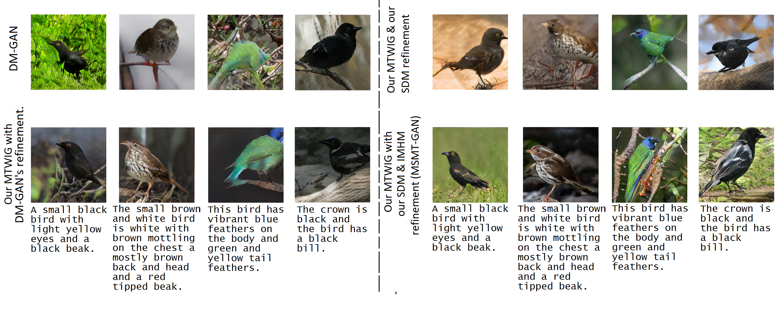
Figure 2: Comparison of DM-GAN with ablative versions of our model trained for 700 epochs on the CUB dataset.

4.2 Comparison with State of the Art

To compare our architecture against the previous state-of-the-art for the task of text-to-image generation, we train MSMT-GAN models for 1000 epochs on the CUB dataset and for 210 epochs on the COCO dataset. As shown in Table 3, our MSMT-GAN decreases the previous lowest reported FID score by 21.58% on the CUB dataset -marking a significant improvement in image realism, and also boosts the previous best reported CUB R-precision by 4.24 % - marking a large improvement in the similarity of synthetic images to their generating text. As shown in Table 2 and Table 3, our model is comparable in size to previous methods, and outperforms the next closest contender of similar size for COCO (DM-GAN) by 4.21% on FID score -making it highly competitive with the current state-of-the-art. We also observe a slight improvement of 0.23% on COCO R-precision. Qualitatively, we observe that synthetic images generated by our model are typically sharper and more realistic than those generated by prior methods (Figure 3). In particular, we observe that our method generates synthetic images that possess greater detail and that are better matches for the generating text.

Table 2: Number of parameters required at test-time (including text-encoders) for the previous state-of-the-art in comparison to our MSMT-GAN (approximate values reported in millions).

Method	# Paramers for CUB	# Parameters for COCO
AttnGAN	9.16M	22.43M
ControlGAN	30.72M	45.36M
DM-GAN	23.52M	30.96M
DF-GAN	14.32M	20.87M
XMC-GAN	-	>111M
Our MSMT-GAN	48.11M	55.16M

Table 3: FID and R-precision of the previous state-of-the-art and our MSMT-GAN trained for 1000 epochs on CUB and 210 epochs on COCO.

CUB		COCO
Method	FID $\downarrow$	R-prcn (%) $\uparrow$	FID $\downarrow$	R-prcn (%) $\uparrow$
AttnGANA.4	14.01	67.82 ± 4.43	29.53	85.47 ± 3.69
ControlGAN	-	69.33 ± 3.23	-	82.43 ± 2.43
DM-GANA.4	11.91	76.58 ± 0.53	24.24	92.23 ± 0.37
DF-GANA.4	13.48	-	33.29	-
Our MSMT-GAN	9.34	80.82 ± 0.54	23.22	92.46 ± 0.28

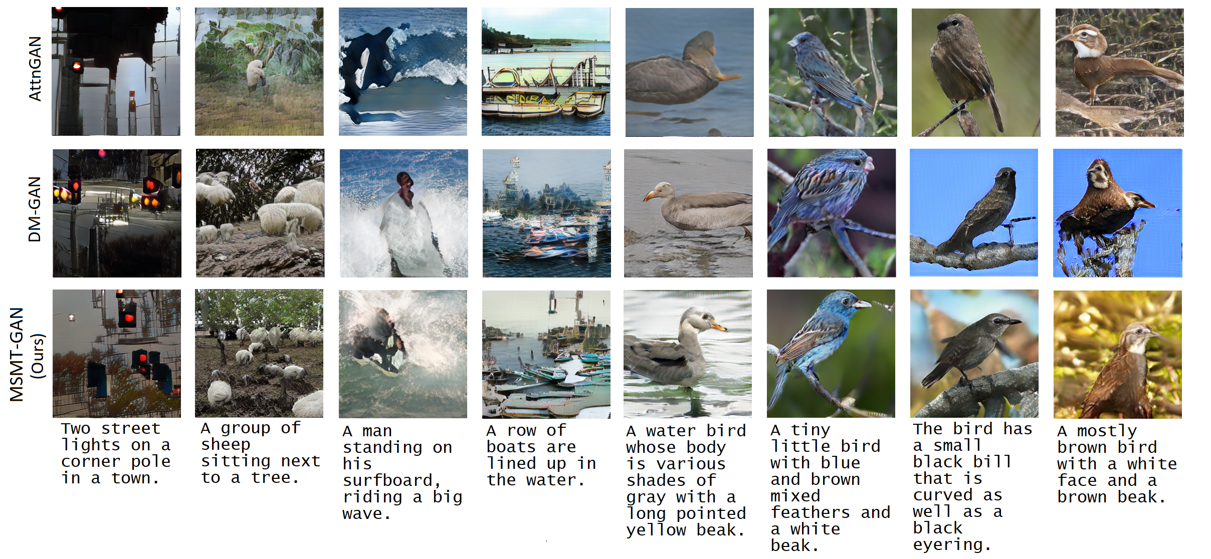
Figure 3: Comparison of MSMT-GAN with state-of-the art models on the CUB and COCO datasets.

5 Conclusion

In this work, we have proposed the MSMT-GAN architecture for the task of text-to-image synthesis. First, we introduced a novel Multi-Tailed Word Level Initial Generation stage (MTWIG) that explicitly generates separate sets of image features for each word n-gram. Second, we proposed a novel Spatial Dynamic Memory (SDM) module to contextualize text representations by image-region. Third, we introduced a novel Iterative Multi-Headed Mechanism (IMHM) of image refinement to make it easier for each refinement stage to precisely address multiple image aspects. Our ablative experiments clearly demonstrate the effectiveness each of these three components, and we have shown that we are able to boost the performance of prior methods by replacing their initial stage with our MTWIG stage. Experiment results further demonstrate that our MSMT-GAN model significantly out-performs the previous state of the art on the CUB dataset, decreasing the lowest reported FID score by 21.58% and boosting the CUB R-precision by 4.24%. On the COCO dataset, we have demonstrated that MSMT-GAN is highly comptitive with current methods based on image realism and model size. In future work, we aim to design a discriminator model that provides more region-specific feedback than existing methods, to use in conjunction with our MSMT-GAN generator architecture.

6 Acknowledgements

This work was performed while Amrit Diggavi Seshadri was a Post Baccalaureate Fellow at the Robert Bosch Center for Data Science and Artificial Intelligence (RBC-DSAI), at the Indian Institute of Technology Madras (IIT Madras). We would like to thank the center for sponsoring this fellowship and for providing us with sufficient resources.

Appendix A Appendix

A.1 Fusing two sets of image features together

Given any two sets of image/refinement features $A=\{a_{u,v}\}$ and $B=\{b_{u,v}\}$ such that $a_{u,v},\;b_{u,v}\in\mathbb{R}^{N_{r}}$, we can use the adaptive gating mechanism introduced by Zhu et al. (2019) to obtain a combined/updated set of features $\{r_{u,v}\}$, where $r_{u,v}\in\mathbb{R}^{N_{r}}$.

$$g^{r}_{u,v}=\sigma(P*concat(a_{u,v},\;b_{u,v})+\rho)$$ (19)

$$r_{u,v}=a_{u,v}\odot g^{r}_{u,v}+b_{u,v}\odot(1-g^{r}_{u,v})$$ (20)

Where $(u,v)$ index pixel locations, $N_{r}$ is the dimension of image pixel features, $g^{r}_{u,v}$ is a gate for information fusion, $\sigma$ is the sigmoid function and $P$ and $\rho$ are the parameter matrix and bias term respectively. In our paper, we invoke this adaptive gating mechanism by a function “$fuse$" such that $fuse(A,B,P,\rho)=\{r_{u,v}\}$.

A.2 Analysis of Multi-Tailed Word-level Initial Generation

Table 4: Quantitative comparison of Fréchet Inception Distance and R-precision between previous Initial Generation (IG) and our Multi-Tailed Word-level Initial Generation (MTWIG) stage for varied kernel sizes (ks) on the CUB and COCO datasets.

CUB		COCO
Method	FID $\downarrow$	R-prcn (%) $\uparrow$	FID $\downarrow$	R-prcn (%) $\uparrow$
IG	119.39	83.54 ± 0.57	51.22	94.57 ± 0.53
MTWIG (ks=1)	118.49	82.78 ± 0.58	41.79	94.47 ± 0.49
MTWIG (ks=2)	120.76	82.82 ± 0.92	40.23	94.65 ± 0.39
MTWIG (ks=3)	115.38	82.94 ± 0.74	39.85	94.80 ± 0.29

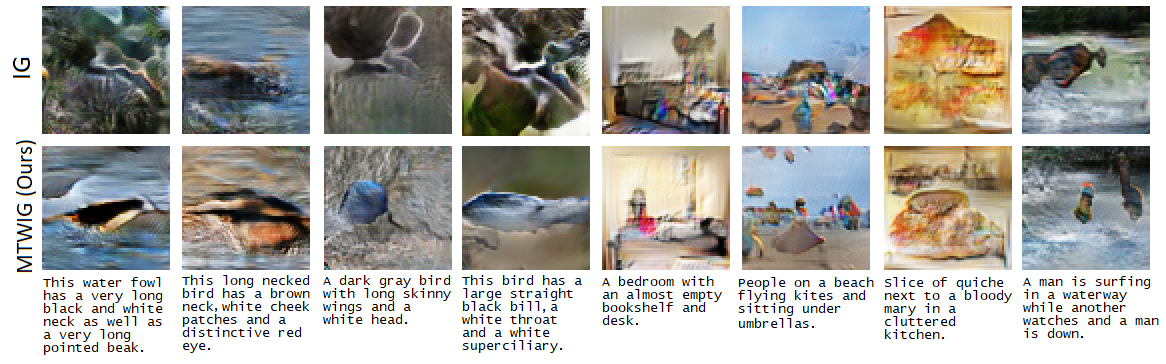
Figure 4: Multi-Tailed Word-level Initial Generation (MTWIG; kernel size=3) in comparison to conventional Initial Generation (IG).

To analyze the effectiveness of our MTWIG stage, we make comparisons with the inital generation (IG) stage employed by previous methods (Zhang et al., 2017; 2018; Xu et al., 2018; Li et al., 2019a; Zhu et al., 2019). We train IG and MTWIG stages without refinement for 300 epochs on the CUB dataset and for 60 epochs on the COCO dataset. Table 4 shows a quantitative comparison between IG and MTWIG architectures that use different kernel sizes. We observe that our MTWIG method achieves best results for ks=3 (that is, by forming separate sets of word tri-grams), decreasing FID scores from the previous IG method by 3.36% on the CUB dataset and by 22.2% on the COCO dataset. The larger improvement observed on the COCO dataset highlights that our MTWIG method is most beneficial for complex scene generation, where the presence of a large number of distinct objects demands word-level separation of attributes. Our MTWIG stages also achieves competitive R-precision scores on both datasets, demonstrating that images synthesized by our method are well conditioned on their input text-descriptions. In Figure 4, we visually compare 64x64 images generated by IG and images generated by our MTWIG(ks=3) model. We observe that images generated by our method typically posses object attributes that are better separated and more clearly discernible.

A.3 Additional Implementation Details

We set $N_{w}=256$, $N_{r}=48$ and $N_{m}=96$ to be the dimension of text, image and memory feature vectors respectively. We set the hyperparameters $\{\lambda_{1}=1,\;\lambda_{2}=0.5,\;\lambda_{3}=5\}$ for the CUB dataset and $\{\lambda_{1}=1,\;\lambda_{2}=0.5,\;\lambda_{3}=50\}$ for the COCO dataset. All networks are trained using an ADAM optimizer (Kingma & Ba, 2015) with $\beta_{1}=0.5$ and $\beta_{2}=0.999$. The learning rate is set to be 0.0002 and we use a batch size of 20 for all networks. We train our models on a single Tesla V100 gpu, and observe that similar to previous multi-stage methods, training our MSMT-GAN method is a GPU intensive process. We require approximately 27min for one epoch of the CUB dataset, and approximately 4.7 hours for one epoch of the COCO dataset.

A.4 Note on Evaluation Metrics

We point out that there is inconsistency in the FID implementation used to evaluate prior methods. While some methods (Li et al., 2019b) report scores using the official Tensorflow version of FID - which uses the weights of a pretrained Tensorflow inception model, other methods (Zhu et al., 2019; Zhang et al., 2021) have reported scores using an unofficial Pytorch implementation of FID - that uses the weights of a pretrained Pytorch inception model.

Each of these implementations computes different values of FID scores for the same sets of images, and scores computed from the two versions are not directly comparable with each other. We highlight that the correlation between FID score and human judgement is an empirical observation, that is dependent on the weights of the pretrained inception model used. The correlation with human judgement has only been shown to hold true for the weights of the pretrained Tensorflow inception model (used by the FID authors -Heusel et al. (2017)), and has not been verified for the unofficial Pytorch inception model (which has different weights). As such, to ensure that we correlate with human judgement, in our paper we only report scores using the official Tensorflow implementation of FID score - computing values for prior work from the pretrained models released by their authors. In Table 5 below, we additionally report Pytorch-implementation FID scores of SEGAN (Tan et al., 2019) and XMC-GAN (Zhang et al., 2021) models, as reported by their authors. It was not possible for us to recompute these scores using the official Tensorflow version of FID as pretrained models for these methods have not been made publicly available.

We again highlight, that the FID scores computed by the official Tensorflow implementation are not directly comparable with the scores computed by the unofficial Pytorch implementation.

In Table 5, we additionally benchmark the performance of models on the Inception Score (IS) (Goodfellow et al., 2014). We note however, that the FID score (which is reference-based and compares the distributions of real and synthetic images together) has been observed to be more consistent with human judgement of image realism than IS (which is reference-free and does not make comparisons to real images) (Heusel et al., 2017). We were not able to recompute other metrics for RiFeGAN (Cheng et al., 2020) and LeciaGAN (Qiao et al., 2019) as the pretrained models have not been made publicly available.

Table 5: FID and R-precision and IS of the previous methods and our MSMT-GAN trained for 1000 epochs on CUB and 210 epochs on COCO.

CUB			COCO
Method	FID $\downarrow$	R-prcn (%) $\uparrow$	IS $\uparrow$	FID $\downarrow$	R-prcn (%) $\uparrow$	IS $\uparrow$
AttnGANA.4	14.01	67.82 ± 4.43	4.36 ± 0.03	29.53	85.47 ± 3.69	25.89 ± 0.47
ControlGAN	-	69.33 ± 3.23	4.58 ± 0.09	-	82.43 ± 2.43	24.06 ± 0.60
SEGAN	18.16A.4	-	4.67 ± 0.04	32.28	-	27.86 ± 0.31
RiFeGAN	-	-	5.23 ± 0.09	-	-	-
LeciaGAN	-	-	4.62 ± 0.06	-	-	-
DM-GANA.4	11.91	76.58 ± 0.53	4.71 ± 0.06	24.24	92.23 ± 0.37	32.43 ± 0.58
DF-GANA.4	13.48	-	4.70 ± 0.06	33.29	-	18.64 ± 0.64
XMC-GAN	-	-	-	9.33A.4	-	30.45
Our MSMT-GAN	9.34	80.82 ± 0.54	4.55 ± 0.06	23.22	92.46 ± 0.28	28.91 ± 0.35

In Table 5, “-” represents cases where the data was not reported or is reported in a manner which is non-comparable (besides FID values).

A.5 More example images

Figures 5 and 6 below show more images generated by our method in comparison to prior work on the CUB and COCO datasets. Again, we observe that synthetic images generated by MSMT-GAN are typically sharper and more realistic than those generated by previous methods. We also observe that the synthetic images generated by MSMT-GAN are usually a better match for the generating text.

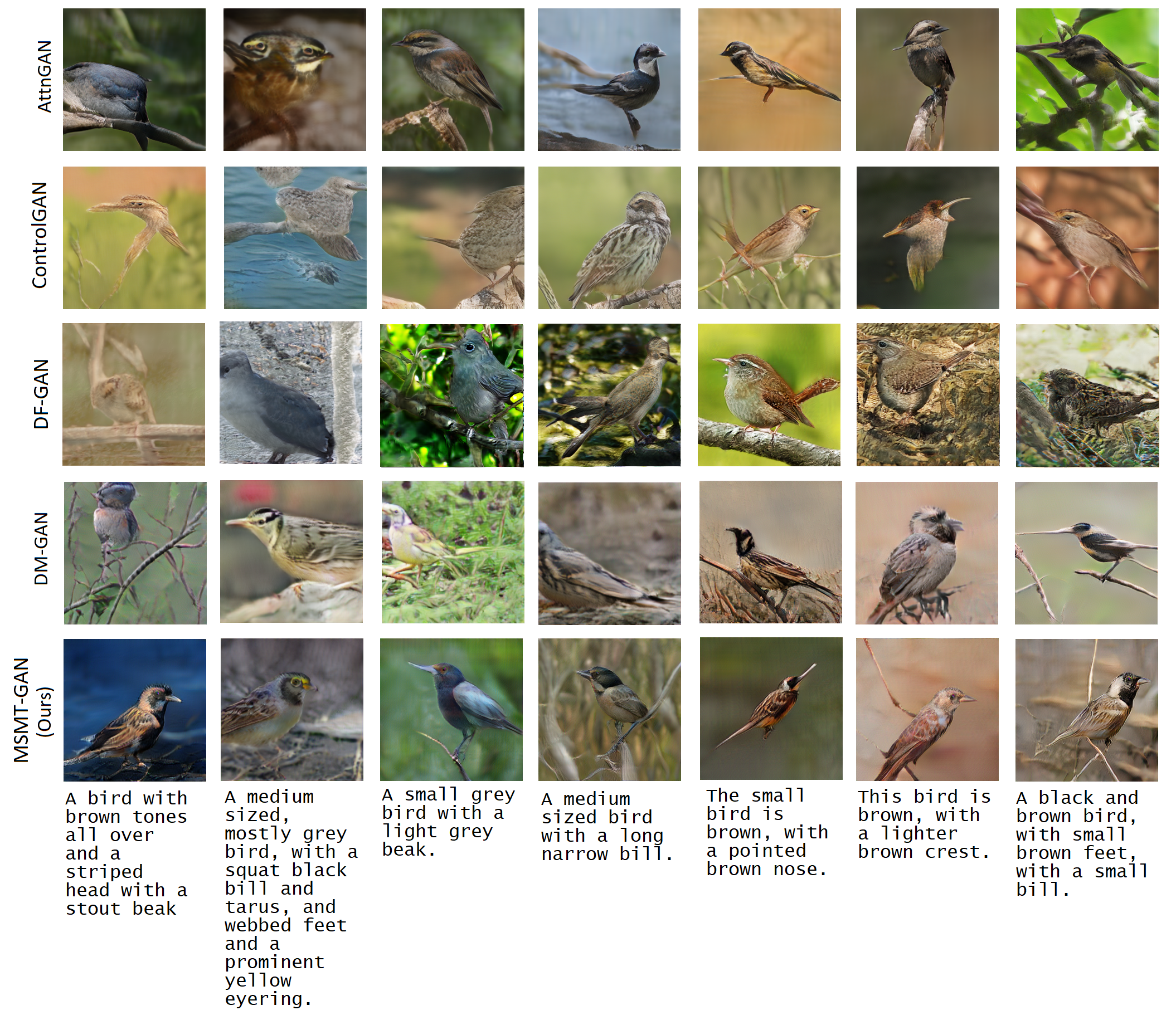
Figure 5: Extended comparison of MSMT-GAN with state-of-the art models on the CUB dataset.

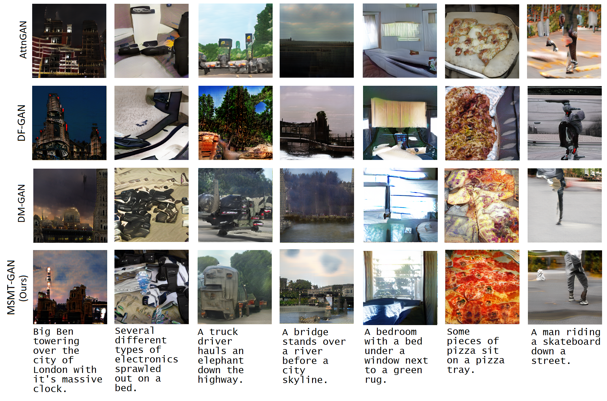
Figure 6: Extended comparison of MSMT-GAN with state-of-the art models on the COCO dataset.

References

- Cheng et al. (2020) Jun Cheng, Fuxiang Wu, Yanling Tian, Lei Wang, and Dapeng Tao. Rifegan: Rich feature generation for text-to-image synthesis from prior knowledge. In Proceedings of the IEEE/CVF Conference on Computer Vision and Pattern Recognition, pp. 10911–10920, 2020.
- Cho et al. (2020) Jaemin Cho, Jiasen Lu, Dustin Schwenk, Hannaneh Hajishirzi, and Aniruddha Kembhavi. X-lxmert: Paint, caption and answer questions with multi-modal transformers. arXiv preprint arXiv:2009.11278, 2020.
- Denton et al. (2015) Emily L Denton, Soumith Chintala, Rob Fergus, et al. Deep generative image models using a laplacian pyramid of adversarial networks. In Advances in neural information processing systems, pp. 1486–1494, 2015.
- Goodfellow et al. (2014) Ian Goodfellow, Jean Pouget-Abadie, Mehdi Mirza, Bing Xu, David Warde-Farley, Sherjil Ozair, Aaron Courville, and Yoshua Bengio. Generative adversarial nets. In Advances in neural information processing systems, pp. 2672–2680, 2014.
- He et al. (2016) Kaiming He, Xiangyu Zhang, Shaoqing Ren, and Jian Sun. Deep residual learning for image recognition. In Proceedings of the IEEE conference on computer vision and pattern recognition, pp. 770–778, 2016.
- Heusel et al. (2017) Martin Heusel, Hubert Ramsauer, Thomas Unterthiner, Bernhard Nessler, and Sepp Hochreiter. Gans trained by a two time-scale update rule converge to a local nash equilibrium. In Advances in neural information processing systems, pp. 6626–6637, 2017.
- Hinz et al. (2019) Tobias Hinz, Stefan Heinrich, and Stefan Wermter. Semantic object accuracy for generative text-to-image synthesis. arXiv preprint arXiv:1910.13321, 2019.
- Kingma & Ba (2015) Diederik P Kingma and Jimmy Ba. Adam: A methodfor stochastic optimization. In International Conference onLearning Representations (ICLR), 2015.
- Li et al. (2019a) Bowen Li, Xiaojuan Qi, Thomas Lukasiewicz, and Philip Torr. Controllable text-to-image generation. In Advances in Neural Information Processing Systems, pp. 2065–2075, 2019a.
- Li et al. (2019b) Wenbo Li, Pengchuan Zhang, Lei Zhang, Qiuyuan Huang, Xiaodong He, Siwei Lyu, and Jianfeng Gao. Object-driven text-to-image synthesis via adversarial training. In Proceedings of the IEEE/CVF Conference on Computer Vision and Pattern Recognition, pp. 12174–12182, 2019b.
- Liang et al. (2020) Jiadong Liang, Wenjie Pei, and Feng Lu. Cpgan: Content-parsing generative adversarial networks for text-to-image synthesis. In European Conference on Computer Vision, pp. 491–508. Springer, 2020.
- Lin et al. (2014) Tsung-Yi Lin, Michael Maire, Serge Belongie, James Hays, Pietro Perona, Deva Ramanan, Piotr Dollár, and C Lawrence Zitnick. Microsoft coco: Common objects in context. In European conference on computer vision, pp. 740–755. Springer, 2014.
- Miller et al. (2016) Alexander Miller, Adam Fisch, Jesse Dodge, Amir-Hossein Karimi, Antoine Bordes, and Jason Weston. Key-value memory networks for directly reading documents. arXiv preprint arXiv:1606.03126, 2016.
- Qiao et al. (2019) Tingting Qiao, Jing Zhang, Duanqing Xu, and Dacheng Tao. Learn, imagine and create: Text-to-image generation from prior knowledge. Advances in Neural Information Processing Systems, 32:887–897, 2019.
- Radford et al. (2015) Alec Radford, Luke Metz, and Soumith Chintala. Unsupervised representation learning with deep convolutional generative adversarial networks. arXiv preprint arXiv:1511.06434, 2015.
- Reed et al. (2016) Scott Reed, Zeynep Akata, Xinchen Yan, Lajanugen Logeswaran, Bernt Schiele, and Honglak Lee. Generative adversarial text to image synthesis. arXiv preprint arXiv:1605.05396, 2016.
- Salimans et al. (2016) Tim Salimans, Ian Goodfellow, Wojciech Zaremba, Vicki Cheung, Alec Radford, and Xi Chen. Improved techniques for training gans. Advances in neural information processing systems, 29:2234–2242, 2016.
- Tan et al. (2019) Hongchen Tan, Xiuping Liu, Xin Li, Yi Zhang, and Baocai Yin. Semantics-enhanced adversarial nets for text-to-image synthesis. In Proceedings of the IEEE/CVF International Conference on Computer Vision, pp. 10501–10510, 2019.
- Vaswani et al. (2017) Ashish Vaswani, Noam Shazeer, Niki Parmar, Jakob Uszkoreit, Llion Jones, Aidan N Gomez, Łukasz Kaiser, and Illia Polosukhin. Attention is all you need. In Advances in neural information processing systems, pp. 5998–6008, 2017.
- Wah et al. (2011) Catherine Wah, Steve Branson, Peter Welinder, Pietro Perona, and Serge Belongie. The caltech-ucsd birds-200-2011 dataset. 2011.
- Weston et al. (2014) Jason Weston, Sumit Chopra, and Antoine Bordes. Memory networks. arXiv preprint arXiv:1410.3916, 2014.
- Xu et al. (2018) Tao Xu, Pengchuan Zhang, Qiuyuan Huang, Han Zhang, Zhe Gan, Xiaolei Huang, and Xiaodong He. Attngan: Fine-grained text to image generation with attentional generative adversarial networks. In Proceedings of the IEEE conference on computer vision and pattern recognition, pp. 1316–1324, 2018.
- Zhang et al. (2017) Han Zhang, Tao Xu, Hongsheng Li, Shaoting Zhang, Xiaogang Wang, Xiaolei Huang, and Dimitris N Metaxas. Stackgan: Text to photo-realistic image synthesis with stacked generative adversarial networks. In Proceedings of the IEEE international conference on computer vision, pp. 5907–5915, 2017.
- Zhang et al. (2018) Han Zhang, Tao Xu, Hongsheng Li, Shaoting Zhang, Xiaogang Wang, Xiaolei Huang, and Dimitris N Metaxas. Stackgan++: Realistic image synthesis with stacked generative adversarial networks. IEEE transactions on pattern analysis and machine intelligence, 41(8):1947–1962, 2018.
- Zhang et al. (2021) Han Zhang, Jing Yu Koh, Jason Baldridge, Honglak Lee, and Yinfei Yang. Cross-modal contrastive learning for text-to-image generation. In Proceedings of the IEEE/CVF Conference on Computer Vision and Pattern Recognition, pp. 833–842, 2021.
- Zhu et al. (2019) Minfeng Zhu, Pingbo Pan, Wei Chen, and Yi Yang. Dm-gan: Dynamic memory generative adversarial networks for text-to-image synthesis. In Proceedings of the IEEE Conference on Computer Vision and Pattern Recognition, pp. 5802–5810, 2019.