Abstract

The increasing share of volatile renewable electricity production motivates demand response. Substantial potential for demand response is offered by flexible processes and their local multi-energy supply systems. Simultaneous optimization of their schedules can exploit the demand response potential, but leads to numerically challenging problems for nonlinear dynamic processes. In this paper, we propose to capture process dynamics using dynamic ramping constraints. In contrast to traditional static ramping constraints, dynamic ramping constraints are a function of the process state and can capture high-order dynamics. We derive dynamic ramping constraints rigorously for the case of single-input single-output processes that are exactly input-state linearizable. The resulting scheduling problem can be efficiently solved as a mixed-integer linear program. In a case study, we study two flexible reactors and a multi-energy system. The proper representation of process dynamics by dynamic ramping allows for faster transitions compared to static ramping constraints and thus higher economic benefits of demand response. The proposed dynamic ramping approach is sufficiently fast for application in online optimization.

• Forschungszentrum Jülich GmbH, Institute of Energy and Climate Research, Energy Systems Engineering (IEK-10), Jülich 52425, Germany

• RWTH Aachen University Aachen 52062, Germany

• ETH Zürich, Energy & Process Systems Engineering, Zürich 8092, Switzerland

Keywords:
Demand response, Mixed-integer dynamic optimization, Exact linearization, Scheduling optimization

Highlights:

• Dynamic ramping constraints for scheduling of processes and energy systems

• Allow for high-order dynamics, and non-constant ramp limits

• Derived rigorously from exact input-state linearization

• Mixed-integer linear optimization fast enough for online optimization

• Cost savings close to nonlinear optimization

1 Introduction

Many countries are transforming their national energy systems towards renewable energies. This transformation requires more renewable electricity generation by wind and sun. The inherent volatility of renewable electricity generation causes temporal imbalances of demand and supply. These imbalances can be reduced if consumers shift their demand in time. Ideally, both electricity grid and consumers benefit from this demand response (DR) (Zhang and Grossmann,, 2016). To incentivize demand shifting for consumers, electricity is traded with time-varying prices at day-ahead and intra-day markets. At these markets prices react to the current demand and supply.

Demand response is especially promising for the chemical industry. Many energy-intensive production processes offer demand response potential, i.e., these processes can (i) adjust their production rate and thus energy demand, and (ii) store their product for later use (Mitsos et al.,, 2018; Merkert et al.,, 2015). However, chemical processes consume different forms of energy – not only electricity, but also cooling, or heating. Therefore, processes are typically supplied by a local multi-energy system which consumes primary energy sources and exchanges electricity with the grid, either by buying electricity from the grid or by selling electricity from on-site production (Voll et al.,, 2013). Consequently, DR needs to consider both the process and its local energy system in a simultaneous scheduling (Agha et al.,, 2010; Leenders et al.,, 2019; Baader et al., 2022c, ) (Figure 1) that determines operational set points for a time horizon in the order of one day (Baldea and Harjunkoski,, 2014).

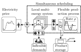
Figure 1: Simultaneous scheduling of a flexible production process and its local multi-energy system reacts to variable electricity prices using the demand response potential of the process by modulating the production rate $\rho$ and thus process energy consumption.

The desired simultaneous scheduling leads to computationally intensive optimization problems because processes and energy systems introduce two different challenges that are hard to solve simultaneously: First, processes often introduce scheduling-relevant nonlinear dynamics (Mitsos et al.,, 2018; Baldea and Harjunkoski,, 2014; Daoutidis et al.,, 2018; Caspari et al.,, 2019; Otashu and Baldea,, 2019). Scheduling-relevant means the time that the process needs to change between two steady states is in the same order of magnitude as electricity price time steps, e.g., 1 hour. Second, energy system models often introduce discrete decision variables resulting from often redundant units with minimum part-load constraints (Voll et al.,, 2013). Thus, the resulting problems are mixed-integer nonlinear dynamic optimization problems which are notoriously difficult to solve. However, scheduling optimization must be performed online in order to timely provide operational set-points for the underlying control. The maximum allowed optimization runtime is typically between 5 and 20 minutes (Iiro Harjunkoski et al.,, 2014). To achieve such runtimes, the optimization problem needs to be reformulated to a simpler problem.

Online-applicable optimization runtimes of local energy systems alone can often be achieved by mixed-integer linear programming (MILP) formulations (Risbeck et al.,, 2017; Mitra et al.,, 2013; Carrion and Arroyo,, 2006; Sass et al.,, 2020). The MILP problem can also integrate the production process if the process has negligible dynamics such that quasi-steady-state assumptions can be used on the scheduling time scale. Scheduling can then calculate a feasible trajectory of operational set-points. Based on this trajectory, the real process inputs are determined by the underlying control (Baldea and Harjunkoski,, 2014). Accordingly, for negligible process dynamics, no process model is needed but only the process energy demands must be described as piece-wise affine function of the production rate (Schäfer et al.,, 2020; Brée et al.,, 2019).

For processes with relevant dynamics, scheduling optimization still does not necessarily need to consider the full-order process model but rather requires a set of constraints that determine how fast the process can change its production rate. Traditional first-order ramping constraints bound the first derivative of the production rate using constant limits (Carrion and Arroyo,, 2006) but have two shortcomings for simultaneous scheduling that we address in this paper: First, constant ramping limits cause either unnecessarily conservative or infeasible schedules if the achievable rate of change varies with the process state (T. Li and M. Shahidehpour,, 2007; C. M. Correa-Posada et al.,, 2017), which is typical for nonlinear chemical processes. Second, first-order dynamics may not be applicable. If, for example, a chemical reactor has a temperature-dependent production rate and is cooled through a reactor jacket with a significant thermal inertia, changing the production rate through a change of reactor temperature would lead to at least second-order dynamics.

To overcome both shortcomings, we propose high-order dynamic ramping constraints for simultaneous DR scheduling of processes and energy systems. For this purpose, we present a method to rigorously derive such dynamic ramping constraints for the case of exact input-state linearizable single-input single-output (SISO) processes based on the full-order nonlinear process model. Our high-order dynamic ramping constraints are based on a chain of differential equations. The highest considered time-derivative is the ramping degree of freedom that is limited by dynamic limits as function of the process state. With time discretization by collocation (Biegler,, 2010), these high-order dynamic ramping constraints can be converted to linear algebraic constraints and thus allow for an MILP formulation. Thus, dynamic ramping constraints can be readily integrated into typical MILP-based energy system optimization models (Sass et al.,, 2020).

The remaining paper is structured as follows: In Section 2, we introduce the original nonlinear optimization problem for simultaneous scheduling and the reformulated linear optimization problem with dynamic ramping constraints. In Section 3, we present a rigorous derivation of dynamic ramping constraints from exact input-state linearization for SISO processes. In Section 4, a case study featuring two continuous stirred tank reactors (CSTRs) and a multi-energy system is investigated. In Section 5, we discuss possible extensions for cases that are not covered by our current assumptions. Section 6 concludes the work.

2 Simultaneous dynamic scheduling of process and energy system

In Section 2.1, we present the original simultaneous dynamic scheduling problem (P1) which is a nonlinear mixed-integer dynamic optimization (MIDO) problem. In Section 2.2, we introduce the proposed MILP problem formulation (P2) based on high-order dynamic ramping constraints.

2.1 Nonlinear mixed-integer dynamic scheduling

In the original scheduling optimization problem (P1), all decision variables $\bm{\chi}=(\mathbf{x}^{T},\mathbf{u}^{T},(\mathbf{Q}_{\text{dem}}^{\text{process}})^{T},\rho,S,$ $\Phi_{\text{energy}},(\mathbf{Q}^{\text{in}})^{T},(\mathbf{Q}^{\text{out}})^{T},(\Delta\mathbf{P})^{T},\mathbf{z}_{\text{on}}^{T})^{T}$, which are further explained in the following, are functions of time $t$ although not stated explicitly to improve readability. We use the notation $\dot{\chi}$ to indicate the first time derivative of a variable $\chi$, and $\chi^{(k)}$ to indicate the $k$-th time derivative. The problem reads:

$$\hskip 56.9055pt\underset{\bm{\chi}\in\left[\bm{\chi}^{l},\bm{\chi}^{u}\right]}{\text{min}}\leavevmode\nobreak\ \leavevmode\nobreak\ \Phi_{\text{energy}}(t_{f})$$ (P1a)

s.t. Process model:

$$\dot{\mathbf{x}}=\mathbf{f}_{1}(\mathbf{x})+\mathbf{f}_{2}(\mathbf{x})\mathbf{u}\leavevmode\nobreak\ \leavevmode\nobreak\ \leavevmode\nobreak\ \forall t\in\left[t_{0},t_{f}\right]$$ (P1b)

Product quality:

$$0\geq\mathbf{g}(\mathbf{x},\rho)\leavevmode\nobreak\ \leavevmode\nobreak\ \leavevmode\nobreak\ \forall t\in\left[t_{0},t_{f}\right]$$ (P1c)

Process energy demand:

$$Q_{\text{dem},e}^{\text{process}}=h_{e}(\mathbf{x},\mathbf{u})\leavevmode\nobreak\ \forall e\in\mathbb{E},\leavevmode\nobreak\ \forall t\in\left[t_{0},t_{f}\right]$$ (P1d)

Product storage:

$$\dot{S}=\rho-\rho^{\text{nom}}\leavevmode\nobreak\ \leavevmode\nobreak\ \leavevmode\nobreak\ \forall t\in\left[t_{0},t_{f}\right]$$ (P1e)

Energy costs:

$$\dot{\Phi}_{\text{energy}}=\sum_{e\in\mathbb{E}}p_{e}\left(\sum_{i\in\mathbb{C}_{e}^{\text{cons}}}Q_{i}^{\text{in}}+\Delta P_{e}\right)\leavevmode\nobreak\ \leavevmode\nobreak\ \leavevmode\nobreak\ \forall t\in\left[t_{0},t_{f}\right]$$ (P1f)

Energy conversion:

$$Q_{i}^{\text{out}}=\eta_{i}\left(\frac{Q_{i}^{\text{out}}}{Q_{i}^{\text{max}}}\right)Q_{i}^{\text{in}}\leavevmode\nobreak\ \leavevmode\nobreak\ \leavevmode\nobreak\ \forall i\in\mathbb{C},\leavevmode\nobreak\ \forall t\in\left[t_{0},t_{f}\right]$$ (P1g)

Minimum part-load:

$$z_{i}^{\text{on}}Q_{i}^{\text{min}}\leq Q_{i}^{\text{out}}\leq z_{i}^{\text{on}}Q_{i}^{\text{max}},\leavevmode\nobreak\ \leavevmode\nobreak\ \leavevmode\nobreak\ \forall i\in\mathbb{C},\leavevmode\nobreak\ \forall t\in\left[t_{0},t_{f}\right]$$ (P1h)

$$\text{with}\leavevmode\nobreak\ z_{i}^{\text{on}}\in\{0,1\}$$

Energy balance:

$$Q_{\text{dem},e}^{\text{process}}+Q_{\text{dem},e}^{\text{inflexible}}=\sum_{i\in\mathbb{C}_{e}^{\text{sup}}}Q_{i}^{\text{out}}+\Delta P_{e}\leavevmode\nobreak\ \leavevmode\nobreak\ \leavevmode\nobreak\ \forall e\in\mathbb{E},\leavevmode\nobreak\ \forall t\in\left[t_{0},t_{f}\right]$$ (P1i)

The objective (P1a) is to minimize the cumulative energy costs $\Phi_{\text{energy}}$ at final time $t_{f}$. All decision variables are subject to upper and lower bounds, $\bm{\chi}^{u},\bm{\chi}^{l}$, respectively. The process model (P1b) of chemical production processes can usually be expressed in input-affine control form (Corriou,, 2018; Baldea and Daoutidis,, 2012), i.e., the time derivative of process states $\dot{\mathbf{x}}$ is given by two nonlinear functions $\mathbf{f}_{1}(\mathbf{x})$, $\mathbf{f}_{2}(\mathbf{x})$ and the process degrees of freedom $\mathbf{u}$. The process model is valid for all time points between initial time $t_{0}$ and final time $t_{f}$. To maintain product quality (P1c), we assume constraints $\mathbf{g}$ on process states $\mathbf{x}$ and the production rate $\rho$. The process energy demand $Q_{\text{dem},e}^{\text{process}}$ (P1d) for an energy form $e$ in the set of energy forms $\mathbb{E}$ is a function $h_{e}(\mathbf{x},\mathbf{u})$ of process states $\mathbf{x}$ and degrees of freedom $\mathbf{u}$. For product storage (P1e), we assume a buffer storage with filling level $S$. As all decision variables, the filling level $S$ is subject to upper and lower bounds. Moreover, the final storage filling level $S(t_{f})$ might be constrained to be greater than or equal to the initial filling level $S(t_{0})$ to avoid depletion of the storage (Schäfer et al.,, 2020). The storage unit is filled by the production rate $\rho$ of the process and emptied with a constant nominal product demand rate $\rho^{\text{nom}}$ (Caspari et al.,, 2019; Schäfer et al.,, 2020; Pattison et al.,, 2016). The instantaneous energy costs (P1f) are the sum over specific price times consumption for all energy forms in $\mathbb{E}$ given by the input power of energy system components $Q_{i}^{\text{in}}$, the set of energy system components that consume energy $e$, $\mathbb{C}_{e}^{\text{cons}}$, the energy prices $p_{e}$, and the power exchanged with the grid $\Delta P_{e}$. For the energy conversion (P1g), the output power $Q_{i}^{\text{out}}$ of each component $i$ in the set of components $\mathbb{C}$ is the product of the input power $Q_{i}^{\text{in}}$ and the efficiency $\eta_{i}$. The efficiency $\eta_{i}$ itself is a function of the part-load fraction, i.e., the output power $Q_{i}^{\text{out}}$ divided by the maximum output power $Q_{i}^{\text{max}}$ (Sass et al.,, 2020). The minimum part-load constraints (P1h) for energy system components $i$ require a binary variable $z_{i}^{\text{on}}$ which ensures that if the component is on the output power is between maximum and minimum value $Q_{i}^{\text{max}}$ and $Q_{i}^{\text{min}}$, respectively (Voll et al.,, 2013). The energy balance (P1i) states that for every energy form $e$ the demands of the flexible production process $Q_{\text{dem},e}^{\text{process}}$ and other inflexible processes $Q_{\text{dem},e}^{\text{inflexible}}$ (cf. Figure 1) must be met by the set of energy system components that supply $e$, $\mathbb{C}_{e}^{\text{sup}}$. Additionally, power $\Delta P_{e}$ can be exchanged with the electricity grid. Finally, the initial values $\mathbf{x}_{0}$ and $S_{0}$, provide the initial conditions $\mathbf{x}(t_{0})=\mathbf{x}_{0}$, $S(t_{0})=S_{0}$, and $\Phi_{\text{energy}}(t_{0})=0$. In the original optimization problem (P1), we find differential Equations (P1b, P1e, P1f), nonlinear Equations (P1b, P1c, P1d, P1g), and one binary variable ($z_{i}^{\text{on}}$) per energy system component and timestep in Equation (P1h). To solve the optimization problem in online-applicable runtime, (P1) needs to be simplified.

2.2 Linear mixed-integer dynamic scheduling with ramping constraints

The energy system part of problem (P1) can be reformulated as an MILP if nonlinear efficiency curves (P1g) are approximated by piece-wise affine functions (Sass et al.,, 2020). To integrate the process into a MILP formulation, the nonlinear process model (P1b - P1d) must be replaced by simpler linear equations. As discussed in the introduction, these simpler equations must capture the information on how fast the production rate $\rho$ of the process can be changed and must provide an sufficiently accurate approximation of the process energy demand. These requirements can be fulfilled by a combination of piece-wise affine (PWA) ramping constraints plus a PWA process energy demand model. This combination replaces (P1b) - (P1d). Consequently, the vectors $\mathbf{x}$ and $\mathbf{u}$, which only occur in the removed Equations (P1b) - (P1d), are removed from the optimization variables $\bm{\chi}$ and the problem (P2) is given by:

$$\hskip 14.22636pt\underset{\bm{\chi}\in\left[\bm{\chi}^{l},\bm{\chi}^{u}\right]}{\text{min}}\leavevmode\nobreak\ \leavevmode\nobreak\ \Phi_{\text{energy}}(t_{f})$$ (P2a)

s.t. $$\text{PWA ramping constraints}\leavevmode\nobreak\ \forall t\in\left[t_{0},t_{f}\right]$$ (P2b)

$$\text{PWA process energy demand model}\leavevmode\nobreak\ \forall t\in\left[t_{0},t_{f}\right]$$ (P2c)

Equations (P1e) - (P1i)

For (P2b), traditional first-order ramping constraints with static limits could be used (Carrion and Arroyo,, 2006). Here, static means that the bounds do not depend on the process state. Such first-order static ramping constraints (SRC) use the first time derivative of the production rate as ramping degree of freedom $\nu$ (Carrion and Arroyo,, 2006):

$$\dot{\rho}=\nu,\leavevmode\nobreak\ \leavevmode\nobreak\ \leavevmode\nobreak\ \text{with}$$ (SRCa)

$$\nu^{\text{min}}\leq\nu\leq\nu^{\text{max}}$$ (SRCb)

In SRC, the degree of freedom $\nu$ is bounded by constant limits $\nu^{\text{min}}$, $\nu^{\text{max}}$. By applying time discretization, the static ramping constraints can be converted to linear algebraic constraints. However, the restriction to constant limits $\nu^{\text{min}}$, $\nu^{\text{max}}$ often enforces a conservative parameterization for nonlinear chemical processes where the achievable rate of change is in general non-constant. Moreover, first-order dynamics might not be applicable, e.g., if it is necessary to first overcome a temperature inertia before changing the production rate.

To overcome both shortcomings of static ramping constraints, we propose high-order dynamic ramping constraints (DRC). Dynamic ramping constraints define the $\delta$-th derivative of the production rate as ramping degree of freedom $\nu$ such that the highest time derivative acts as the free variable in scheduling optimization. Accordingly, the highest derivative can be chosen in every time step and the other derivatives result from time integration. The ramping degree of freedom $\nu$ is bounded with multivariate functions that depend on the production rate and its time derivatives:

$$\rho^{(\delta)}=\nu,\leavevmode\nobreak\ \leavevmode\nobreak\ \leavevmode\nobreak\ \text{with}$$ (DRCa)

$$\nu^{\text{min}}\left(\rho,\dot{\rho},...,\rho^{(\delta-1)}\right)\leq\nu\leq\nu^{\text{max}}\left(\rho,\dot{\rho},...,\rho^{(\delta-1)}\right)$$ (DRCb)

The process energy demand (P2c) is often modeled as a piece-wise affine function of the production rate (Schäfer et al.,, 2020). We use a multivariate function of the production rate and its time derivatives because during transient operation the energy demand can depend on the speed of the transition:

$$Q_{\text{dem},e}^{\text{process}}=h_{e}\left(\rho,\dot{\rho},...,\rho^{(\delta-1)},\nu\right)\leavevmode\nobreak\ \forall e\in\mathbb{E}$$ (1)

To discretize problem (P2), we use orthogonal collocation on finite elements as an accurate discretization method requiring relatively few discretization points (Biegler,, 2010). As the differential equations introduced by the dynamic ramping constraint (DRCa), the storage model (P1e), and the energy costs (P1f) are all linear, a discretization with collocation in discrete time leads to linear constraints. If additionally linear or piece-wise affine approximations are chosen for the limits $\nu^{\text{min}}$ and $\nu^{\text{max}}$ (both in Equation (DRCb)), the energy demand $h_{e}$ (in Equation (1)), and the nonlinear efficiencies $\eta_{c}$ (in Equation (P1g)), the entire problem P2 can be formulated as MILP.

The problem formulation (P2) allows to model the flexibility of chemical production processes more accurately compared to first-order static ramping constraints while reducing the computational complexity compared to the original nonlinear MIDO problem (P1). The dynamic ramping constraints are parameterized by the order $\delta$ and the limits $\nu^{\text{min}}$, $\nu^{\text{max}}$ as functions of the process state. This parameterization could in principle be done based on intuition or based on a suitable heuristic. In the following chapter, we show that dynamic ramping constraints can be derived rigorously for the special case of exact input-state linearizable single-input single-output (SISO) processes.

3 Deriving rigorous dynamic ramping constraints

In this section, we use the concept of exact linearization from nonlinear control (Corriou,, 2018) to rigorously derive dynamic ramping constraints. The derivation is restricted to single-input single-output (SISO) processes that are exact input-state linearizable (Corriou,, 2018). Before the derivation in Section 3.2, we state our assumptions in Section 3.1. In Section 3.3, we discuss piece-wise affine approximations of the true nonlinear ramping limits and the trade-off between conservativeness and computational burden.

3.1 Assumptions

1. The process can be described in input-affine control normal form (Corriou,, 2018; Baldea and Daoutidis,, 2012).

2. The process has exactly two degrees of freedom: the control input $u$ and the variable production rate $\rho$, i.e., the process model in input-affine control normal form is given by

   $$\dot{\mathbf{x}}=\mathbf{f}_{1}(\mathbf{x})+\left(\mathbf{f}_{2,1}(\mathbf{x}),\mathbf{f}_{2,2}(\mathbf{x})\right)\left(\begin{array}[]{c}u\\ \rho\end{array}\right)\leavevmode\nobreak\ ,$$ (4)

   with state vector $\mathbf{x}\in\mathbb{R}^{n}$, and nonlinear functions $\mathbf{f}_{1}(\mathbf{x})$, $\mathbf{f}_{2,1}(\mathbf{x})$, $\mathbf{f}_{2,2}(\mathbf{x})$ (compare to P1b).

3. The trajectory of the production rate $\rho$ is determined on the scheduling level. Consequently, on the control level, the input $u$ is the only degree of freedom.

4. There exists an process output $y$ that is relevant for product quality and that should be maintained constant at its nominal value $y^{\text{nom}}$. This process output can be expressed as a function of the states, $h(\mathbf{x})$, i.e., the quality constraint P1c simplifies from $0\geq\mathbf{g}(\mathbf{x},\rho)$ to $h(\mathbf{x})=y^{\text{nom}}$.

5. The output $y=h(\mathbf{x})$ can be controlled by exact input-state linearization using the input $u$ (Corriou,, 2018). In simple terms, this input-state linearizability is given if the number of inertias between input $u$ and output $y$ is equal to the number of process states $n$ and the state vector $\mathbf{x}$ can be given as function of the output $y$ and its first $(n-1)$ time derivatives (Corriou,, 2018).

6. The input $u$ is bounded by a minimum and a maximum value $u^{\text{min}}$, $u^{\text{max}}$, respectively. Both values $u^{\text{min}}$ and $u^{\text{max}}$ are assumed to be constant.

3.2 Deriving nonlinear ramping limits based on exact linearization

In this section, we use exact linearization (Corriou,, 2018; Slotine and Li,, 1991; Isidori,, 1995) to calculate with which dynamics of the production rate $\rho$ control can still hold the output $y$ at the nominal value $y^{nom}$. From this analysis, we determine dynamic ramping constraints that scheduling optimization has to obey when choosing the trajectory of the production rate $\rho$.

The output $y$ can be held constant if there always exists a value of the input $u$ that sets the derivatives of $y$ to zero and at the same time is within the bounds $u^{\text{min}}$, $u^{\text{max}}$. Note that our analysis does not depend on the particular type of control employed because we only analyze if a suitable input $u$ can be chosen on the control level in principle. Consequently, the derived ramping constraints are a property of the process in combination with the limits on the input $u$.

On the control level, the process (Equation 4) is a SISO process with the input $u$ and the disturbance $\rho$ that is known in advance. Note that we consider the production rate $\rho$ to be a disturbance on the control level as it follows the trajectory determined on the scheduling level and thereby induces transient operation. To ease notation of the disturbance $\rho$ and its derivatives, we introduce the ramping state vector

$$\bm{\varphi}=\left(\begin{array}[]{c}\rho\\ \dot{\rho}\\ \vdots\\ \rho^{(\delta-2)}\\ \rho^{(\delta-1)}\end{array}\right)\text{ and its time derivative }\dot{\bm{\varphi}}=\left(\begin{array}[]{c}\dot{\rho}\\ \rho^{(2)}\\ \vdots\\ \rho^{(\delta-1)}\\ \nu\end{array}\right).$$ (15)

To compensate the disturbance introduced by varying the production rate $\rho$, control manipulates the input $u$. Thereby, for a process fulfilling our assumptions, control acts on the $r$-th derivative of the output $y$. The number $r$ is the relative degree defined as the number of times the output $y=h(\mathbf{x})$ has to be differentiated with respect to time until the input $u$ appears explicitly. As the process is input-state linearizable (assumption 4), the relative degree $r$ is equal to the number of states $n=\text{dim}(\mathbf{x})$, i.e., $r=n$ (Corriou,, 2018). Performing $(n-1)$ time differentiations of $y$ gives the first $(n-1)$ derivatives of $y$ as nonlinear functions $\alpha_{k}(\mathbf{x},\bm{\varphi})$ of process states $\mathbf{x}$ and ramping state vector $\bm{\varphi}$ with $k=0,...,n-1$. Our assumption $r=n$ implies that the first $(n-1)$ derivatives of the output $y$ do not depend on $u$, i.e., the term $\frac{\partial\alpha_{k}(\mathbf{x},\bm{\varphi})}{\partial\mathbf{x}}\mathbf{f}_{2}(\mathbf{x})$ is equal to zero for all $0<k<n$ (see, e.g., Equation 4.2).

By calculating the total time derivative, the derivatives of the output $y$ read:

$$y =h(\mathbf{x})\coloneqq\alpha_{0}(\mathbf{x})\overset{!}{=}y^{\text{nom}}$$ (4.1)

$$\dot{y} =\frac{\partial\alpha_{0}(\mathbf{x})}{\partial\mathbf{x}}\dot{\mathbf{x}}=\frac{\partial\alpha_{0}(\mathbf{x})}{\partial\mathbf{x}}\mathbf{f}_{1}(\mathbf{x})+\underbrace{\frac{\partial\alpha_{0}(\mathbf{x})}{\partial\mathbf{x}}\mathbf{f}_{2,1}(\mathbf{x})}_{=0}u+\frac{\partial\alpha_{0}(\mathbf{x})}{\partial\mathbf{x}}\mathbf{f}_{2,2}(\mathbf{x})\rho$$ (4.2)

$$\coloneqq\alpha_{1}(\mathbf{x},\rho)\overset{!}{=}0$$

$$y^{(2)} =\frac{\partial\alpha_{1}(\mathbf{x},\rho)}{\partial\mathbf{x}}\dot{\mathbf{x}}+\frac{\partial\alpha_{1}(\mathbf{x},\rho)}{\partial\rho}\dot{\rho}\coloneqq\alpha_{2}(\mathbf{x},\bm{\varphi})\overset{!}{=}0$$ (4.3)

$$\leavevmode\nobreak\ \leavevmode\nobreak\ \leavevmode\nobreak\ \leavevmode\nobreak\ \leavevmode\nobreak\ \leavevmode\nobreak\ \leavevmode\nobreak\ \leavevmode\nobreak\ \leavevmode\nobreak\ \leavevmode\nobreak\ \leavevmode\nobreak\ \leavevmode\nobreak\ \leavevmode\nobreak\ \leavevmode\nobreak\ \vdots$$

$$y^{(n)} =\frac{\partial\alpha_{n-1}(\mathbf{x},\bm{\varphi})}{\partial\mathbf{x}}\underbrace{\left(\mathbf{f}_{1}(\mathbf{x})+\mathbf{f}_{2,1}(\mathbf{x})u+\mathbf{f}_{2,2}(\mathbf{x})\rho\right)}_{\dot{\mathbf{x}}}$$ (4.n+1)

$$+\frac{\partial\alpha_{n-1}(\mathbf{x},\bm{\varphi})}{\partial\underbrace{\left(\rho,\dots,\rho^{(\delta-2)},\rho^{(\delta-1)}\right)^{T}}_{\bm{\varphi}}}\underbrace{\left(\begin{array}[]{c}\dot{\rho}\\ \vdots\\ \rho^{(\delta-1)}\\ \rho^{(\delta)}\end{array}\right)}_{\dot{\bm{\varphi}}}$$ (20)

$$=\underbrace{\frac{\partial\alpha_{n-1}(\mathbf{x},\bm{\varphi})}{\partial\mathbf{x}}\left(\mathbf{f}_{1}(\mathbf{x})+\mathbf{f}_{2,2}(\mathbf{x})\rho\right)+\frac{\partial\alpha_{n-1}(\mathbf{x},\bm{\varphi})}{\partial\left(\rho,\dots,\rho^{(\delta-2)}\right)^{T}}\left(\begin{array}[]{c}\dot{\rho}\\ \vdots\\ \rho^{(\delta-1)}\end{array}\right)}_{\coloneqq\alpha_{n}(\mathbf{x},\bm{\varphi})}$$ (24)

$$+\underbrace{\frac{\partial\alpha_{n-1}(\mathbf{x},\bm{\varphi})}{\partial\mathbf{x}}\mathbf{f}_{2,1}(\mathbf{x})}_{\coloneqq\beta_{u}(\mathbf{x},\bm{\varphi})}u+\underbrace{\frac{\partial\alpha_{n-1}(\mathbf{x},\bm{\varphi})}{\partial\rho^{(\delta-1)}}}_{\coloneqq\beta_{\rho}(\mathbf{x},\bm{\varphi})}\rho^{(\delta)}$$

$$=\alpha_{n}(\mathbf{x},\bm{\varphi})+\beta_{u}(\mathbf{x},\bm{\varphi})u+\beta_{\rho}(\mathbf{x},\bm{\varphi})\rho^{(\delta)}\overset{!}{=}0\leavevmode\nobreak\ \leavevmode\nobreak\$$

$$\text{with nonlinear functions }\alpha_{n}(\mathbf{x},\bm{\varphi})\text{, }\beta_{u}(\mathbf{x},\rho)\text{, and }\beta_{\rho}(\mathbf{x},\bm{\varphi})$$

Note that the number of necessary differentiations will typically be small as processes are usually designed following the principle of local disturbance rejection (Skogestad and Postlethwaite,, 2001). According to local disturbance rejection, control inputs $u$ should affect controlled outputs $y$ as directly as possible, i.e., small relative degrees $r$ are generally preferred. Equation (4.n+1) shows that the derivative $y^{(n)}$ is influenced by the scheduling decision, i.e., the $\delta$-th derivative of the production rate $\rho^{(\delta)}$, and by the control decision, i.e., the input $u$. The integer $\delta$ defines the order for our dynamic ramping constraints and thus the ramping degree of freedom $\nu$, which acts as free variable in scheduling optimization, must be equal to $\rho^{(\delta)}$. In other words: Control can only hold the output $y$ constant if scheduling ramps the production rate with a $\delta$-th order dynamic. If a ramping dynamic with order $\gamma<\delta$ would be chosen, the $\gamma$-th derivative would be the ramping degree of freedom, i.e., scheduling optimization could perform a step-change on $\rho^{(\gamma)}$. However, this step-change would act on a derivative $y^{(k)}$ with $k<n$, a derivative that is not influenced by the control input $u$. Consequently, control has no handle to hold $y^{(k)}$ at zero and thus has no handle to hold $y$ constant. Thus, ramping with an order smaller than $\delta$ must lead to a deviation of the output $y$ from its nominal value irrespective of the used control method.

For the ramping limits $\nu^{\text{min}}$ and $\nu^{\text{max}}$, we rearrange Equation (4.n+1) to get the ramping degree of freedom $\nu$, which is equal to the highest derivative $\rho^{(\delta)}$, as function of the input $u$:

$$\nu=\frac{-\alpha_{n}(\mathbf{x},\bm{\varphi})-\beta_{u}(\mathbf{x},\bm{\varphi})u}{\beta_{\rho}(\mathbf{x},\bm{\varphi})}$$ (26)

In Equation (26), the ramping degree of freedom $\nu$ can be influenced by the input $u$, i.e., the bounds on $u$ limit $\nu$. If $\beta_{u}(\mathbf{x},\bm{\varphi})$ and $\beta_{\rho}(\mathbf{x},\bm{\varphi})$ have the same sign, we get the bounds by:

$$\nu^{\text{min}}(\mathbf{x},\bm{\varphi})=\frac{-\alpha_{n}(\mathbf{x},\bm{\varphi})-\beta_{u}(\mathbf{x},\bm{\varphi})u^{\text{max}}}{\beta_{\rho}(\mathbf{x},\bm{\varphi})}$$ (27)

$$\nu^{\text{max}}(\mathbf{x},\bm{\varphi})=\frac{-\alpha_{n}(\mathbf{x},\bm{\varphi})-\beta_{u}(\mathbf{x},\bm{\varphi})u^{\text{min}}}{\beta_{\rho}(\mathbf{x},\bm{\varphi})}$$ (28)

If $\beta_{u}(\mathbf{x},\bm{\varphi})$ and $\beta_{\rho}(\mathbf{x},\bm{\varphi})$ have a different sign, $u^{\text{max}}$ and $u^{\text{min}}$ need to be swapped in Equations (27) and (28). From Equation (27) follows that if scheduling chooses the ramping degree of freedom to be smaller than $\nu^{\text{min}}(\mathbf{x},\bm{\varphi})$, control cannot hold the output $y$ constant because for $\nu<\nu^{\text{min}}(\mathbf{x},\bm{\varphi})$ a control input $u>u^{\text{max}}$ would be needed.

As the limits $\nu^{\text{min}}(\mathbf{x},\bm{\varphi})$ and $\nu^{\text{max}}(\mathbf{x},\bm{\varphi})$ depend on the state vector $\mathbf{x}$, we want to express $\mathbf{x}$ as a function of the ramping state vector $\bm{\varphi}$ such that we can express the limits purely based on $\bm{\varphi}$. To this end, we make use of the assumption that the control maintains $y$ at its nominal value $y^{\text{nom}}$ and receive the following system of equations (compare to Equations (4.1) - (4.n):

$$\mathbf{0}=\underbrace{\left(\begin{array}[]{c}y^{\text{nom}}\\ 0\\ \vdots\\ 0\end{array}\right)-\left(\begin{array}[]{c}\alpha_{0}(\mathbf{x})\\ \alpha_{1}(\mathbf{x},\bm{\varphi})\\ \vdots\\ \alpha_{n-1}(\mathbf{x},\bm{\varphi})\end{array}\right)}_{\bm{\alpha}(\mathbf{x},\bm{\varphi})}$$ (37)

Equation 37 gives a system of $n$ nonlinear equations which implicitly define the state vector $\mathbf{x}$ as a function of the ramping state vector $\bm{\varphi}$. According to the implicit function theorem, $\mathbf{x}$ can be calculated as a locally unique function $\bm{\Gamma}(\bm{\varphi})$ if the $n\times n$ Jacobian matrix $\mathbf{J}(\mathbf{x},\bm{\varphi})=\left(\frac{\partial\bm{\alpha}(\mathbf{x},\bm{\varphi})}{\partial\mathbf{x}}\right)$ has a non-zero determinant. To check if a unique function $\bm{\Gamma}(\bm{\varphi})$ exists over the complete operating range, we analytically evaluate the determinant using computer algebra and check if the determinant is nonzero over the complete operating range. If symbolically checking whether the determinant of the the Jacobian is always nonzero is not possible, it might be reasonable to evaluate the determinant of the Jacobian for a specific point, e.g., the nominal operating point, and then proceed with trying to solve the equation system. Note that the existence of a function $\bm{\Gamma}$ that gives the original states $\mathbf{x}$ is a condition for exact linearization and controllability. In other words, for a well-designed process, where the output of interest $y$ is, in fact, controllable using the input $u$ over the complete operating range, the determinant of the Jacobian is nonzero.

In this work, we calculate $\bm{\Gamma}(\bm{\varphi})$ symbolically using the computer algebra package SymPy (Meurer et al.,, 2017). With $\bm{\Gamma}(\bm{\varphi})$, we can calculate the limits $\nu^{\text{min}}$ and $\nu^{\text{max}}$ as functions of the ramping state vector $\bm{\varphi}$ and receive the high-order dynamic ramping constraints (Equations DRCa and DRCb).

Note that the assumptions necessary to derive the dynamic ramping constraints are very restrictive and limit their applicability. In Section 5, we discuss possible extensions.

3.3 Piecewise affine limits

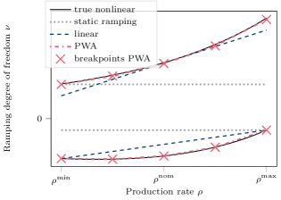
Figure 2: Constraints for ramping degree of freedom $\nu$ as function of production rate $\rho$. True nonlinear limits in comparison to static ramping limits, linear limits, and piece-wise affine (PWA) limits for an illustrative case with first-order dynamics. For first-order dynamics, the transformed state vector $\bm{\varphi}$ is of dimension one and equal to the production rate $\rho$. Consequently, the limits on the ramping degree of freedom $\nu$ only depend on $\rho$.

In general, the limits $\nu^{\text{min}}(\bm{\varphi})$, $\nu^{\text{max}}(\bm{\varphi})$ (Equations 27 and 28) are nonlinear functions and linear or piece-wise affine approximations are needed to achieve an MILP formulation. Fortunately, if both limits are approximated conservatively, the resulting trajectory is always feasible because the ramping degree of freedom $\nu$ stays within the true feasible range. In contrast to static ramping constraints, approximating the nonlinear limits allows to balance conservativeness against computational complexity as we discuss in the following for the case of first-order dynamics. If static ramping constraints or purely linear functions are chosen, computational costs are small. However, potentially, a high conservatism has to be accepted as a large amount of the feasible region for the ramping degree of freedom $\nu$ is cut off. In Figure 2, the feasible region between the nonlinear limits is much bigger than the feasible region between the static limits and also bigger than the feasible region between the linear limits. Using piece-wise affine functions, the conservative limits can enclose more of the feasible nonlinear region. However, if the feasible region is non-convex, binary variables have to be introduced, which significantly increase the computational burden in optimization.

In the case of first-order dynamics, the true limits on the ramping degree of freedom $\nu$ can simply be plotted to choose appropriate bounds. In case of high-order dynamics, the limits are multivariate functions and multivariate regression methods that give piece-wise affine functions, e.g., hinging hyperplanes (L. Breiman,, 1993; A. A. Adeniran and S. El Ferik,, 2017; Kämper et al.,, 2021), convex region surrogates (Zhang et al.,, 2016; Schweidtmann et al.,, 2021), or artificial neural networks with ReLU activation functions (Bjarne Grimstad and Henrik Andersson,, 2019), must be used. However, as discussed after Equation (4n+1), typically the number of necessary differentiations is expected to be small.

By employing a conservative approximation of the true nonlinear ramping limits, the feasibility of the found solution on the original nonlinear model is guaranteed. As feasible area is cut off, the found optimum of the approximated MILP problem might deviate from the optimal solution of the original MINLP problem, i.e., optimality on the original problem might not be achieved. However, with piecewise affine functions, the true nonlinear limits can, in principle, be approximated to any accuracy if a sufficient number of piecewise linear elements is used. These piecewise linear elements however can increase the number of binary variables leading to higher computational cost. Thus, a suitable trade-off between accuracy of the approximation and number of binary variables must be found.

4 Case Study

As case study, we consider two continuous stirred tank reactors (CSTRs) with different dynamic orders in parallel configuration. The first CSTR is a dimensionless benchmark CSTR from literature (Flores-Tlacuahuac and Grossmann,, 2006; Du et al.,, 2015) described by material and energy balances. Note that, for this CSTR, the material flow rate equals the production rate. As we use the symbol $\rho$ for the production rate throughout the paper, we denote the material flow rate as $\rho$ to preserve consistency, even if this is an unusual choice.

$$\dot{c}=(1-c)\frac{\rho}{V}-cke^{-\frac{N}{T}}$$ (CSTR1a)

$$\dot{T}=(T_{f}-T)\frac{\rho}{V}+cke^{-\frac{N}{T}}-F_{c}\alpha_{c}\left(T-T_{c}\right)$$ (CSTR1b)

The CSTR states $\mathbf{x}$ are the concentration $c$ and the temperature $T$. The control input $u$ is the coolant flow rate $F_{c}$ with bounds $F_{c}^{min}=0\frac{1}{h}$, $F_{c}^{max}=700\frac{1}{h}$ (Du et al.,, 2015). The material flow rate $\rho$ is a degree of freedom and equals the production rate. All other symbols are constant parameters given in Table 1. Following Schäfer et al., (2020), we assume an oversizing of 20 % such that the dimensionless production rate can be varied by +/- 20 % around the nominal value $\rho^{nom}=1\frac{1}{h}$, i.e., $\rho^{\text{min}}=0.8\frac{1}{h}$ and $\rho^{\text{max}}=1.2\frac{1}{h}$. Additionally, we assume that the concentration has to be maintained constant at $c=c^{nom}=0.1367$ (product 2 in Flores-Tlacuahuac and Grossmann, (2006)). Thus, the output $y$ is given by $y=h(\mathbf{x})=c$. The second CSTR is identical to the first CSTR except for an additional inertia in the form of a cooling jacket with temperature $T_{j}$. With an energy balance of the cooling jacket, the model of CSTR 2 reads:

Equation (CSTR1a) (CSTR2a)

$$\dot{T}=(T_{f}-T)\frac{\rho}{V}+cke^{-\frac{N}{T}}+\tau_{1}(T_{j}-T)$$ (CSTR2b)

$$\dot{T}_{j}=\tau_{2}(T-T_{j})-F_{c}\alpha_{c}\left(T_{j}-T_{c}\right)$$ (CSTR2c)

The inverse time constants $\tau_{1}$, $\tau_{2}$ are derived from the reactor studied in M. Mezghani et al., (2002) and given in Table 1.

Table 1: Dimensionless CSTR model parameters from Flores-Tlacuahuac and Grossmann, (2006); Du et al., (2015) and time constants from M. Mezghani et al., (2002).

	symbol	value
volume	$V$	$20$
reaction constant	$k$	$300\frac{1}{h}$
activation energy	$N$	5
feed temperature	$T_{f}$	0.3947
heat transfer coefficient	$\alpha_{c}$	$1.95\cdot 10^{-4}$
coolant temperature	$T_{c}$	0.3816
inverse time constant	$\tau_{1}$	$4.84\frac{1}{h}$
inverse time constant	$\tau_{2}$	$14.66\frac{1}{h}$

We study the two CSTRs in combination with a benchmark multi-energy system from Sass et al., (2020). The waste heat of the two flexible CSTRs is integrated to partly satisfy the heat demand of inflexible consumers (Figure 3). In other words: The two CSTRs demand cooling but the removed heat is integrated such that the CSTRs supply waste heat. The dimensionless waste heat $Q_{wh}$ is:

$$Q_{wh}=F_{c}\alpha_{c}\left(T-T_{c}\right)$$ (38)

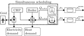
Figure 3: Case Study: Simultaneous scheduling of two continuous stirred tank reactors (CSTRs) with variable production rates $\rho_{1}$ and $\rho_{2}$, a boiler, and a combined heat and power plant (CHP). The waste heat of the two CSTRs, $Q_{wh1}$ and $Q_{wh2}$, is used to partly satisfy a non-flexible heat demand. Additionally, a non-flexible electricity demand has to be fulfilled.

The multi-energy system consists of a combined heat and power plant (CHP) and a boiler (Bo) that together need to satisfy a heat demand and an electricity demand. Electricity can be bought from the grid and sold to the grid. As the demands in Sass et al., (2020) (available online at HECI, (2021)) are calculated using weather data from the 28th November 2018, we use the German day-ahead market price series for electricity from the same day (SMARD Marktdaten,, 2021). We scale the waste heat of the dimensionless benchmark CSTRs such that the nominal waste heat of each CSTR corresponds to 10% of the maximum heat demand. Both CHP and boiler have a variable part-load efficiency and a minimum part-load (Sass et al.,, 2020).

4.1 Derivation of dynamic ramping constraints

The first CSTR has two differential states and is exactly input-state linearizable, i.e., the relative degree $r$ is 2. Thus, the output $y$ has to be differentiated two times until the input $u=F_{c}$ appears explicitly:

$$y= c\coloneqq\alpha_{0}(c)\overset{!}{=}c^{\text{nom}}$$ (39)

$$\dot{y}= \frac{\partial\alpha_{0}(c)}{\partial c}\dot{c}=(1-c)\frac{\rho}{V}-cke^{-\frac{N}{T}}\coloneqq\alpha_{1}(c,T,\rho)\overset{!}{=}0$$ (40)

$$y^{(2)}= \frac{\partial\alpha_{1}(c,T,\rho)}{\partial c}\dot{c}+\frac{\partial\alpha_{1}(c,T,\rho)}{\partial T}\dot{T}+\frac{\partial\alpha_{1}(c,T,\rho)}{\partial\rho}\dot{\rho}$$ (41)

$$= -\left[\frac{\rho}{V}+ke^{-\frac{N}{T}}\right]\left[(1-c)\frac{\rho}{V}-cke^{-\frac{N}{T}}\right]$$

$$-\left[\frac{ckNe^{-\frac{N}{T}}}{T^{2}}\right]\left[(T_{f}-T)\frac{\rho}{V}+cke^{-\frac{N}{T}}-F_{c}\alpha_{c}\left(T-T_{c}\right)\right]+\left[\frac{1-c}{V}\right]\dot{\rho}$$

$$= \alpha_{2}(\mathbf{x},\rho)+\beta_{u}(\mathbf{x},\rho)F_{c}+\beta_{\rho}(\mathbf{x},\rho)\nu\overset{!}{=}0,$$

$$\text{with }\nu=\dot{\rho},\leavevmode\nobreak\ \alpha_{2}(\mathbf{x},\rho)=-\left[\frac{\rho}{V}+ke^{-\frac{N}{T}}\right]\left[(1-c)\frac{\rho}{V}-cke^{-\frac{N}{T}}\right]$$

$$-\left[\frac{ckNe^{-\frac{N}{T}}}{T^{2}}\right]\left[(T_{f}-T)\frac{\rho}{V}+cke^{-\frac{N}{T}}\right],$$

$$\beta_{u}(\mathbf{x},\rho)=\frac{ckNe^{-\frac{N}{T}}\alpha_{c}\left(T-T_{c}\right)}{T^{2}}>0,\text{ and }\beta_{\rho}(\mathbf{x},\rho)=\frac{1-c}{V}>0$$

Consequently, the production rate $\rho$ can be changed with a first-order dynamic because only the first derivative of the production rate appears during the differentiations. The equation system to calculate the transformation $\mathbf{x}=\bm{\Gamma}(\rho)$ (compare to Equation (37)) is given by Equations (39) and (40). The determinant of the Jacobian is $-\frac{ckNe^{-\frac{N}{T}}}{T^{2}}$ (compare to discussion after Equation (37)), which is always nonzero as the states $c,T$ are always nonzero in the considered operating range, and the parameters $k,N$ are also nonzero. Consequently, the two equations can be solved to calculate the state vector $\mathbf{x}$ as function of the production rate $\rho$:

$$\underbrace{\left(\begin{array}[]{c}c\\ T\end{array}\right)}_{\mathbf{x}}=\underbrace{\left(\begin{array}[]{c}c^{nom}\\ \frac{N}{\ln{\left(\frac{Vck}{\rho\left(1-c\right)}\right)}}\end{array}\right)}_{\bm{\Gamma}(\rho)}$$ (46)

With $\bm{\Gamma}(\rho)$, the limits of the ramping degree of freedom $\nu$ are calculated as a function of the production rate $\rho$ using Equations (27) and (28) (Figure 4). Based on the visualization in Figure 4, we choose purely linear dynamic ramping limits $\nu^{\text{min}}(\rho)$, $\nu^{\text{max}}(\rho)$ as these give a good approximation. Note that in many control engineering applications, linear approximations give a reasonable approximation of nonlinear functions as long as the process is close to a nominal operating point (Corriou,, 2018) like in the example here.

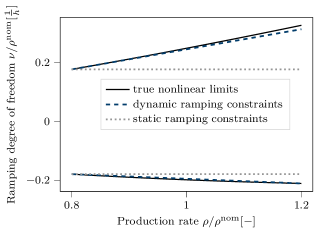
Figure 4: True nonlinear limits and linear dynamic ramping constraints for the non-jacketed CSTR 1. Static ramping constraints are indicated for comparison.

For the jacketed CSTR 2, the output $c$ must be differentiated three times until the input $u$ appears. For this CSTR, we only show the functional dependencies to avoid lengthy equations:

$$y =c\coloneqq\alpha_{0}(c)\overset{!}{=}c^{\text{nom}}$$ (47)

$$\dot{y} =\frac{\partial\alpha_{0}(c)}{\partial c}\dot{c}\coloneqq\alpha_{1}(c,T,\rho)\overset{!}{=}0$$ (48)

$$y^{(2)} =\frac{\partial\alpha_{1}(c,T,\rho)}{\partial c}\dot{c}+\frac{\partial\alpha_{1}(c,T,\rho)}{\partial T}\dot{T}+\frac{\partial\alpha_{1}(c,T,\rho)}{\partial\rho}\dot{\rho}\coloneqq\alpha_{2}(c,T,T_{j},\rho,\dot{\rho})\overset{!}{=}0$$ (49)

$$y^{(3)} =\frac{\partial\alpha_{2}(c,T,T_{j},\rho,\dot{\rho})}{\partial\mathbf{x}}\left(\begin{array}[]{c}\dot{c}\\ \dot{T}\\ \dot{T}_{j}\end{array}\right)+\frac{\partial\alpha_{2}(c,T,T_{j},\rho,\dot{\rho})}{\partial\bm{\varphi}}\left(\begin{array}[]{c}\dot{\rho}\\ \rho^{(2)}\end{array}\right)$$ (55)

$$=\alpha_{3}(\mathbf{x},\bm{\varphi})+\beta_{u}(\mathbf{x},\bm{\varphi})F_{c}+\beta_{\rho}(\mathbf{x},\bm{\varphi})\nu\overset{!}{=}0\text{ with }\nu=\rho^{(2)}$$

The complete derivatives are given in the Supplementary Information. For CSTR 2, the Jacobian of Equation (37) is $\frac{N^{2}\alpha_{c}c^{2}k^{2}e^{-\frac{2N}{T}}}{T^{4}}$, which is always nonzero. Thus, the states $\mathbf{x}$ can be given as a function of the ramping state vector $\bm{\Gamma}(\bm{\varphi})$. As the second time derivative of the production rate, $\rho^{(2)}$, appears in $y^{(3)}$, this second derivative $\rho^{(2)}$ is the ramping degree of freedom $\nu$ and the ramping state vector $\bm{\varphi}$ is two-dimensional $\bm{\varphi}=\left(\begin{array}[]{c}\rho\\ \dot{\rho}\end{array}\right)$. In other words: A second-order ramping constraint with $\delta=2$ in Equation DRCa is needed. We choose the simplified ramping limits $\nu^{\text{min}}(\rho,\dot{\rho})$, $\nu^{\text{max}}(\rho,\dot{\rho})$ to be linear in both $\rho$ and $\dot{\rho}$:

$$\nu^{\text{min}}(\rho,\dot{\rho})=\nu_{0}^{\text{min}}+m_{\rho}^{\text{min}}\rho+m_{\dot{\rho}}^{\text{min}}\dot{\rho}$$ (56)

$$\nu^{\text{max}}(\rho,\dot{\rho})=\nu_{0}^{\text{max}}+m_{\rho}^{\text{max}}\rho+m_{\dot{\rho}}^{\text{max}}\dot{\rho},$$ (57)

with parameters $\nu_{0}^{\text{min}}$, $m_{\rho}^{\text{min}}$, $m_{\dot{\rho}}^{\text{min}}$, $\nu_{0}^{\text{max}}$, $m_{\rho}^{\text{max}}$, $m_{\dot{\rho}}^{\text{max}}$. To parameterize the bounds, we sample the operating range using 100 equally distributed points for $\rho$ and 100 equally distributed points for $\dot{\rho}$ such that there are 10,000 points in total. For each point, the true nonlinear limits are calculated, and the parameters are fitted to the nonlinear limits using the normal equation method (Lewis et al.,, 2006). To make the resulting limits conservative, we search through the grid for the highest violation of the nonlinear limits and adapt $\nu_{0}^{\text{min}}$ and $\nu_{0}^{\text{max}}$ to the safe side. As visualized in Figure 5, again the linear limits are close to the nonlinear limits. This finding could be expected because linear limits already give a reasonable approximation for the non-jacketed CSTR1 and the additional heat transfer terms in Equations (CSTR2b) and (CSTR2c) are purely linear.

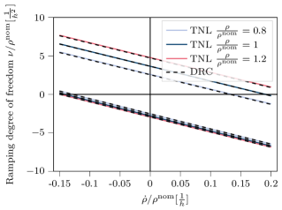
Figure 5: True nonlinear limits (TNL) and corresponding linear dynamic ramping constraints (DRC) for the jacketed CSTR 2. The limits are functions of the production rate $\rho$ and its first derivative $\dot{\rho}$. In this figure, the limits are given depending on $\dot{\rho}$ for 3 different values of $\rho$.

To illustrate the dynamic ramping constraints derived for the non-jacketed CSTR 1 and the jacketed CSTR 2, we perform a first optimization in which we ramp the reactors from minimum production rate to maximum production rate as fast as possible (Figure 6). For CSTR 1, the ramp up takes 1.7 h while it would take 2.3 h (+35 %) with a static ramping constraint where the maximum ramping $\nu^{\text{max}}$ is constant (Figure 4). The ramp up of the jacketed CSTR 2 takes more than half an hour longer compared to CSTR 1 because of the cooling jacket inertia. We cannot compare the ramp-up of CSTR 2 to traditional first-order static ramping because $y^{(3)}$ can only be held constant by manipulating $F_{c}$ if the second derivative of the production rate $\rho^{(2)}$ is defined (compare to Equation (55)). A first-order ramp would give a step change on the first derivative $\dot{\rho}$ such that $\rho^{(2)}$ is not defined and the output $y$ must deviate from the nominal value. Depending on the application, such deviations might be acceptable, still, they can be avoided using a second-order ramp. Moreover, if deviations are only acceptable up to a certain tolerance, it might be necessary to choose a first order ramp slow enough such that deviations can be corrected by the underlying control while a second-order ramp might allow a faster ramp-up.

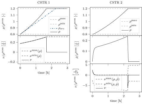
Figure 6: Fastest possible ramp up from minimum production rate $\rho^{\text{min}}$ to maximum production rate $\rho^{\text{max}}$ for CSTR 1 and CSTR 2. The ramping degree of freedom $\nu$ is shown together with its dynamic limits $\nu^{\text{min}}(\cdot)$, $\nu^{\text{max}}(\cdot)$. For CSTR 1, the fastest possible ramp up with a static ramping constraint $\rho_{src}$ is shown for comparison.

As linear dynamic ramping constraints are used for the two CSTRs, we expect the resulting formulation to be computationally efficient. Moreover, the two shortcomings of static ramping constraints can be illustrated: While the jacketed CSTR2 cannot be modeled accurately by static ramping constraints due to second-order dynamics, dynamic ramping constraints ramp up the non-jacketed CSTR1 35 % faster than static ramping constraints.

4.2 Waste heat model

For the dynamic MILP scheduling problem P2, a process energy demand model is needed (P2c). In this case study, the energy demand of the CSTRs corresponds to the waste heat removed from the CSTRs (cf. Figure 3). For the scheduling waste heat model, we start by investigating purely linear functions as approximation

$$Q_{wh1}=a_{0,1}+a_{1,1}\rho_{1}+a_{2,1}\nu_{1},$$ (58)

$$Q_{wh2}=a_{0,2}+a_{1,2}\rho_{2}+a_{2,2}\dot{\rho}_{2}+a_{3,2}\nu_{2},$$ (59)

with coefficients $a_{0,1}$, $a_{1,1}$, $a_{2,1}$, $a_{0,2}$, $a_{1,2}$, $a_{2,2}$, $a_{3,2}$. To determine the coefficients, we sample the operating region using 11 equally distributed points for $\rho$, $\nu$, and $\dot{\rho}$ (only CSTR2), which gives $11\times 11$ points for CSTR 1 and $11\times 11\times 11$ points for CSTR 2. For each point, we calculate the waste heat from the nonlinear model and subsequently fit the coefficients using the normal equation method (Lewis et al.,, 2006). The average absolute deviation between fit and nonlinear model is 4 % of the nominal waste heat for CSTR 1 and 1 % of the nominal waste heat for CSTR 2. As these deviations are small, we do not study potentially more accurate piece-wise affine models for the waste heat. Moreover, we assume that small deviations can be compensated by the energy system components, as these components typically react much faster than the chemical process.

4.3 Optimization problem

Based on the dynamic ramping constraints and the waste heat model, in this subsection, we formulate the scheduling optimization problem P2.

Following Voll, (2014), the efficiency curves (Equation (P1g)) for CHP and boiler specified in Sass et al., (2020) are discretized with one affine element to obtain a satisfactory discretization. Note that a small number of piece-wise affine elements, i.e., one or two, is often sufficient for modeling univariate efficiency functions of typical energy system components (Andreas Kämper et al.,, 2021).

For the storage units, we enforce that the filling level is 50 % of the maximum filling level at the beginning and the end of the day such that the total production is fixed. We assume that the capacity of the two storage units is equal to 3 hours of production at nominal production rate. A storage capacity of 3 hours is the lower bound of the range studied by Schäfer et al., (2020) who consider storage capacities between 3 and 48 hours for demand response applications. We find that the storage capacity is no limiting factor in our case study, i.e., the bounds of the storage filling level are never reached. Additionally, the optimization is repeated without storage constraints and the result does not change.

As electricity prices and energy demands are given with one hour time resolution, we use one hour timesteps for the ramping degrees of freedom $\nu_{1}$, $\nu_{2}$, and for the on/off binaries $z_{i}^{\text{on}}$ (cf. Equation P1h). The remaining variables are discretized with 2 collocation elements per hour and 4 points per element. Note that we calculate economic profit in a simulation and thereby automatically verify the adequacy of our time discretization.

The optimization problem is formulated using pyomo (Hart et al.,, 2017, 2011) and pyomo.dae (Nicholson et al.,, 2018) for discretization. We solve the optimization problem using gurobi version 8.1.0 (Gurobi Optimization, LLC,, 2021) with zero optimality gap. All calculations are performed on a Windows 10 machine with an Intel(R) Core(TM) i5-8250U core and 24 GB RAM.

4.4 Results

The cost reductions achieved by waste heat integration relate to an operation without waste heat integration. First, we calculate the cost reductions through waste heat integration in a scenario without DR, i.e., both CSTRs are operated in steady state such that waste heat production is constant. Second, in the DR scenario, we optimize the operation of energy system and CSTRs simultaneously, i.e., we solve the dynamic ramping problem (P2). Next, we simulate the resulting schedule on the original nonlinear process model over the 24 hour time horizon to determine the cost reduction achieved through waste heat integration. Third, to bound the DR potential, we solve the original MINLP problem (P1) using the solver BARON version 20.10.16 (Khajavirad and Sahinidis,, 2018). As BARON with default settings does not provide a feasible point after 2 hours of optimization, we generate a point by fixing the integer on/off-decisions to the values from the solution of our dynamic ramping problem (P2), i.e., we reduce the MINLP to a nonlinear program (NLP). For this NLP, BARON provides a feasible point, which we use as initial point to solve the original MINLP (P1) with BARON. After 2 hours of calculation, we use the reported lower bound to determine the maximum possible DR potential.

The DR scenario reduces 40.8 % more costs than the steady-state scenario (Table 2). This DR improvement is only slightly below the MINLP bound, which is 42.7 %. Further, the optimization runtime of the dynamic ramping problem (P2) is below 2 seconds, which is short enough for online application.

Table 2: Cost reduction for the considered day achieved by waste heat integration for different scenarios. For the MINLP solution the lower bound found after 2 hours of optimization is reported.

Scenario	Cost reduction [€]	DR improvement [%]
No DR (steady-state, operation)	90.11	-
DR with dynamic ramping (P2)	126.91	40.8
MINLP bound (P1)	128.61	42.7

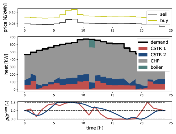
Figure 7: Resulting operation in the DR scenario with dynamic ramping constraints showing the heat supplied by the two CSTRs, the CHP, and the boiler, and the production $\rho$ delivered by the two CSTRs (in red for CSTR 1 and blue for CSTR 2).

Interestingly, in the DR scenario, the boiler is only active for 1 hour (Figure 7) while the boiler is active for 11 hours in the steady-state scenario. The reason is that for the given prices, the CHP is less expensive compared to the boiler. Thus, the main cost reduction is achieved by shifting waste heat in time such that the boiler can be turned off. This point is demonstrated by repeating the DR optimization but fixing the boilers on/off-decisions to the 11 hours of operation from the steady-state scenario. The cost reduction is only 95.3 €, i.e., instead of 40.8% improvement through DR only 5.7% is realized.

In our case study, the simultaneous scheduling of processes and multi-energy system provides significant cost reductions via DR. To realize the possible cost reductions, the discrete on/off-decisions in the multi-energy system need to be considered during optimization. Using our high-order dynamic ramping constraints, we achieve optimization runtimes that allow an online application while the economic result is only slightly worse compared to MINLP optimization.

4.5 Comparison with first-order static ramping constraints

Finally, we compare our high-order dynamic ramping constraints to first-order static ramping constraints. As discussed, first-order ramping constraints are not applicable to the jacketed CSTR2 and we thus focus on the non-jacketed CSTR 1. For CSTR1, the case study result does not change significantly if we use static instead of dynamic ramping constraints which is for two reasons: First, the difference between static and dynamic ramping constraints is small as we only vary the operating point by +/- 20% (Figure 4). Second, the optimal schedule shifts just enough waste heat in each time step such that the boiler can be turned off and thus the full ramping capabilities of CSTR 1 are not exploited. To demonstrate the benefits of dynamic ramping constraints more clearly, we expand the operating range to +/- 50 % such that the difference between dynamic and static ramping constraints becomes more pronounced (Figure 8). Further, to study the ramping of CSTR 1 decoupled from on/off decisions, we modify the case study setup such that it contains only CSTR1, a CHP, and a constant heat demand. All produced electricity is sold to the grid. Moreover, we use a price profile that exhibits low prices for several hours and thus motivates a long period of ramping down. The price profile occurred on the 24th February 2018 at the German day-ahead market (SMARD Marktdaten,, 2021).

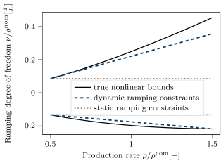
Figure 8: True nonlinear bounds, linear dynamic ramping constraints, and static ramping constraints for the non-jacketed CSTR 1 in the modified case study.

The DR improvement is 6.7% with static ramping constraints (SRC) while it becomes 12.2 % with dynamic ramping constraints (DRC) (Table 3), i.e., the dynamic ramping constraints nearly double the benefits of demand response. For static ramping constraints, the highest realized production rate is 133% of the nominal production rate and the minimal production rate is 58%. In contrast, the range is 150%-54% with dynamic ramping constraints. Especially, in the first two hours, the DRC scenario ramps up to 150% while the SRC scenario only reaches 117% (Figure 9). This faster ramping increases the DR improvement because the morning hours have cheap electricity prices, which make operation of the CHP unfavorable, and thus favor a high waste heat production. Most waste heat is produced when the reactor ramps down as the temperature needs to be lowered during down-ramping. While SRC ramp down starts from 117% production rate in hour 2, DRC ramp down starts from 150% production and therefore generates more waste heat. The modified case study demonstrates that in cases where fast ramping is required dynamic ramping constraints can significantly improve demand response compared to static ramping constraints.

Table 3: Cost reduction achieved by waste heat integration in modified case study.

Case	Cost reduction [€]	DR improvement [%]
No DR	81.1	-
DR with SRC	86.5	6.7
DR with DRC	91.0	12.2

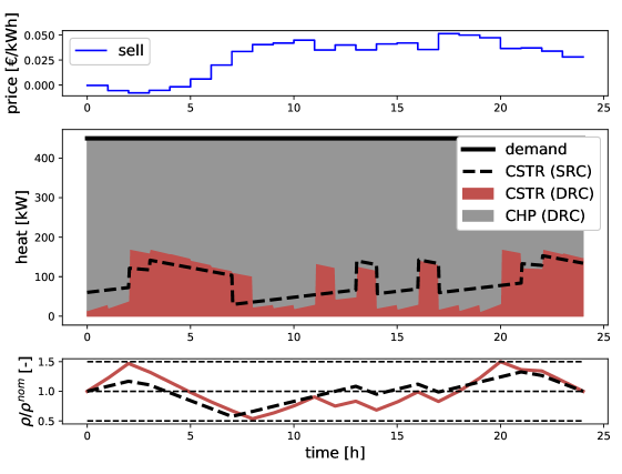
Figure 9: Resulting operation in the modified case study showing the heat supplied by CSTR and CHP, and the production $\rho$ delivered by the CSTR for the case of dynamic ramping constraints (DRC) (red line). For comparison, the waste heat and production rate with static ramping constraints (SRC) are shown as black dashed lines.

5 Discussion of possible extensions

In this section, we discuss four possible extensions of the dynamic ramping method, its integration with control, and the applicability of the approach.

Extension 1: In some cases, it might be favorable to vary the output $y$ with the production rate instead of holding it constant because varying the output gives additional flexibility for example to choose optimal steady-state operating points. The output can be varied if a function $\pi$ is chosen that defines the output $y$ as an $n$ times differentiable function of the production rate $\rho$. Consequently, the desired values of output $y$ and its time derivatives are (compare to Equations (4.1) - (4.n+1)):

$$y \overset{!}{=}\pi(\rho)$$ (60)

$$\dot{y} \overset{!}{=}\frac{\partial\pi(\rho)}{\partial\rho}\dot{\rho}$$ (61)

$$y^{(2)} \overset{!}{=}\frac{\partial^{2}\pi(\rho)}{\partial^{2}\rho}\dot{\rho}^{2}+\frac{\partial\pi(\rho)}{\partial\rho}\rho^{(2)}$$ (62)

$$\vdots$$

Still, the Equation system (37) is defined and our dynamic ramping reformulation can in principle be applied. Note that the equation system is more complex to solve if the output $y$ is not constant anymore.

Extension 2: Bounds on states are not considered in our example, however, they can be considered in a straightforward manner, as all states $\mathbf{x}$ are given as a function $\bm{\Gamma}(\bm{\varphi})$ of the ramping state vector $\bm{\varphi}$ (compare to Section 3.2). For example, for the jacketed CSTR 2, the jacket temperature $T_{j}$ is given as a function $\Gamma(\rho,\dot{\rho})$ of the production rate $\rho$ and its first derivative, $\dot{\rho}$. If the equation $T_{j}=\Gamma(\rho,\dot{\rho})$ can be solved for the derivative $\dot{\rho}$ to $\dot{\rho}=\Gamma^{-1}(\rho,T_{j})$, one can insert the bounds of the state $T_{j}$ into the function $\Gamma^{-1}$ and receive bounds on the derivative $\dot{\rho}$ as a function of the production rate $\rho$. Thus, bounds on the state $T_{j}$ can be considered by adding a first-order ramping constraint ($\dot{\rho}^{\text{min}}(\rho)\leq\dot{\rho}\leq\dot{\rho}^{\text{max}}(\dot{\rho})$).

Extension 3: As the presented derivation of dynamic ramping constraints is restricted to SISO processes, we continued to work on dynamic ramping constraints. We were able to generalize the rigorous derivation to flat MIMO processes (Baader et al., 2022a, ). Note that for SISO processes, flatness is equivalent to exact input-state linearizability, which we use in the current article. The derivation of dynamic ramping constraints for MIMO processes follows the same concept as for SISO processes and is similar to the current paper’s derivation.

Extension 4: Here, we only derive dynamic ramping constraints rigorously for the case that the relative degree $r$ equals the number of states $n$ ($r=n$). The case $r>n$ is not relevant as for $r>n$, the output $y$ is not controllable with the input $u$. For the case $r<n$, internal dynamics occur (Corriou,, 2018). Consequently, the process state is not fully described by $y$ and its first $r-1$ time derivatives but there are $n-r$ internal states. Such processes are called input-output linearizable (Corriou,, 2018). For input-output linearizable processes, our method would still allow to determine the order of dynamic ramping constraints rigorously. However, the limits $\nu^{\text{min}}$, $\nu^{\text{max}}$ varying with the operation point $\bm{\varphi}$ would additionally depend on the unknown internal states. Possibly, the internal states could be treated as bounded uncertainties and robust limits that hold for all possible values of the internal states could be calculated (Ben-Tal et al.,, 2009). Alternatively, internal states might be estimated based on the trajectory of $\bm{\varphi}$, similar to the estimation of unmeasured intrinsic states performed by Lovelett et al., (2020).

Integration with control: Our scheduling with dynamic ramping constraints can be combined with any regulatory control. The result of the scheduling is a trajectory for the production rate $\rho$. Due to the derivation of dynamic ramping constraints, it is guaranteed that if the trajectory of the production rate is applied to the process, the regulatory control can choose a feasible input $u$ ( $u^{\text{min}}\leq u\leq u^{\text{max}}$) that keeps the output $y$ at its nominal value (compare to Section 3.2). However, if the scheduling decision is to ramp the production rate of the process as fast as possible, the input $u$ will be at its bound. If in such a situation the controlled output $y$ deviates from its nominal value due to disturbances, noise, or model-plant mismatch, the control might be unable react as the input $u$ is already at its bound. Thus, a deviation of the output $y$ from its nominal value must be tolerated. To solve this problem, the derivations of dynamic ramping constraints can be adapted to maintain the input within $u^{\text{min}}-\Delta u^{\text{control}}\leq u\leq u^{\text{max}}-\Delta u^{\text{control}}$, with a safety margin $\Delta u^{\text{control}}$ that the regulatory control can use to compensate for disturbances.

Even though any regulatory control can be used in principle, a feedforward linearization control structure (Hagenmeyer and Delaleau, 2003a, ; Hagenmeyer and Delaleau, 2003b, ) is particularly promising as the feedforward part simplifies the task for the regulatory control. That is, the nominal control input $u^{\text{nom}}$ needed to reject the disturbances introduced by varying the production rate is calculated using Equation (4.n+1) and directly applied to the process such that the underlying control does not have to compensate for the disturbance by the production rate anymore. To reject other disturbances that might act on the process, a simple tracking controller, e.g., a PID-controller, is added to stabilize the feedforward control (Hagenmeyer and Delaleau, 2003a, ; Hagenmeyer and Delaleau, 2003b, ).

Overall, the applicability of our method is strongly limited due to the strict assumptions. Still, as our results show that the dynamic ramping method could bridge the gap between nonlinear process models and simplified process representations for real-time scheduling, further research regarding the discussed extensions seems promising. Additionally, we argue that the number of scheduling-relevant dynamics is typically small (Du et al.,, 2015; Baldea and Harjunkoski,, 2014). Consequently, even if the mechanistic process model under consideration might not fulfill our assumptions, it might be possible to consider a reduced-order model for the slow scheduling relevant dynamics to which dynamic ramping constraints can be applied. For example, detailed electrolyzer models are typical MIMO models with several dynamics (Hoffmann et al.,, 2021). However, typically, only the slow temperature dynamic has to be considered on the hourly time scale relevant for demand response (Simkoff and Baldea,, 2020; Flamm et al.,, 2021). In a recent conference publication, we show that dynamic ramping constraints can be transferred to electrolyzers with slow temperature dynamics and increase demand response potential compared to quasi-steady-state scheduling (Baader et al., 2022b, ).

6 Conclusion

In this paper, we propose high-order dynamic ramping constraints for the simultaneous demand response (DR) optimization of processes and their multi-energy systems. These dynamic ramping constraints can be of high order and the ramping limits depend on the process state. Process-state-dependent limits enable faster transitions than typical static ramping constraints. Based on the notion of exact linearization, we derive dynamic ramping constraints rigorously for the case of exact input-state linearizable single-input single-output (SISO) processes.

In a case study, we consider two continuous stirred-tank reactors (CSTRs) with waste heat integration that are scheduled simultaneously with a multi-energy system. Deriving dynamic ramping constraints from the two CSTR models, we formulate an MILP optimization problem and improve the economic value of the waste heat by 41 % compared to steady-state operation. This benefit is close to the bound of 43% obtained from nonlinear mixed-integer dynamic optimization (MIDO) with the original process model. Importantly, the MILP formulation based on dynamic ramping constraints allows to solve the simultaneous DR optimization within seconds.

In a modified case study, we find that the DR improvement with dynamic ramping constraints is significantly higher than that with static ramping as the state-dependent ramping limits allow faster ramping. Consequently, the proposed high-order dynamic ramping constraints allow to capture the dynamic flexibility of processes better than traditional ramping constraints and achieve optimization runtimes sufficiently fast for online optimization.

Author contributions

Florian J. Baader: Conceptualization, Methodology, Software, Investigation, Validation, Visualization, Writing - original draft. Philipp Althaus: Conceptualization, Writing – review & editing. André Bardow: Funding acquisition, Conceptualization, Supervision, Writing – review & editing. Manuel Dahmen: Conceptualization, Supervision, Writing – review & editing.

Declaration of Competing Interest

We have no conflict of interest.

Nomenclature

Abbreviations
CSTR continuous stirred tank reactors DR demand response DRC dynamic ramping constraint MIDO mixed-integer dynamic optimization MILP mixed-integer linear program MIMO multi-input multi-output MINLP mixed-integer nonlinear program NLP nonlinear program SISO single-input single-output SRC static ramping constraint

Greek symbols
$\alpha$ nonlinear function $\alpha_{c}$ heat transfer coefficient $\beta$ nonlinear function $\Gamma$ state transformation $\delta$ order of DRC $\eta$ efficiency $\nu$ ramping degree of freedom $\rho$ production rate $\Phi$ objective $\tau$ time constant $\bm{\varphi}$ ramping state vector $\chi$ optimization variable

Latin symbols
$a$ fitting coefficient $c$ concentration $F$ flow rate $f$ nonlinear function $g$ nonlinear function $h$ nonlinear function $\mathbf{J}$ Jacobian matrix $k$ preexponential factor $N$ scaled activation energy $n$ number of states $p$ price $Q$ heat flow $r$ relative degree $S$ storage filling level $T$ temperature $t$ time $u$ input $V$ volume $x$ differential state $y$ output $z$ discrete variable

Sets
$\mathbb{C}$ energy system components $\mathbb{C}_{e}^{\text{cons}}$ energy system components that consume $e$ $\mathbb{C}_{e}^{\text{sup}}$ energy system components that supply $e$ $\mathbb{E}$ end energy forms

Subscripts
0 initial value $c$ cooling dem demand $e$ energy form $f$ feed $i$ energy system component $j$ jacket $m$ linear slope $src$ static ramping constraint $wh$ waste heat

Superscripts
$l$ lower bound max maximum value min minimum value nom nominal value $u$ upper bound

Bibliography

- A. A. Adeniran and S. El Ferik, (2017) A. A. Adeniran and S. El Ferik (2017). Modeling and identification of nonlinear systems: A review of the multimodel approach—part 1. IEEE Transactions on Systems, Man, and Cybernetics: Systems, 47(7):1149–1159.
- Agha et al., (2010) Agha, M. H., Thery, R., Hetreux, G., Hait, A., and Le Lann, J. M. (2010). Integrated production and utility system approach for optimizing industrial unit operations. Energy, 35(2):611–627.
- Andreas Kämper et al., (2021) Andreas Kämper, Ludger Leenders, Björn Bahl, and André Bardow (2021). Automog: Automated data-driven model generation of multi-energy systems using piecewise-linear regression. Computers & Chemical Engineering, 145:107162.
- (4) Baader, F. J., Althaus, P., Bardow, A., and Dahmen, M. (2022a). Demand response for flat nonlinear mimo processes using dynamic ramping constraints. arXiv:2205.14598.
- (5) Baader, F. J., Bardow, A., and Dahmen, M. (2022b). MILP formulation for dynamic demand response of electrolyzers. In Yamashita, Y. and Kano, M., editors, 14th International Symposium on Process Systems Engineering (PSE 2021+).
- (6) Baader, F. J., Bardow, A., and Dahmen, M. (2022c). Simultaneous mixed-integer dynamic scheduling of processes and their energy systems. AIChE Journal, page e17741.
- Baldea and Daoutidis, (2012) Baldea, M. and Daoutidis, P. (2012). Dynamics and Nonlinear Control of Integrated Process Systems. Cambridge Series in Chemical Engineering. Cambridge University Press.
- Baldea and Harjunkoski, (2014) Baldea, M. and Harjunkoski, I. (2014). Integrated production scheduling and process control: A systematic review. Computers & Chemical Engineering, 71:377–390.
- Ben-Tal et al., (2009) Ben-Tal, A., Nemirovskiĭ, A. S., and El Ghaoui, L. (2009). Robust optimization. Princeton series in applied mathematics. Princeton University Press, Princeton.
- Biegler, (2010) Biegler, L. T. (2010). Nonlinear Programming: Concepts, Algorithms, and Applications to Chemical Processes. Society for Industrial and Applied Mathematics.
- Bjarne Grimstad and Henrik Andersson, (2019) Bjarne Grimstad and Henrik Andersson (2019). Relu networks as surrogate models in mixed-integer linear programs. Computers & Chemical Engineering, 131:106580.
- Brée et al., (2019) Brée, L. C., Perrey, K., Bulan, A., and Mitsos, A. (2019). Demand side management and operational mode switching in chlorine production. AIChE Journal, 65(7):e16352.
- C. M. Correa-Posada et al., (2017) C. M. Correa-Posada, G. Morales-España, P. Dueñas, and P. Sánchez-Martín (2017). Dynamic ramping model including intraperiod ramp-rate changes in unit commitment. IEEE Transactions on Sustainable Energy, 8(1):43–50.
- Carrion and Arroyo, (2006) Carrion, M. and Arroyo, J. M. (2006). A computationally efficient mixed-integer linear formulation for the thermal unit commitment problem. IEEE Transactions on Power Systems, 21(3):1371–1378.
- Caspari et al., (2019) Caspari, A., Offermanns, C., Schäfer, P., Mhamdi, A., and Mitsos, A. (2019). A flexible air separation process: 2. optimal operation using economic model predictive control. AIChE Journal, pages 45–4393.
- Corriou, (2018) Corriou, J.-P. (2018). Process control: Theory and applications. Springer, Cham, Switzerland, second edition edition.
- Daoutidis et al., (2018) Daoutidis, P., Lee, J. H., Harjunkoski, I., Skogestad, S., Baldea, M., and Georgakis, C. (2018). Integrating operations and control: A perspective and roadmap for future research. Computers & Chemical Engineering, 115:179–184.
- Du et al., (2015) Du, J., Park, J., Harjunkoski, I., and Baldea, M. (2015). A time scale-bridging approach for integrating production scheduling and process control. Computers & Chemical Engineering, 79:59–69.
- Flamm et al., (2021) Flamm, B., Peter, C., Büchi, F. N., and Lygeros, J. (2021). Electrolyzer modeling and real-time control for optimized production of hydrogen gas. Applied Energy, 281:116031.
- Flores-Tlacuahuac and Grossmann, (2006) Flores-Tlacuahuac, A. and Grossmann, I. E. (2006). Simultaneous cyclic scheduling and control of a multiproduct cstr. Industrial & Engineering Chemistry Research, 45(20):6698–6712.
- Gurobi Optimization, LLC, (2021) Gurobi Optimization, LLC (2021). Gurobi optimizer reference manual. http://www.gurobi.com (accessed 10 October 2021).
- (22) Hagenmeyer, V. and Delaleau, E. (2003a). Exact feedforward linearization based on differential flatness. International Journal of Control, 76(6):537–556.
- (23) Hagenmeyer, V. and Delaleau, E. (2003b). Robustness analysis of exact feedforward linearization based on differential flatness. Automatica, 39(11):1941–1946.
- Hart et al., (2017) Hart, W. E., Laird, C. D., Watson, J.-P., Woodruff, D. L., Hackebeil, G. A., Nicholson, B. L., and Siirola, J. D. (2017). Pyomo–Optimization modeling in Python, volume 67. Springer Science & Business Media, second edition.
- Hart et al., (2011) Hart, W. E., Watson, J.-P., and Woodruff, D. L. (2011). Pyomo: Modeling and solving mathematical programs in python. Mathematical Programming Computation, 3(3):219–260.
- HECI, (2021) HECI (2021). https://jugit.fz-juelich.de/heci/energy-benchmark (accessed 13 October 2021).
- Hoffmann et al., (2021) Hoffmann, C., Hübner, J., Klaucke, F., Milojević, N., Müller, R., Neumann, M., Weigert, J., Esche, E., Hofmann, M., Repke, J.-U., Schomäcker, R., Strasser, P., and Tsatsaronis, G. (2021). Assessing the realizable flexibility potential of electrochemical processes. Industrial & Engineering Chemistry Research, 60(37):13637–13660.
- Iiro Harjunkoski et al., (2014) Iiro Harjunkoski, Christos T. Maravelias, Peter Bongers, Pedro M. Castro, Sebastian Engell, Ignacio E. Grossmann, John Hooker, Carlos Méndez, Guido Sand, and John Wassick (2014). Scope for industrial applications of production scheduling models and solution methods. Computers & Chemical Engineering, 62:161–193.
- Isidori, (1995) Isidori, A. (1995). Nonlinear Control Systems. Springer-Verlag London.
- Kämper et al., (2021) Kämper, A., Holtwerth, A., Leenders, L., and Bardow, A. (2021). Automog 3d: Automated data-driven model generation of multi-energy systems using hinging hyperplanes. Frontiers in Energy Research, 9:430.
- Khajavirad and Sahinidis, (2018) Khajavirad, A. and Sahinidis, N. V. (2018). A hybrid lp/nlp paradigm for global optimization relaxations. Mathematical Programming Computation, 10(3):383–421.
- L. Breiman, (1993) L. Breiman (1993). Hinging hyperplanes for regression, classification, and function approximation. IEEE Transactions on Information Theory, 39(3):999–1013.
- Leenders et al., (2019) Leenders, L., Bahl, B., Hennen, M., and Bardow, A. (2019). Coordinating scheduling of production and utility system using a stackelberg game. Energy, 175:1283–1295.
- Lewis et al., (2006) Lewis, J. M., Lakshmivarahan, S., and Dhall, S. (2006). Linear least squares estimation: Method of normal equations. In Dynamic Data Assimilation: A Least Squares Approach, Encyclopedia of Mathematics and its Applications, pages 99–120. Cambridge University Press.
- Lovelett et al., (2020) Lovelett, R. J., Avalos, J. L., and Kevrekidis, I. G. (2020). Partial observations and conservation laws: Gray-box modeling in biotechnology and optogenetics. Industrial & Engineering Chemistry Research, 59(6):2611–2620.
- M. Mezghani et al., (2002) M. Mezghani, G. Roux, M. Cabassud, M. V. Le Lann, B. Dahhou, and G. Casamatta (2002). Application of iterative learning control to an exothermic semibatch chemical reactor. IEEE Transactions on Control Systems Technology, 10(6):822–834.
- Merkert et al., (2015) Merkert, L., Harjunkoski, I., Isaksson, A., Säynevirta, S., Saarela, A., and Sand, G. (2015). Scheduling and energy – industrial challenges and opportunities. Computers & Chemical Engineering, 72:183–198.
- Meurer et al., (2017) Meurer, A., Smith, C. P., Paprocki, M., Čertík, O., Kirpichev, S. B., Rocklin, M., Kumar, A., Ivanov, S., Moore, J. K., Singh, S., Rathnayake, T., Vig, S., Granger, B. E., Muller, R. P., Bonazzi, F., Gupta, H., Vats, S., Johansson, F., Pedregosa, F., Curry, M. J., Terrel, A. R., Roučka, Š., Saboo, A., Fernando, I., Kulal, S., Cimrman, R., and Scopatz, A. (2017). SymPy: symbolic computing in Python. PeerJ Comput. Sci., page e103.
- Mitra et al., (2013) Mitra, S., Sun, L., and Grossmann, I. E. (2013). Optimal scheduling of industrial combined heat and power plants under time-sensitive electricity prices. Energy, 54:194–211.
- Mitsos et al., (2018) Mitsos, A., Asprion, N., Floudas, C. A., Bortz, M., Baldea, M., Bonvin, D., Caspari, A., and Schäfer, P. (2018). Challenges in process optimization for new feedstocks and energy sources. Computers & Chemical Engineering, 113:209–221.
- Nicholson et al., (2018) Nicholson, B., Siirola, J. D., Watson, J.-P., Zavala, V. M., and Biegler, L. T. (2018). Pyomo.dae: A modeling and automatic discretization framework for optimization with differential and algebraic equations. Mathematical Programming Computation, 10(2):187–223.
- Otashu and Baldea, (2019) Otashu, J. I. and Baldea, M. (2019). Demand response-oriented dynamic modeling and operational optimization of membrane-based chlor-alkali plants. Computers & Chemical Engineering, 121:396–408.
- Pattison et al., (2016) Pattison, R. C., Touretzky, C. R., Johansson, T., Harjunkoski, I., and Baldea, M. (2016). Optimal process operations in fast-changing electricity markets: Framework for scheduling with low-order dynamic models and an air separation application. Industrial & Engineering Chemistry Research, 55(16):4562–4584.
- Risbeck et al., (2017) Risbeck, M. J., Maravelias, C. T., Rawlings, J. B., and Turney, R. D. (2017). A mixed-integer linear programming model for real-time cost optimization of building heating, ventilation, and air conditioning equipment. Energy and Buildings, 142:220–235.
- Sass et al., (2020) Sass, S., Faulwasser, T., Hollermann, D. E., Kappatou, C. D., Sauer, D., Schütz, T., Shu, D. Y., Bardow, A., Gröll, L., Hagenmeyer, V., Müller, D., and Mitsos, A. (2020). Model compendium, data, and optimization benchmarks for sector-coupled energy systems. Computers & Chemical Engineering, 135:106760.
- Schweidtmann et al., (2021) Schweidtmann, A. M., Weber, J. M., Wende, C., Netze, L., and Mitsos, A. (2021). Obey validity limits of data-driven models through topological data analysis and one-class classification. Optimization and Engineering.
- Schäfer et al., (2020) Schäfer, P., Daun, T. M., and Mitsos, A. (2020). Do investments in flexibility enhance sustainability? a simulative study considering the german electricity sector. AIChE Journal, 66(11):e17010.
- Simkoff and Baldea, (2020) Simkoff, J. M. and Baldea, M. (2020). Stochastic scheduling and control using data-driven nonlinear dynamic models: application to demand response operation of a chlor-alkali plant. Industrial & Engineering Chemistry Research.
- Skogestad and Postlethwaite, (2001) Skogestad, S. and Postlethwaite, I. (2001). Multivariable Feedback Control: Analysis and Design. John Wiley & Sons, New York, USA, second edition edition.
- Slotine and Li, (1991) Slotine, J.-J. E. and Li, W. (1991). Applied nonlinear control. Prentice Hall.
- SMARD Marktdaten, (2021) SMARD Marktdaten (2021). https://www.smard.de/home/marktdaten (accessed 13 October 2021).
- T. Li and M. Shahidehpour, (2007) T. Li and M. Shahidehpour (2007). Dynamic ramping in unit commitment. IEEE Transactions on Power Systems, 22(3):1379–1381.
- Voll, (2014) Voll, P. (2014). Automated optimization-based synthesis of distributed energy supply systems. PhD thesis, RWTH Aachen University.
- Voll et al., (2013) Voll, P., Klaffke, C., Hennen, M., and Bardow, A. (2013). Automated superstructure-based synthesis and optimization of distributed energy supply systems. Energy, 50:374–388.
- Zhang and Grossmann, (2016) Zhang, Q. and Grossmann, I. E. (2016). Planning and scheduling for industrial demand side management: Advances and challenges. In Martín, M. M., editor, Alternative Energy Sources and Technologies, Engineering, pages 383–414. Springer, Switzerland.
- Zhang et al., (2016) Zhang, Q., Grossmann, I. E., Sundaramoorthy, A., and Pinto, J. M. (2016). Data-driven construction of convex region surrogate models. Optimization and Engineering, 17(2):289–332.