Anti-jamming beam alignment in millimeter-wave MIMO systems

Abstract

In millimeter-wave (MMW) multiple-input multiple-output (MIMO) communications, users and their corresponding base station (BS) have to align their beam during both initial access and data transmissions to compensate for the high propagation loss. The beam alignment (BA) procedure specified for 5th Generation (5G) New Radio (NR) has been designed to be fast and precise in the presence of non-malicious interference and noise. A smart jammer might exploit this weakness and may launch an attack during the BA phase in order to degrade the accuracy of beam selection and, thus, adversely impacting the end-to-end performance and quality-of-service experienced by the users. In this paper, we study the effects of a jamming attack at MMW frequencies during the BA procedure used to perform initial access for idle users and adaptation/recovery for connected users. We show that the BA procedure adopted in 5G NR is extremely vulnerable to a smart jamming attack and, consequently, we propose a countermeasure based on the idea of randomized probing, which consists of randomly corrupting the probing sequence transmitted by the BS in order to reject the jamming signal at the UE via a subspace-based technique based on orthogonal projections and jamming cancellation. Numerical results corroborate our theoretical findings and show the very satisfactory accuracy of the proposed anti-jamming approach.

I Introduction

The evolution of wireless radio-frequency (RF) communications has been basically driven by the unremitting pursuit of large portions of unexplored spectrum to boost the available data rates as much as possible. Unlike Long Term Evolution (LTE) systems, which mainly work below 3 GHz, 5th Generation (5G) New Radio (NR) are allowed to also operate in the millimeter-wave (MMW) band, with operating frequency from $24250$ MHz to $52600$ MHz [1, 2]. However, MMW communications are power-limited, because of higher path losses and blockage phenomena [3], which demand a significant technical breakthrough over the LTE system. Beamforming techniques are the standard way to provide the necessary signal-to-noise ratio (SNR) gain and provide spatial multiplexing, by using highly-directional beams [4, 5], especially in local coverage scenarios. Directional links are realized by antenna arrays with a large number of elements, which are feasible at MMW signaling since, due to the small wavelength, it is possible to package a large number of antenna elements at both the base station (BS) side and the user equipment (UE) side, implementing a massive multiple-input multiple-output (MIMO) system. All the lower layer functions are designed in NR on the basis of a beam-centric philosophy: in particular, unlike LTE, not only the user-plane channels, but also the control-plane channels are beamformed.

A problem arising in directional communications is how to establish, track and possibly reconfigure beams as the UE moves, or even when the UE device is simply rotated. Due to mobility and blockage, the current beam pair between the BS and UE may be blocked, resulting in a beam failure event. Beam failure could lead to radio link failure (RLF) already defined in LTE, which is managed by a costly higher-layer reconnection procedure. To deal with this issue, a new set of procedures, collectively referred to as beam alignment (BA) techniques, have been introduced in NR specifications, aimed at supporting possible fast beam reconfiguration and tracking, preferably working at the layers $1-2$ of the protocol stack. The beam-centric design is a groundbreaking difference between LTE and NR, which makes BA strategic for control and performance of MMW networks. Hence, with a widespread adoption of 5G NR, it is not difficult to imagine that BA will become the target of all kinds of potential threats or attacks.

I-A Deficiency of existing beam alignment procedure

The task of beam management is to acquire and maintain a reliable beam pair, i.e., a transmit angle-of-departure (AoD) and a corresponding receive angle-of-arrival (AoA) that jointly provides the best radio connectivity. The beam management procedures specified by the 3rd Generation Partnership Project (3GPP) in [6] and the subsequent works [7, 8, 9, 10, 11, 12, 13, 14, 15, 16, 17, 18, 19, 20, 21, 22, 23, 24, 25] are designed to be resilient to beam failure events due to mobility and blockage only. A noticible exception is represented by [26], where the beam training duration, training power, and data transmission power are optimized to maximize the throughput between two legitimate nodes, while ensuring a covertness constraint at a third-part node that attempts to detect the existence of the communication.

One serious threat to MMW network is the jamming attack during the BA phase, for which a jammer may transmit high-power RF signals to induce a beam failure event and, thus, a RLF that prevents either idle users from accessing the network or connected users from reconfiguration and tracking. Jamming attacks might dramatically increase the occurrence frequency of RLFs, thus lowering the quality of service of users and increasing costs for system management. To the best of our knowledge, the jamming attack specifically targeting at MMW links has not been considered yet and the synthesis of effective anti-jamming schemes is an open problem.

I-B Contribution and organization

Although other solutions are possible [6, 12], we focus in this paper on mobile-controlled BA (MCBA) [11] to perform initial access for idle users and adaptation/recovery for connected users, which can be summarized as follows:

• Beam sweeping: while all UEs stay in listening mode, the BS actively probes the channel by periodically broadcasting a beamforming codebook and a probing sequence over reserved beacon slots in the downlink.

• Beam measurement: the UE measures the quality of the received beamformed signals by using the received power or more sophisticated metrics, such as the SNR.

• Beam determination: the UE locally and independently identify the best beam.

• Beam reporting: the UE reports information regarding the best beam for successive data/control transmission or possible beam refinement over a control uplink channel.

MCBA is highly scalable and its overhead and complexity do not grow with the number of active users in the system. In this paper, due to the rapid development of software-defined radio techniques, we explicitly account for the presence of a smart jammer that is able to mimic the BS signal, which is formed by the transmit beamforming codebook and probing symbols.

Our study includes the main peculiar features of MMW networks. Specifically, according to NR physical-layer specifications, we consider orthogonal frequency-division multiplexing (OFDM) with cyclic prefix (CP) as a modulation format. Moreover, we exploit the fact that, at MMW frequencies, propagation in dense-urban non-line-of-sight (NLOS) environments is only based on a few scattering clusters, with relatively little delay/angle spreading within each cluster [27]. In this case, the MMW channel tends to exhibit a sparse structure in both angle and delay domains, which can be conveniently exploited to obtain anti-jamming alignment solutions. Finally, due to implementation/cost constraints of fully-digital architectures, we rely on a realistic MMW transmit implementation [28], according to which the number of RF chains is strictly smaller than the number of antennas. Within such a framework, our contributions are the following ones:

1. We develop a detailed model of a smart jamming attack in MMW networks, which represents an important, yet open research problem. The novelty of the proposed modeling approach rests mainly on the application to BA of jamming transmission techniques, which previous works attribute to communications based on centimetre-wave (CMW) communications [29].

2. Existing beam sweeping procedures [6, 7, 8, 9, 10, 11, 12, 13, 14, 15, 16, 17, 18, 19, 20, 21, 22, 23, 24, 25] rely on a publicly known protocol where the probing symbols are known to all UEs. As a countermeasure against the jamming attack, we propose the idea of randomized probing, which consists of superimposing a random sequence on the known probing symbols transmitted by the BS during the beam-sweeping phase. Such a random sequence is unknown to both the user and the jammer, but its subspace properties can be exploited at the UE to reject the contribution of the jamming signal. The idea of randomly corrupting the input data during the transmission has been used in other contexts with different aims, such as, to decentralize the transmission of a space time code from a set of distributed relays [30], to boost the performance or efficiency of neural networks [31], or to overcome the problem of pilot spoofing in CMW cellular systems [32].

3. Performance of the proposed anti-jamming methods are validated using a number of system parameters. It is demonstrated that a smart jamming attack leads to frequent beam failure events if no adequate countermeasures are taken. On the other hand, exploitation at the UE of randomized probing avoids beam misalignment, in such a way that costly beam recovery procedures are avoided while using lower-layer signaling.

The paper is organized as follows. The system model of the BA phase under a jamming attack is described in Section II. The study of the adverse effects of the jamming attack on a conventional BA algorithm is reported in Section III. The proposed countermeasure based on randomized probing is developed in Section IV. Numerical results are reported in Section V. Finally, conclusions are drawn in Section VI.

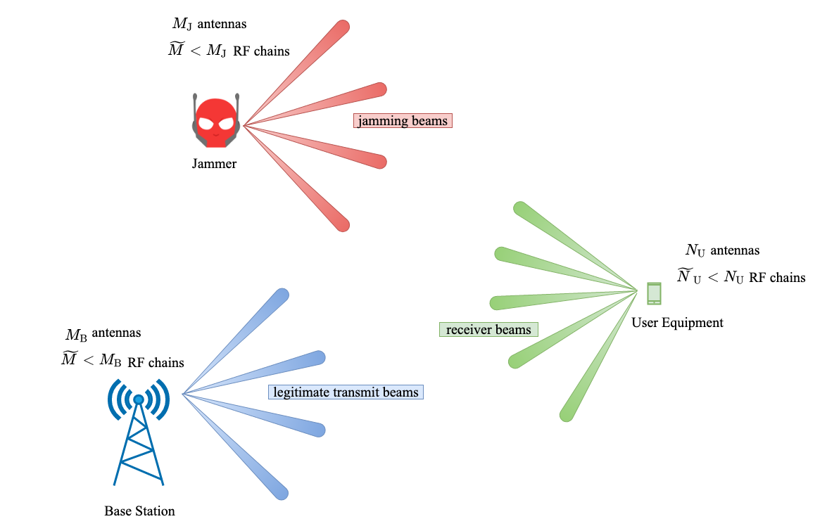
Figure 1: The jamming attack on the BA procedure in MMW MIMO systems.

I-C Notations

Upper- and lower-case bold letters denote matrices and vectors; the superscripts $*$, T, H, and $-1$ denote the conjugate, the transpose, the Hermitian (conjugate transpose), and the inverse of a matrix; $\mathbb{C}$, $\mathbb{R}$, $\mathbb{Z}$, and $\mathbb{N}$ are the fields of complex, real, integer, and natural numbers; $\mathbb{C}^{n}$ $[\mathbb{R}^{n}]$ denotes the vector-space of all $n$-column vectors with complex [real] coordinates; similarly, $\mathbb{C}^{n\times m}$ $[\mathbb{R}^{n\times m}]$ denotes the vector-space of all the $n\times m$ matrices with complex [real] elements; $\delta(\tau)$ is the Dirac delta; $\delta_{n}$ is the Kronecker delta, i.e., $\delta_{n}=1$ when $n=0$ and zero otherwise; $\jmath\triangleq\sqrt{-1}$ denotes the imaginary unit; $\text{max}(x,y)$ returns the maximum between $x\in\mathbb{R}$ and $y\in\mathbb{R}$; $\lceil x\rceil$ rounds $x\in\mathbb{R}$ to the nearest integer greater than or equal to $x$; the (linear) convolution operator is denoted with $\ast$; $\otimes$ stands for the Kronecker product; $|\mathcal{A}|$ is the cardinality of the set $\mathcal{A}$; $\mathbf{0}_{n}$, ${\mathbf{O}}_{n\times m}$ and ${\mathbf{I}}_{n}$ denote the $n$-column zero vector, the $n\times m$ zero matrix and the $n\times n$ identity matrix; ${\mathbf{x}}\geq{\mathbf{0}}_{n}$ [${\mathbf{x}}>{\mathbf{0}}_{n}$] denotes a vector ${\mathbf{x}}\in\mathbb{R}^{n}$ with non-negative [positive] entries; ${\mathbf{W}}_{n}\in\mathbb{C}^{n\times n}$ is the unitary symmetric $n$-point inverse discrete Fourier transform (IDFT) matrix, whose $(m+1,p+1)$-th entry is given by $\frac{1}{\sqrt{n}}\,e^{\jmath\frac{2\pi}{n}mp}$ for $m,p\in\{0,1,\ldots,n-1\}$, and its inverse ${\mathbf{W}}_{n}^{-1}={\mathbf{W}}_{n}^{\text{H}}$ is the $n$-point discrete Fourier transform (DFT) matrix; $\{\mathbf{a}\}_{\ell}$ is the $\ell$-th entry of ${\mathbf{a}}\in\mathbb{C}^{n}$, for $\ell\in\{1,2,\ldots,n\}$; $\{\mathbf{A}\}_{\ell_{1},\ell_{2}}$ is the $(\ell_{1},\ell_{2})$-th entry of ${\mathbf{A}}\in\mathbb{C}^{n\times m}$, for $\ell_{1}\in\{1,2,\ldots,n\}$ and $\ell_{2}\in\{1,2,\ldots,m\}$; matrix $\mathbf{A}={\text{diag}}(a_{0},a_{1},\ldots,a_{n-1})\in\mathbb{C}^{n\times n}$ is diagonal; vector $\mathbf{a}={\text{vec}}(\mathbf{A})\in\mathbb{C}^{n\cdot m}$ is obtained by vertically stacking the columns of $\mathbf{A}\in\mathbb{C}^{m\times n}$; let $p\geq 1$ be a real number, the $p$-norm (also called $\ell_{p}$-norm) of vector ${\mathbf{x}}\in\mathbb{C}^{n}$ is defined as $\|{\mathbf{x}}\|_{p}\triangleq\left(\sum_{i=1}^{n}|\{{\mathbf{x}}\}_{i}|^{p}\right)^{1/p}$; ${\mathbf{1}}_{\mathcal{A}}\in\mathbb{R}^{n}$ denotes a vector whose $i$-th entry is equal to one if $i$ is contained in the set $\mathcal{A}\subseteq\{1,2,\ldots,n\}$, otherwise is zero; ${\mathbf{1}}_{n}\in\mathbb{R}^{n}$ is the all-ones vector; the support of ${\mathbf{x}}\in\mathbb{R}^{n}$ is the set of its nonzero entries, i.e., $\text{supp}({\mathbf{x}})\triangleq\big{\{}i\in\{1,2,\ldots,n\}:\{{\mathbf{x}}\}_{n}\neq 0\big{\}}$; the operator $\mathscr{F}[x(n)]=\sum_{n\in\mathbb{Z}}x(n)\,e^{-\jmath\,2\pi\nu n}$ ($\nu\in\mathbb{R}$) returns the Fourier transform of $x(n)$; ${\mathbb{E}}[\cdot]$ denotes ensemble averaging.

II Beam alignment model under jamming attack

With reference to Fig. 1, we consider a MMW system employing OFDM signaling, with $F$ subcarriers and a CP of length $L_{\text{cp}}$, which encompasses a legitimate BS (referred to as node B), equipped with $M_{\text{B}}$ antennas and $\widetilde{M}\ll M_{\text{B}}$ RF chains, a generic user (referred to as node U), with $N_{\text{U}}$ antennas and $\widetilde{N}_{\text{U}}\ll N_{\text{U}}$ RF chains, and a jammer (referred to as node J) equipped with $M_{\text{J}}$ antennas and $\widetilde{M}\ll M_{\text{J}}$ RF chains. We study the worst case in which the jammer is perfectly aware of the BA protocol and tries to almost perfectly replicate the legitimate communication between the BS and the UE, with the scope to hinder their corresponding beam matching, by sending smart jammer signals. Such an attack is hard to be detected using network monitoring tools, since legitimate traffic on the medium will be sensed in this case [33]. All the notations are defined in Section I-C and the main symbols are summarized in Table I.

Symbol	Meaning
$F$	number of subcarriers
$L_{\text{cp}}$	CP length
$P$	OFDM symbol length
TX	subscript indicating the legitimate BS when $\text{TX}\equiv\text{B}$ or the jammer when $\text{TX}\equiv\text{J}$
$M_{\text{TX}}$	number of antennas at the transmitter TX
$N_{\text{U}}$	number of antennas at the UE
$\widetilde{M}$	number of RF chains at the BS and jammer
$\widetilde{N}_{\text{U}}$	number of RF chains at the UE
$T$	OFDM symbol length related to the sampling period $T_{\text{c}}=T/P$
$W$	BA phase length (in OFDM symbols)
$\mathcal{F}_{i}$	set gathering the $F_{i}$ subcarriers assigned to the $i$-th stream
$d^{(k_{i,\ell})}_{\text{TX}}(s)$	probing symbol of the $i$-th stream transmitted in the $s$-th symbol interval on subcarrier $k_{i,\ell}$
${\mathbf{u}}^{(i,s)}_{\text{TX}}$	transmit beamforming vector used for the $i$-th stream in the $s$-th symbol interval
${{\mathbf{H}}}_{\text{TX}}(\tau)$	impulse MIMO physical channel response between the transmitter TX and the UE
${\mathbf{v}}^{(j,s)}$	receive beamforming vector of the $j$-th RF chain in the $s$-th symbol interval
$\overline{{\mathbf{C}}}_{\text{TX}}^{(k)}$	frequency-domain MIMO physical channel on subcarrier $k$
$\widetilde{{\mathbf{C}}}^{(k)}_{\text{TX}}$	frequency-domain MIMO virtual channel on subcarrier $k$
$U_{\text{TX}}$	cardinality of the angular support set probed by the transmitter TX
$V$	cardinality of the angular support set sensed by the UE
$Q$	number of beacon slots
${{\mathbf{g}}}^{(j,i)}_{\text{TX}}(\widetilde{s})$	scaled version of the combined TX-UE beamforming vector $\widetilde{{\mathbf{g}}}^{(j,i)}_{\text{TX}}(\widetilde{s})$ during the $\widetilde{s}$ beacon slot
$\boldsymbol{\xi}_{\text{TX}}$	vector collecting all the unknown second-order moments of the TX-to-UE virtual channel
${\mathbf{G}}_{\text{TX}}$	matrix collecting all the vectors ${{\mathbf{g}}}^{(j,i)}_{\text{TX}}(\widetilde{s})$, for $i\in\{1,2,\ldots,\widetilde{M}\}$, $j\in\{1,2,\ldots,\widetilde{N}_{\text{U}}\}$, and $\widehat{s}\in\{0,1,\ldots,Q-1\}$

TABLE I: List of the main symbols used throughout the paper.

II-A Transmit signal model

For the sake of simplicity, we assume that the BS and the jammer share the same number $\widetilde{M}$ of RF chains and, thus, they can transmit up to $\widetilde{M}$ different probing streams. The extension to the case in which the jammer and the BS have a different number of RF chains is straightforward. Let $\mathcal{F}_{i}\triangleq\{k_{i,0},k_{i,1},\ldots,k_{i,F_{i}-1}\}$ denote the set gathering the $F_{i}$ subcarriers assigned to the $i$-th stream, with $i\in\{1,2,\ldots,\widetilde{M}\}$ and $\sum_{i=1}^{\widetilde{M}}F_{i}\leq F$. Such sets $\mathcal{F}_{1},\mathcal{F}_{2},\ldots,\mathcal{F}_{\widetilde{M}}$ are disjoint, i.e., $\mathcal{F}_{i_{1}}\cap\mathcal{F}_{i_{2}}=\emptyset$, for $i_{1}\neq i_{2}$. We denote with

$${\mathbf{d}}_{\text{TX}}^{(i)}(s)\triangleq[d^{(k_{i,0})}_{\text{TX}}(s),d^{(k_{i,1})}_{\text{TX}}(s),\ldots,d^{(k_{i,F_{i}-1})}_{\text{TX}}(s)]^{\text{T}}\in\mathbb{C}^{F_{i}}$$ (1)

the probing symbol vector whose entry $d^{(k_{i,\ell})}_{\text{TX}}(s)$ corresponds to the $i$-th stream, transmitted in the $s$-th symbol interval on subcarrier $k_{i,\ell}$, with $\text{TX}\in\{\text{B},\text{J}\}$. Since the focus is on the BA phase only, we assume that the remaining subcarriers $F^{\text{c}}\triangleq F-\sum_{i=1}^{\widetilde{M}}F_{i}$ are virtual carriers, i.e., subcarriers that are not used by the BS. After OFDM precoding, one has

$${\mathbf{z}}_{\text{TX}}^{(i)}(s) \triangleq[z^{(i,0)}_{\text{TX}}(s),z^{(i,1)}_{\text{TX}}(s),\ldots,z^{(i,P-1)}_{\text{TX}}(s)]^{\text{T}}$$

$$={\mathbf{T}}_{\text{cp}}\,{{\mathbf{W}}}^{(i)}\,{\mathbf{d}}_{\text{TX}}^{(i)}(s)$$

where ${\mathbf{T}}_{\text{cp}}\triangleq[{\mathbf{I}}_{\text{cp}}^{\text{T}},{\mathbf{I}}_{F}]^{\text{T}}\in\mathbb{R}^{P\times F}$ accounts for CP insertion, with ${\mathbf{I}}_{\text{cp}}\in\mathbb{R}^{L_{\text{cp}}\times F}$ collecting the last $L_{\text{cp}}$ rows of ${\mathbf{I}}_{F}$, and $P\triangleq F+L_{\text{cp}}$, whereas ${{\mathbf{W}}}^{(i)}\in\mathbb{C}^{F\times F_{i}}$ represents a submatrix of the $F$-point IDFT matrix ${\mathbf{W}}_{F}$ (see Subsection I-C), whose elements are given by

$$\{{{\mathbf{W}}}^{(i)}\}_{\ell_{1}+1,\ell_{2}+1}=\frac{1}{\sqrt{F}}\,e^{\jmath\tfrac{2\pi}{F}\ell_{1}k_{i,\ell_{2}}}$$

for $\ell_{1}\in\{0,1,\ldots,F-1\}$ and $\ell_{2}\in\{0,1,\ldots,F_{i}-1\}$. The vector ${\mathbf{z}}_{\text{TX}}^{(i)}(s)$ undergoes parallel-to-serial conversion, and the resulting sequence $z_{\text{TX}}^{(i)}(\ell)$ ($\ell\in\mathbb{Z}$), defined by $z^{(i)}_{\text{TX}}(sP+p)=z^{(i,p)}_{\text{TX}}(s)$, for $p\in\{0,1,\ldots,P-1\}$, feeds a digital-to-analog converter (DAC) having impulse response $\psi_{\text{DAC}}(t)$, thus obtaining

$$x^{(i,s)}_{\text{TX}}(t)=\sum_{p=0}^{P-1}z^{(i,p)}_{\text{TX}}(s)\,\psi_{\text{DAC}}(t-sT-pT_{c})$$ (2)

for $t\in[sT,(s+1)T)$, with $T$ denoting the OFDM symbol length and $T_{\text{c}}\triangleq T/P$. For the BA phase, the beamforming is implemented in the analog RF domain. We consider fully-connected hybrid digital analog architecture, where each RF antenna port is connected to all antenna elements of the array, with identity baseband (digital) precoding matrix. To transmit the $i$-th probing stream, each transmitter applies an RF analog beamforming vector ${\mathbf{u}}^{(i,s)}_{\text{TX}}\in\mathbb{C}^{M_{\text{TX}}}$, which is assumed normalized such that $\|{\mathbf{u}}^{(i,s)}_{\text{TX}}\|_{2}=1$. Hence, the baseband transmitted signal by the generic transmit terminal TX during the $s$-th symbol interval is given by

$${\mathbf{x}}_{\text{TX}}^{(s)}(t)=\sum_{i=1}^{\widetilde{M}}{\mathbf{u}}^{(i,s)}_{\text{TX}}x^{(i,s)}_{\text{TX}}(t)\>.$$ (3)

The BA phase spans a time window of length $W$ OFDM symbols, i.e., $WT$ seconds.

II-B Physical channel model

During the BA phase, the $N_{\text{U}}\times M_{\text{TX}}$ MIMO physical channel matrix between the generic transmitter TX and the UE is modeled as

$${{\mathbf{H}}}_{\text{TX}}(\tau)=\sum_{\ell=1}^{L_{\text{TX}}}\rho_{\text{TX}}(\ell)\,{\mathbf{b}}\left(\phi_{\text{TX}}(\ell)\right)\,{\mathbf{a}}_{\text{TX}}^{\text{H}}\left(\theta_{\text{TX}}(\ell)\right)\,\delta\left(\tau-\tau_{\text{TX}}(\ell)\right)$$ (4)

where $L_{\text{TX}}\ll\max\{M_{\text{TX}},N_{\text{U}}\}$ denotes the number of significant propagation paths, $\rho_{\text{TX}}(\ell)$, $\tau_{\text{TX}}(\ell)$, $\theta_{\text{TX}}(\ell)\in\left[-\tfrac{\pi}{2},\tfrac{\pi}{2}\right)$ and $\phi_{\text{TX}}(\ell)\in\left[-\tfrac{\pi}{2},\tfrac{\pi}{2}\right)$ are the channel gain, the time delay, the angle-of-departure (AoD), and angle-of-arrival (AoA) of the the $\ell$-th multipath component, respectively, whereas ${\mathbf{a}}_{\text{TX}}\left(\theta_{\text{TX}}(\ell)\right)\in\mathbb{C}^{M_{\text{TX}}}$ and ${\mathbf{b}}\left(\phi_{\text{TX}}(\ell)\right)\in\mathbb{C}^{N_{\text{U}}}$ are the array responses of transmitter TX and UE, respectively, which depend on the array geometry and they are parameterized by the AoD and AoA, respectively. We have invoked the customary assumption that the communication bandwidth of the transmitted signals is much smaller than the carrier frequency $f_{0}$, such that the array responses can be assumed independent of frequency. We have also assumed that, for $\ell\in\{1,2,\ldots,L_{\text{TX}}\}$, the channel gain $\rho_{\text{TX}}(\ell)$, AoD $\theta_{\text{TX}}(\ell)$ and AoA $\phi_{\text{TX}}(\ell)$ are time-invariant during the BA phase, i.e., over $W$ OFDM symbols, since they typically vary on time intervals much longer than the channel coherence time.

Since each propagation path is approximately equal to the sum of independent micro-scatterers contributions, having same time delay and AoA-AoD, the channel gains $\rho_{\text{TX}}(\ell)$, for $\ell\in\{1,2,\ldots,L_{\text{TX}}\}$ and $\text{TX}\in\{\text{B},\text{J}\}$, can thus be modeled as independent zero-mean complex circular Gaussian random variables (RVs) (uncorrelated Rayleigh scattering environment), with variances $\sigma_{\text{TX}}^{2}(\ell)$, where $\rho_{\text{B}}(\ell)$ is statistically independent of $\rho_{\text{J}}(\ell)$.

II-C Receive signal model

Since the noise in the receiver is mainly introduced by the RF chain electronics (filter, mixer, and A/D conversion), we neglect ambient noise external to the radio receiving system [34]. From (3) and (4), it follows that the baseband equivalent received signal at the UE antenna array during the BA phase reads as follows

$$\boldsymbol{\eta}(t)=\sum_{\text{TX}\in\{\text{B},\text{J}\}}\sum_{h}\int{{\mathbf{H}}}_{\text{TX}}(\tau)\,{\mathbf{x}}_{\text{TX}}^{(h)}(t-\tau)\,{\rm d}\tau\\ =\sum_{\text{TX}\in\{\text{B},\text{J}\}}\sum_{h}\sum_{\ell=1}^{L_{\text{TX}}}\sum_{i=1}^{\widetilde{M}}\rho_{\text{TX}}(\ell)\,g_{\text{TX}}^{(i,h)}(\ell)\\ \cdot x^{(i,h)}_{\text{TX}}\left(t-\tau_{\text{TX}}(\ell)\right)\,{\mathbf{b}}\left(\phi_{\text{TX}}(\ell)\right)$$ (5)

where $g_{\text{TX}}^{(i,h)}(\ell)\triangleq{\mathbf{a}}_{\text{TX}}^{\text{H}}\left(\theta_{\text{TX}}(\ell)\right)\,{\mathbf{u}}^{(i,h)}_{\text{TX}}\in\mathbb{C}$ denotes the beamforming gain along the $\ell$-th propagation path, in the $h$-th symbol interval, at the transmitter TX for the $i$-th RF chain.

Hereinafter, we assume perfect frequency and time synchronization. Recalling that the UE is equipped with $\widetilde{N}_{\text{U}}$ RF chains, after power splitting by a factor of $\widetilde{N}_{\text{U}}$ and anti-aliasing filtering, the baseband equivalent received signal at the output of the $j$-th RF chain can be written as

$$y_{\text{a}}^{(j,s)}(t)=\frac{1}{\sqrt{\widetilde{N}_{\text{U}}}}\left\{\left[{\mathbf{v}}^{(j,s)}\right]^{\text{H}}\boldsymbol{\eta}(t)\right\}\ast\psi_{\text{ADC}}(t)+w_{\text{a}}^{(j,s)}(t)\\ =\frac{1}{\sqrt{\widetilde{N}_{\text{U}}}}\sum_{\text{TX}\in\{\text{B},\text{J}\}}\sum_{h=s-1}^{s}\sum_{\ell=1}^{L_{\text{TX}}}\sum_{i=1}^{\widetilde{M}}\sum_{p=0}^{P-1}\rho_{\text{TX}}(\ell)\,f_{\text{TX}}^{(j,s)}(\ell)\,g_{\text{TX}}^{(i,h)}(\ell)\\ \cdot z^{(i,p)}_{\text{TX}}(h)\,\psi_{\text{a}}\left(t-\tau_{\text{TX}}(\ell)-hT-pT_{\text{c}}\right)+w_{\text{a}}^{(j,s)}(t)$$ (6)

for $t\in[sT,(s+1)T)$, with $s\in\{0,1,\ldots,W-1\}$, and $j\in\{1,2,\ldots,\widetilde{N}_{\text{U}}\}$, where we denote with ${\mathbf{v}}^{(j,s)}\in\mathbb{C}^{N_{\text{U}}}$ the beamforming vector of the $j$th RF chain at the UE side, normalized such that $\|{\mathbf{v}}^{(j,s)}\|_{2}=1$, $\psi_{\text{ADC}}(t)$ is the impulse response of the analog-to-digital converter (ADC), $f_{\text{TX}}^{(j,s)}(\ell)\triangleq\left[{{\mathbf{v}}^{(j,s)}}\right]^{\text{H}}{\mathbf{b}}\left(\phi_{\text{TX}}(\ell)\right)\in\mathbb{C}$ represents the array gain of the $j$th RF chain along the $\ell$-th propagation path at the UE side, $w_{\text{a}}^{(j,s)}(t)$ is complex circular white Gaussian noise at the output of the $j$th RF chain, statistically independent of ${\mathbf{d}}_{\text{TX}}^{(i)}(h)$, for $\text{TX}\in\{\text{B},\text{J}\}$, $h\in\{s-1,s\}$, and $i\in\{1,2,\ldots,\widetilde{M}\}$, and, finally, $\psi_{\text{a}}(t)\triangleq\psi_{\text{DAC}}(t)\ast\psi_{\text{ADC}}(t)$ is a unit-energy Nyquist pulse-shaping filter. We have also assumed in (6) that $L_{\psi}\,T_{\text{c}}+\tau_{\text{TX}}(\ell)<T$, for each $\ell\in\{1,2,\ldots,L_{\text{TX}}\}$ and $\text{TX}\in\{\text{B},\text{J}\}$, with $L_{\psi}$ being the duration of $\psi_{\text{a}}(t)$ (in sampling periods), so as the signal $y_{\text{a}}^{(j,s)}(t)$ is impaired only by the interblock interference (IBI) of the symbol transmitted in the previous signaling interval $t\in[(s-1)T,sT)$ and, thus, the integer $h$ is restricted to the binary set $\{s-1,s\}$.

The continuous-time signal (6) is sampled with rate $1/{T_{c}}$ at time instants $t_{s,q}\triangleq sT+qT_{\text{c}}$, for $q\in\{0,1,\ldots,P-1\}$. Let $y^{(j,q)}(s)\triangleq y_{\text{a}}^{(j,s)}(t_{s,q})$ be the discrete-time counterpart of (6), one gets

$$y^{(j,q)}(s)=\sum_{\text{TX}\in\{\text{B},\text{J}\}}\sum_{h=s-1}^{s}\sum_{i=1}^{\widetilde{M}}\sum_{p=0}^{P-1}z^{(i,p)}_{\text{TX}}(h)\\ \cdot c_{\text{TX}}^{(j,i,s,h)}\left((s-h)P+q-p\right)+w^{(j,q)}(s)$$ (7)

with

$$c_{\text{TX}}^{(j,i,s,h)}(r)\triangleq\frac{1}{\sqrt{\widetilde{N}_{\text{U}}}}\sum_{\ell=1}^{L_{\text{TX}}}\rho_{\text{TX}}(\ell)\,f_{\text{TX}}^{(j,s)}(\ell)\\ \cdot g_{\text{TX}}^{(i,h)}(\ell)\,\psi_{\text{TX}}\left(r-\nu_{\text{TX}}(\ell),\ell\right)$$ (8)

where $r\in\mathbb{Z}$, we have defined $\psi_{\text{TX}}(r,\ell)\triangleq\psi_{\text{a}}\left(rT_{c}-\chi_{\text{TX}}(\ell)\right)$ and $\tau_{\text{TX}}(\ell)=\nu_{\text{TX}}(\ell)\,T_{\text{c}}+\chi_{\text{TX}}(\ell)$, with integer delay $\nu_{\text{TX}}(\ell)$ and fractional delay $\chi_{\text{TX}}(\ell)\in[0,T_{\text{c}})$, and noise sample $w^{(j,q)}(s)\triangleq w_{\text{a}}^{(j,s)}(t_{s,q})$. Under the assumption that the CP is sufficiently long, i.e., $L_{\text{cp}}\geq L_{\psi}+(\tau_{\text{max}}-\tau_{\text{min}})/T_{\text{c}}$, where $\tau_{\text{min}}\triangleq\min_{\text{TX},\ell}\tau_{\text{TX}}(\ell)$ and $\tau_{\text{max}}\triangleq\max_{\text{TX},\ell}\tau_{\text{TX}}(\ell)$, the IBI contributions in (7), which are represented by the addends corresponding to $h=s-1$, can be suppressed through CP removal. Therefore, by removing the first $L_{\text{cp}}$ samples (corresponding to the CP), gathering the obtained data into the vector ${\mathbf{y}}^{(j)}(s)\triangleq[y^{(j,L_{\text{cp}})}(s),y^{(j,L_{\text{cp}}+1)}(s),\ldots,y^{(j,P-1)}(s)]^{\text{T}}\in\mathbb{C}^{F}$, and accounting for (7), one obtains, for $j\in\{1,2,\ldots,\widetilde{N}_{\text{U}}\}$, the following IBI-free vector model

$${\mathbf{y}}^{(j)}(s)=\sum_{\text{TX}\in\{\text{B},\text{J}\}}\sum_{i=1}^{\widetilde{M}}\text{circ}\left({\mathbf{c}}_{\text{TX}}^{(j,i)}(s)\right)\,{{\mathbf{W}}}^{(i)}\,{\mathbf{d}}_{\text{TX}}^{(i)}(s)+{\mathbf{w}}^{(j)}(s)$$ (9)

where $\text{circ}\left({\mathbf{c}}_{\text{TX}}^{(j,i)}(s)\right)\in\mathbb{C}^{F\times F}$ is the circulant [35] channel matrix having

$${\mathbf{c}}_{\text{TX}}^{(j,i)}(s)\triangleq[c_{\text{TX}}^{(j,i,s,s)}(L_{\text{cp}}),c_{\text{TX}}^{(j,i,s,s)}(L_{\text{cp}}-1),\\ \ldots,c_{\text{TX}}^{(j,i,s,s)}(0),0,\ldots,0]\in\mathbb{C}^{1\times F}$$ (10)

as its first row, whereas the additive noise is given by ${\mathbf{w}}^{(j)}(s)\triangleq[w^{(j,L_{\text{cp}})}(s),w^{(j,L_{\text{cp}}+1)}(s),\ldots,w^{(j,P-1)}(s)]^{\text{T}}\in\mathbb{C}^{F}$. At this point, performing the DFT of ${\mathbf{y}}^{(j)}(s)$ and recalling that circulant matrices are diagonalized by the DFT [35], the frequency-domain received data vector assumes the form

$$\overline{{\mathbf{y}}}^{(j)}(s)=\sum_{\text{TX}\in\{\text{B},\text{J}\}}\sum_{i=1}^{\widetilde{M}}{\text{diag}}\left(\overline{{\mathbf{c}}}_{\text{TX}}^{(j,i)}(s)\right)\,{{\mathbf{R}}}^{(i)}\,{\mathbf{d}}_{\text{TX}}^{(i)}(s)+\overline{{\mathbf{w}}}^{(j)}(s)$$ (11)

for $j\in\{1,2,\ldots,\widetilde{N}_{\text{U}}\}$, where $\overline{{\mathbf{y}}}^{(j)}(s)\triangleq{{\mathbf{W}}}_{F}^{\text{H}}\,{\mathbf{y}}^{(j)}(s)\in\mathbb{C}^{F}$, ${{\mathbf{W}}}_{F}^{\text{H}}$ is the $F$-point DFT matrix (see Subsection I-C), the vector $\overline{{\mathbf{c}}}_{\text{TX}}^{(j,i)}(s)\triangleq[\overline{c}_{\text{TX}}^{(j,i,0)}(s),\overline{c}_{\text{TX}}^{(j,i,1)}(s),\ldots,\overline{c}_{\text{TX}}^{(j,i,F-1)}(s)]^{\text{T}}\in\mathbb{C}^{F}$ gathers the frequency-domain channel samples given by

$$\overline{c}_{\text{TX}}^{(j,i,k)}(s)=\frac{1}{\sqrt{\widetilde{N}_{\text{U}}}}\sum_{\ell=1}^{L_{\text{TX}}}\rho_{\text{TX}}(\ell)\,f_{\text{TX}}^{(j,s)}(\ell)\,g_{\text{TX}}^{(i,s)}(\ell)\\ \cdot e^{-\jmath\frac{2\pi}{F}k\,\nu_{\text{TX}}(\ell)}\,\Psi_{\text{TX}}\left(\frac{k}{F},\ell\right)$$ (12)

for $k\in\{0,1,\ldots,F-1\}$, with $\Psi_{\text{TX}}(\nu,\ell)=\mathscr{F}[\psi_{\text{TX}}(r,\ell)]$ being the Fourier transform of $\psi_{\text{TX}}(r,\ell)$ with respect to $r$, whereas ${{\mathbf{R}}}^{(i)}\triangleq{\mathbf{W}}_{F}^{\text{H}}\,{{\mathbf{W}}}^{(i)}\in\mathbb{R}^{F\times F_{i}}$ is a binary ($0/1$) matrix that extends the probing vector ${\mathbf{d}}_{\text{TX}}^{(i)}(s)$ with the insertion of $F-F_{i}$ zeros on the subcarriers belonging to the set $\mathcal{F}_{i}^{\text{c}}$, which is the complement of $\mathcal{F}_{i}$ with respect to the subcarrier set $\{0,1,\ldots,F-1\}$, and, finally, $\overline{{\mathbf{w}}}^{(j)}(s)\triangleq{{\mathbf{W}}}_{F}^{\text{H}}\,{\mathbf{w}}^{(j)}(s)$ is modeled as zero-mean complex circular Gaussian with ${\mathbb{E}}[\overline{{\mathbf{w}}}^{(j_{1})}(s_{1})\,\overline{{\mathbf{w}}}^{(j_{2})}(s_{2})]=\sigma_{w}^{2}\,\delta_{j_{1}-j_{2}}\,\delta_{s_{1}-s_{2}}\,{\mathbf{I}}_{F}$.

By substituting into (12) the beamforming gain $g_{\text{TX}}^{(i,s)}(\ell)={\mathbf{a}}_{\text{TX}}^{\text{H}}\left(\theta_{\text{TX}}(\ell)\right)\,{\mathbf{u}}^{(i,s)}_{\text{TX}}$ and array gain $f_{\text{TX}}^{(j,s)}(\ell)=\left[{{\mathbf{v}}^{(j,s)}}\right]^{\text{H}}{\mathbf{b}}\left(\phi_{\text{TX}}(\ell)\right)$, one has the compact expression $\overline{c}_{\text{TX}}^{(j,i,k)}(s)=\left[{{\mathbf{v}}^{(j,s)}}\right]^{\text{H}}\overline{{\mathbf{C}}}_{\text{TX}}^{(k)}\,{\mathbf{u}}^{(i,s)}_{\text{TX}}$, where matrix $\overline{{\mathbf{C}}}_{\text{TX}}^{(k)}\in\mathbb{C}^{N_{\text{U}}\times M_{\text{TX}}}$ is given by

$$\overline{{\mathbf{C}}}_{\text{TX}}^{(k)}\triangleq\frac{1}{\sqrt{\widetilde{N}_{\text{U}}}}\sum_{\ell=1}^{L_{\text{TX}}}\rho_{\text{TX}}(\ell)\,\Psi_{\text{TX}}\left(\frac{k}{F},\ell\right)\\ \cdot e^{-\jmath\frac{2\pi}{F}k\,\nu_{\text{TX}}(\ell)}\,{\mathbf{b}}\left(\phi_{\text{TX}}(\ell)\right)\,{\mathbf{a}}_{\text{TX}}^{\text{H}}\left(\theta_{\text{TX}}(\ell)\right)$$ (13)

for $k\in\{0,1,\ldots,F-1\}$. Consequently, after some straightforward manipulations, eq. (11) admits the equivalent form:

$$\overline{{\mathbf{y}}}^{(j)}(s)=\sum_{\text{TX}\in\{\text{B},\text{J}\}}\sum_{i=1}^{\widetilde{M}}\left[{\mathbf{I}}_{F}\otimes{{\mathbf{v}}^{(j,s)}}\right]^{\text{H}}\overline{{\mathbf{C}}}_{\text{TX}}\left[{\mathbf{I}}_{F}\otimes{\mathbf{u}}^{(i,s)}_{\text{TX}}\right]\\ \cdot{{\mathbf{R}}}^{(i)}\,{\mathbf{d}}_{\text{TX}}^{(i)}(s)+\overline{{\mathbf{w}}}^{(j)}(s)$$ (14)

for $j\in\{1,2,\ldots,\widetilde{N}_{\text{U}}\}$, where we have defined the block-diagonal matrix

$$\overline{{\mathbf{C}}}_{\text{TX}}\triangleq{\text{diag}}\left(\overline{{\mathbf{C}}}_{\text{TX}}^{(0)},\overline{{\mathbf{C}}}_{\text{TX}}^{(1)},\ldots,\overline{{\mathbf{C}}}_{\text{TX}}^{(F-1)}\right)\in\mathbb{C}^{(N_{\text{U}}F)\times(M_{\text{TX}}F)}\>.$$ (15)

II-D Virtual channel model

The highly directional nature of propagation, together with the large number of antennas employed in MMW systems, makes virtual or canonical model of MIMO channel [36, 37, 11] a natural choice for our framework. Specifically, we assume that the BS, jammer and receiver are equipped with a uniform linear array (ULA) and we assume that the UE is in the far-field of both the transmitters. In this case, let $d_{\text{TX}}$ and $d_{\text{U}}$ denote the antenna spacing at the generic transmit node TX and the UE, respectively, the (normalized) array vectors are given by

$${\mathbf{a}}_{\text{TX}}\left(\theta_{\text{TX}}(\ell)\right)\equiv\widetilde{{\mathbf{a}}}_{\text{TX}}\left({\vartheta}_{\text{TX}}(\ell)\right)\triangleq\frac{1}{\sqrt{M_{\text{TX}}}}\left[1,e^{-\jmath\,2\pi{{\vartheta}_{\text{TX}}(\ell)}},\right.\\ \left.e^{-\jmath\,4\pi{{\vartheta}_{\text{TX}}(\ell)}},\ldots,e^{-\jmath\,2\pi{{\vartheta}_{\text{TX}}(\ell)}(M_{\text{TX}}-1)}\right]^{\text{T}}\\ {\mathbf{b}}\left(\phi_{\text{TX}}(\ell)\right)\equiv\widetilde{{\mathbf{b}}}\left({\varphi}_{\text{TX}}(\ell)\right)\triangleq\frac{1}{\sqrt{N_{\text{U}}}}\left[1,e^{-\jmath\,2\pi{{\varphi}_{\text{TX}}(\ell)}},\right.\\ \left.e^{-\jmath\,4\pi{{\varphi}_{\text{TX}}(\ell)}},\ldots,e^{-\jmath\,2\pi{{\varphi}_{\text{TX}}(\ell)}(N_{\text{U}}-1)}\right]^{\text{T}}$$ (16)

where the normalized spatial angles ${{\vartheta}_{\text{TX}}}(\ell)$ and ${{\varphi}_{\text{TX}}}(\ell)$ are related to the physical AoD $\theta_{\text{TX}}(\ell)$ and physical AoA $\phi_{\text{TX}}(\ell)$ through the relations ${{\vartheta}_{\text{TX}}}(\ell)\triangleq(d_{\text{TX}}/{\lambda_{0}})\,\sin\theta_{\text{TX}}(\ell)$ and ${{\varphi}_{\text{TX}}}(\ell)\triangleq(d_{\text{U}}/{\lambda_{0}})\,\sin\phi_{\text{TX}}(\ell)$, respectively, whereas the wavelength is $\lambda_{0}=c/f_{0}$, with $c$ being the speed of the light in the medium. Hereinafter, we set $d_{\text{TX}}=d_{\text{U}}=\lambda_{0}/2$ for simplicity, which implies that $|{{\vartheta}_{\text{TX}}}(\ell)|\leq 1/2$ and $|{{\varphi}_{\text{TX}}}(\ell)|\leq 1/2$, for any $\ell\in\{1,2,\ldots,L_{\text{TX}}\}$.

The virtual representation of the physical channel can be obtained [38] by uniformly sampling (13) in the AoD-AoA-delay $3$-D domain at the Nyquist rate $(\Delta{\vartheta}_{\text{TX}},\Delta{\varphi}_{\text{TX}},\Delta\nu_{\text{TX}})=(1/{M_{\text{TX}}},1/{N_{\text{U}}},T_{\text{c}})$, where $1/T_{\text{c}}$ is (approximately) the two-sided bandwidth of the OFDM signal. Therefore, the virtual representation of the channel matrix (13) is approximately given by

$$\overline{{\mathbf{C}}}_{\text{TX}}^{(k)}=\sum_{n=0}^{N_{\text{U}}-1}\sum_{m=0}^{M_{\text{TX}}-1}\sum_{\widetilde{\ell}=0}^{\widetilde{L}_{\text{TX}}-1}\widetilde{C}_{\text{TX}}^{(n,m,\widetilde{\ell})}\,\widetilde{{\mathbf{b}}}\left(\frac{n}{N_{\text{U}}}-\frac{1}{2}\right)\\ \cdot\widetilde{{\mathbf{a}}}_{\text{TX}}^{\text{H}}\left(\frac{m}{M_{\text{TX}}}-\frac{1}{2}\right)\,e^{-\jmath\,\frac{2\pi}{F}k\,\widetilde{\ell}\,T_{\text{c}}}$$ (17)

for $k\in\{0,1,\ldots,F-1\}$, where the $N_{\text{U}}\,M_{\text{TX}}\,\widetilde{L}_{\text{TX}}$ virtual channel coefficients $\{\widetilde{C}_{\text{TX}}^{(n,m,\widetilde{\ell})}\}$ completely characterize the channel matrix (13), with $N_{\text{U}}$, $M_{\text{TX}}$, and $\widetilde{L}_{\text{TX}}\triangleq\lceil\nu_{\text{TX},\text{max}}/T_{\text{c}}\rceil+1$ denoting the maximum number of resolvable AoAs, AoDs, and delays in the AoD-AoA-delay $3$-D domain, and, finally, $\nu_{\text{TX},\text{max}}\triangleq\max_{\ell}\nu_{\text{TX}}(\ell)$. It is worth noting that each virtual coefficient $\widetilde{C}_{\text{TX}}^{(n,m,\widetilde{\ell})}$ is approximately equal to the sum of the complex gains of all the physical paths whose angles and delays belong to the resolution bin of dimension $\Delta{\vartheta}_{\text{TX}}\times\Delta{\varphi}_{\text{TX}}\times\Delta\nu_{\text{TX}}$ centered around the sampling point $(m/{M_{\text{TX}}}-1/2,n/{N_{\text{U}}}-1/2,\widetilde{\ell}\,T_{\text{c}})$ in the AoD-AoA-delay $3$-D domain. We assume that each $\widetilde{C}_{\text{TX}}^{(n,m,\widetilde{\ell})}$ is a circularly symmetric complex Gaussian random variable. According to the central limit theorem, this is a reasonable assumption if there is a sufficiently large number of unresolvable physical paths contributing to each $\widetilde{C}_{\text{TX}}^{(n,m,\widetilde{\ell})}$. Moreover, if $M_{\text{TX}}$, $N_{\text{U}}$, and $1/T_{\text{c}}$ are sufficiently large, the virtual channel coefficients are approximately statistically independent (see [36] for details). Henceforth, we assume that the channel coefficients $\widetilde{C}_{\text{B}}^{(n,m,\widetilde{\ell})}$ and $\widetilde{C}_{\text{J}}^{(n,m,\widetilde{\ell})}$ are mutually independent zero-mean uncorrelated RVs, i.e., ${\mathbb{E}}[\widetilde{C}_{\text{TX}}^{(n_{1},m_{1},\widetilde{\ell}_{1})}\,\{\widetilde{C}_{\text{TX}}^{(n_{2},m_{2},\widetilde{\ell}_{2})}\}^{*}]=\widetilde{\sigma}_{\text{TX}}^{2}(n_{1},m_{1},\ell_{1})\,\delta_{n_{1}-n_{2}}\,\delta_{m_{1}-m_{2}}\,\delta_{\widetilde{\ell}_{1}-\widetilde{\ell}_{2}}$, for $\text{TX}\in\{\text{B},\text{J}\}$, where $\widetilde{\sigma}_{\text{TX}}^{2}(n,m,\ell)$ is related to the variances of the physical channel gains via virtual partitioning of the paths [36].

Let ${\mathbf{J}}_{r}\triangleq{\text{diag}}(1,e^{\jmath\pi},e^{\jmath 2\pi},\ldots,e^{\jmath\pi(r-1)})\in\mathbb{R}^{r}$, it is readily verified that $\widetilde{{\mathbf{a}}}_{\text{TX}}\left({m}/{M_{\text{TX}}}-1/2\right)={\mathbf{J}}_{M_{\text{TX}}}^{*}\,\widetilde{{\mathbf{a}}}_{\text{TX}}\left({m}/{M_{\text{TX}}}\right)$ and $\widetilde{{\mathbf{b}}}\left({n}/{N_{\text{U}}}-1/2\right)={\mathbf{J}}_{N_{\text{U}}}^{*}\,\widetilde{{\mathbf{b}}}\left({n}/{N_{\text{U}}}\right)$. By observing that ${\mathbf{J}}_{M_{\text{TX}}}^{*}\,\widetilde{{\mathbf{a}}}_{\text{TX}}\left({m}/{M_{\text{TX}}}\right)$ and ${\mathbf{J}}_{N_{\text{U}}}^{*}\,\widetilde{{\mathbf{b}}}\left({n}/{N_{\text{U}}}\right)$ in (17) turn out to be the $(m+1)$-th column and $(n+1)$-th column of the $M_{\text{TX}}$-point DFT matrix ${\mathbf{W}}_{M_{\text{TX}}}^{\text{H}}$ and the $N_{\text{U}}$-point DFT matrix ${\mathbf{W}}_{N_{\text{U}}}^{\text{H}}$ matrix, respectively, for $m\in\{0,1,\ldots,M_{\text{TX}}-1\}$ and $n\in\{0,1,\ldots,N_{\text{U}}-1\}$, the channel matrix (17) can be expressed in a more compact form as

$$\overline{{\mathbf{C}}}_{\text{TX}}^{(k)}={\mathbf{J}}_{N_{\text{U}}}\,{\mathbf{W}}_{N_{\text{U}}}^{\text{H}}\,\widetilde{{\mathbf{C}}}^{(k)}_{\text{TX}}\,{\mathbf{W}}_{M_{\text{TX}}}\,{\mathbf{J}}_{M_{\text{TX}}}^{*}$$ (18)

for $k\in\{0,1,\ldots,F-1\}$, with

$$\widetilde{{\mathbf{C}}}^{(k)}_{\text{TX}}\triangleq\sum_{\widetilde{\ell}=0}^{\widetilde{L}_{\text{TX}}-1}\widetilde{{\mathbf{C}}}^{(\widetilde{\ell})}_{\text{TX}}\,e^{-\jmath\,\frac{2\pi}{F}k\,\widetilde{\ell}\,T_{\text{c}}}$$ (19)

where the $(n+1,m+1)$-th entry of $\widetilde{{\mathbf{C}}}^{(\widetilde{\ell})}_{\text{TX}}\in\mathbb{C}^{N_{\text{U}}\times M_{\text{TX}}}$ is given by $\widetilde{C}_{\text{TX}}^{(n,m,\widetilde{\ell})}$, for $n\in\{0,1,\ldots,N_{\text{U}}-1\}$ and $m\in\{0,1,\ldots,M_{\text{TX}}-1\}$. Representation (18) is of paramount importance since the virtual channel matrix $\widetilde{{\mathbf{C}}}^{(k)}_{\text{TX}}$ captures the sparse nature of the MMW MIMO channel: indeed, wireless channels with clustered multipath components tend to have far fewer than $N_{\text{U}}\,M_{\text{TX}}\,\widetilde{L}_{\text{TX}}$ virtual channel coefficients when operate at large bandwidths and symbol durations and/or with massive number of antennas. It can be verified numerically that, as the number of transmit $M_{\text{TX}}$ and receive $N_{\text{U}}$ antennas increases, the matrix $\widetilde{{\mathbf{C}}}^{(k)}_{\text{TX}}$ becomes more and more sparse.

At this point, substituting (18) into (14) and using the mixed-product property of the Kronecker product [35], the received signal can be conveniently rewritten in terms of the virtual channel as

$$\overline{{\mathbf{y}}}^{(j)}(s)=\sum_{\text{TX}\in\{\text{B},\text{J}\}}\sum_{i=1}^{\widetilde{M}}\left[{\mathbf{I}}_{F}\otimes{\widetilde{{\mathbf{v}}}^{(j,s)}}\right]^{\text{H}}\widetilde{{\mathbf{C}}}_{\text{TX}}\left[{\mathbf{I}}_{F}\otimes\widetilde{{\mathbf{u}}}^{(i,s)}_{\text{TX}}\right]\\ \cdot{{\mathbf{R}}}^{(i)}\,{\mathbf{d}}_{\text{TX}}^{(i)}(s)+\overline{{\mathbf{w}}}^{(j)}(s)\>,\quad\text{for $j\in\{1,2,\ldots,\widetilde{N}_{\text{U}}\}$}$$ (20)

where we have defined $\widetilde{{\mathbf{v}}}^{(j,s)}\triangleq{\mathbf{{\mathbf{J}}}}_{N_{\text{U}}}\,{\mathbf{W}}_{N_{\text{U}}}\,{{\mathbf{v}}^{(j,s)}}\in\mathbb{C}^{N_{\text{U}}}$, $\widetilde{{\mathbf{C}}}_{\text{TX}}\triangleq{\text{diag}}\left(\widetilde{{\mathbf{C}}}_{\text{TX}}^{(0)},\widetilde{{\mathbf{C}}}_{\text{TX}}^{(1)},\ldots,\widetilde{{\mathbf{C}}}_{\text{TX}}^{(F-1)}\right)\in\mathbb{C}^{(N_{\text{U}}F)\times(M_{\text{TX}}F)}$, and $\widetilde{{\mathbf{u}}}^{(i,s)}_{\text{TX}}\triangleq{\mathbf{{\mathbf{J}}}}_{M_{\text{TX}}}\,{\mathbf{W}}_{M_{\text{TX}}}\,{\mathbf{u}}^{(i,s)}_{\text{TX}}\in\mathbb{C}^{M_{\text{TX}}}$.

The two sets

$$\left\{\widetilde{{\mathbf{u}}}^{(i,s)}_{\text{B}},\,\text{for $i\in\{1,2,\ldots,\widetilde{M}\}$ and $s\in\{0,1,\ldots,W-1\}$}\right\}$$

and

$$\left\{\widetilde{{\mathbf{u}}}^{(i,s)}_{\text{J}},\,\text{for $i\in\{1,2,\ldots,\widetilde{M}\}$ and $s\in\{0,1,\ldots,W-1\}$}\right\}$$

represent the transmit beamforming codebooks of the BS and the jammer, respectively, which define the directions along which the transmit beam patterns $\{{\mathbf{u}}^{(i,s)}_{\text{B}}\}$ and $\{{\mathbf{u}}^{(i,s)}_{\text{J}}\}$ send the legitimate and jamming signal power, respectively. On the other hand, the set

$$\left\{\widetilde{{\mathbf{v}}}^{(j,s)},\text{for $j\in\{1,2,\ldots,\widetilde{N}_{\text{U}}\}$ and $s\in\{0,1,\ldots,W-1\}$}\right\}$$

represents the receive beamforming codebook of the UE, which defines the directions from which the receiver beam patterns $\{{\mathbf{v}}^{(j,s)}\}$ collect the overall signal power.

II-E Beacon slot model

Recalling that the probing vectors ${\mathbf{d}}_{\text{TX}}^{(1)}(s),{\mathbf{d}}_{\text{TX}}^{(2)}(s),\ldots,{\mathbf{d}}_{\text{TX}}^{(\widetilde{M})}(s)$ corresponding to the $\widetilde{M}$ streams are allocated to disjoint subcarrier sets, i.e., $\mathcal{F}_{i_{1}}\cap\mathcal{F}_{i_{2}}=\emptyset$ for $i_{1}\neq i_{2}$, we focus on the $F_{i}$ subcarriers assigned to the $i$-th stream, with $i\in\{1,2,\ldots,\widetilde{M}\}$, by picking up only the entries $\overline{y}^{(j,k_{i,0})}(s),\overline{y}^{(j,k_{i,1})}(s),\ldots,\overline{y}^{(j,k_{i,F_{i}-1})}(s)$ of the received vector $\overline{{\mathbf{y}}}^{(j)}(s)$ at the output of the $j$-th RF chain with indices in the set $\mathcal{F}_{i}=\{k_{i,0},k_{i,1},\ldots,k_{i,F_{i}-1}\}$. On such subcarriers the contribution of the probing vectors ${\mathbf{d}}_{\text{TX}}^{(i^{\prime})}(s)$ for $i^{\prime}\neq i$ is zero. So doing, from (20), the $i$-th probing signal received during the $s$-th data block on subcarrier $k_{i,\ell}$ is

$$\overline{y}^{(j,k_{i,\ell})}(s)=\sum_{\text{TX}\in\{\text{B},\text{J}\}}[\widetilde{{\mathbf{v}}}^{(j,s)}]^{\text{H}}\,\widetilde{{\mathbf{C}}}_{\text{TX}}^{(k_{i,\ell})}\\ \cdot\widetilde{{\mathbf{u}}}^{(i,s)}_{\text{TX}}\,d^{(k_{i,\ell})}_{\text{TX}}(s)+\overline{w}^{(j,k_{i,\ell})}(s)\\ =\sum_{\text{TX}\in\{\text{B},\text{J}\}}[\widetilde{{\mathbf{g}}}^{(j,i,s)}_{\text{TX}}]^{\text{H}}\,{\text{vec}}\left(\widetilde{{\mathbf{C}}}_{\text{TX}}^{(k_{i,\ell})}\right)\\ \cdot d^{(k_{i,\ell})}_{\text{TX}}(s)+\overline{w}^{(j,k_{i,\ell})}(s)$$ (21)

with $j\in\{1,2,\ldots,\widetilde{N}_{\text{U}}\}$, $i\in\{1,2,\ldots,\widetilde{M}\}$, and $\ell\in\{0,1,\ldots,F_{i}-1\}$, where $\overline{w}^{(j,k_{i,0})}(s),\overline{w}^{(j,k_{i,1})}(s),\ldots,\overline{w}^{(j,k_{i,F_{i}-1})}(s)$ are the entries of $\overline{{\mathbf{w}}}^{(j)}(s)$ with indices in the set $\mathcal{F}_{i}$, we have used the identity $[\widetilde{{\mathbf{v}}}^{(j,s)}]^{\text{H}}\,\widetilde{{\mathbf{C}}}_{\text{TX}}^{(k_{i,\ell})}\,\widetilde{{\mathbf{u}}}^{(i,s)}_{\text{TX}}=\{[\widetilde{{\mathbf{u}}}^{(i,s)}_{\text{TX}}]^{\text{T}}\otimes[\widetilde{{\mathbf{v}}}^{(j,s)}]^{\text{H}}\}\,{\text{vec}}(\widetilde{{\mathbf{C}}}_{\text{TX}}^{(k_{i,\ell})})$ [39], and $\widetilde{{\mathbf{g}}}^{(j,i,s)}_{\text{TX}}\triangleq[\widetilde{{\mathbf{u}}}^{(i,s)}_{\text{TX}}]^{*}\otimes\widetilde{{\mathbf{v}}}^{(j,s)}\in\mathbb{C}^{M_{\text{TX}}N_{\text{U}}}$ represents the combined TX-UE beamforming vector.

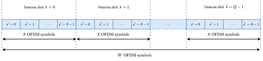
Figure 2: The BA phase spans a time window of $W$ OFDM symbols, which is divided into $Q$ beacons slots of $S$ OFDM symbols.

As depicted in Fig. 2 at the top of the next page, the BA phase is divided in $Q$ beacon slots of duration equal to $S$ consecutive OFDM blocks, i.e., $W=Q\,S$. At this point, let us denote with $\overline{y}^{(j,k_{i,\ell},s^{\prime})}(\widetilde{s})\triangleq\overline{y}^{(j,k_{i,\ell})}(\widetilde{s}\,S+s^{\prime})$ the polyphase decomposition of the received data (21) with respect to $S$, for $\widetilde{s}\in\{0,1,\ldots,Q-1\}$ and $s^{\prime}\in\{0,1,\ldots,S-1\}$. It assumed that the beamforming vectors $\widetilde{{\mathbf{u}}}^{(i,s)}_{\text{TX}}$ and ${\widetilde{{\mathbf{v}}}^{(j,s)}}$ are constant in each beacon slot, but they may vary from a beacon slot to another, i.e., $\widetilde{{\mathbf{u}}}^{(i,\widetilde{s}\,S+s^{\prime})}_{\text{TX}}\equiv\widetilde{{\mathbf{u}}}^{(i)}_{\text{TX}}(\widetilde{s})$ and $\widetilde{{\mathbf{v}}}^{(j,\widetilde{s}\,S+s^{\prime})}\equiv\widetilde{{\mathbf{v}}}^{(j)}(\widetilde{s})$. In this case, according to (21), one has

$$\overline{y}^{(j,k_{i,\ell},s^{\prime})}(\widetilde{s})=\sum_{\text{TX}\in\{\text{B},\text{J}\}}[\widetilde{{\mathbf{g}}}^{(j,i)}_{\text{TX}}(\widetilde{s})]^{\text{H}}\,{\text{vec}}\left(\widetilde{{\mathbf{C}}}_{\text{TX}}^{(k_{i,\ell})}\right)\\ \cdot d^{(k_{i,\ell},s^{\prime})}_{\text{TX}}(\widetilde{s})+\overline{w}^{(j,k_{i,\ell},s^{\prime})}(\widetilde{s})$$ (22)

where $\widetilde{{\mathbf{g}}}^{(j,i)}_{\text{TX}}(\widetilde{s})\triangleq[\widetilde{{\mathbf{u}}}^{(i)}_{\text{TX}}(\widetilde{s})]^{*}\otimes\widetilde{{\mathbf{v}}}^{(j)}(\widetilde{s})\in\mathbb{C}^{M_{\text{TX}}N_{\text{U}}}$, $d^{(k_{i,\ell},s^{\prime})}_{\text{TX}}(\widetilde{s})\triangleq d^{(k_{i,\ell})}_{\text{TX}}(\widetilde{s}\,S+s^{\prime})$, and noise sample $\overline{w}^{(j,k_{i,\ell},s^{\prime})}(\widetilde{s})\triangleq\overline{w}^{(j,k_{i,\ell})}(\widetilde{s}\,S+s^{\prime})$. We are considering the case of perfect beacon synchronization between BS and UE, as well as between the jammer and UE. Such an assumption is reasonable in practice since beacon slots are periodically repeated and, thus, terminals can easily acquire perfect knowledge of the start epoch of each beacon slot [11].

II-F Structure of the beamforming codebooks

To ensure spatial coverage, the size of the transmit and receive beamforming codebooks is proportional to the number of transmit and receive antennas. Therefore, for large-scale array in MMW communication, exhaustive search [40], although guaranteeing to select the optimal beam, introduces unacceptable beam training overhead. On the other hand, hierarchical schemes [41] require a non-trivial coordination among the UEs and the BS, which is difficult to have at the initial channel acquisition stage. Even though the proposed anti-jamming strategy can be applied to many available beamforming schemes, we resort herein to pseudo-random beamforming codebooks [11, 10, 42], which do not require interaction between the BS and each UE, and their overhead and complexity do not grow with the number of active users in the system. According to these schemes, the beamforming vectors of the transmitter TX and UE are

$$\widetilde{{\mathbf{u}}}^{(i)}_{\text{TX}}(\widetilde{s})=\frac{{\mathbf{1}}_{\mathcal{U}_{\text{TX}}^{(i)}(\widetilde{s})}}{\sqrt{U_{\text{TX}}}}\quad\text{and}\quad\widetilde{{\mathbf{v}}}^{(j)}(\widetilde{s})=\frac{{\mathbf{1}}_{\mathcal{V}^{(j)}(\widetilde{s})}}{\sqrt{V}}$$ (23)

respectively, where the angular support sets $\mathcal{U}_{\text{TX}}^{(i)}(\widetilde{s})\subseteq\{1,2,\ldots,M_{\text{TX}}\}$ and $\mathcal{V}^{(j)}(\widetilde{s})\subseteq\{1,2,\ldots,N_{\text{U}}\}$ of cardinality $U_{\text{TX}}\triangleq\left|\,\mathcal{U}_{\text{TX}}^{(i)}(\widetilde{s})\right|$ and $V\triangleq\left|\mathcal{V}^{(j)}(\widetilde{s})\right|$ collect the angles in the virtual beamspace channel representation that are probed by TX and sensed by the UE, respectively. So doing, the combined TX-UE beamforming vector in (22) reads as

$$\widetilde{{\mathbf{g}}}^{(j,i)}_{\text{TX}}(\widetilde{s})=\frac{{\mathbf{1}}_{\mathcal{U}_{\text{TX}}^{(i)}(\widetilde{s})}\otimes{\mathbf{1}}_{\mathcal{V}^{(j)}(\widetilde{s})}}{\sqrt{U_{\text{TX}}}\,\sqrt{V}}$$ (24)

whose entries are equal to $0$ or $1$ depending on the elements of the sets $\mathcal{U}_{\text{TX}}^{(i)}(\widetilde{s})$ and $\mathcal{V}^{(j)}(\widetilde{s})$.

The transmit beamforming codebook of the BS and the receive beamforming codebook of the UE are indeed pseudo-random since $\mathcal{U}_{\text{B}}^{(i)}(\widetilde{s})$, for $i\in\{1,2,\ldots,\widetilde{M}\}$, and $\mathcal{V}^{(j)}(\widetilde{s})$, for $j\in\{1,2,\ldots,\widetilde{N}_{\text{U}}\}$, are generated in a pseudo-random manner, for each beacon slot $\widetilde{s}\in\{0,1,\ldots,Q-1\}$. At each beacon slot, the subsets $\mathcal{U}_{\text{B}}^{(i)}(\widetilde{s})$, for $i\in\{1,2,\ldots,\widetilde{M}\}$, are perfectly known at the UE, whereas $\mathcal{V}^{(j)}(\widetilde{s})$, for $j\in\{1,2,\ldots,\widetilde{N}_{\text{U}}\}$, are locally and independently generated by the UE. As regards the jammer, the transmit beamforming codebook $\mathcal{U}_{\text{J}}^{(i)}(\widetilde{s})$ is assumed to be unknown at the UE, for each beacon slot and $i\in\{1,2,\ldots,\widetilde{M}\}$. The impact of the choice of the jamming codebook on the BA procedure between the BS and the UE is discussed in Section III.

II-G Probing symbols of the BS in conventional schemes

Conventional BA schemes [6, 7, 8, 9, 10, 11, 12, 13, 14, 15, 16, 17, 18, 19, 20, 21, 22, 23, 24, 25] do not account for jamming attacks. In such jammer-unaware methods, the BS transmits known probing symbols during each beacon slot:

$$d^{(k_{i,\ell})}_{\text{B}}(s)=\sqrt{\mathcal{P}_{\text{B}}}\,t^{(k_{i,\ell})}(s)$$ (25)

where $t^{(k_{i,\ell})}(s)\in\mathbb{C}$ is a publicly known symbol corresponding to the $i$-th stream in the $s$-th block on subcarrier $k_{i,\ell}$, with $|t^{(k_{i,\ell})}(s)|^{2}=1$, for $\ell\in\{0,1,\ldots,F_{i}-1\}$, and $\mathcal{P}_{\text{B}}$ is the available power per symbol at the BS. In Section IV, we will suitably modify the transmission scheme (25) to confer anti-jamming capabilities to the BA procedure.

II-H Probing symbols of the jammer

The probing symbols transmitted by the jammer are essentially a noisy version of the publicly known probing symbols $\{t^{(k_{i,\ell})}(s)\}$ and they are modeled as

$$d^{(k_{i,\ell})}_{\text{J}}(s)=\sqrt{(1-\gamma_{\text{J}})\,\mathcal{P}_{\text{J}}}\,t^{(k_{i,\ell})}(s)+\sqrt{\gamma_{\text{J}}\,\mathcal{P}_{\text{J}}}\,r^{(k_{i,\ell})}_{\text{J}}(s)$$ (26)

where $\mathcal{P}_{\text{J}}$ is the available power per symbol of the jammer and each stream $\{r^{(k_{i,\ell})}_{\text{J}}(s)\}$ is modeled as a sequence of zero-mean unit-variance independent and identically distributed (i.i.d.) complex circular RVs. For the sake of generality, we have introduced in (26) a power factor $0\leq\gamma_{\text{J}}\leq 1$ that allows us to account for different jamming attacks. In extreme cases, the jammer may exclusively transmit known probing symbols, i.e., $\gamma_{\text{J}}=0$ or, on the other hand, it might send in the air noise only, i.e., $\gamma_{\text{J}}=1$. In the intermediate case $0<\gamma_{\text{J}}<1$, the jammer could decide to split its available power between known probing symbols and intentional noise.

III Jammer-unaware beam alignment

In this section, we show what is the impact of transmit beamforming codebook of the jammer on the BA acquisition performance when the BS uses the conventional probing scheme (25) in the presence of the jamming attack. In this situation, the received signal by the UE is obtained by substituting (25) and (26) into (22), thus obtaining

$$\overline{y}^{(j,k_{i,\ell},s^{\prime})}(\widetilde{s})=\sqrt{\mathcal{P}_{\text{B}}}\,\widetilde{h}^{(j,i,k_{i,\ell})}_{\text{B}}(\widetilde{s})\,t^{(k_{i,\ell},s^{\prime})}(\widetilde{s})\\ +\widetilde{h}^{(j,i,k_{i,\ell})}_{\text{J}}(\widetilde{s})\left[\sqrt{(1-\gamma_{\text{J}})\,\mathcal{P}_{\text{J}}}\,t^{(k_{i,\ell})}(s)\right.\\ \left.+\sqrt{\gamma_{\text{J}}\,\mathcal{P}_{\text{J}}}\,r^{(k_{i,\ell},s^{\prime})}_{\text{J}}(\widetilde{s})\right]+\overline{w}^{(j,k_{i,\ell},s^{\prime})}(\widetilde{s})$$ (27)

where $\widetilde{s}\in\{0,1,\ldots,Q-1\}$ and $s^{\prime}\in\{0,1,\ldots,S-1\}$, with $\widetilde{h}^{(j,i,k_{i,\ell})}_{\text{TX}}(\widetilde{s})\triangleq[\widetilde{{\mathbf{g}}}^{(j,i)}_{\text{TX}}(\widetilde{s})]^{\text{H}}\,{\text{vec}}\left(\widetilde{{\mathbf{C}}}_{\text{TX}}^{(k_{i,\ell})}\right)$, $t^{(k_{i,\ell},s^{\prime})}(\widetilde{s})\triangleq t^{(k_{i,\ell})}(\widetilde{s}\,S+s^{\prime})$, and $r^{(k_{i,\ell},s^{\prime})}_{\text{J}}(\widetilde{s})\triangleq r^{(k_{i,\ell})}_{\text{J}}(\widetilde{s}\,S+s^{\prime})$. With reference to the beacon slot $\widetilde{s}\in\{0,1,\ldots,Q-1\}$ (see Fig. 2), by stacking $S$ consecutive samples (27) into the vector

$$\overline{{\mathbf{y}}}^{(j,k_{i,\ell})}(\widetilde{s})\triangleq[\overline{y}^{(j,k_{i,\ell},0)}(\widetilde{s}),\overline{y}^{(j,k_{i,\ell},1)}(\widetilde{s}),\\ \ldots,\overline{y}^{(j,k_{i,\ell},S-1)}(\widetilde{s})]^{\text{T}}\in\mathbb{C}^{S}$$ (28)

one obtains

$$\overline{{\mathbf{y}}}^{(j,k_{i,\ell})}(\widetilde{s})=\sqrt{\mathcal{P}_{\text{B}}}\,\widetilde{h}^{(j,i,k_{i,\ell})}_{\text{B}}(\widetilde{s})\,{\mathbf{t}}^{(k_{i,\ell})}(\widetilde{s})\\ +\widetilde{h}^{(j,i,k_{i,\ell})}_{\text{J}}(\widetilde{s})\left[\sqrt{(1-\gamma_{\text{J}})\,\mathcal{P}_{\text{J}}}\,{\mathbf{t}}^{(k_{i,\ell})}(\widetilde{s})\right.\\ \left.+\sqrt{\gamma_{\text{J}}\,\mathcal{P}_{\text{J}}}\,{\mathbf{r}}_{\text{J}}^{(k_{i,\ell})}(\widetilde{s})\right]+\overline{{\mathbf{w}}}^{(j,k_{i,\ell})}(\widetilde{s})$$ (29)

where

$${\mathbf{t}}^{(k_{i,\ell})}(\widetilde{s}) \triangleq[t^{(k_{i,\ell},0)}(\widetilde{s}),t^{(k_{i,\ell},1)}(\widetilde{s}),$$

$$\hskip 56.9055pt\ldots,t^{(k_{i,\ell},S-1)}(\widetilde{s})]^{\text{T}}\in\mathbb{C}^{S}$$

$${\mathbf{r}}_{\text{J}}^{(k_{i,\ell})}(\widetilde{s}) \triangleq[r_{\text{J}}^{(k_{i,\ell},0)}(\widetilde{s}),r_{\text{J}}^{(k_{i,\ell},1)}(\widetilde{s}),$$

$$\hskip 56.9055pt\ldots,r_{\text{J}}^{(k_{i,\ell},S-1)}(\widetilde{s})]^{\text{T}}\in\mathbb{C}^{S}$$

$$\overline{{\mathbf{w}}}^{(j,k_{i,\ell})}(\widetilde{s}) \triangleq[\overline{w}^{(j,k_{i,\ell},0)}(\widetilde{s}),\overline{w}^{(j,k_{i,\ell},1)}(\widetilde{s}),$$

$$\hskip 56.9055pt\ldots,\overline{w}^{(j,k_{i,\ell},S-1)}(\widetilde{s})]^{\text{T}}\in\mathbb{C}^{S}\>.$$

The strongest multipath components of the legitimate channel correspond to the entries with large variance of the channel matrix $\overline{{\mathbf{C}}}_{\text{B}}^{(k)}$, which is defined in (17) and represented by (18), for $k\in\{0,1,\ldots,F-1\}$. To identify the variance of such components and, thus, achieve successfully BA, several objective functions can be used in a jammer-unaware approach [7, 8, 9, 10, 11, 12, 13, 14, 15, 16, 17, 18, 19, 20, 21, 22, 23, 24, 25]. Herein, we focus on the second-order objective function introduced in [11] that can be expressed as

$$P^{(j,i)}(\widetilde{s})=\frac{1}{S\,F_{i}}\sum_{\ell=0}^{F_{i}-1}{\mathbb{E}}\left[\left\|\overline{{\mathbf{y}}}^{(j,k_{i,\ell})}(\widetilde{s})\right\|_{2}^{2}\right]$$ (30)

which represents the (normalized) mean received power of the $i$-th data stream at the output of the $j$-th RF chain during the $\widetilde{s}$-th beacon slot, where the expectation is also evaluated with respect to the random probing symbols transmitted by the jammer. By substituting (29) into (30) and invoking the statistically independence among channels, random sequences, and noise, one has

$$P^{(j,i)}(\widetilde{s})=[{{\mathbf{g}}}^{(j,i)}_{\text{B}}(\widetilde{s})]^{\text{T}}\,\boldsymbol{\xi}_{\text{B}}+[{{\mathbf{g}}}^{(j,i)}_{\text{J}}(\widetilde{s})]^{\text{T}}\,\boldsymbol{\xi}_{\text{J}}+\sigma^{2}_{w}$$ (31)

where we have additionally observed that

$${\mathbb{E}}\left[|\widetilde{h}^{(j,i,k_{i,\ell})}_{\text{TX}}(\widetilde{s})|^{2}\right] =[\widetilde{{\mathbf{g}}}^{(j,i)}_{\text{TX}}(\widetilde{s})]^{\text{H}}\,{\mathbf{R}}_{\widetilde{{\mathbf{C}}}_{\text{TX}}}\,\widetilde{{\mathbf{g}}}^{(j,i)}_{\text{TX}}(\widetilde{s})$$

$$=[{{\mathbf{g}}}^{(j,i)}_{\text{TX}}(\widetilde{s})]^{\text{T}}\,\boldsymbol{\xi}_{\text{TX}}$$ (32)

with

$${\mathbf{R}}_{\widetilde{{\mathbf{C}}}_{\text{TX}}}\triangleq{\mathbb{E}}\left[{\text{vec}}\left(\widetilde{{\mathbf{C}}}_{\text{TX}}^{(k_{i,\ell})}\right)\,{\text{vec}}^{\text{H}}\left(\widetilde{{\mathbf{C}}}_{\text{TX}}^{(k_{i,\ell})}\right)\right]\\ \in\mathbb{C}^{(M_{\text{TX}}N_{\text{U}})\times(M_{\text{TX}}N_{\text{U}})}$$ (33)

being the covariance matrix of the vectorized beamspace representation of the channel matrix. It is worth noting that, under the assumption that the virtual channel coefficients are uncorrelated., the matrix ${\mathbf{R}}_{\widetilde{{\mathbf{C}}}_{\text{TX}}}$ is diagonal with some dominant components along the diagonal and, according to (19), it turns out to be independent of the subcarrier index $k_{i,\ell}$. In (32), we set ${{\mathbf{g}}}^{(j,i)}_{\text{TX}}(\widetilde{s})\triangleq\sqrt{U_{\text{TX}}}\,\sqrt{V}\,\widetilde{{\mathbf{g}}}^{(j,i)}_{\text{TX}}(\widetilde{s})$, with the combined TX-UE beamforming vector $\widetilde{{\mathbf{g}}}^{(j,i)}_{\text{TX}}(\widetilde{s})$ given by (24), whereas

$$\boldsymbol{\xi}_{\text{TX}}\triangleq\frac{\mathcal{P}_{\text{TX}}}{U_{\text{TX}}\,V}\left[\{{\mathbf{R}}_{\widetilde{{\mathbf{C}}}_{\text{TX}}}\}_{1,1},\{{\mathbf{R}}_{\widetilde{{\mathbf{C}}}_{\text{TX}}}\}_{2,2},\right.\\ \left.\ldots,\{{\mathbf{R}}_{\widetilde{{\mathbf{C}}}_{\text{TX}}}\}_{M_{\text{TX}}N_{\text{U}},M_{\text{TX}}N_{\text{U}}}\right]^{\text{T}}\in\mathbb{R}^{M_{\text{TX}}N_{\text{U}}}\>.$$ (34)

Within this section, we assume that $\sigma_{w}^{2}$ is known at the UE for beam determination. We remember that the vector ${{\mathbf{g}}}^{(j,i)}_{\text{B}}(\widetilde{s})$ is known at the UE, for all values of $j\in\{1,2,\ldots,\widetilde{N}_{\text{U}}\}$, $i\in\{1,2,\ldots,\widetilde{M}\}$, and $\widetilde{s}\in\{0,1,\ldots,Q-1\}$. On the other hand, ${{\mathbf{g}}}^{(j,i)}_{\text{J}}(\widetilde{s})$ is unknown at the UE, since it does not have knowledge of both the transmit number of antennas $M_{\text{J}}$ and beamforming codebook $\mathcal{U}_{\text{J}}^{(i)}(\widetilde{s})$ of the jammer. The unknown vector $\boldsymbol{\xi}_{\text{B}}$ has to be estimated to identify the AoA-AoD directions of the strongest scatterers regarding the BS-to-UE channel. To this aim, the UE can collect all the available power measurements in the vector

$${\mathbf{p}}\triangleq[P^{(1,1)}(0),\ldots,P^{(\widetilde{N}_{\text{U}},\widetilde{M})}(0),\\ P^{(1,1)}(1),\ldots,P^{(\widetilde{N}_{\text{U}},\widetilde{M})}(1),\ldots,\\ P^{(1,1)}(Q-1),\ldots,P^{(\widetilde{N}_{\text{U}},\widetilde{M})}(Q-1)]^{\text{T}}\\ ={\mathbf{G}}_{\text{B}}\,\boldsymbol{\xi}_{\text{B}}+{\mathbf{G}}_{\text{J}}\,\boldsymbol{\xi}_{\text{J}}+\sigma^{2}_{w}\,{\mathbf{1}}_{\widetilde{M}\widetilde{N}_{\text{U}}Q}$$ (35)

with

$${\mathbf{G}}_{\text{TX}}\triangleq[{{\mathbf{g}}}^{(1,1)}_{\text{TX}}(0),\ldots,{{\mathbf{g}}}^{(\widetilde{N}_{\text{U}},\widetilde{M})}_{\text{TX}}(0),\\ {{\mathbf{g}}}^{(1,1)}_{\text{TX}}(1),\ldots,{{\mathbf{g}}}^{(\widetilde{N}_{\text{U}},\widetilde{M})}_{\text{TX}}(1),\ldots,\\ {{\mathbf{g}}}^{(1,1)}_{\text{TX}}(Q-1),\ldots,{{\mathbf{g}}}^{(\widetilde{N}_{\text{U}},\widetilde{M})}_{\text{TX}}(Q-1)]^{\text{T}}\\ \in\mathbb{R}^{(\widetilde{M}\widetilde{N}_{\text{U}}Q)\times(M_{\text{TX}}N_{\text{U}})}\>.$$ (36)

The model (35) represents a high-dimensional system in which the number of unknowns $M_{\text{B}}\,N_{\text{U}}$ is at least of the same order of magnitude as the number of observations $\widetilde{M}\,\widetilde{N}_{\text{U}}\,Q$ or, even, $M_{\text{B}}\,N_{\text{U}}\gg\widetilde{M}\,\widetilde{N}_{\text{U}}\,Q$, in which case one cannot hope to recover the desired vector $\boldsymbol{\xi}_{\text{B}}$ if it does not exhibit any particular structure. However, the vector $\boldsymbol{\xi}_{\text{B}}$ is sparse and its entries are non-negative, i.e., $\boldsymbol{\xi}_{\text{B}}\geq{\mathbf{0}}_{M_{\text{B}}N_{\text{U}}}$. If the UE is unaware of the jamming attack, an estimate of $\boldsymbol{\xi}_{\text{B}}$ can be obtained by solving the non-negative least-squares (NNLS) problem:

$$\widehat{\boldsymbol{\xi}}_{\text{B}}=\arg\min_{\boldsymbol{\xi}_{\text{B}}^{\star}\in\mathbb{R}^{M_{\text{B}}N_{\text{U}}}}\left\|{\mathbf{p}}-{\mathbf{G}}_{\text{B}}\,\boldsymbol{\xi}_{\text{B}}^{\star}-\sigma^{2}_{w}\,{\mathbf{1}}_{\widetilde{M}\widetilde{N}_{\text{U}}Q}\right\|_{2}^{2}\>,\\ \quad\text{subject to $\boldsymbol{\xi}_{\text{B}}^{\star}\geq{\mathbf{0}}_{M_{\text{B}}N_{\text{U}}}$}$$ (37)

which is a convex optimization problem that can be solved efficiently [43]. In the absence of the jamming attack, under mild conditions on the matrix ${\mathbf{G}}_{\text{B}}$, the non-negativity constraint $\boldsymbol{\xi}_{\text{B}}^{\star}\geq{\mathbf{0}}_{M_{\text{B}}N_{\text{U}}}$ alone suffices for sparse recovery of $\boldsymbol{\xi}_{\text{B}}$, without the need to employ sparsity-promoting regularization terms [44]. The minimization program (37) is directly implemented in MATLAB as the function lsqnonneg, which executes the active-set algorithm of Lawson and Hanson [45].

In practice, the NNLS problem to be solved comes from replacing ${\mathbf{p}}$ in (37) with the corresponding estimate

$$\widehat{{\mathbf{p}}}\triangleq[\widehat{P}^{(1,1)}(0),\ldots,\widehat{P}^{(\widetilde{N}_{\text{U}},\widetilde{M})}(0),\\ \widehat{P}^{(1,1)}(1),\ldots,\widehat{P}^{(\widetilde{N}_{\text{U}},\widetilde{M})}(1),\ldots,\\ \widehat{P}^{(1,1)}(Q-1),\ldots,\widehat{P}^{(\widetilde{N}_{\text{U}},\widetilde{M})}(Q-1)]^{\text{T}}$$ (38)

where

$$\widehat{P}^{(j,i)}(\widetilde{s})=\frac{1}{S\,F_{i}}\sum_{\ell=0}^{F_{i}-1}\left\|\overline{{\mathbf{y}}}^{(j,k_{i,\ell})}(\widetilde{s})\right\|_{2}^{2}$$ (39)

for $j\in\{1,2,\ldots,\widetilde{N}_{\text{U}}\}$ and $i\in\{1,2,\ldots,\widetilde{M}\}$, within beacon slot $\widetilde{s}\in\{0,1,\ldots,Q-1\}$.

III-A Error analysis

As it is apparent from (35), the impact of the jamming attack on the BA procedure between the BS and the UE is determined by the transmit beamforming codebook of the jammer, which appears in the matrix ${\mathbf{G}}_{\text{J}}$, and the second-order statistics of the channel between the jammer and the UE, i.e., the sparse vector $\boldsymbol{\xi}_{\text{J}}$. The solution of (37) approximates $\boldsymbol{\xi}_{\text{B}}$ with an error

$$\mathcal{E}(\widehat{\boldsymbol{\xi}}_{\text{B}})\triangleq\|\boldsymbol{\xi}_{\text{B}}-\widehat{\boldsymbol{\xi}}_{\text{B}}\|_{2}$$ (40)

which depends not only on the jamming contribution ${\mathbf{G}}_{\text{J}}\,\boldsymbol{\xi}_{\text{J}}$, but also on the fact that $\boldsymbol{\xi}_{\text{B}}$ is not exactly sparse, i.e., only a small number of its entries are nonzero, but $\boldsymbol{\xi}_{\text{B}}$ is only close to a sparse vector. More precisely, a vector ${\mathbf{s}}_{\text{TX}}\in\mathbb{R}^{M_{\text{TX}}N_{\text{U}}}$is called $\kappa_{\text{TX}}$-sparse [46, Def. 2.1] if at most $\kappa_{\text{TX}}$ of its entries are nonzero, i.e., $|\text{supp}({\mathbf{s}}_{\text{TX}})|\leq\kappa_{\text{TX}}$, for $\text{TX}\in\{\text{B},\text{J}\}$. The best $\kappa_{\text{TX}}$-term approximation of $\boldsymbol{\xi}_{\text{TX}}$ is defined as (see, e.g., [46, Def. 2.2])

$$\sigma_{\kappa_{\text{TX}}}(\boldsymbol{\xi}_{\text{TX}})\triangleq\inf\Big{\{}\|\boldsymbol{\xi}_{\text{TX}}-{\mathbf{s}}_{\text{TX}}\|_{1},\text{where ${\mathbf{s}}_{\text{TX}}\in\mathbb{R}^{M_{\text{TX}}N_{\text{U}}}$}\\ \text{is $\kappa_{\text{TX}}$-sparse}\Big{\}}\>.$$ (41)

The infimum is achieved in (41) by a $\kappa_{\text{TX}}$-sparse vector ${\mathbf{s}}_{\text{TX}}\in\mathbb{C}^{M_{\text{TX}}N_{\text{U}}}$ whose nonzero entries equal the $\kappa_{\text{TX}}$ largest absolute entries of $\boldsymbol{\xi}_{\text{TX}}$. As regards to the transmit beamforming codebook of the jammer, we study the two different cases ${\mathbf{G}}_{\text{J}}\neq{\mathbf{G}}_{\text{B}}$ and ${\mathbf{G}}_{\text{J}}={\mathbf{G}}_{\text{B}}$ separately.

III-A1 ${\mathbf{G}}_{\text{J}}\neq{\mathbf{G}}_{\text{B}}$

In principle, the transmit beamforming codebooks of the BS and jammer may be different. For instance, the jamming codebook $\widetilde{{\mathbf{u}}}^{(i)}_{\text{J}}(\widetilde{s})$ might be chosen in a pseudo-random manner similarly to the BS or, if the jammer is a high-power device that has a large amount of power to be spent, another option for the jammer could consist of probing the channel along all the possible directions (referred to as omnidirectional beamforming) and, consequently, setting $\widetilde{{\mathbf{u}}}^{(i)}_{\text{J}}(\widetilde{s})={\mathbf{1}}_{\widetilde{M}}/\sqrt{\widetilde{M}}$. In the case of ${\mathbf{G}}_{\text{J}}\neq{\mathbf{G}}_{\text{B}}$, the jamming contribution ${\mathbf{G}}_{\text{J}}\,\boldsymbol{\xi}_{\text{J}}$ appears as additional noise of arbitrary nature and the reconstruction error (40) can be upper bounded [47] as follows

$$\mathcal{E}(\widehat{\boldsymbol{\xi}}_{\text{B}})\leq\frac{A_{1}}{\sqrt{\kappa_{\text{B}}}}\,\sigma_{\kappa_{\text{B}}}(\boldsymbol{\xi}_{\text{B}})+A_{2}\,\|{\mathbf{G}}_{\text{J}}\,\boldsymbol{\xi}_{\text{J}}\|_{2}$$ (42)

for some constants $A_{1},A_{2}>0$, provided that the matrix ${\mathbf{G}}_{\text{B}}$ satisfies the conditions summarized in the Appendix. By resorting to the sub-multiplicative property of the $\ell_{2}$ norm [35], one has

$$\|{\mathbf{G}}_{\text{J}}\,\boldsymbol{\xi}_{\text{J}}\|_{2} \leq\sqrt{{\text{trace}}({\mathbf{G}}_{\text{J}}\,{\mathbf{G}}_{\text{J}}^{\text{T}})}\,\|\boldsymbol{\xi}_{\text{J}}\|_{2}$$

$$=\frac{\mathcal{P}_{\text{J}}}{U_{\text{J}}\,V}\sqrt{\sum_{\shortstack{\footnotesize$i\in\{1,2,\ldots,\widetilde{M}\}$ \\ \footnotesize$j\in\{1,2,\ldots,\widetilde{N}_{\text{U}}\}$ \\ \footnotesize$\widetilde{s}\in\{0,1,\ldots,Q-1\}$}}\left\|{\mathbf{1}}_{\mathcal{U}_{\text{J}}^{(i)}(\widetilde{s})}\otimes{\mathbf{1}}_{\mathcal{V}^{(j)}(\widetilde{s})}\right\|_{2}^{2}}$$

$$\hskip 71.13188pt\cdot\sqrt{\sum_{n=1}^{M_{\text{J}}N_{\text{U}}}\{{\mathbf{R}}_{\widetilde{{\mathbf{C}}}_{\text{J}}}\}_{n,n}^{2}}$$

$$\leq\frac{\mathcal{P}_{\text{J}}}{U_{\text{J}}\,V}\,\sqrt{\widetilde{M}\,\widetilde{N}_{\text{U}}\,Q\,M_{\text{J}}\,N_{\text{U}}}\,\sqrt{\sum_{n=1}^{M_{\text{J}}N_{\text{U}}}\{{\mathbf{R}}_{\widetilde{{\mathbf{C}}}_{\text{J}}}\}_{n,n}^{2}}$$ (43)

where we have also used (24) and (36), and remembered that ${{\mathbf{g}}}^{(j,i)}_{\text{J}}(\widetilde{s})=\sqrt{U_{\text{J}}}\,\sqrt{V}\,\widetilde{{\mathbf{g}}}^{(j,i)}_{\text{J}}(\widetilde{s})$. It is apparent from (43) that probing more directions simultaneously (i.e., increasing $U_{\text{J}}$) has the detrimental effect from the jammer’s viewpoint of spreading the total power over all such directions, thereby obtaining a worse power concentration in the angle domain.

III-A2 ${\mathbf{G}}_{\text{J}}={\mathbf{G}}_{\text{B}}$

The jammer might transmit by using the same beamforming codebook of the BS that we remember to be known to all UEs a priori, i.e., $\mathcal{U}_{\text{J}}^{(i)}(\widetilde{s})\equiv\mathcal{U}_{\text{B}}^{(i)}(\widetilde{s})$, for any $i\in\{1,2,\ldots,\widetilde{M}\}$ and $\widetilde{s}\in\{0,1,\ldots,Q-1\}$, which necessarily requires that $M_{\text{J}}=M_{\text{B}}\equiv M$. In this case, one has ${\mathbf{G}}_{\text{J}}={\mathbf{G}}_{\text{B}}\equiv{\mathbf{G}}$ and, consequently, eq. (35) ends up to

$${\mathbf{p}}={\mathbf{G}}\,(\boldsymbol{\xi}_{\text{B}}+\boldsymbol{\xi}_{\text{J}})+\sigma^{2}_{w}\,{\mathbf{1}}_{\widetilde{M}\widetilde{N}_{\text{U}}Q}$$ (44)

which shows that the UE sees the sum of two sparse vectors $\boldsymbol{\xi}_{\text{B}}$ and $\boldsymbol{\xi}_{\text{J}}$ under the same measurement matrix ${\mathbf{G}}$. This case is worse than the previous one when ${\mathbf{G}}_{\text{J}}\neq{\mathbf{G}}_{\text{B}}$ since $\widehat{\boldsymbol{\xi}}_{\text{B}}$ turns out to be an estimate of $\boldsymbol{\xi}_{\text{B}}+\boldsymbol{\xi}_{\text{J}}$. In this worst case, successful BA between the BS and the UE is achieved if

$$\frac{\mathcal{P}_{\text{B}}}{\mathcal{P}_{\text{J}}}\gg\frac{\max_{n\in\{1,2,\ldots,MN_{\text{U}}\}}\{{\mathbf{R}}_{\widetilde{{\mathbf{C}}}_{\text{J}}}\}_{n,n}}{\max_{n\in\{1,2,\ldots,MN_{\text{U}}\}}\{{\mathbf{R}}_{\widetilde{{\mathbf{C}}}_{\text{B}}}\}_{n,n}}\>.$$ (45)

Condition (45) is violated when the jammer transmits with a power $\mathcal{P}_{\text{J}}$ sufficiently greater than $\mathcal{P}_{\text{B}}$ and/or, compared to the BS, it has a more favorable propagation towards the UE.

IV The proposed anti-jamming beam alignment scheme

In this section, we modify the transmit scheme of the BS in order to allow the UE to cancel the jamming contribution. A key ingredient of our proposed anti-jamming scheme is the random probing symbols transmitted by the BS, which follow the model

$$d^{(k_{i,\ell})}_{\text{B}}(s)=\sqrt{[1-\gamma_{\text{B}}(s)]\,\mathcal{P}_{\text{B}}}\,t^{(k_{i,\ell})}(s)+\sqrt{\gamma_{\text{B}}(s)\,\mathcal{P}_{\text{B}}}\,r^{(k_{i,\ell})}_{\text{B}}(s)$$ (46)

where each stream $\{r^{(k_{i,\ell})}_{\text{B}}(s)\}$ is modeled as a sequence of zero-mean unit-variance i.i.d. complex circular RVs, with $r^{(k_{i,\ell})}_{\text{B}}(s)$ and (26) mutually independent and statistically independent of noise $\overline{w}^{(j,k_{i,\ell})}(s)$, for each OFDM block, and for any $i\in\{1,2,\ldots,\widetilde{M}\}$ and $\forall j\in\{1,2,\ldots,\widetilde{N}_{\text{U}}\}$. The BS allocates a different fraction $0\leq\gamma_{\text{B}}(s)\leq 1$ of $\mathcal{P}_{\text{B}}$ to the random symbols $r^{(k_{i,\ell})}_{\text{B}}(s)$. Since $\{r^{(k_{i,\ell})}_{\text{B}}(s)\}$ is randomly generated at the BS, it is unknown at the UE. However, the UE knows that the BS has superimposed the random sequence $\{r^{(k_{i,\ell})}_{\text{B}}(s)\}$ on the known sequence $\{t^{(k_{i,\ell})}(s)\}$ and it can use such a knowledge to undo the jamming attack. The conventional probing scheme (25) can be obtained from (46) by setting $\gamma_{\text{B}}(s)=0$, $\forall s\in\{0,1,\ldots,W-1\}$.

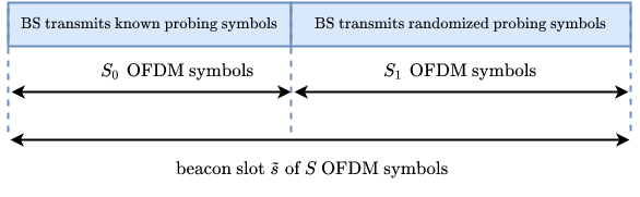
Figure 3: Each beacon slot is divided into two subslots: during the first $S_{0}$ OFDM symbols, the BS transmits a known probing sequence, whereas a random sequence is superimposed to the known symbols in the remaining $S_{1}$ OFDM blocks, with $S_{0}+S_{1}=S$.

In the sequel, we assume that $\gamma_{\text{B}}(s)$ does not vary from a beacon slot to another, but it might assume different values within a beacon slot, i.e, $\gamma_{\text{B}}(\widetilde{s}\,S+s^{\prime})\equiv\gamma_{\text{B}}^{(s^{\prime})}$, for any $\widetilde{s}\in\{0,1,\ldots,Q-1\}$ and $s^{\prime}\in\{0,1,\ldots,S-1\}$. To counteract the detrimental effect of the jamming attack, we additionally propose to divide each beacon slot $\widetilde{s}$ in two subslots (see Fig. 3): in the former one, which lasts $S_{0}$ OFDM symbols, the BS transmits only the known symbols $t^{(k_{i,\ell},s^{\prime})}$ defined in Section III, i.e., $\gamma_{\text{B}}^{(s^{\prime})}=0$, for $s^{\prime}\in\{0,1,\ldots,S_{0}-1\}$; whereas in the remaining $S_{1}\triangleq S-S_{0}$ OFDM symbols of each beacon slot, the BS superimposes the random sequence $r^{(k_{i,\ell},s^{\prime})}_{\text{B}}(\widetilde{s})\triangleq r^{(k_{i,\ell})}_{\text{B}}(\widetilde{s}\,S+s^{\prime})$ to the known symbols $t^{(k_{i,\ell},s^{\prime})}$, with a fixed power fraction $\gamma_{\text{B}}^{(s^{\prime})}\equiv\gamma_{\text{B}}\in(0,1]$, for all $s^{\prime}\in\{S_{0},S_{0}+1,\ldots,S-1\}$.

By substituting (26) and (46) into (22), one has

$$\overline{y}^{(j,k_{i,\ell},s^{\prime})}(\widetilde{s})=\widetilde{h}^{(j,i,k_{i,\ell})}_{\text{B}}(\widetilde{s})\left\{\sqrt{[1-\gamma_{\text{B}}^{(s^{\prime})}]\,\mathcal{P}_{\text{B}}}\,t^{(k_{i,\ell},s^{\prime})}(\widetilde{s})\right.\\ \left.+\sqrt{\gamma_{\text{B}}^{(s^{\prime})}\,\mathcal{P}_{\text{B}}}\,r_{\text{B}}^{(k_{i,\ell},s^{\prime})}(\widetilde{s})\right\}\\ +\widetilde{h}^{(j,i,k_{i,\ell})}_{\text{J}}(\widetilde{s})\left\{\sqrt{(1-\gamma_{\text{J}})\,\mathcal{P}_{\text{J}}}\,t^{(k_{i,\ell},s^{\prime})}(\widetilde{s})\right.\\ \left.+\sqrt{\gamma_{\text{J}}\,\mathcal{P}_{\text{J}}}\,r^{(k_{i,\ell},s^{\prime})}_{\text{J}}(\widetilde{s})\right\}+\overline{w}^{(j,k_{i,\ell},s^{\prime})}(\widetilde{s})$$ (47)

where $\widetilde{s}\in\{0,1,\ldots,Q-1\}$ and $s^{\prime}\in\{0,1,\ldots,S-1\}$, with $\widetilde{h}^{(j,i,k_{i,\ell})}_{\text{TX}}(\widetilde{s})$, and $r^{(k_{i,\ell},s^{\prime})}_{\text{J}}(\widetilde{s})$ defined in Section III. According to the proposed protocol, the data block (29) received by the UE during the beacon slot $\widetilde{s}\in\{0,1,\ldots,Q-1\}$ can be partitioned as

$$\overline{{\mathbf{y}}}^{(j,k_{i,\ell})}(\widetilde{s})=\begin{bmatrix}\overline{{\mathbf{y}}}_{0}^{(j,k_{i,\ell})}(\widetilde{s})\\ \overline{{\mathbf{y}}}_{1}^{(j,k_{i,\ell})}(\widetilde{s})]\end{bmatrix}\>,\\ \text{with $\overline{{\mathbf{y}}}_{0}^{(j,k_{i,\ell})}(\widetilde{s})\in\mathbb{C}^{S_{0}}$ and $\overline{{\mathbf{y}}}_{1}^{(j,k_{i,\ell})}(\widetilde{s})\in\mathbb{C}^{S_{1}}$}$$ (48)

for $j\in\{1,2,\ldots,\widetilde{N}_{\text{U}}\}$, $i\in\{1,2,\ldots,\widetilde{M}\}$, and beacon slot $\widetilde{s}\in\{0,1,\ldots,Q-1\}$, with

$$\overline{{\mathbf{y}}}_{0}^{(j,k_{i,\ell})}(\widetilde{s})=\sqrt{\mathcal{P}_{\text{B}}}\,\widetilde{h}^{(j,i,k_{i,\ell})}_{\text{B}}(\widetilde{s})\,{\mathbf{t}}_{0}^{(k_{i,\ell})}(\widetilde{s})\\ +\widetilde{h}^{(j,i,k_{i,\ell})}_{\text{J}}(\widetilde{s})\left\{\sqrt{(1-\gamma_{\text{J}})\,\mathcal{P}_{\text{J}}}\,{\mathbf{t}}_{0}^{(k_{i,\ell})}(\widetilde{s})\right.\\ \left.+\sqrt{\gamma_{\text{J}}\,\mathcal{P}_{\text{J}}}\,{\mathbf{r}}_{0,\text{J}}^{(k_{i,\ell})}(\widetilde{s})\right\}+\overline{{\mathbf{w}}}_{0}^{(j,k_{i,\ell})}(\widetilde{s})$$ (49)

$$\overline{{\mathbf{y}}}_{1}^{(j,k_{i,\ell})}(\widetilde{s})=\widetilde{h}^{(j,i,k_{i,\ell})}_{\text{B}}(\widetilde{s})\left\{\sqrt{(1-\gamma_{\text{B}})\,\mathcal{P}_{\text{B}}}\,{\mathbf{t}}_{1}^{(k_{i,\ell})}(\widetilde{s})\right.\\ \left.+\sqrt{\gamma_{\text{B}}\,\mathcal{P}_{\text{B}}}\,{\mathbf{r}}_{1,\text{B}}^{(k_{i,\ell})}(\widetilde{s})\right\}+\widetilde{h}^{(j,i,k_{i,\ell})}_{\text{J}}(\widetilde{s})\left\{\sqrt{(1-\gamma_{\text{J}})\,\mathcal{P}_{\text{J}}}\,{\mathbf{t}}_{1}^{(k_{i,\ell})}(\widetilde{s})\right.\\ \left.+\sqrt{\gamma_{\text{J}}\,\mathcal{P}_{\text{J}}}\,{\mathbf{r}}_{1,\text{J}}^{(k_{i,\ell})}(\widetilde{s})\right\}+\overline{{\mathbf{w}}}_{1}^{(j,k_{i,\ell})}(\widetilde{s})$$ (50)

where ${\mathbf{t}}_{0}^{(k_{i,\ell})}(\widetilde{s})\in\mathbb{C}^{S_{0}}$, ${\mathbf{t}}_{1}^{(k_{i,\ell})}(\widetilde{s})\in\mathbb{C}^{S_{1}}$, ${\mathbf{r}}_{0,\text{J}}^{(k_{i,\ell})}(\widetilde{s})\in\mathbb{C}^{S_{0}}$, ${\mathbf{r}}_{1,\text{J}}^{(k_{i,\ell})}(\widetilde{s})\in\mathbb{C}^{S_{1}}$, $\overline{{\mathbf{w}}}_{0}^{(j,k_{i,\ell})}(\widetilde{s})\in\mathbb{C}^{S_{0}}$, $\overline{{\mathbf{w}}}_{1}^{(j,k_{i,\ell})}(\widetilde{s})\in\mathbb{C}^{S_{1}}$ are obtained by partitioning ${\mathbf{t}}^{(k_{i,\ell})}(\widetilde{s})$, ${\mathbf{r}}_{\text{J}}^{(k_{i,\ell})}(\widetilde{s})$, and $\overline{{\mathbf{w}}}^{(j,k_{i,\ell})}(\widetilde{s})$, respectively, in accordance with (48), and, moreover,

$${\mathbf{r}}_{1,\text{B}}^{(k_{i,\ell})}(\widetilde{s})\triangleq[r_{\text{B}}^{(k_{i,\ell},S_{0})}(\widetilde{s}),r_{\text{B}}^{(k_{i,\ell},S_{0}+1)}(\widetilde{s}),\\ \ldots,r_{\text{B}}^{(k_{i,\ell},S-1)}(\widetilde{s})]^{\text{T}}\in\mathbb{C}^{S_{1}}\>.$$ (51)

Starting from (49)-(50), accordingly to the modified transmit protocol of the BS depicted in Fig. 3, we additionally propose to modify the BA procedure implemented by the UE. In our proposal, the UE performs BA in three steps. In the first step, for any beacon slot, the received blocks $\overline{{\mathbf{y}}}_{0}^{(j,k_{i,\ell})}(\widetilde{s})$ and $\overline{{\mathbf{y}}}_{1}^{(j,k_{i,\ell})}(\widetilde{s})$ are projected onto the subspace that is orthogonal to the subspace generated by the corresponding known probing symbols. In the second step, the power of the jammer-plus-noise contribution is estimated in each beacon slot by processing the projected version of $\overline{{\mathbf{y}}}_{0}^{(j,k_{i,\ell})}(\widetilde{s})$. In the last step, the BA procedure is finalized by using the projected version of $\overline{{\mathbf{y}}}_{1}^{(j,k_{i,\ell})}(\widetilde{s})$, for each beacon slot, thus developing a “cleaned” NNLS optimization problem that is obtained by canceling out the previously estimated jammer-plus-noise power contribution.

IV-A Step 1: Subspace projections

Both the power estimation of the jammer-plus-noise contribution obtained from $\overline{{\mathbf{y}}}_{0}^{(j,k_{i,\ell})}(\widetilde{s})$ and the BA algorithm applied on $\overline{{\mathbf{y}}}_{1}^{(j,k_{i,\ell})}(\widetilde{s})$ are performed in the subspace that is orthogonal to the one-dimensional subspace generated by the known vectors ${\mathbf{t}}_{0}^{(k_{i,\ell})}(\widetilde{s})$ and ${\mathbf{t}}_{1}^{(k_{i,\ell})}(\widetilde{s})$, respectively. Specifically, for $\kappa\in\{0,1\}$, let $\mathcal{{\mathbf{P}}}_{{\mathbf{t}}_{\kappa}^{(k_{i,\ell})}(\widetilde{s})}^{\perp}\in\mathbb{C}^{S_{\kappa}\times S_{\kappa}}$ denote the orthogonal projector onto the subspace complementary to that spanned by ${\mathbf{t}}_{\kappa}^{(k_{i,\ell})}(\widetilde{s})$, it results that

$$\mathcal{{\mathbf{P}}}_{{\mathbf{t}}_{\kappa}^{(k_{i,\ell})}(\widetilde{s})}^{\perp}={\mathbf{I}}_{S_{\kappa}}-\frac{1}{S_{\kappa}}\,{\mathbf{t}}_{\kappa}^{(k_{i,\ell})}(\widetilde{s})\,[{\mathbf{t}}_{\kappa}^{(k_{i,\ell})}(\widetilde{s})]^{\text{H}}$$ (52)

where we have used the fact that $\|{\mathbf{t}}_{\kappa}^{(k_{i,\ell})}(\widetilde{s})\|_{2}^{2}=S_{\kappa}$. By construction the matrix $\mathcal{{\mathbf{P}}}_{{\mathbf{t}}_{\kappa}^{(k_{i,\ell})}(\widetilde{s})}^{\perp}$ has rank equal to $S_{\kappa}-1$. Therefore, the economy-size eigenvalue decomposition (EVD) of $\mathcal{{\mathbf{P}}}_{{\mathbf{t}}_{\kappa}^{(k_{i,\ell})}(\widetilde{s})}^{\perp}$ is given by $\mathcal{{\mathbf{P}}}_{{\mathbf{t}}_{\kappa}^{(k_{i,\ell})}(\widetilde{s})}^{\perp}={\mathbf{U}}_{\kappa}^{(k_{i,\ell})}(\widetilde{s})\,{\mathbf{\Sigma}}_{\kappa}^{(k_{i,\ell})}(\widetilde{s})\,[{\mathbf{U}}_{\kappa}^{(k_{i,\ell})}(\widetilde{s})]^{\text{H}}$, where ${\mathbf{U}}_{\kappa}^{(k_{i,\ell})}(\widetilde{s})\in\mathbb{C}^{S_{\kappa}\times(S_{\kappa}-1)}$ represents the semi-unitary eigenvector matrix, obeying $[{\mathbf{U}}_{\kappa}^{(k_{i,\ell})}(\widetilde{s})]^{\text{H}}\,{\mathbf{U}}_{\kappa}^{(k_{i,\ell})}(\widetilde{s})={\mathbf{I}}_{S_{\kappa}-1}$, whereas the diagonal matrix ${\mathbf{\Sigma}}_{\kappa}^{(k_{i,\ell})}(\widetilde{s})\in\mathbb{R}^{(S_{\kappa}-1)\times(S_{\kappa}-1)}$ contains the nonzero eigenvalues of $\mathcal{{\mathbf{P}}}_{{\mathbf{t}}_{\kappa}^{(k_{i,\ell})}(\widetilde{s})}^{\perp}$.

The part of the BS and jamming contribution associated with the transmission of the known probing symbols can be canceled out by applying the linear operator $[{\mathbf{U}}_{\kappa}^{(k_{i,\ell})}(\widetilde{s})]^{\text{H}}$ on $\overline{{\mathbf{y}}}_{\kappa}^{(j,k_{i,\ell})}(\widetilde{s})$ given by (49)-(50), for $\kappa\in\{0,1\}$, thus yielding

$$\overline{{\mathbf{y}}}_{0,\perp}^{(j,k_{i,\ell})}(\widetilde{s}) \triangleq[{\mathbf{U}}_{0}^{(k_{i,\ell})}(\widetilde{s})]^{\text{H}}\,\overline{{\mathbf{y}}}_{0}^{(j,k_{i,\ell})}(\widetilde{s})$$

$$=\sqrt{\gamma_{\text{J}}\,\mathcal{P}_{\text{J}}}\,\widetilde{h}^{(j,i,k_{i,\ell})}_{\text{J}}(\widetilde{s})\,[{\mathbf{U}}^{(k_{i,\ell})}_{0}(\widetilde{s})]^{\text{H}}\,{\mathbf{r}}_{0,\text{J}}^{(k_{i,\ell})}(\widetilde{s})$$

$$+[{\mathbf{U}}^{(k_{i,\ell})}_{0}(\widetilde{s})]^{\text{H}}\,\overline{{\mathbf{w}}}_{0}^{(j,k_{i,\ell})}(\widetilde{s})$$ (53)

$$\overline{{\mathbf{y}}}_{1,\perp}^{(j,k_{i,\ell})}(\widetilde{s}) \triangleq[{\mathbf{U}}_{1}^{(k_{i,\ell})}(\widetilde{s})]^{\text{H}}\,\overline{{\mathbf{y}}}_{1}^{(j,k_{i,\ell})}(\widetilde{s})$$

$$=\sqrt{\gamma_{\text{B}}\,\mathcal{P}_{\text{B}}}\,\widetilde{h}^{(j,i,k_{i,\ell})}_{\text{B}}(\widetilde{s})\,[{\mathbf{U}}^{(k_{i,\ell})}_{1}(\widetilde{s})]^{\text{H}}\,{\mathbf{r}}_{1,\text{B}}^{(k_{i,\ell})}(\widetilde{s})$$

$$+\sqrt{\gamma_{\text{J}}\,\mathcal{P}_{\text{J}}}\,\widetilde{h}^{(j,i,k_{i,\ell})}_{\text{J}}(\widetilde{s})\,[{\mathbf{U}}^{(k_{i,\ell})}_{1}(\widetilde{s})]^{\text{H}}\,{\mathbf{r}}_{1,\text{J}}^{(k_{i,\ell})}(\widetilde{s})$$

$$+[{\mathbf{U}}^{(k_{i,\ell})}_{1}(\widetilde{s})]^{\text{H}}\,\overline{{\mathbf{w}}}_{1}^{(j,k_{i,\ell})}(\widetilde{s})$$ (54)

for $j\in\{1,2,\ldots,\widetilde{N}_{\text{U}}\}$, $i\in\{1,2,\ldots,\widetilde{M}\}$, and beacon slot $\widetilde{s}\in\{0,1,\ldots,Q-1\}$.

The projected vector $\overline{{\mathbf{y}}}_{0,\perp}^{(j,k_{i,\ell})}(\widetilde{s})$ - from which the BS contribution has been removed - is used in Step 2 to estimate the jammer-plus-noise power, whereas the projected vector $\overline{{\mathbf{y}}}_{1,\perp}^{(j,k_{i,\ell})}(\widetilde{s})$ is the input of the BA procedure in Step 3.

IV-B Step 2: Estimation of the jammer-plus-noise contribution

Having removed the BS contribution from the received data in the first part of each beacon slot, it is now possible to estimate from (53) the power of the jammer-plus-noise term at the output of the $j$-th RF chain of the UE due to the signal transmitted by $i$-th RF chain of the jammer in the $\widetilde{s}$-th beacon slot through the estimator

$$P^{(j,i)}_{0,\perp}(\widetilde{s})=\frac{1}{(S_{0}-1)\,F_{i}}\sum_{\ell=0}^{F_{i}-1}{\mathbb{E}}\left[\left\|\overline{{\mathbf{y}}}_{0,\perp}^{(j,k_{i,\ell})}(\widetilde{s})\right\|_{2}^{2}\right]$$ (55)

for $j\in\{1,2,\ldots,\widetilde{N}_{\text{U}}\}$, $i\in\{1,2,\ldots,\widetilde{M}\}$, and beacon slot $\widetilde{s}\in\{0,1,\ldots,Q-1\}$, where the expectation is also evaluated with respect to the random probing symbols transmitted by the jammer. Under our assumptions (55) can be explicated as

$$P^{(j,i)}_{0,\perp}(\widetilde{s})=\gamma_{\text{J}}\,[{{\mathbf{g}}}^{(j,i)}_{\text{J}}(\widetilde{s})]^{\text{T}}\,\boldsymbol{\xi}_{\text{J}}+\sigma^{2}_{w}$$ (56)

where we have used (32) and the facts that

$${\mathbb{E}}\left[\|[{\mathbf{U}}^{(k_{i,\ell})}_{\kappa}(\widetilde{s})]^{\text{H}}\,{\mathbf{r}}_{\kappa,\text{J}}^{(k_{i,\ell})}(\widetilde{s})\|_{2}^{2}\right] =(S_{\kappa}-1)$$

$${\mathbb{E}}\left[\|[{\mathbf{U}}^{(k_{i,\ell})}_{\kappa}(\widetilde{s})]^{\text{H}}\,\overline{{\mathbf{w}}}_{\kappa}^{(j,k_{i,\ell})}(\widetilde{s})\|_{2}^{2}\right] =(S_{\kappa}-1)\,\sigma^{2}_{w}$$

for $\kappa\in\{0,1\}$, due to the semi-unitary property of ${\mathbf{U}}^{(k_{i,\ell})}_{\kappa}(\widetilde{s})$. The $P^{(j,i)}_{0,\perp}(\widetilde{s})$ also includes the noise variance $\sigma_{w}^{2}$, whose knowledge is thereby not required for beam determination. In practice, the power level $P^{(j,i)}_{0,\perp}(\widetilde{s})$ can be directly estimated from data as

$$\widehat{P}^{(j,i)}_{0,\perp}(\widetilde{s})=\frac{1}{(S_{0}-1)\,F_{i}}\sum_{\ell=0}^{F_{i}-1}\left\|\overline{{\mathbf{y}}}_{0,\perp}^{(j,k_{i,\ell})}(\widetilde{s})\right\|_{2}^{2}\>.$$ (57)

The obtained power estimates (57) are used in Step 3 to achieve the BA between the BS and the UE in an optimization process that is (nearly) free from the jammer-plus-noise contribution.

IV-C Step 3: BA with jammer-plus-noise cancellation

The BA process is based on (54) and exploits the power estimations provided in the previous step. Similarly to (30), the NNLS optimization process relies on the power measurements

$$P^{(j,i)}_{1,\perp}(\widetilde{s}) =\frac{1}{(S_{1}-1)\,F_{i}}\sum_{\ell=0}^{F_{i}-1}{\mathbb{E}}\left[\left\|\overline{{\mathbf{y}}}_{1,\perp}^{(j,k_{i,\ell})}(\widetilde{s})\right\|_{2}^{2}\right]$$

$$=\gamma_{\text{B}}\,[{{\mathbf{g}}}^{(j,i)}_{\text{B}}(\widetilde{s})]^{\text{T}}\,\boldsymbol{\xi}_{\text{B}}+\mathcal{P}^{(j,i)}_{0,\perp}(\widetilde{s})$$ (58)

for $j\in\{1,2,\ldots,\widetilde{N}_{\text{U}}\}$, $i\in\{1,2,\ldots,\widetilde{M}\}$, and beacon slot $\widetilde{s}\in\{0,1,\ldots,Q-1\}$, where the expectation is also evaluated with respect to the random probing symbols transmitted by both the BS and the jammer, and the equality follows from arguments similar to those invoked in Sections III and IV-B, with the additional observation that ${\mathbb{E}}\left[\|[{\mathbf{U}}^{(k_{i,\ell})}_{1}(\widetilde{s})]^{\text{H}}\,{\mathbf{r}}_{1,\text{B}}^{(k_{i,\ell})}(\widetilde{s})\|_{2}^{2}\right]=(S_{1}-1)$ and $P^{(j,i)}_{0,\perp}(\widetilde{s})$ is given by (56). By defining

$${\mathbf{p}}_{\kappa}^{\perp}\triangleq[P_{\kappa,\perp}^{(1,1)}(0),\ldots,P_{\kappa,\perp}^{(\widetilde{N}_{\text{U}},\widetilde{M})}(0),\\ P_{\kappa,\perp}^{(1,1)}(1),\ldots,P_{\kappa,\perp}^{(\widetilde{N}_{\text{U}},\widetilde{M})}(1),\ldots,\\ P_{\kappa,\perp}^{(1,1)}(Q-1),\ldots,P_{\kappa,\perp}^{(\widetilde{N}_{\text{U}},\widetilde{M})}(Q-1)]^{\text{T}}$$ (59)

for $\kappa\in\{0,1\}$, one gets the vector model

$${\mathbf{p}}_{1}^{\perp}={\mathbf{G}}_{\text{B}}\,\boldsymbol{\xi}_{\text{B}}^{\perp}+\underbrace{{\mathbf{G}}_{\text{J}}\,\boldsymbol{\xi}_{\text{J}}^{\perp}+\sigma^{2}_{w}\,{\mathbf{1}}_{\widetilde{M}\widetilde{N}_{\text{U}}Q}}_{{\mathbf{p}}_{0}^{\perp}}={\mathbf{G}}_{\text{B}}\,\boldsymbol{\xi}_{\text{B}}^{\perp}+{\mathbf{p}}_{0}^{\perp}$$ (60)

with $\boldsymbol{\xi}_{\text{TX}}^{\perp}\triangleq\gamma_{\text{TX}}\,\boldsymbol{\xi}_{\text{TX}}\in\mathbb{R}^{M_{\text{TX}}N_{\text{U}}}$, where $\boldsymbol{\xi}_{\text{TX}}$ and ${\mathbf{G}}_{\text{TX}}$ are defined by (34) and (36), respectively. In the proposed anti-jamming BA procedure, the sparse vector $\boldsymbol{\xi}_{\text{B}}^{\perp}$ can be reconstructed from the measurements of the form (60) via the modified NNLS optimization problem:

$$\widehat{\boldsymbol{\xi}}_{\text{B}}^{\perp}=\arg\min_{\boldsymbol{\xi}_{\text{B}}^{\star}\in\mathbb{R}^{M_{\text{B}}N_{\text{U}}}}\left\|{\mathbf{p}}_{1}^{\perp}-{\mathbf{G}}_{\text{B}}\,\boldsymbol{\xi}_{\text{B}}^{\star}-{\mathbf{p}}_{0}^{\perp}\right\|_{2}^{2}\>,\\ \text{subject to $\boldsymbol{\xi}_{\text{B}}^{\star}\geq{\mathbf{0}}_{M_{\text{B}}N_{\text{U}}}$}$$ (61)

for which the algorithm of Lawson and Hanson is particularly well adapted [45]. Strictly speaking, the effect of the jamming attack is counteracted by subtracting the contribution of the jammer-plus-noise from the received power. Practical implementation of the proposed NNLS problem mandates the replacement of ${\mathbf{p}}_{\kappa}^{\perp}$ in (61) with

$$\widehat{{\mathbf{p}}}_{\kappa}^{\perp}\triangleq[\widehat{P}_{\kappa,\perp}^{(1,1)}(0),\ldots,\widehat{P}_{\kappa,\perp}^{(\widetilde{N}_{\text{U}},\widetilde{M})}(0),\\ \widehat{P}_{\kappa,\perp}^{(1,1)}(1),\ldots,\widehat{P}_{\kappa,\perp}^{(\widetilde{N}_{\text{U}},\widetilde{M})}(1),\ldots,\\ \widehat{P}_{\kappa,\perp}^{(1,1)}(Q-1),\ldots,\widehat{P}_{\kappa,\perp}^{(\widetilde{N}_{\text{U}},\widetilde{M})}(Q-1)]^{\text{T}}$$ (62)

for $\kappa\in\{0,1\}$, where $\widehat{P}^{(j,i)}_{0,\perp}(\widetilde{s})$ has been defined in (57) and

$$\widehat{P}^{(j,i)}_{1,\perp}(\widetilde{s})=\frac{1}{(S_{1}-1)\,F_{i}}\sum_{\ell=0}^{F_{i}-1}\left\|\overline{{\mathbf{y}}}_{1,\perp}^{(j,k_{i,\ell})}(\widetilde{s})\right\|_{2}^{2}$$ (63)

for $j\in\{1,2,\ldots,\widetilde{N}_{\text{U}}\}$, $i\in\{1,2,\ldots,\widetilde{M}\}$, and beacon slot $\widetilde{s}\in\{0,1,\ldots,Q-1\}$.

IV-D Remarks

Some remarks are now in order regarding the proposed anti-jamming BA approach.

Remark 1: Our general framework allows us to consider different jamming attacks. If the jammer transmits only known probing symbols, i.e., $\gamma_{\text{J}}=0$ in (26), its contribution disappears from the projected data $\overline{{\mathbf{y}}}_{0,\perp}^{(j,k_{i,\ell})}(\widetilde{s})$ and $\overline{{\mathbf{y}}}_{1,\perp}^{(j,k_{i,\ell})}(\widetilde{s})$, since the projections are performed onto the subspaces that are orthogonal to those spanned by the known probing vectors ${\mathbf{t}}_{0}^{(k_{i,\ell})}(\widetilde{s})$ and ${\mathbf{t}}_{1}^{(k_{i,\ell})}(\widetilde{s})$, for $\widetilde{s}\in\{0,1,\ldots,Q-1\}$. In this type of attack, the procedure in Step 2 provides estimation of the noise variance $\sigma_{w}^{2}$ only and the BA algorithm in Step 3 operates in a jammer-free scenario. On the other hand, when the jammer adds noise to the known probing symbols, i.e., $0<\gamma_{\text{J}}\leq 1$ in (26), the jammer also transmits into the subspace complementary to those generated by ${\mathbf{t}}_{0}^{(k_{i,\ell})}(\widetilde{s})$ and ${\mathbf{t}}_{1}^{(k_{i,\ell})}(\widetilde{s})$. In such an adversarial attack, the jammer-plus-noise power is estimated in Step 2 and, then, it is subtracted in Step 3. The impact of $\gamma_{\text{J}}$ on the performance of the proposed anti-jamming BA scheme is studied in Section V (see Tab. II).

Remark 2: A distinguished feature of our BA technique is that neither a preventive detection of the jamming attack nor knowledge of the type of attack is required. Indeed, the proposed BA procedure successfully works even in the absence of the jammer. Such a case is akin to the previously discussed one when the jammer transmits known probing symbols only.

Remark 3: In the proposed BA procedure, the power transmitted by the BS in the subspace spanned by the known probing symbols is not used in Step 2 (see also Fig. 3), thus implying a possible waste of energy. One can argue that, in principle, the BS could not transmit in the first $S_{0}$ OFDM symbols of each beacon slot by powering-down its power amplifier(s). So doing, estimation of the jammer-plus-noise power in Step 2 could be obtained without performing the subspace projection at the UE. However, this option may not be feasible in practice for two basic reasons. First, current 3GPP specifications mandates the use of a continuous transmission during the beam-sweeping phase [6]. Second, the BS can enter a sleep mode with zero time delay; vice versa, going back from a sleep mode to the active transmission mode requires a certain delay and a certain amount of energy, which both depend on the sleep level. If the sleep level is arbitrarily close to zero, a somewhat reduced power saving may achieved and, moreover, the activation process of the BS might require an acceptable wake up time [48].

Remark 4: Similarly to Step 2, the known part of the probing signal transmitted by the BS is not exploited for beam determination in Step 3. Henceforth, one might set $\gamma_{\text{B}}=1$ in (50) in order not to squander energy at the BS: in this case, the BS transmits only random probing variables during the last $S_{1}$ OFDM symbols of each beacon slot (see again Fig. 3). However, the optimal choice of $\gamma_{\text{B}}$ might also be dictated by other practical constraints, such as hardware complexity and impairments [49], as well as compliance with applicable standards, codes, and regulations. It is numerically shown in Section V (see Tab. III) that values of $\gamma_{\text{B}}$ slightly smaller than one do not significantly affect the performance of the proposed anti-jamming BA scheme.

V Numerical results

In this section, we provide numerical results aimed at evaluating the performance of the proposed jamming-resistant beam alignment technique. We consider an OFDM system, employing $F=2048$ subcarriers and cyclic prefix of length $L_{\text{cp}}=128$. The system operates with carrier frequency $f_{0}=70$ GHz and bandwidth $1/T_{\text{c}}=1$ GHz. We assume that both the BS and jammer have $M_{\text{B}}=M_{\text{J}}=32$ antennas and $\widetilde{M}=3$ RF chains, and the UE has $N_{\text{U}}=32$ antennas and $\widetilde{N}_{\text{U}}=2$ RF chains. The number of subcarriers assigned to each probing stream is constant, i.e., $F_{i}=3$, $\forall i\in\{1,2,\ldots,\widetilde{M}\}$. The beacon slot contains $S=28$ OFDM symbols. The number of paths of the BS-to-UE and jammer-to-UE links are fixed to $L_{\text{B}}=L_{J}=2$. The channel gains $\rho_{\text{TX}}(\ell)$, for $\ell\in\{1,2\}$ and $\text{TX}\in\{\text{B},\text{J}\}$, are generated as circularly-symmetric statistically independent complex Gaussian RVs, with variance $\sigma^{2}(\ell)$ independent of TX, for $\ell\in\{1,2\}$, and $\sigma^{2}(1)=1$ and $\sigma^{2}(2)$ 3dB less. The delays $\tau_{\text{TX}}(\ell)$ are randomly generated according to the one-sided exponentially decreasing delay power spectrum, i.e., $\tau_{\text{TX}}(\ell)=-\tau_{\text{slope}}\,\mathrm{ln}[1-u_{\ell}(1-e^{-\Delta_{\ell}/\tau_{\text{slope}}})]$, where the maximum delay $\Delta_{\text{B}}=\Delta_{\text{J}}=3$ and slop-time $\tau_{\text{slope}}=2$ (normalized to the sampling period), and $u_{k}$ are independent RVs uniformly distributed in the interval $(0,1)$. The AoAs and AoDs of both the BS and jammer are generated as independent RVs uniformly distributed into $(-\pi/2,\pi/2)$. The beamforming codebooks of the BS and UE are chosen in a pseudo-random manner as explained in Subsection II-F, with cardinality $U_{\text{B}}=4$ and $V=4$, respectively. The signal-to-jamming ratio (SJR) is defined as $\text{SJR}\triangleq\mathcal{P}_{\text{B}}/\mathcal{P}_{\text{J}}$. Unless otherwise specified, the number of beacon slots is $Q=100$ and we set $\gamma_{\text{B}}=1$ (i.e., the BS transmits only random probing variables during the last $S_{1}$ symbols of each beacon slot), $\gamma_{\text{J}}=1$ (i.e., the jammer transmits noise only), and $S_{0}=S_{1}=14$ (i.e., each beacon slot is divided in two equal parts), and $\text{SJR}=-5$ dB.

In all the subsequent experiments, we consider three different cases regarding the choice of the transmit beamforming codebook of the jammer:

1. For $\widetilde{s}\in\{0,1,\ldots,Q-1\}$, the jamming codebook $\widetilde{{\mathbf{u}}}^{(i)}_{\text{J}}(\widetilde{s})$ is chosen in a pseudo-random manner, independently of the the BS and UE codebooks, with $U_{\text{J}}=U_{\text{B}}=V=4$.

2. The jammer carries out omnidirectional beamforming by probing the channel along all the possible directions, i.e., $\widetilde{{\mathbf{u}}}^{(i)}_{\text{J}}(\widetilde{s})={\mathbf{1}}_{\widetilde{M}}/\sqrt{\widetilde{M}}$.

3. For any $i\in\{1,2,\ldots,\widetilde{M}\}$ and $\widetilde{s}\in\{0,1,\ldots,Q-1\}$, the jammer transmits by using the same beamforming codebook of the BS, i.e., $\mathcal{U}_{\text{J}}^{(i)}(\widetilde{s})\equiv\mathcal{U}_{\text{B}}^{(i)}(\widetilde{s})$.

We implement the jammer-unaware BA strategy based on (37) and the proposed anti-jamming BA procedure based on (61). As an ideal reference, we also report the performance of NNLS BA in the absence of the jamming attack by assuming perfect knowledge of the noise power $\sigma_{w}^{2}$, which is referred to as “w/o jamming”. As a performance metric, we evaluate the probability $P_{\text{BA}}$ of successful BA, which is defined as the probability that the index of the largest component of $\widehat{\boldsymbol{\xi}}_{\text{B}}$ [resp. $\widehat{\boldsymbol{\xi}}_{\text{B}}^{\perp}$] coincides with the index of the actual largest entry of $\boldsymbol{\xi}_{\text{B}}$ [resp. $\boldsymbol{\xi}_{\text{B}}^{\perp}$]. In each Monte Carlo run, a new set of random probing symbols, random codebooks, noise, and channel parameters is randomly generated. The number of Monte Carlo runs is $1000$ in all the experiments.

		${\gamma_{\text{J}}}$
$\text{P}_{\text{BA}}$	$0.0$	$0.1$	$0.2$	$0.3$	$0.4$	$0.5$	$0.6$	$0.7$	$0.8$	$0.9$	$1.0$
Case 1	$0.889$	$0.886$	$0.885$	$0.885$	$0.885$	$0.884$	$0.881$	$0.880$	$0.879$	$0.879$	$0.878$
Case 2	$0.890$	$0.887$	$0.884$	$0.884$	$0.884$	$0.883$	$0.879$	$0.878$	$0.876$	$0.876$	$0.875$
Case 3	$0.890$	$0.885$	$0.883$	$0.881$	$0.879$	$0.879$	$0.873$	$0.870$	$0.866$	$0.865$	$0.864$

TABLE II: $P_{\text{BA}}$ versus $\gamma_{\text{J}}$ ($\gamma_{\text{B}}=1$, $Q=100$, and $\text{SJR}=-5\,\mathrm{dB}$).

		${\gamma_{\text{B}}}$
$\text{P}_{\text{BA}}$	$0.1$	$0.2$	$0.3$	$0.4$	$0.5$	$0.6$	$0.7$	$0.8$	$0.9$	$1.0$
Case 1	$0.801$	$0.840$	$0.856$	$0.863$	$0.869$	$0.878$	$0.882$	$0.884$	$0.884$	$0.886$
Case 2	$0.789$	$0.829$	$0.854$	$0.868$	$0.872$	$0.877$	$0.879$	$0.881$	$0.882$	$0.884$
Case 3	$0.758$	$0.807$	$0.826$	$0.839$	$0.852$	$0.859$	$0.865$	$0.867$	$0.870$	$0.871$

TABLE III: $P_{\text{BA}}$ versus $\gamma_{\text{B}}$ ($\gamma_{\text{J}}=1$, $Q=100$, and $\text{SJR}=-5\,\mathrm{dB}$).

V-A Probability of successful BA versus $\gamma_{\text{J}}$ and $\gamma_{\text{B}}$

Tabs. II and III report the BA performance of the proposed procedure as a function of $\gamma_{\text{J}}$ and $\gamma_{\text{B}}$, respectively. The proposed anti-jamming BA scheme is slightly influenced by the way in which the jammer splits its available power between known probing symbols and intentional noise. We remember that, when $\gamma_{\text{J}}=0$, i.e., the jammer transmits only known probing symbols, the jamming contribution is completely rejected via orthogonal projection. Therefore, the fact that the performance does not appreciably vary for $\gamma_{\text{J}}>0$ indirectly corroborates the satisfactory jamming rejection capabilities of the proposed modified NNLS optimization problem. On the other hand, as expected, the optimal value of $\gamma_{\text{B}}$ is equal to one. However, values of $\gamma_{\text{B}}$ slightly smaller than one lead to a negligible performance degradation.

V-B Probability of successful BA versus $S_{0}$

The performance of the proposed anti-jamming BA scheme as a function of $S_{0}$ is reported in Fig. 4. We remember that $S_{1}=28-S_{0}$ in our simulation setting. Results show that there is a significant performance degradation for $S_{0}<10$ and $S_{0}>18$. The value of $S_{0}$ impacts on the estimation accuracy of the jammner-plus-noise power (see Step 2). Values too small of $S_{0}$ lead to an unreliable estimate $\widehat{P}^{(j,i)}_{0,\perp}(\widetilde{s})$ of $P^{(j,i)}_{0,\perp}(\widetilde{s})$ [see eqs. (55) and (57)] and, thus, involve an inaccurate jamming-plus-noise cancellation in the proposed NNLS optimization problem (61). On the other hand, the value of $S_{1}$ represents the number of OFDM symbols (per each beacon slot and per each subcarrier) collected in Step 3 for building the estimates $\widehat{P}^{(j,i)}_{1,\perp}(\widetilde{s})$ in (63) to be used in (61). Values too large of $S_{0}$ implies values too small of $S_{1}$, hence providing poor NNLS performance.

Figure 4: $P_{\text{BA}}$ versus $S_{0}$ ($\gamma_{\text{B}}=\gamma_{\text{J}}=1$, $Q=100$, and $\text{SJR}=-5$ dB).

V-C Probability of successful BA versus number of beacon slots $Q$ and SJR

We report in Figs. 5, 6, and 7 the BA performance as a function of the number of beacon slots $Q$. Additionally, Figs. 8, 9, and 10 depict the probability of successful BA as a function of the SJR. It is seen that, as predicted by our analysis, the performance of the jammer-unaware strategy (see Section III) is very poor when the jamming power is equal to or greater than the legitimate signal power, and successful BA is ensured only when $\text{SJR}>5$ dB. Moreover, the adverse impact of the jamming attack is less burdensome in the case of omnidirectional jamming codebook, since each beam pattern of the jammer probes simultaneously all the directions, thereby spreading the total power in the spatial domain. Remarkably, the proposed anti-jamming strategy allows to achieve performance that is very close to that of the ideal case when there is no jamming attack, thus demonstrating that almost perfect jammer cancellation is obtained through the proposed three-step procedure developed in Section IV. Finally, it is apparent that, when the jammer transmits by using the same beamforming codebook of the BS (Case 3), the jamming-unaware BA approach is vulnerable to the jamming attack even when the SJR is as high as $5$ dB. On the other hand, the proposed solution is completely robust with respect to the choice of the jamming codebook by being able to successfully reject the jamming contribution also in the worst Case 3.

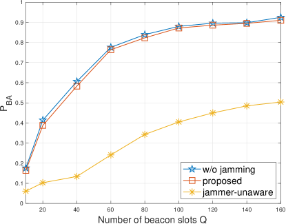
Figure 5: $P_{\text{BA}}$ versus number of beacon slots $Q$ (Case 1, $\gamma_{\text{B}}=\gamma_{\text{J}}=1$, and $\text{SJR}=-5$ dB).

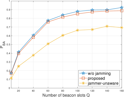
Figure 6: $P_{\text{BA}}$ versus number of beacon slots $Q$ (Case 2, $\gamma_{\text{B}}=\gamma_{\text{J}}=1$, and $\text{SJR}=-5$ dB).

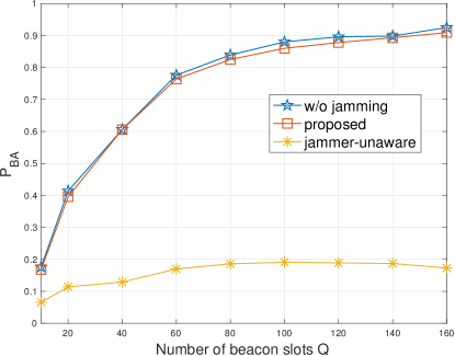
Figure 7: $P_{\text{BA}}$ versus number of beacon slots $Q$ (Case 3, $\gamma_{\text{B}}=\gamma_{\text{J}}=1$, and $\text{SJR}=-5$ dB).

VI Conclusions and directions for future work

We studied the problem of launching a jamming attack during the BA phase between the BS and users that wish to access the 5G MMW network. The considered jammer is smart in the sense that it is able to exploit the same spatial time-frequency resources that are publicly known to be used by the BS. In this case, a jamming-unaware approach is not able to ensure successful BA between the BS and the legitimate user. We proposed a novel BA procedure based on randomized probing and jammer cancellation, which guarantees performance very close to that achieved in the absence of a jamming attack.

An interesting research subject consists of considering a smart jammer that is able to modify the attack pattern according to the transmission features of the targeted communication links. For instance, the jammer might acquire information regarding the partition of each beacon slot and it may exploits such a knowledge to degrade the power estimation process in Step 2. In this case, robust solutions have to be developed that allow to adaptively reconfigure beacon partition and/or to use more advanced interference cancellation techniques, e.g., independent component analysis.

Several conditions on ${\mathbf{G}}_{\text{B}}$ are known to ensure that the sparse vector $\boldsymbol{\xi}_{\text{B}}$ can be estimated from the measurement vector ${\mathbf{p}}$. In general, the NNLS problem (37) can be ill-posed if the condition

$$\exists\boldsymbol{\alpha}\in\mathbb{R}^{\widetilde{M}\widetilde{N}_{\text{U}}Q} {\mathbf{G}}_{\text{B}}^{\text{T}}\,\boldsymbol{\alpha}>{\mathbf{0}}_{M_{\text{B}}N_{\text{U}}}$$ such that (64)

does not hold (see, e.g., [44]). Condition (64) requires the columns of ${\mathbf{G}}_{\text{B}}$ be contained in the interior of a half-space containing the origin. Such a condition is fulfilled by the transmit beamforming codebook (24).

Let $\boldsymbol{\beta}\in\mathbb{R}^{M_{\text{B}}N_{\text{U}}}$ and $\mathcal{N}\subset\{1,2,\ldots,M_{\text{B}}N_{\text{U}}\}$ be a subset. We denote with $\boldsymbol{\beta}_{\mathcal{N}}\in\mathbb{R}^{M_{\text{B}}N_{\text{U}}}$ the restriction of $\boldsymbol{\beta}$ to $\mathcal{N}$, i.e., $\{\boldsymbol{\beta}_{\mathcal{N}}\}_{n}=\{\boldsymbol{\beta}\}_{n}$ for $n\in\mathcal{N}$ and $\{\boldsymbol{\beta}_{\mathcal{N}}\}_{n}=0$ otherwise. The matrix ${\mathbf{G}}_{\text{B}}$ is said [46, Def. 4.21] to satisfy the $\ell_{2}$-robust nullspace property of order $\kappa_{\text{B}}$ with parameters $\rho\in(0,1)$ and $\varsigma>0$ if

$$\|\boldsymbol{\beta}_{\mathcal{N}}\|_{2}\leq\frac{\rho}{\sqrt{\kappa_{\text{B}}}}\,\|\boldsymbol{\beta}_{\overline{\mathcal{N}}}\|_{1}+\varsigma\,\|{\mathbf{G}}_{\text{B}}\,\boldsymbol{\beta}\|_{2}\quad\forall\boldsymbol{\beta}\in\mathbb{R}^{M_{\text{B}}N_{\text{U}}}$$ (65)

for any subset $\mathcal{N}\subset\{1,2,\ldots,M_{\text{B}}N_{\text{U}}\}$ with $|\mathcal{N}|\leq\kappa_{\text{B}}$, where $\overline{\mathcal{N}}$ is the complement of $\mathcal{N}$ in $\{1,2,\ldots,M_{\text{B}}N_{\text{U}}\}$. Property (65) implies that no $\kappa_{\text{B}}$-sparse vectors lie in the nullspace of ${\mathbf{G}}_{\text{B}}$. It is readily seen from (24) and (36) that a (nonzero) vector $\boldsymbol{\beta}\in\mathbb{R}^{M_{\text{B}}N_{\text{U}}}$ does not belong to the nullspace of ${\mathbf{G}}_{\text{B}}$ if and only if $\left({\mathbf{1}}_{\mathcal{U}_{\text{B}}^{(i)}(\widetilde{s})}\otimes{\mathbf{1}}_{\mathcal{V}^{(j)}(\widetilde{s})}\right)^{\text{T}}\boldsymbol{\beta}\neq 0$ or, equivalently,

$$\sum_{n\in\text{supp}\left({\mathbf{1}}_{\mathcal{U}_{\text{B}}^{(i)}(\widetilde{s})}\otimes{\mathbf{1}}_{\mathcal{V}^{(j)}(\widetilde{s})}\right)}\{\boldsymbol{\beta}\}_{n}\neq 0$$ (66)

for at least one $i\in\{1,2,\ldots,\widetilde{M}\}$, $j\in\{1,2,\ldots,\widetilde{N}_{\text{U}}\}$, and $\widetilde{s}\in\{0,1,\ldots,Q-1\}$. This condition is fulfilled with overwhelming probability for a $\kappa_{\text{B}}$-sparse vector $\boldsymbol{\beta}$. We refer to [47] for a rigorous proof in the case of $0/1$-Bernoulli matrices.

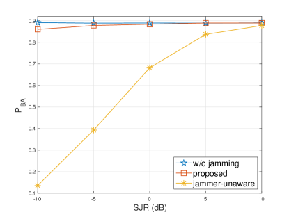
Figure 8: $P_{\text{BA}}$ versus SJR (Case 1, $\gamma_{\text{B}}=\gamma_{\text{J}}=1$, and $Q=100$).

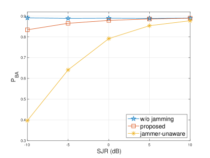
Figure 9: $P_{\text{BA}}$ versus SJR (Case 2, $\gamma_{\text{B}}=\gamma_{\text{J}}=1$, and $Q=100$).

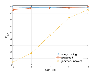
Figure 10: $P_{\text{BA}}$ versus SJR (Case 3, $\gamma_{\text{B}}=\gamma_{\text{J}}=1$, and $Q=100$).

Donatella Darsena (M’06-SM’16) received the Dr. Eng. degree summa cum laude in telecommunications engineering in 2001, and the Ph.D. degree in electronic and telecommunications engineering in 2005, both from the University of Napoli Federico II, Italy. From 2001 to 2002, she worked as embedded system designer in the Telecommunications, Peripherals and Automotive Group, STMicroelectronics, Milano, Italy. Since March 2005, she has been with the University of Napoli Parthenope, Italy. She first served as an Assistant Professor of probability theory and, since January 2022, she has served as an Associate Professor of telecommunications with the Department of Engineering. Her research interests are in the broad area of signal processing for communications, with current emphasis on backscattering communications, space-time techniques for cooperative and cognitive networks, green communications for IoT. Dr. Darsena was an Associate Editor for the IEEE COMMUNICATIONS LETTERS from December 2016 to July 2019. She has served as Associate Editor for IEEE ACCESS since October 2018, Senior Area Editor for IEEE COMMUNICATIONS LETTERS since August 2019, and Associate Editor for IEEE SIGNAL PROCESSING LETTERS since 2020.

Francesco Verde (M’10-SM’14) was born in Santa Maria Capua Vetere, Italy, on June 12, 1974. He received the Dr. Eng. degree summa cum laude in electronic engineering from the Second University of Napoli, Italy, in 1998, and the Ph.D. degree in information engineering from the University of Napoli Federico II, in 2002. Since December 2002, he has been with the University of Napoli Federico II, Italy. He first served as an Assistant Professor of signal theory and mobile communications and, since December 2011, he has served as an Associate Professor of telecommunications with the Department of Electrical Engineering and Information Technology. His research activities include reflected-power communications, orthogonal/non-orthogonal multiple-access techniques, wireless systems optimization, and physical-layer security. Prof. Verde has been involved in several technical program committees of major IEEE conferences in signal processing and wireless communications. He has served as Associate Editor for IEEE TRANSACTIONS ON COMMUNICATIONS since 2017 and Senior Area Editor of the IEEE SIGNAL PROCESSING LETTERS since 2018. He was an Associate Editor of the IEEE TRANSACTIONS ON SIGNAL PROCESSING (from 2010 to 2014) and IEEE SIGNAL PROCESSING LETTERS (from 2014 to 2018), as well as Guest Editor of the EURASIP Journal on Advances in Signal Processing in 2010 and SENSORS MDPI in 2018-2022.

References

- [1] 3GPP TS 38.104 (2019), “NR; Base Station (BS) Radio Transmission and Reception (Release 15)”, V15-6.0 (2019-6).
- [2] 3GPP TR 21.916 (2019), “Release 16 Description; Summary of Rel-16 Work Items (Release 16)”, V0.2.0 (2019-12).
- [3] T.S. Rappaport et al., “Millimeter wave mobile communications for 5G cellular: It will work!”, IEEE Access, vol. 1, pp. 335-349, May 2013.
- [4] A. Paulraj, R. Nabar, and D. Gore, Introduction to Space-Time Wireless Communications. Cambridge University Press, 2003.
- [5] D. Darsena, G. Gelli, and F. Verde, “Beamforming and precoding techniques,” Wiley 5G Ref: The Essential 5G Reference Online, 2020.
- [6] 3GPP TR 38.912 (2018), “Study on New Radio (NR) access technology (Release 15)”, V15.0.0 (2018-06).
- [7] T. Nitsche, C. Cordeiro, A.B. Flores, E.W. Knightly, E. Perahia, and J.C. Widmer, “IEEE 802.11 ad: Directional 60 GHz communication for multi-gigabit-per-second Wi-Fi,” IEEE Commun. Mag., vol. 52, pp. 132-141, Dec. 2014.
- [8] J. Wang et al., “Beam codebook based beamforming protocol for multi- Gbps millimeter-wave WPAN systems,” IEEE J. Select. Areas Commun., vol. 27, pp. 1390-1399, Oct. 2009.
- [9] S. Hur, T. Kim, D.J. Love, J.V. Krogmeier, T.A. Thomas, and A. Ghosh, “Millimeter wave beamforming for wireless backhaul and access in small cell networks,” IEEE Trans. Commun., vol. 61, pp. 4391-4403, Oct. 2013.
- [10] M. Kokshoorn, H. Chen, P. Wang, Y. Li, and B. Vucetic, “Millimeter wave MIMO channel estimation using overlapped beam patterns and rate adaptation,”IEEE Trans. Signal Process., vol. 65, pp. 601-616, Feb. 2017.
- [11] X. Song, S. Haghighatshoar, and G. Caire, “A scalable and statistically robust beam alignment technique for millimeter-wave systems,” IEEE Trans. Wireless Commun., vol. 17, pp. 4792-4805, July 2018.
- [12] M. Giordani, M. Polese, A. Roy, D. Castor, and M. Zorzi, “A tutorial on beam management for 3GPP NR at mmwave frequencies,” IEEE Commun. Surv. Tutor., vol. 21, pp. 173-196, First Quarter 2019.
- [13] N.J. Myers, A. Mezghani, and R.W. Heath, “Swift-link: A compressive beam alignment algorithm for practical mmWave radios,” IEEE Trans. Signal Process., vol. 67, pp. 1104-1119, Feb. 2019.
- [14] M. Hussain and N. Michelusi, “Energy-efficient interactive beam alignment for millimeter-wave networks,” IEEE Trans. Wireless Commun., vol. 18, pp. 838-851, Feb. 2019.
- [15] D. Zhang, A. Li, M. Shirvanimoghaddam, Y. Li, and B. Vucetic, “Exploring AoA/AoD dynamics in beam alignment of mobile millimeter wave MIMO systems,” IEEE Trans. Veh. Technol., vol. 68, pp. 6172-6176, June 2019.
- [16] M. Li, C. Liu, S.V. Hanly, I.B. Collings, and P. Whiting, “Explore and eliminate: Optimized two-stage search for millimeter-wave beam alignment,” IEEE Trans. Wireless Commun., vol. 18, pp. 4379-4393, Sept2̇019.
- [17] V. Suresh and D.J. Love, “Single-bit millimeter wave beam alignment using error control sounding strategies,” IEEE J. Select. Topics Signal Process., vol. 13, pp. 1032-1045, Sept. 2019.
- [18] X. Li, J. Fang, H. Duan, Z. Chen, and H. Li, “Fast beam alignment for millimeter wave communications: A sparse encoding and phaseless decoding approach,” IEEE Trans. Signal Process., vol. 67, pp. 4402-4417, Sept. 2019.
- [19] M. Morales-Céspedes, O.A. Dobre, and A. García-Armada, “Semi-blind interference aligned NOMA for downlink MU-MISO systems,” IEEE Trans. Commun., vol. 68, pp. 1852-1865, Mar. 2020.
- [20] C. Liu, M. Li, L. Zhao, P. Whiting, S.V. Hanly and I.B. Collings, “Millimeter-wave beam search with iterative deactivation and beam shifting,” IEEE Trans. Wireless Commun., vol. 19, pp. 5117-5131, Aug. 2020.
- [21] R. Gupta, K. Lakshmanan, and A.K. Sah, “Beam alignment for mmWave using non-stationary bandits,” IEEE Commun. Lett., vol. 24, pp. 2619-2622, Nov. 2020.
- [22] I. Chafaa, E.V. Belmega, and M. Debbah, “One-bit feedback exponential learning for beam alignment in mobile mmWave,” IEEE Access, vol. 8, pp. 194575-194589, 2020.
- [23] H. Echigo, Y. Cao, M. Bouazizi, and T. Ohtsuki, “A deep learning-based low overhead beam selection in mmWave communications,” IEEE Trans. Veh. Technol., vol. 70, pp. 682-691, Jan. 2021.
- [24] M. Wang, C. Zhang, X. Chen, and S. Tang, “Performance analysis of millimeter wave wireless power transfer with imperfect beam alignment,” IEEE Trans. Veh. Technol., vol. 70, pp. 2605-2618, Mar. 2021.
- [25] J. Zhang and C. Masouros, “Learning-based predictive transmitter-receiver beam alignment in millimeter wave fixed wireless access links,” IEEE Trans. Signal Process., vol. 69, pp. 3268-3282, 2021.
- [26] J. Zhang et al., “Joint beam training and data transmission design for covert millimeter-wave communication,”IEEE Trans. Inf. Foren. Sec., vol. 16, pp. 2232-2245, 2021.
- [27] M. Akdeniz, Y. Liu, S. Sun, S. Rangan, T. Rappaport, and E. Erkip, “Millimeter wave channel modeling and cellular capacity evaluation,” IEEE J. Select. Areas Commun., vol. 32, pp. 1164-1179, June 2014.
- [28] A.F. Molisch, V.V. Ratnam, S. Han, Z. Li, S.L.H. Nguyen, L. Li, and K. Haneda, “Hybrid Beamforming for Massive MIMO,” IEEE Commun. Magazine, vol. 55, pp. 134-141, Sept. 2017.
- [29] Z. Lu, W. Wang, and C. Wang, “Modeling, evaluation and detection of Jamming attacks in time-critical wireless applications,” IEEE Trans. Mobile Comput., vol. 13, pp. 1746-1759, Aug. 2014.
- [30] B. Sirkeci-Mergen and A. Scaglione, “Randomized space-time coding for distributed cooperative communication,” IEEE Trans. Signal Process., vol. 55, pp. 5003-5017, Oct. 2007.
- [31] L. Zhang, P.N. Suganthan, “A survey of randomized algorithms for training neural networks,” Information Sciences, vol. 364-365, pp. 146-155, Oct. 2016.
- [32] J.K. Tugnait, “Pilot spoofing attack detection and sountermeasure,” IEEE Trans. Commun., vol. 66, pp. 2093-2106, May 2018.
- [33] K. Pelechrinis, M. Iliofotou, and S.V. Krishnamurthy, “Denial of service attacks in wireless networks: The Case of jammers,” IEEE Commun. Surveys & Tutorials, vol. 13, pp. 245-57, 2011.
- [34] “Radio noise”, Recommendation ITU-R P.372-13, Sep. 2016.
- [35] R.A. Horn and C.R. Johnson, Matrix Analysis. New York: Cambridge Univ. Press, 1990.
- [36] A. M. Sayeed, “Deconstructing multiantenna fading channels,” IEEE Trans. Signal Process., vol. 50, pp. 2563-79, 2002.
- [37] R. W. Heath Jr., N. Gonzàlez-Prelcic, S. Rangan, W. Roh, and A.M. Sayeed, “An overview of signal processing techniques for millimeter wave MIMO systems,” IEEE J. Select. Areas Commun., vol. 10, pp. 436-53, 2016.
- [38] W. U. Bajwa, J. Haupt, A. M. Sayeed, and R. Nowak, “A new approach to estimating sparse multipath channels,” Proc. IEEE, vol. 98, pp. 1058-76, 2010.
- [39] J. W. Brewer, “Kronecker products and matrix calculus in system theory,” IEEE Transactions on circuits and systems, vol. CAS-25, pp. 772-81, 1978.
- [40] M.R. Akdeniz et al., “Millimeter wave channel modeling and cellular capacity evaluation,” IEEE J. Select. Areas Commun., vol. 32, pp. 1164-1179, June 2014.
- [41] A. Alkhateeb, O. El Ayach, G. Leus, and R.W. Heath, “Channel estimation and hybrid precoding for millimeter wave cellular systems,” IEEE J. Select. Topics Signal Process., vol. 8, pp. 831–846, Oct. 2014.
- [42] K. Venugopal, A. Alkhateeb, N.G. Prelcic, and R.W. Heath, “Channel estimation for hybrid architecture based wideband millimeter wave systems,” IEEE J. Select. Areas Commun., vol. 35, pp. 1996-2009, Sep. 2017.
- [43] D. Kim, S. Sra, and I. Dhillon, “Tackling box-constrained convex opti- mization via a new projected quasi-Newton approach,” SIAM Journal on Scientific Computing, vol. 32, pp. 3548-3563, 2010.
- [44] M. Slawski and M. Hein, “Non-negative least squares for high-dimensional linear models: Consistency and sparse recovery without regularization,” Electron. J. Statist., vol. 7, pp. 3004-3056, 2013.
- [45] A. Björck, Numerical Methods for Least Squares Problems. SIAM: Philadelphia, PA, 1996.
- [46] S. Foucart and H. Rauhut, A Mathematical Introduction to Compressive Sensing. Springer Science+Business Media New York 2013.
- [47] R. Kueng and P. Jung, “Robust nonnegative sparse recovery and the nullspace property of measurements,” IEEE Trans. Inf. Theory, vol. 64, pp. 689-703, Feb. 2018.
- [48] P. Frenger, P. Moberg, J. Malmodin, Y. Jading, and I. Godor, “Reducing energy consumption in LTE with cell DTX,” Proc. of 2011 IEEE 73rd Vehicular Technology Conference (VTC Spring), 2011, pp. 1-5.
- [49] A. Zaidi, F. Athley, and J. Medbo, 5G Physical Layer: Principles, Models and Technology Components. Elsevier Science Publishing Co Inc, 2018 .