A micromagnetic theory of skyrmion lifetime in ultrathin ferromagnetic films

Abstract

We use the continuum micromagnetic framework to derive the formulas for compact skyrmion lifetime due to thermal noise in ultrathin ferromagnetic films with relatively weak interfacial Dzyaloshinskii-Moriya interaction. In the absence of a saddle point connecting the skyrmion solution to the ferromagnetic state, we interpret the skyrmion collapse event as “capture by an absorber” at microscale. This yields an explicit Arrhenius collapse rate with both the barrier height and the prefactor as functions of all the material parameters, as well as the dynamical paths to collapse.

Introduction.

Magnetic skyrmions are a characteristic example of topological solitons existing at nanoscale. Their extensive studies in the past ten years revealed a very rich underlying physics as well as potential applications in the field of spintronics Kiselev et al. (2011); Nagaosa and Tokura (2013); Fert et al. (2017); Zhang et al. (2020). While the fundamental object for applications is an individual skyrmion in a homogeneous ferromagnetic environment, for topological reasons it cannot be created or annihilated by a continuous transformation from the ferromagnetic state. This transition is however enabled by the discrete nature of the condensed matter as observed experimentally Sampaio et al. (2013); Romming et al. (2013); Hagemeister et al. (2015); Wild et al. (2017).

The detailed physical mechanisms of skyrmion annihilation have been investigated at the nanoscale using atomic spin simulations combined with methods of finding the minimum energy path and harmonic transition state theory Bessarab et al. (2015); Lobanov et al. (2016); Cortés-Ortuño et al. (2017); Bessarab et al. (2018); Desplat et al. (2018); Heil et al. (2019); Lobanov et al. (2021). In particular, the energy barrier $\Delta E$ separating the skyrmion state from the ferromagnetic state was obtained numerically for some given sets of parameters and the skyrmion annihilation rate was estimated by a simple Arrhenius law $\Gamma_{0}e^{-\Delta E/(k_{B}T)}$, where $\Gamma_{0}$ is the rate prefactor, also called the attempt frequency. While early works used standard values of $\Gamma_{0}$ which are in the range from $10^{9}$ to $10^{12}$ Hz in the macrospin model Brown (1963), more recent studies show that in the case of skyrmions $\Gamma_{0}$ can vary by many orders of magnitude Wild et al. (2017); von Malottki et al. (2019); Desplat et al. (2020); Hoffmann et al. (2020).

Despite this progress, there are limitations to the atomistic simulations. First, they are computationally expensive, which limits the accessible skyrmion sizes (usually below 5 nm in diameter) and the physical parameter ranges that can be explored. Second, the obtained results depend on the microscopic details that are not necessarily known or controlled in the case of nanocrystalline systems. Under these circumstances, there is clearly a need for a more coarse-grained theory that would provide universal relations between the skyrmion lifetime and the material parameters. Moreover, it is reasonable to expect that under many physically relevant conditions the microscopic details do not play a dominant role for fluctuation-driven skyrmion collapse. For example, the skyrmion size is often much larger than the atomic lattice spacing when it loses its topological protection via the disappearance of its core Verga (2014); Heil et al. (2019).

In this Letter, we develop a theory of skyrmion lifetime based on the continuum field theory and derive the expressions for both the energy barrier and the attempt frequency as functions of all the material parameters. Starting with the stochastic Landau-Lifshitz-Gilbert partial differential equation, we first derive several integral identities associated with the fundamental continuous symmetry groups of the exchange energy. Then, in the exchange dominated regime, we carry out a finite-dimensional reduction of the stochastic skyrmion dynamics and obtain a system of stochastic ordinary differential equations for the skyrmion radius and angle. Finally, in the small thermal noise regime we use the obtained equations to calculate the Arrhenius rate, including the prefactor, by interpreting the skyrmion collapse event as “capture by an absorber” for the skyrmion radius at the atomic scale.

Model.

At the continuum level the magnetization dynamics in an ultrathin ferromagnetic film at finite temperature is described by the stochastic Landau-Lifshitz-Gilbert (sLLG) equation Landau and Lifshitz (1984); García-Cervera (2007); Brown (1963); García-Palacios and Lázaro (1998) (for the technical details on all the formulas in the paper, see sup )

$$\frac{\partial\mathbf{m}}{\partial t}=-\mathbf{m}\times\mathbf{h}_{\rm{eff}}+{\alpha}\mathbf{m}\times\frac{\partial\mathbf{m}}{\partial t},$$ (1)

where $\mathbf{m}=\mathbf{m}(\mathbf{r},t)$ is the unit magnetization vector at position $\mathbf{r}\in\mathbb{R}^{2}$ measured in the units of the exchange length $\ell_{ex}=\sqrt{2A/(\mu_{0}M_{s}^{2})}$, where $A$ is the exchange stiffness, $M_{s}$ is the saturation magnetization and $\mu_{0}$ is vacuum permeability, and time $t$ measured in the units of $\tau_{0}=(\gamma\mu_{0}M_{s})^{-1}$, where $\gamma$ is the gyromagnetic ratio, $\alpha$ is the dimensionless Gilbert damping parameter, and $\mathbf{h}_{\rm{eff}}=\mathbf{h}_{\rm{eff}}(\mathbf{r},t)\in\mathbb{R}^{3}$ is the effective field given by

$$\mathbf{h}_{\rm{eff}}=-\frac{\delta E(\mathbf{m})}{\delta\mathbf{m}}+\sqrt{2\alpha\varepsilon}\,\boldsymbol{\xi},$$ (2)

where $E(\mathbf{m})$ is the micromagnetic energy measured in the units of $2Ad$, with $d$ being the film thickness, and $\boldsymbol{\xi}=\boldsymbol{\xi}(\mathbf{r},t)\in\mathbb{R}^{3}$ is a suitable regularization of a three-dimensional delta-correlated spatiotemporal white noise Da Prato and Zabczyk (1992). In the local approximation for the stray field and in the absence of the applied field we have Bogdanov and Yablonskii (1989); Bogdanov and Hubert (1994); Thiaville et al. (2012); Muratov and Slastikov (2017); Bernand-Mantel et al. (2020, 2021)

$$E(\mathbf{m})\!=\!\frac{1}{2}\!\int_{\mathbb{R}^{2}}\!\Big{\{}|\nabla\mathbf{m}|^{2}\!+\!(Q-1)|\mathbf{m}_{\perp}|^{2}\!-\!2\kappa\mathbf{m}_{\perp}\!\cdot\!\nabla m_{\parallel}\!\Big{\}}d^{2}r,$$ (3)

which consists of, in order of appearance, the exchange, the effective uniaxial out-of-plane anisotropy ($Q>1$) and the interfacial Dzyaloshinskii-Moriya interaction (DMI) terms, respectively. Above we defined $\mathbf{m}_{\perp}\in\mathbb{R}^{2}$ and $m_{\parallel}\in\mathbb{R}$ to be the respective in-plane and out-of-plane components of the magnetization vector $\mathbf{m}=(\mathbf{m}_{\perp},m_{\parallel})$, and introduced

$$Q={2K\over\mu_{0}M_{s}^{2}},\qquad\kappa=D\sqrt{2\over\mu_{0}M_{s}^{2}A},\qquad\varepsilon={k_{B}T\over 2Ad},$$ (4)

where $K$ is the magnetocrystalline uniaxial anisotropy constant, $D$ is the DMI constant and $k_{B}T$ is temperature in the energy units. The dimensionless parameters in (4) characterize the anisotropy, the DMI and the noise strengths, respectively.

Integral identities.

We begin by rewriting the sLLG equation in the spherical coordinates, setting $\mathbf{m}=(\sin\theta\cos\phi,\sin\theta\sin\phi,\cos\theta)$, and express it in terms of $\theta$ and $\phi$. After some tedious algebra, we get

$$\left(\begin{array}[]{cc}\alpha&-1\\ 1&\alpha\end{array}\right)\left(\begin{array}[]{c}\theta_{t}\\ \sin\theta\phi_{t}\end{array}\right)=\left(\begin{array}[]{c}\Delta\theta-\sin\theta\cos\theta|\nabla\phi|^{2}-(Q-1)\cos\theta\sin\theta+\kappa\,\sin^{2}\theta\nabla\phi\cdot\mathbf{p}+\sqrt{2\alpha\varepsilon}\,\eta\\ \sin\theta\Delta\phi+2\cos\theta\nabla\theta\cdot\nabla\phi-\kappa\sin\theta\nabla\theta\cdot\mathbf{p}+\sqrt{2\alpha\varepsilon}\,\zeta\end{array}\right),$$ (11)

where $\eta$ and $\zeta$ are two independent, delta-correlated spatiotemporal white noises, $\mathbf{p}=(-\sin\phi,\cos\phi)$, and here and everywhere below the letter subscripts denote partial derivatives in the respective variables.

We next derive several integral identities for the solutions of (11) that will be useful in obtaining the evolution equations for the skyrmion characteristics. These identities are closely related to the continuous symmetry groups associated with the exchange energy term, which dominates in the considered regime. We start with the group of rotations and scalar multiply (11) by $(0,\sin\theta)$. A subsequent integration over space yields

$$\!\!\int_{\mathbb{R}^{2}}\sin\theta\theta_{t}\,d^{2}r\!+\!\alpha\int_{\mathbb{R}^{2}}\sin^{2}\theta\phi_{t}\,d^{2}r\!+\!\kappa\int_{\mathbb{R}^{2}}\sin^{2}\theta\nabla\theta\!\cdot\!\mathbf{p}\,d^{2}r\\ =\sqrt{2\alpha\varepsilon}\left(\int_{\mathbb{R}^{2}}\sin^{2}\theta\,d^{2}r\right)^{1/2}\dot{W}_{1}(t),$$ (12)

where $W_{1}(t)$ is a Wiener process, and the dot denotes the time derivative. Here we noted that an integral of a divergence term vanishes for the profiles that approach a constant vector at infinity.

Now we use the group of dilations and scalar multiply (11) by $(\nabla\theta\cdot(\mathbf{r}-\mathbf{r}_{0}(t)),\sin\theta\nabla\phi\cdot(\mathbf{r}-\mathbf{r}_{0}(t)))$, where $\mathbf{r}_{0}(t)$ is arbitrary. This yields

$$\!\!-\!\int_{\mathbb{R}^{2}}\!(\mathbf{r}\!-\!\mathbf{r}_{0}(t))\!\cdot\!\nabla\theta\,\sin\theta\phi_{t}d^{2}r\!+\!\alpha\int_{\mathbb{R}^{2}}\!(\mathbf{r}\!-\!\mathbf{r}_{0}(t)\!)\!\cdot\!\nabla\theta\,\theta_{t}d^{2}r\\ \!+\!\alpha\int_{\mathbb{R}^{2}}\!\sin^{2}\theta\nabla\phi\cdot(\mathbf{r}\!-\!\mathbf{r}_{0}(t)\!)\phi_{t}d^{2}r\!+\!\int_{\mathbb{R}^{2}}\!(\mathbf{r}\!-\!\mathbf{r}_{0}(t)\!)\cdot\!\nabla\phi\,\theta_{t}\sin\theta d^{2}r\\ \!=\!\int_{\mathbb{R}^{2}}\!(\mathbf{r}\!-\!\mathbf{r}_{0}(t)\!)\!\cdot\!\nabla\theta\,(-(Q\!-\!1)\cos\theta\sin\theta\!+\!\kappa\,\sin^{2}\theta\nabla\phi\!\cdot\!\mathbf{p})d^{2}r\\ \!+\!\int_{\mathbb{R}^{2}}\!\sin\theta\nabla\phi\!\cdot\!(\mathbf{r}\!-\!\mathbf{r}_{0}(t)\!)(-\kappa\sin\theta\nabla\theta\!\cdot\!\mathbf{p})d^{2}r\\ \!+\!\sqrt{\int_{\mathbb{R}^{2}}\!|(\mathbf{r}\!-\!\mathbf{r}_{0}(t)\!)\!\cdot\!\nabla\theta|^{2}d^{2}r\!+\!\int_{\mathbb{R}^{2}}\!\sin^{2}\theta|(\mathbf{r}\!-\!\mathbf{r}_{0}(t)\!)\!\cdot\!\nabla\phi|^{2}d^{2}r}\\ \times\sqrt{2\alpha\varepsilon}\,\dot{W}_{2}(t),$$ (13)

where $W_{2}(t)$ is another Wiener process. Finally, we use the translational symmetries of the exchange energy and scalar multiply the stochastic LLG equation by $(\theta_{x},\sin\theta\phi_{x})$ or $(\theta_{y},\sin\theta\phi_{y})$ to obtain two similar identities involving two other Wiener processes $W_{3}(t)$ and $W_{4}(t)$ sup . Note that in general the Wiener processes $W_{1}(t)$ through $W_{4}(t)$ are not independent.

Reduction to a finite-dimensional system.

To proceed further, we focus on the regime in which a good approximation to the solutions of the sLLG equation may be obtained by means of a matched asymptotic expansion. This regime, in which $0<\kappa\ll\sqrt{Q-1}$ gives rise to a skyrmion profile $(\theta,\phi)=(\bar{\theta},\bar{\phi})$ whose radius $\rho_{0}$ is asymptotically Bernand-Mantel et al. (2020); Komineas et al. (2020); Bernand-Mantel et al. (2021)

$$\rho_{0}\simeq{\kappa\over 2(Q-1)\ln\left(a\kappa^{-1}\sqrt{Q-1}\right)},$$ (14)

for some $a\sim 1$. It is characterized by a compact core on the scale of $\rho_{0}$:

$$\bar{\theta}(r)\simeq 2\arctan(r/\rho_{0}),$$ (15)

which is the Belavin-Polyakov profile Belavin and Polyakov (1975) that minimizes the exchange energy at leading order, and an exponentially decaying tail on the scale of the Bloch wall length $L=(Q-1)^{-1/2}$:

$$\bar{\theta}(r)\simeq\pi-2\rho_{0}\sqrt{Q-1}\,K_{1}(r\sqrt{Q-1}),$$ (16)

where $K_{0}(z)$ is the modified Bessel function of the second kind, that minimizes the exchange plus anisotropy energy to the leading order. In both the core and the tail $\bar{\phi}=\psi-\pi$, where $x=r\cos\psi$ and $y=r\sin\psi$ are the polar coordinates relative to the skyrmion center.

Dynamically, one would expect that for $\alpha\sim 1$ the above profile would stabilize on the diffusive timescale $\tau_{\mathrm{core}}\sim\rho^{2}$ in the core, and on the relaxation timescale $\tau_{\mathrm{relax}}\sim(Q-1)^{-1}$ in the tail, respectively. Therefore, on the timescale $\tau_{\mathrm{relax}}\gtrsim\tau_{core}$ the dynamical profile $\theta(\mathbf{r},t)$ in the skyrmion core would be expected to be dominated by the exchange and, therefore, stay close to a suitably translated, rotated and dilated Belavin-Polyakov profile:

$$\theta(\mathbf{r},t) \simeq 2\arctan(|\mathbf{r}-\mathbf{r}_{0}(t)|/\rho(t)),$$ (17)

$$\phi(\mathbf{r},t) \simeq\arg(\mathbf{r}-\mathbf{r}_{0}(t))-\pi+\varphi(t).$$ (18)

Similarly, on the timescale $\gtrsim\tau_{\mathrm{relax}}$ the skyrmion profile in the tail should approach

$$\theta(\mathbf{r},t)\simeq\pi-2\rho(t)\sqrt{Q-1}\,K_{1}(|\mathbf{r}-\mathbf{r}_{0}(t)|\sqrt{Q-1}).$$ (19)

Here, the functions $\rho(t)$, $\varphi(t)$ and $\mathbf{r}_{0}(t)$ may be interpreted, respectively, as the instantaneous radius, rotation angle and the center of the skyrmion.

The above approximate solution may be substituted into our integral identities to obtain a closed set of equations for $\rho(t)$, $\varphi(t)$ and $\mathbf{r}_{0}(t)=(x_{0}(t),y_{0}(t))$:

$$\!\!\!{d\over dt}\left(\begin{array}[]{c}\ln\rho\\ \varphi\end{array}\right)=-{1\over 1+\alpha^{2}}\left(\begin{array}[]{cc}\alpha&-1\\ 1&\alpha\end{array}\right)\left(\begin{array}[]{c}Q-1-{\kappa\cos\varphi\over 2\rho\ln(L/\rho)}\\ {\kappa\sin\varphi\over 2\rho\ln(L/\rho)}\end{array}\right)\\ +\sqrt{\alpha\varepsilon\over 4\pi(1+\alpha^{2})\rho^{2}\ln(L/\rho)}\left(\begin{array}[]{c}\dot{W}_{1}(t)\\ \dot{W}_{2}(t)\end{array}\right),$$ (20)

and

$$\dot{x}_{0}=\sqrt{\alpha\varepsilon\over 2\pi(1+\alpha^{2})}\,\dot{W}_{3},\quad\dot{y}_{0}=\sqrt{\alpha\varepsilon\over 2\pi(1+\alpha^{2})}\,\dot{W}_{4}.$$ (21)

Furthermore, to the leading order the Wiener processes $W_{1}(t)$ through $W_{4}(t)$ are all mutually independent. It is understood that $\rho$ is bounded above by some $L_{0}<L$. Moreover, when $\rho\sim\rho_{0}$, we may set the large logarithmic factor $\ln(L/\rho)$ to a constant $\Lambda=\ln(a\kappa^{-1}\sqrt{Q-1})$ to the leading order. Introducing the new variable $\bar{z}=\bar{x}+i\bar{y}=\rho e^{i\varphi}$ then results in the following stochastic differential equation:

$$d\bar{z}(t)=-{\alpha+i\over 1+\alpha^{2}}\left[(Q-1)\bar{z}(t)-{\kappa\over 2\Lambda}\right]dt$$

$$+\sqrt{\alpha\varepsilon\over 4\pi\Lambda(1+\alpha^{2})}\,d\bar{W}(t),$$ (22)

where $\bar{W}(t)=W_{1}(t)+iW_{2}(t)$ is a complex-valued Wiener process. Note that the dynamics of $\bar{z}(t)$ decouples from that of $\mathbf{r}_{0}(t)$, with the latter undergoing a simple diffusion with diffusivity $D_{\mathrm{eff}}={\alpha\varepsilon\over 4\pi(1+\alpha^{2})}$, in agreement with Schütte et al. (2014).

Calculation of the collapse rate.

We now focus on the analysis of (Reduction to a finite-dimensional system.). It describes a two-dimensional shifted Ornstein-Uhlenbeck process, whose equilibrium measure is given by the Boltzmann distribution

$$p_{\mathrm{eq}}(\bar{z})={4\Lambda\varepsilon^{-1}(Q-1)}e^{-{H(\bar{z})\over\varepsilon}},$$ (23)

where

$$H(\bar{z})=4\pi\Lambda(Q-1)|\bar{z}-\bar{z}_{0}|^{2},\quad\bar{z}_{0}={\kappa\over 2\Lambda(Q-1)},$$ (24)

which is peaked around $\bar{z}=\bar{z}_{0}$ in the complex plane. This distribution is attained on the timescale of $\tau_{\mathrm{relax}}$.

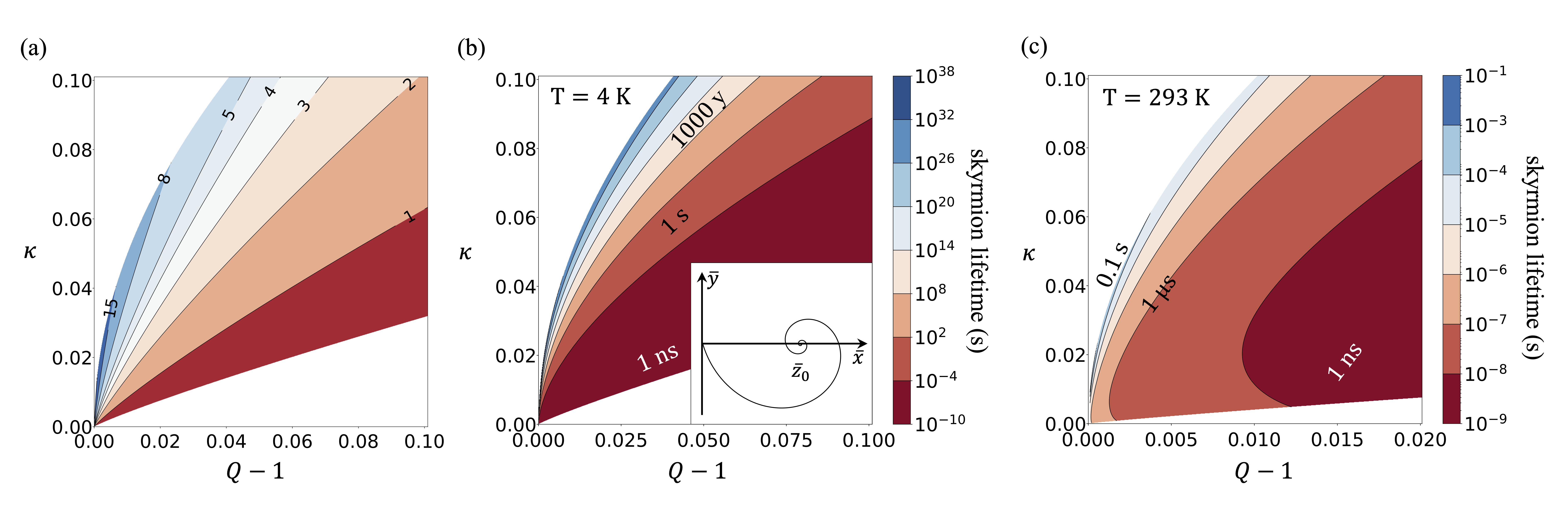
Figure 1: (a) Skyrmion equilibrium radius $\ell_{\mathrm{ex}}\rho_{0}$ in nm, with $\ell_{\mathrm{ex}}=8.4$ nm and $\rho_{0}$ from (14). (b) and (c) Skyrmion lifetime $\tau_{0}/J_{\delta}$ for $\tau_{0}=7.8\times 10^{-12}$ s, $\alpha=0.3$, $\delta=0.0475$, with $J_{\delta}$ from (29) for $\varepsilon=0.0046$ ($T=4$K) in (b) and $J_{\delta}$ from (32) for $\varepsilon=0.337$ ($T=293$K) in (c). In (a) and (b), only the region $\kappa/\sqrt{Q-1}<\frac{1}{2}$ is shown. Inset: The optimal collapse path $\bar{z}_{\mathrm{opt}}(t)$ from (34).

Notice that the probability of the solutions of (Reduction to a finite-dimensional system.) starting at $\bar{z}=\bar{z}_{0}$ to hit the origin is zero, although the probability to come to an arbitrarily small neighborhood of the origin is unity. Therefore, within (Reduction to a finite-dimensional system.) a more careful definition of the skyrmion collapse event is necessary. For that purpose, we note that when the skyrmion radius becomes sufficiently small, the continuum micromagnetic description of the magnetization profile breaks down. This happens when the skyrmion radius reaches the atomic scale, at which point the skyrmion loses its topological protection. Therefore, to model skyrmion collapse we supplement (Reduction to a finite-dimensional system.) with an absorbing boundary condition at $|\bar{z}|=\delta$ for some cutoff radius $\delta\ll\bar{z}_{0}$. In atomically thin films, this cutoff radius is on the order of the film thickness measured in the units of the exchange length, $\delta\sim d/\ell_{\mathrm{ex}}$. The mean skyrmion lifetime may then be found by solving an appropriate boundary value problem in the plane. When $\varepsilon\ll 1$, it may be obtained by investigating the stationary solution $p=p(\bar{x},\bar{y})$ of the Fokker-Planck equation associated with (Reduction to a finite-dimensional system.) with a suitable source $g(\bar{x},\bar{y})$ away from the absorber:

$$\left[(Q-1)x-{\kappa\over 2\Lambda}\right](\alpha q_{\bar{x}}-q_{\bar{y}})+y(Q-1)(\alpha q_{\bar{y}}+q_{\bar{x}})$$

$$={\alpha\varepsilon\over 8\pi\Lambda}(q_{\bar{x}\bar{x}}+q_{\bar{y}\bar{y}})+gp_{\mathrm{eq}}^{-1},$$ (25)

where we introduced $q=p/p_{\mathrm{eq}}$ and set $q=0$ at $|\bar{z}|=\delta$. When $\varepsilon\to 0$, we are interested in the boundary layer solution of (25) in the neighborhood of $(\bar{x},\bar{y})=(\delta,0)$, in which the probability flux is concentrated Gardiner (1997). The function $q$ approaches 1 away from the boundary layer. Then to the leading order in $\varepsilon$, the solution in a small neighborhood around the point $(\bar{x},\bar{y})=(\delta,0)$ is given by

$$q(\bar{x},\bar{y})\simeq 1-\exp\left\{-{8\pi\Lambda\over\varepsilon}\left[(Q-1)\delta-{\kappa\over 2\Lambda}\right](\bar{x}-\delta)\right\}.$$ (26)

Assuming that $\varepsilon\ll\kappa\delta$, the corresponding total probability flux into the boundary is, to the leading order,

$$J_{\delta}={\alpha\varepsilon\over 8\pi\Lambda(1+\alpha^{2})}\int_{|\bar{z}|=\delta}p_{\mathrm{eq}}|\nabla q|\,ds$$ (27)

$$\simeq{\alpha\Lambda(Q-1)\over 1+\alpha^{2}}\left[{\kappa\over 2\Lambda}-(Q-1)\delta\right]\left({8\delta\over\varepsilon\kappa}\right)^{1/2}\,e^{-{H(\delta)\over\varepsilon}},$$ (28)

which has the form of an Arrhenius law with explicit expressions for the barrier height $H(\delta)$ and the prefactor. Notice that the latter depends weakly on the parameter $\delta\ll 1$, and to the leading order we have

$$J_{\delta}\simeq{\alpha(Q-1)A_{\delta}\over 1+\alpha^{2}}\left({2\kappa\delta\over\varepsilon}\right)^{1/2}\exp\left\{{-{\pi\kappa^{2}\over\varepsilon\Lambda(Q-1)}}\right\},$$ (29)

where $\pi\kappa^{2}/[\Lambda(Q-1)]$ is the leading order barrier height $H(0)$ and

$$A_{\delta}=\exp\left\{{4\pi\kappa\delta\over\varepsilon}\left[1-{\Lambda(Q-1)\delta\over\kappa}\right]\right\}>1$$ (30)

is an anomalous factor due to a small reduction $\Delta H=H(0)-H(\delta)$ of the barrier height resulting from the presence of the absorber at microscale needed to break the topological protection.

The quantity in (29) gives the leading order asymptotic skyrmion collapse rate for $\delta\ll 1$ as $\varepsilon\to 0$. The exponential term is nothing but the Arrhenius factor associated with the energy barrier to collapse, to the leading order in $\kappa/\sqrt{Q-1}\ll 1$. A comparison with the result of the numerical solution for the radial skyrmion profile sup shows that taking $a=2.8$ in the definition of $\Lambda=\ln(a\kappa^{-1}\sqrt{Q-1})$ reproduces the exact barrier height to within 17% for all $\kappa/\sqrt{Q-1}<0.8$.

It is also possible to obtain the skyrmion collapse rate in the limit $\delta\to 0$ with $\varepsilon\ll 1$ and all the other parameters fixed, corresponding to the opposite extreme $\varepsilon\gg\kappa\delta$. Here in the $O(\varepsilon/\kappa)$ neighborhood of the absorber the function $q(\bar{x},\bar{y})$ is, to the leading order in $\delta\ll 1$,

$$q(\bar{x},\bar{y})\simeq{\ln\left({\sqrt{\bar{x}^{2}+\bar{y}^{2}}\over\delta}\right)\over\ln\left({b\alpha\varepsilon\over\kappa\delta\sqrt{1+\alpha^{2}}}\right)},$$ (31)

where $b\approx 0.179$. An analogous computation to the one leading to (29) yields in this case

$$J_{\delta}\simeq{\alpha(Q-1)A_{\delta}\over(1+\alpha^{2})\ln\left({b\alpha\varepsilon\over\kappa\delta\sqrt{1+\alpha^{2}}}\right)}\,\exp\left\{{-{\pi\kappa^{2}\over\varepsilon\Lambda(Q-1)}}\right\}.$$ (32)

The condition $\varepsilon\gg\kappa\delta$ or, equivalently, $\delta\ll\varepsilon/\kappa$ ensures that $p_{\mathrm{eq}}(\bar{x},\bar{y})$ does not vary appreciably across the absorber boundary, making $A_{\delta}\simeq 1$ as $\delta\to 0$.

Skyrmion collapse paths.

The dynamics of skyrmion collapse in the small noise limit may be understood through the minimization of the large deviation action associated with (Reduction to a finite-dimensional system.) Freidlin and Wentzell (1998):

$$S={2\pi\Lambda(1+\alpha^{2})\over\alpha}\\ \times\int_{0}^{T}\left|\dot{\bar{z}}+{\alpha+i\over 1+\alpha^{2}}\left[(Q-1)\bar{z}-{\kappa\over 2\Lambda}\right]\right|^{2}dt.$$ (33)

Minimizing over all trajectories $\bar{z}(t)$ that start at $\bar{z}(0)=\bar{z}_{0}$ and terminate at $\bar{z}(T)=\delta$, and then sending $T\to\infty$, one obtains the optimal collapse trajectory $\bar{z}=\bar{z}_{\mathrm{opt}}(t)$, where to the leading order in $\delta\ll 1$ we have

$$\bar{z}_{\mathrm{opt}}(t)=\bar{z}_{0}\left(1-e^{{\alpha-i\over 1+\alpha^{2}}(Q-1)(t-T)}\right).$$ (34)

As expected, for $\alpha\lesssim 1$ the collapse occurs on the timescale $\alpha^{-1}(Q-1)^{-1}$ and acquires an oscillatory character for $\alpha\ll 1$. The optimal path to collapse is illustrated in the inset in Fig. 1(b). Notice that for $\alpha\ll 1$ the skyrmion angle rotates as the skyrmion radius shrinks to zero, similarly to what is observed in current-driven skyrmion collapse Verga (2014).

Parametric dependence of skyrmion lifetime.

We now use the obtained formulas for the collapse rate to calculate the skyrmion lifetimes as functions of the material parameters in a typical ultrathin ferromagnetic film. For that purpose, we take the same parameters as in Sampaio et. al. Sampaio et al. (2013): $d=0.4$ nm, $A=15$ pJ/m, $M_{s}=0.58$ MA/m, $\alpha=0.3$. This yields $\ell_{\mathrm{ex}}=8.4$ nm, $\tau_{0}=7.8\times 10^{-12}$ s and $\delta=d/\ell_{\mathrm{ex}}=0.0475$. The equilibrium skyrmion radius and lifetime $\tau_{0}/J_{\delta}$ as functions of the dimensionless parameters $Q-1$ and $\kappa$ are plotted in Fig. 1. The low temperature regime corresponding to (29) is illustrated in Fig. 1(b), while the high temperature regime corresponding to (32) is illustrated in Fig. 1(c). In both cases, the lifetime varies by many orders of magnitude, and this variation is dominated by the exponential dependence on the barrier height proportional to $\bar{\kappa}^{2}$, where $\bar{\kappa}=\kappa/\sqrt{Q-1}$ is the classical parameter which determines the transition from the ferromagnetic to the helical ground state happening at $\bar{\kappa}=4/\pi$ Bogdanov and Hubert (1994). The lifetime increases upon increase of $\bar{\kappa}$ and is maximal when $\bar{\kappa}\sim 1$, at the borderline of applicability of our analysis.

In addition to the variation of the barrier height, we also predict a variation of the effective rate prefactor. This variation is stronger in the low temperature case [Fig. 1(b)], where it is dominated by the anomalous factor $A_{\delta}$. In this regime the rate prefactor becomes strongly dependent on the reduction in the barrier height due to the microscopic processes associated with the loss of the topological protection modeled by us by an absorbing boundary condition. This strong variation of the prefactor is similar to the strong prefactor dependence on microscopic details (layer stacking, number of magnetic monolayers, etc.) observed in recent simulations Hoffmann et al. (2020). In the high temperature regime ($\varepsilon\gg\kappa\delta$), our prediction confirms that the prefactor becomes essentially independent of the microscopic details. The remaining dependence of the prefactor is dominated by its dependence on $Q-1$ due to the expected proportionality of the attempt frequency to the precession frequency $\gamma\mu_{0}M_{s}(Q-1)$ Brown (1963).

Conclusion.

To summarize, we carried out a derivation of skyrmion lifetime, using the stochastic Landau-Lifshitz-Gilbert equation within the framework of continuum micromagnetics and accounting for the loss of topological protection via an absorbing boundary condition at microscale. Our formulas in (29) and (32) provide the first relation of skyrmion collapse rate to material parameters and could be used as a guide in material system design in view of optimizing the skyrmion lifetime for applications. The methodology developed by us may also have a wide applicability to other physical systems in which a topological defect disappears through singularity formation at the continuum level.