Toward Annotator Group Bias in Crowdsourcing

Abstract

Crowdsourcing has emerged as a popular approach for collecting annotated data to train supervised machine learning models. However, annotator bias can lead to defective annotations. Though there are a few works investigating individual annotator bias, the group effects in annotators are largely overlooked. In this work, we reveal that annotators within the same demographic group tend to show consistent group bias in annotation tasks and thus we conduct an initial study on annotator group bias. We first empirically verify the existence of annotator group bias in various real-world crowdsourcing datasets. Then, we develop a novel probabilistic graphical framework GroupAnno to capture annotator group bias with a new extended Expectation Maximization (EM) training algorithm. We conduct experiments on both synthetic and real-world datasets. Experimental results demonstrate the effectiveness of our model in modeling annotator group bias in label aggregation and model learning over competitive baselines.

1 Introduction

The performance of supervised machine learning algorithms heavily relies on the quality of the annotated training data. Due to the heavy workload of annotation tasks, researchers and practitioners typically take advantage of crowdsourcing platforms to obtain cost-effective annotation data Snow et al. (2008); Buhrmester et al. (2016). However, the labels collected from multiple crowdsourcing annotators could be not consistent, since the expertise and reliability of the annotators are uncertain, and the task itself could be subjective and difficult. In recent years, a lot of efforts from the machine learning community have been conducted to mitigate the effect of these noisy crowdsourcing labels Zheng et al. (2017). Various approaches have been proposed to model the quality Liu et al. (2012); Aydin et al. (2014), confidence Joglekar et al. (2013), expertise Ma et al. (2015); Zheng et al. (2016), reliability Li et al. (2019) of annotators; or model the difficulty of the tasks Whitehill et al. (2009); Ma et al. (2015). With such information, we can infer the truth label from the noisy labels more accurately and correspondingly train a more desirable model.

In terms of annotator modeling, existing studies mainly concentrated on factors like quality, confidence, expertise, etc., which could affect the annotation results. Besides, the bias or stereotypes held by the annotators can also lead to defective annotations Sap et al. (2019), which is, however, rarely studied. In addition, the majority of these studies merely focused on the factors on each individual annotator, but didn’t consider the possible group effect in annotators. However, we observe that annotators in different demographic groups tend to show different bias in annotation tasks. For example, in a preliminary study, we examine the instances annotated by both two groups of annotators in the Wikipedia Toxicity dataset Wulczyn et al. (2017). We observe that native speakers of English rate $5.1\%$ more comments as toxic than non-native speakers. Similarly, annotators over 30 years old rate $2.5\%$ more comments as toxic than younger annotators. More details of the preliminary study can be found in Section 2. Thus, a thorough investigation on such annotator group bias is desired. Similar to existing studies, by considering the effect of annotator group bias, we have the potential to achieve a more accurate inference of true labels and train a better model. Meanwhile, it is often hard to estimate the individual bias of one annotator with limited annotation data. With annotator group bias as the prior knowledge, we can estimate the bias more effectively based on the demographic groups the annotator belongs to. Thus, annotator group bias could mitigate the “cold-start” problem in modeling the annotator individual bias.

In this paper, we aim to study how to detect annotator group bias under text classification tasks, and how to mitigate the detrimental effects of annotator group bias on model training. We face several challenges. First, given noisy annotated data without the true labels, how should we detect the annotator bias? We first make a comparison of the annotation results from different groups of annotators and find that there is a significant gap between them. Then, we use two metrics sensitivity and specificity to measure the annotator bias, and conduct an analysis of variance (ANOVA) which demonstrates that the bias of each individual annotator shows obvious group effects in terms of its demographic attributes. Second, how can we estimate the annotator group bias, and perform label aggregation and model training with the knowledge of annotator group bias? Following the traditional probabilistic approaches for label aggregation Raykar et al. (2010); Rodrigues and Pereira (2018); Li et al. (2019), we propose a novel framework GroupAnno that models the production of annotations as a stochastic process via a novel probabilistic graphical model (PGM). Inspired by the results of ANOVA, we assume that the bias of an individual annotator follows a Beta distribution with a prior subject to its demographic attributes. We thereby extend the original PGM for label aggregation with additional variables representing annotator group bias. By learning the PGM, we estimate the annotator group bias, infer the true labels, and optimize our classification model simultaneously. Third, how can we learn this PGM effectively? With the unknown true label as the latent variable, typical label aggregation models are learned by the Expectation Maximization (EM) algorithm. However, in our PGM, we introduce another latent variable to model the bias of each annotator where the vanilla EM algorithm is not applicable. To address this challenge, we propose an extended EM algorithm for GroupAnno.

We summarize our contributions in this paper as follows. First, we propose metrics to measure the annotator group bias and verify its existence in real NLP datasets via an empirical study. Second, we propose a novel framework GroupAnno to model the annotation process by considering the annotator group bias. Third, we propose a novel extended EM algorithm for GroupAnno where we estimate the annotator group bias, infer the true labels, and optimize the text classification model simultaneously. Finally, we conduct experiments on synthetic and real data. The experimental results show that GroupAnno can accurately estimate the annotator group bias. Also, compared with competitive baselines, GroupAnno can infer the true label more accurately, and learn better classification models.

2 Understanding Annotator Group Bias

In this section, we perform an empirical study to get a rudimentary understanding of annotator group bias.

2.1 Data and Tasks

We investigate the group annotator bias on three datasets that involve various text classification tasks. These datasets are released in the Wikipedia Detox project Wulczyn et al. (2017): Personal Attack Corpus, Aggression Corpus, and Toxicity Corpus where each instance is labeled by multiple annotators from the Crowdflower platform . For all the datasets, the demographic attributes of the annotators are collected. The statistics of these datasets can be found in Appendix A.

The Personal Attack dataset and the Aggression dataset contain the same comments collected from English Wikipedia. Each comment is labeled by around 10 annotators on two tasks, respectively. The task of the former dataset is to determine whether the comment contains any form of personal attack, while the task of the latter dataset is to judge whether the comment is aggressive or not. For each annotator, four demographic categories are collected: gender, age, language, and education. Although the original dataset provides more fine-grained partitions, for simplicity, we divide the annotators into only two groups in terms of each demographic category. We consider two groups: male and female for gender, under 30 and over 30 for age, below bachelor and above bachelor (including bachelor) for education, and native and non-native speaker of English for language. The toxicity dataset contains comments collected from the same source. Similarly, each comment is labeled by around 10 annotators on whether it is toxic or not. The toxicity dataset includes the same demographic information of the annotators as the former two datasets.

2.2 Empirical Study

Table 1: The positive rates of the annotations from different groups of annotators.

Dataset	Gender		Age		Education		Language
	Male	Female	Under 30	Over 30	Below Ba.	Above Ba.	Native	Non-native
PersonalAttack	15.98	18.67	15.83	18.52	17.63	15.81	19.95	14.40
Aggression	17.74	21.44	17.79	20.85	20.28	17.62	23.20	16.08
Toxicity	12.06	16.37	12.51	15.08	15.16	12.56	16.93	11.80

To investigate whether the annotators from different groups behave differently in annotation tasks, we first perform a comparison of the annotation results from different annotator groups. For each demographic category, we collect the instances which are labeled by annotators from both groups, and report the proportion of instances that are classified as positive. The results are shown in Table 1. First, we note that there are obvious gaps between the annotations given by different annotator groups. Second, given that the tasks of the three datasets are similar (i.e., all of them are related to detecting inappropriate speech), the annotation tendency of each annotator group is the same. For example, young and non-native speaker annotators are less likely to annotate a comment as attacking, aggressive, or toxic. Third, in terms of different demographic categories, the gaps between the annotations from the two groups are different. For example, compared with other group pairs, the annotations provided by native speakers and non-native speakers are more different.

Table 2: The results of analysis of variance. The table shows the inter-group sum of squares (variance of treatments). *, ** indicate that the group effects are significant at $p<0.05$ and $p<0.005$.

Category	Personal Attack		Aggression		Toxicity
	Sensitivity	Specificity	Sensitivity	Specificity	Sensitivity	Specificity.
Gender	0.010	0.077*	0.106	0.182**	0.217**	0.266**
Age	3.093**	0.257**	3.529**	0.348**	3.230**	0.348**
Education	0.006	0.001	0.021	0.012	0.012	0.013
Language	0.805**	0.155**	1.200**	0.470**	0.041	0.023*

Analysis of Variance. The results in Table 1 suggest that annotators show group bias in the annotation tasks, which is manifested in that different groups hold different evaluation criteria in the same task. Specifically for classification tasks, different annotators are unevenly likely to label instances belonging from one class to another class. In this paper, we only consider binary classification tasks for simplicity . Thus, we use sensitivity (true positive rate) and specificity (1 $-$ false positive rate) Yerushalmy (1947) to describe the bias of an individual annotator.

Next, we seek to verify the existence of annotator group bias. We are interested in whether the demographic category of an individual annotator has a significant impact on its bias. Thus, we first estimate the bias (i.e., sensitivity and specificity) of each individual annotator from its annotation data. Since we don’t have the true labels, we use majority vote labels as the true labels to approximately estimate the bias of each annotator. Then, we perform an ANOVA Scheffe (1999) with the demographic category as the factors, the groups as the treatments, and the bias of an annotator as the response variable, to analyze the significance of the annotator’s demographic groups against its own bias. The corresponding statistical model can be expressed as:

$$\tilde{\pi}_{r}=u+\pi^{1,g^{1}_{r}}+\cdots+\pi^{P,g^{P}_{r}}+\epsilon_{r}$$ (1)

where $\tilde{\pi}_{r}$ indicates the bias of an individual annotator $r$; $u$ is the average bias of all annotators; $\pi^{p,g^{p}_{r}}$ is the effect of the group $g^{p}_{r}$ in terms of category $p$; and $\epsilon_{r}$ is the random error which follows a normal distribution with the mean value as 0. To test whether category $p$ has a significant impact on $\tilde{\pi}$, we consider the null hypothesis $H_{0p}:\pi^{p,0}=\pi^{p,1}$, which indicates that the demographic category $p$ has no significant effect on the annotator bias. In other words, there is no significant difference between the annotation behaviors of the two groups in terms of category $p$.

The results are shown in Table 2. In the table, we report the inter-group sum of squares, which represent the deviation of the average group bias from the overall average bias. We also use “$*$” to denote the significance of the hypothesis tests. We observe that in categories of gender, age and language, the two opposing groups show obvious different sensitivity and specificity in most cases. Moreover, the ANOVA suggests that we are confident to reject the null hypotheses in these cases, which means that the above three demographic categories can affect the annotator bias significantly in different datasets. Based on our observations, we conclude that the demographic attribute of an annotator can have a significant impact on its annotation behavior, and thereby, annotator group bias does exist.

3 Modeling Annotator Group Bias

In this section, we discuss our approaches for annotator group bias estimation, as well as bias-aware label aggregation and model training. We first introduce the metrics for measuring annotator group bias, and then present the problem statement. Next, we detail GroupAnno, the probabilistic graphical model for modeling the production of annotations. Finally, we describe our extended EM algorithm for learning the proposed model.

3.1 Measurements

To measure the annotator bias in terms of demographic groups, we extend the definitions of sensitivity and specificity to the group scenario. Formally, we define group sensitivity and group specificity of a group $g$ in terms of category $p$ as follows

$$\alpha^{p,g} =Pr(z=1|y=1,g_{r}^{p}=g)$$

$$\beta^{p,g} =Pr(z=0|y=0,g_{r}^{p}=g)$$

where $y$ is the true label and $z$ is the annotated label. $g_{r}^{p}=g$ represents that the annotator $r$ belongs to group $g$ in terms of demographic category $p$.

We use $\pi^{p}=(\alpha^{p,0},\alpha^{p,1},\beta^{p,0},\beta^{p,1})$ to denote the bias parameters of demographic category $p$. The bias parameters of all the $P$ categories are denoted as $\pi=\{\pi^{p}\}_{p=1}^{P}$.

3.2 Problem Statement

Suppose that we have a dataset $\mathbf{D}=\{x_{i},z_{i}^{1},\cdots,z_{i}^{R_{i}}\}_{i=1}^{N}$ which contains $N$ instances. Each instance $x_{i}$ is annotated by $R_{i}$ different annotators, which results in labels $z_{i}^{1},\cdots,z_{i}^{R_{i}}$. We also have an annotator set $\mathbf{A}=\{(g_{r}^{1},\cdots,g_{r}^{P})\}_{r=1}^{R}$ that records the demographic groups of a total of $R$ annotators. Here, $g_{r}^{p}\in\{0,1\}$ indicates the group that the $r$-th annotator belongs to in terms of the $p$-th demographic category. We consider $P$ demographic categories for each annotator, and we have two groups (i.e., 0 and 1) for each category. Given $\mathbf{D}$ and $\mathbf{A}$, we seek to (1) estimate the annotator group bias $\pi$; (2) estimate the true label $y_{i}$ of each instance $x_{i}$; and (3) learn a classifier $P_{\mathbf{w}}(y|x)$ which is parameterized by $\mathbf{w}$.

Next, we introduce our GroupAnno to model the annotation process, and propose an extended EM algorithm to estimate the parameters $\Theta=\{\mathbf{w},\pi\}$.

3.3 GroupAnno: The Probabilistic Graphical Model

As shown in Figure 1, GroupAnno models the generation procedure of annotations as follows. Given an instance $x$, its true label $y$ is determined by an underlying distribution $P_{\mathbf{w}}(\cdot|x)$. The distribution is expressed via a classifier with parameters $\mathbf{w}$ that we will learn. Given the true label $y$, the annotated label $z^{r}$ from an annotator $r$ is determined by its bias $\tilde{\pi}_{r}=(\tilde{\alpha}_{r},\tilde{\beta}_{r})$ For simplicity, in the following formulations, we use $\tilde{\pi}_{r}$ to represent $\tilde{\alpha}_{r}$ or $\tilde{\beta}_{r}$. To incorporate the prior knowledge from the demographic attributes of an annotator, we assume that the annotator bias $\tilde{\pi}_{r}$ follows a Beta prior, which can naturally model the distribution of the probability of a binary event. In Section 2.2, we show that the annotator bias can be modeled by a superposition of the effects of annotator group bias with a random variable reflecting the annotator individual bias. Thus, following Eq 1, we assume that the annotator bias of annotator $r$ follows a Beta distribution $\tilde{\pi}^{r}\sim Beta(a^{r}_{1},a^{r}_{2})$, where the mean value $\mu_{r}$ is decomposed as

$$\mu_{r}=\frac{a^{r}_{1}}{a^{r}_{1}+a^{r}_{2}}=u+\pi^{1,g^{1}_{r}}+\cdots+\pi^{P,g^{P}_{r}}+\pi_{r}$$

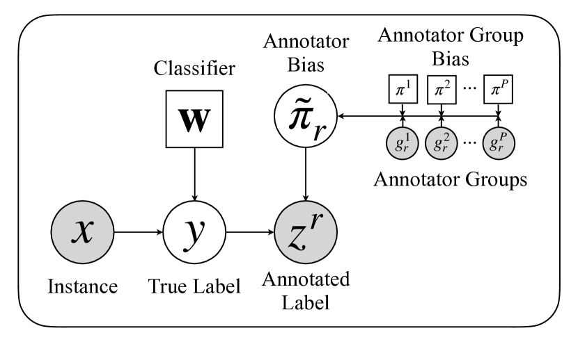
Figure 1: An illustration of GroupAnno. In the graph, grey circles represent observed data; white circles indicate latent variables; and squares denote the unknown parameters that we will learn.

To sum up, the parameters we introduced to model annotator bias are $\mathbf{\pi}=\{u\}\cup\{\pi^{p}\}_{p=1}^{P}\cup\{\pi_{r}\}_{r=1}^{R}$. To estimate the parameters $\Theta=\{\mathbf{w},\pi\}$, one way is to use maximum likelihood estimation (MLE). Under the assumption that instances are sampled independently, the likelihood function of $\Theta$ can be written as

$$P(\mathbf{D}|\mathbf{\Theta}) =\prod_{i=1}^{N}P(z_{i}^{1},\cdots,z_{i}^{R_{i}}|x_{i};\Theta)$$

Therefore, the MLE parameters can be found by maximizing the log-likelihood

$$\hat{\Theta}_{MLE}=\{\hat{\mathbf{w}},\hat{\pi}\}={\rm argmax}_{\Theta}\ln P(\mathbf{D}|\Theta)$$ (2)

3.4 The extended EM algorithm

Two obstacles determine that we cannot directly apply MLE to solve Equation 2. First, in GroupAnno, we suppose that the annotator bias $\tilde{\pi}_{r}$ is a random variable with Beta priors, instead of a constant value, which makes traditional MLE method infeasible. Second, there is an unknown latent variable (i.e. the true label $y$) in GroupAnno. Thus, we propose a novel extended EM algorithm to effectively estimate the parameters $\Theta$ in GroupAnno.

To solve the first obstacle, we choose to use a maximum-a-posteriori (MAP) estimator for the optimization, where the prior distribution of the parameters can be considered

$$\hat{\Theta}_{MAP}={\rm argmax}_{\Theta}\ln P(\mathbf{D}|\Theta)+\ln P(\Theta)$$

Since the true label $y_{i}$ is an unknown latent variable, the first log-likelihood term can be decomposed as

$$\ln P(\mathbf{D}|\Theta)$$

$$=\sum_{i=1}^{N}\ln[P_{\mathbf{w}}(y_{i}=1|x_{i})P(z_{i}^{1},\cdots,z_{i}^{R_{i}}|y_{i}=1;\tilde{\alpha})$$

$$+P_{\mathbf{w}}(y_{i}=0|x_{i})P(z_{i}^{1},\cdots,z_{i}^{R_{i}}|y_{i}=0;\tilde{\beta})]$$

where $\tilde{\alpha}=\{\tilde{\alpha}_{r}\}_{r=1}^{R}$ and $\tilde{\beta}=\{\tilde{\beta}_{r}\}_{r=1}^{R}$ represent the collections of the sensitivity and the specificity of all the annotators. We further assume that the annotations for one instance from different annotators are independent Raykar et al. (2010). Then we have

$$\ln P(\mathbf{D}|\Theta)$$

$$=\sum_{i=1}^{N}\ln\Big{[}P_{\mathbf{w}}(y_{i}=1|x_{i})\times\prod_{r=1}^{R_{i}}P(z_{i}^{r}|y_{i}=1;\tilde{\alpha})$$

$$+P_{\mathbf{w}}(y_{i}=0|x_{i})\times\prod_{r=1}^{R_{i}}P(z_{i}^{r}|y_{i}=0;\tilde{\beta})\Big{]}$$

$$=\sum_{i=1}^{N}\ln[p_{i}a_{i}+(1-p_{i})b_{i}]$$ (3)

where we denote

$$p_{i} :=P_{\mathbf{w}}(y_{i}=1|x_{i})$$

$$a_{i} :=\prod_{r=1}^{R_{i}}P(z_{i}^{r}|y_{i}=1;\tilde{\alpha})=\prod_{r=1}^{R_{i}}\tilde{\alpha}_{r}^{z_{i}^{r}}(1-\tilde{\alpha}_{r})^{1-z_{i}^{r}}$$

$$b_{i} :=\prod_{r=1}^{R_{i}}P(z_{i}^{r}|y_{i}=0;\tilde{\beta})=\prod_{r=1}^{R_{i}}(1-\tilde{\beta}_{r})^{z_{i}^{r}}\tilde{\beta}_{r}^{1-z_{i}^{r}}$$

Note that due to the existence of the latent variable $y_{i}$, Eq 3 contains the logarithm of the sum of two terms, which makes it very difficult to calculate its gradient w.r.t $\Theta$. Thus, to solve the second obstacle, we instead optimize a lower bound of $\ln P(\mathbf{D}|\Theta)$ via an EM algorithm.

E-step. Given the observation $\mathbf{D}$ and the current parameters $\Theta$, we calculate the following lower bound of the real likelihood $\ln P(\mathbf{D}|\Theta)$

$$\ln P(\mathbf{D}|\Theta)\geq\mathbb{E}_{\mathbf{y}}[\ln P(\mathbf{D},\mathbf{y}|\Theta)]\geq$$

$$\sum_{i=1}^{N}\mu_{i}\ln p_{i}a_{i}+(1-\mu_{i})\ln(1-p_{i})b_{i}+{\rm Const}.$$ (4)

where $\mu_{i}=P(y_{i}=1|z_{i}^{1},\dots,z_{i}^{R},x_{i},\Theta)$ and it can be computed by the Bayes’ rule

$$\mu_{i}=\frac{a_{i}p_{i}}{a_{i}p_{i}+b_{i}(1-p_{i})}$$ (5)

M-step. In the M-step, we update the model parameters $\Theta$ by maximizing the conditional expectation in Eq 4, as well as its prior probability.

$$\Theta\leftarrow\Theta-\alpha\nabla_{\Theta}\{\mathbb{E}_{\mathbf{y}}[\ln P(\mathbf{D},\mathbf{y}|\Theta)]+\ln P(\Theta)\}$$

where $\alpha$ is the learning rate.

The training algorithm is summarized in Algorithm 1. We first initialize the posterior probability of the labels $\mu_{i}$ based on majority voting (line 1). Next, we perform the extended EM algorithm to update the model parameters iteratively. In the E-step, we update $\mu_{i}$ by Bayes’ rule in Eq 5, and then calculate the expectation by Eq 4 (from lines 3 to 5). Afterward, we perform the M-step, where the gradients of the conditional expectation w.r.t the model parameters are calculated, and the model parameters are updated through gradient descent. The iterative process is terminated when some specific stop requirements are satisfied. In our implementation, we execute the EM optimization steps for a fixed number of epochs.

1

Input: Dataset $\mathbf{D}=\{x_{i},z_{i}^{1},\cdots,z_{i}^{R_{i}}\}_{i=1}^{N}$, annotator set $\mathbf{A}=\{(g_{r}^{1},\cdots,g_{r}^{P})\}_{r=1}^{R}$.

Output: a text classification model $\mathbf{w}$, estimated annotator bias $\pi$

2

3Initialize $\mu_{i}=\frac{1}{R_{i}}\sum_{r=1}^{R_{i}}z_{i}^{r}$ based on majority voting.

4repeat

5      

6      E-step:

7      Update $\mu_{i}$: $\mu_{i}\leftarrow\frac{a_{i}p_{i}}{a_{i}p_{i}+b_{i}(1-p_{i})}$

8      Calculate the expectation $\mathbb{E}_{\mathbf{y}}[\ln P(\mathbf{D},\mathbf{y}|\Theta)+\ln P(\Theta)]$

9      M-step:

10      Update the parameters $\Theta$ by maximizing the above expectation.

11      $\Theta\leftarrow\Theta-\alpha\nabla_{\Theta}\{\mathbb{E}_{\mathbf{y}}[\ln P(\mathbf{D},\mathbf{y}|\Theta)]+\ln P(\Theta)\}$

12until meets stop requirements;

13

Algorithm 1 The optimization algorithm.

4 Experiment

In this section, we evaluate the proposed method via comprehensive experiments. We test our model on both synthetic and real-world data. Through the experiments, we try to answer three research questions: (1) is our method able to accurately estimate the annotator group bias? (2) can our method effectively infer the true labels? and (3) can our approach learn more accurate classifiers?

4.1 Baselines

We compare our proposed framework GroupAnno with nine existing true label inference methods Zheng et al. (2017), including majority voting (MV), ZenCrowd Demartini et al. (2012), Minimax Zhou et al. (2012), LFC-binary Raykar et al. (2010), CATD Li et al. (2014a), PM-CRH Aydin et al. (2014), KOS Karger et al. (2011), VI-BP and VI-MF Liu et al. (2012).

4.2 Data

Synthetic Data. We first create two synthetic datasets on a simple binary classification task with 2-dimension features. As shown in Figure 2, the instances in the datasets are in the shape of circle and moon, respectively. In each dataset, we sample 400 instances for both classes. We simulate 40 annotators with two demographic attributes. We suppose that each instance is labeled by 4 different annotators, and simulate the annotations based on pre-defined annotator bias. With the knowledge of actual annotator group bias and true labels in synthetic data, we can verify the capability of the proposed framework in group bias estimation and truth label inference.

Wikipedia Detox Data. We conduct experiments on all the three subsets (i.e. Personal Attack, Aggression, and Toxicity) of the public Wikipedia Detox dataset. The details of this dataset are introduced in Section 2.1. More details about the experimental setup on this dataset can be found in Appendix A.2.

Information Detection Data. This dataset consists of text transcribed from conversations recorded in several in-person and virtual meetings. Each text is assigned a information label which groups the text into three categories: give information (G), ask information (A), and other (O). Five different data annotators classified the text into one of G, A, or O categories. We conducted a survey to collect data on demographic characteristics of the annotators such as gender, race, and native speaker of English. We convert the three categories into two classes by treating G and A as positive (i.e., information exchange) and O as negative (i.e., other). More details about this dataset can be found in Appendix B.

4.3 Results on Synthetic Data

Group Bias Estimation. In each of the synthetic datasets, we simulate the annotations based on presented annotator group bias. We simulate two demographic attributes for each annotator, where there are two groups in terms of each attribute. Thus, there are eight bias parameters to estimate: sensitivities $\alpha^{p,g}$ and specificities $\beta^{p,g}$, where $p=0,1$ and $q=0,1$. We compare the real values of the annotator group bias and the estimations from GroupAnno. The results are shown in Table 3. We observe that the bias parameters are estimated accurately within an acceptable error range. The results demonstrate the ability of our extended EM algorithm to estimate the parameters in GroupAnno.

Table 3: Results of group bias estimation on the synthetic 2-dimensional datasets. “Real” and “Estimation” indicate the real and the estimated values of the annotator group bias parameters.

Params	Real	Estimation
		Circle	Moon
$\alpha^{0,0}$	0.700	0.739	0.728
$\alpha^{0,1}$	0.500	0.482	0.476
$\beta^{0,0}$	0.800	0.787	0.778
$\beta^{0,1}$	0.300	0.335	0.320
$\alpha^{1,0}$	0.900	0.927	0.943
$\alpha^{1,1}$	0.400	0.419	0.428
$\beta^{1,0}$	0.300	0.288	0.295
$\beta^{1,1}$	0.500	0.458	0.443

Truth Label Inference. The experimental results of truth label inference on synthetic data are shown in Table LABEL:tab:syn_result. In the table, we list the performance of different approaches on truth label inference. We make the following observations. First, among the baselines, Minimax, KOS, VI-BP, and VI-MF perform significantly worse than others. The reasons are: (1) Minimax and KOS don’t model the sensitivity and specificity of an annotator but only use one single value to model the quality of an annotator. In fact, the labeling accuracy of an annotator can be very different when the ground-truth label is positive and negative. Hence, only modeling a single annotator quality parameter can lose important information. (2) Although VI-BP and VI-MF consider the sensitivity and specificity, they exploit variational inference to estimate these parameters, which has been shown to be an ineffective approach on this task Zheng et al. (2017). Second, LFC-binary outperforms other baselines. LFC-binary leverages PGM to model the individual annotator bias for truth label inference, which achieves desirable performance. Third, our framework GroupAnno further improves the accuracy of truth label inference on the basis of LFC-binary, since GroupAnno finds and exploits the group annotator bias as additional information. GroupAnno models the group annotator bias as prior information of the individual bias of each annotator so that individual bias can be estimated more accurately. As a result, GroupAnno achieves the best performance on truth label inference.

Figure 2: Two synthetic datasets with simulated 2-dimensional data.

Table 4: Experimental results on the synthetic 2-dimensional datasets. “Acc” and “F1” indicate the accuracy and the F1 score of true label inference.

Methods	Circle		Moon
	Acc	F1	Acc	F1
MV	0.716	0.724	0.751	0.731
ZenCrowd	0.894	0.886	0.904	0.898
Minimax	0.499	0.490	0.516	0.529
LFC-binary	0.911	0.909	0.916	0.914
CATD	0.850	0.843	0.858	0.850
PM-CRH	0.861	0.853	0.879	0.872
KOS	0.502	0.519	0.511	0.501
VI-BP	0.505	0.543	0.475	0.484
VI-MF	0.504	0.496	0.484	0.479
GroupAnno	0.925	0.924	0.926	0.925

4.4 Results on Wikipedia Detox Dataset

The experimental results on the Wikipedia Detox datasets are shown in the left section of Table 5. For LFC-binary and GroupAnno, where truth label inference and model training are conducted simultaneously, we directly report the performance of the resulting model on the test set. For other pure truth label inference approaches, we first infer the truth labels and then train the model on the inferred labels. Finally, we report the performances of these models on the test set. The results show that GroupAnno improves the state-of-the-art methods by a significant margin, which demonstrates the effectiveness and superiority of our framework in practice.

Table 5: Expermental results on the Wikipedia Detox datasets and the Information Detection dataset. For Wikipedia Detox, we report the performances of the learned classifiers on the test data. For Information Detection, we report the performance on truth inference (“Truth Infer”) as well as the performance of the learned classifiers on the test data (“Prediction”).

Dataset	Wikipedia Detox						Information Detection
Method	Aggression		Personal Attack		Toxicity		Truth Infer		Prediction
	Acc	F1	Acc	F1	Acc	F1	Acc	F1	Acc	F1
MV	0.803	0.513	0.779	0.459	0.791	0.430	0.786	0.862	0.846	0.901
ZenCrowd	0.947	0.830	0.950	0.815	0.950	0.802	0.786	0.862	0.846	0.901
Minimax	0.502	0.246	0.501	0.224	0.519	0.190	0.823	0.872	0.855	0.898
LFC-binary	0.959	0.851	0.951	0.836	0.958	0.839	0.814	0.872	0.864	0.908
CATD	0.928	0.767	0.926	0.752	0.930	0.737	0.793	0.848	0.835	0.877
PM-CRH	0.933	0.782	0.932	0.767	0.936	0.756	0.782	0.831	0.820	0.845
KOS	0.508	0.230	0.508	0.219	0.499	0.188	0.786	0.862	0.843	0.899
VI-BP	0.503	0.233	0.501	0.215	0.503	0.190	0.247	0.000	0.241	0.000
VI-MF	0.503	0.228	0.500	0.214	0.504	0.183	0.823	0.872	0.855	0.898
GroupAnno	0.963	0.862	0.960	0.839	0.962	0.842	0.825	0.883	0.869	0.910

4.5 Results on Information Detection Dataset

The experimental results on the information detection dataset are shown in the right section of Table 5. Since we have 20% training data with available true labels, we first examine the accuracy of truth label inference of various methods on this part of the data, and then report the performance of the trained classifiers on the test data. We find that our proposed method still outperforms all the baselines by a significant margin on both truth inference and resulting classifier performance, which further verifies the superiority of GroupAnno in real-world data.

5 Related Work

Bias and fairness issues are crucial as machine learning systems are being increasingly used in sensitive applications Chouldechova and Roth (2018). Bias is caused due to pre-existing societal norms Friedman and Nissenbaum (1996), data source, data labeling, training algorithms, and post-processing models. Data source bias emerges when the source distribution differs from the target distribution where the model will be applied Shah et al. (2019). Training algorithms can also introduce bias. For example, if we train a model on data that contain labels from two populations - a majority and a minority population - minimizing overall error will fit only the majority population ignoring the minority Chouldechova and Roth (2018). Data labeling bias exists when the distribution of the dependent variable in the data source diverges from the ideal distribution Shah et al. (2019). Many of these data labels are generated by human annotators, who can easily skew the distribution of training data Dixon et al. (2018). Various factors such as task difficulty, task ambiguity, amount of contextual information made available, and the expertise of the annotator determine annotation results Joseph et al. (2017).

Prior literature studies various approaches to ensure the reliability of data annotations. Demartini et al. (2012); Aydin et al. (2014) use worker probability to model the ability of an annotator to correctly answer a task, and some other works Whitehill et al. (2009); Li et al. (2014b) introduce a similar concept, worker quality, by changing the value range from $[0,1]$ to $(-\infty,+\infty)$. Welinder et al. (2010) model the bias and variance of the crowdsourcing workers on numeric annotation tasks. Moreover, Fan et al. (2015) and Ma et al. (2015) find that annotators show different quality when answering different tasks, and thereby propose to model the diverse skills of annotators on various tasks. Li et al. (2019) realize that annotators perform unevenly on each annotation instance, so they propose a novel method to model the instance-level annotator reliability for NLP labeling tasks. Geva et al. (2019) use language generated by annotators to identify annotator identity and showed that annotator identity information improves model performance. All these studies have been individual-focused and ignore group effects. Our approach differs in that we study systemic bias associated with annotators of a specific demographic group.

6 Conclusion

In this work, we investigate the annotator group bias in crowdsourcing. We first conduct an empirical study on real-world crowdsourcing datasets and show that annotators from the same demographic groups tend to show similar bias in the annotation tasks. We develop a novel framework GroupAnno that considers the group effect of annotator bias, to model the whole annotation process. To solve the optimization problem of the proposed framework, we propose a novel extended EM algorithm. Finally, we empirically verify our approach on two synthetic datasets and four real-world datasets. The experimental results show that our model can accurately estimate the annotator group bias, achieve more accurate truth inference, and also train better classifiers that outperform those learned under state-of-the-art true label inference baselines. As future work, we plan to investigate the annotator group bias in tasks beyond classification such as regression tasks and text generation tasks.

References

- Aydin et al. (2014) Bahadir Ismail Aydin, Yavuz Selim Yilmaz, Yaliang Li, Qi Li, Jing Gao, and Murat Demirbas. 2014. Crowdsourcing for multiple-choice question answering. In AAAI, pages 2946–2953. Citeseer.
- Buhrmester et al. (2016) Michael Buhrmester, Tracy Kwang, and Samuel D Gosling. 2016. Amazon’s mechanical turk: A new source of inexpensive, yet high-quality data?
- Chouldechova and Roth (2018) Alexandra Chouldechova and Aaron Roth. 2018. The frontiers of fairness in machine learning. arXiv preprint arXiv:1810.08810.
- Demartini et al. (2012) Gianluca Demartini, Djellel Eddine Difallah, and Philippe Cudré-Mauroux. 2012. Zencrowd: leveraging probabilistic reasoning and crowdsourcing techniques for large-scale entity linking. In Proceedings of the 21st international conference on World Wide Web, pages 469–478.
- Dixon et al. (2018) Lucas Dixon, John Li, Jeffrey Sorensen, Nithum Thain, and Lucy Vasserman. 2018. Measuring and mitigating unintended bias in text classification. In Proceedings of the 2018 AAAI/ACM Conference on AI, Ethics, and Society, pages 67–73.
- Fan et al. (2015) Ju Fan, Guoliang Li, Beng Chin Ooi, Kian-lee Tan, and Jianhua Feng. 2015. icrowd: An adaptive crowdsourcing framework. In Proceedings of the 2015 ACM SIGMOD International Conference on Management of Data, pages 1015–1030.
- Friedman and Nissenbaum (1996) Batya Friedman and Helen Nissenbaum. 1996. Bias in computer systems. ACM Transactions on Information Systems (TOIS), 14(3):330–347.
- Geva et al. (2019) Mor Geva, Yoav Goldberg, and Jonathan Berant. 2019. Are we modeling the task or the annotator? an investigation of annotator bias in natural language understanding datasets. In Proceedings of the 2019 Conference on Empirical Methods in Natural Language Processing and the 9th International Joint Conference on Natural Language Processing (EMNLP-IJCNLP), pages 1161–1166.
- Joglekar et al. (2013) Manas Joglekar, Hector Garcia-Molina, and Aditya Parameswaran. 2013. Evaluating the crowd with confidence. In Proceedings of the 19th ACM SIGKDD international conference on Knowledge discovery and data mining, pages 686–694.
- Joseph et al. (2017) Kenneth Joseph, Lisa Friedland, William Hobbs, David Lazer, and Oren Tsur. 2017. Constance: Modeling annotation contexts to improve stance classification. In Proceedings of the 2017 Conference on Empirical Methods in Natural Language Processing, pages 1115–1124.
- Karger et al. (2011) David R Karger, Sewoong Oh, and Devavrat Shah. 2011. Iterative learning for reliable crowdsourcing systems. Neural Information Processing Systems.
- Li et al. (2019) Maolin Li, Arvid Fahlström Myrman, Tingting Mu, and Sophia Ananiadou. 2019. Modelling instance-level annotator reliability for natural language labelling tasks. In Proceedings of the 2019 Conference of the North American Chapter of the Association for Computational Linguistics: Human Language Technologies, Volume 1 (Long and Short Papers), pages 2873–2883.
- Li et al. (2014a) Qi Li, Yaliang Li, Jing Gao, Lu Su, Bo Zhao, Murat Demirbas, Wei Fan, and Jiawei Han. 2014a. A confidence-aware approach for truth discovery on long-tail data. Proceedings of the VLDB Endowment, 8(4):425–436.
- Li et al. (2014b) Qi Li, Yaliang Li, Jing Gao, Bo Zhao, Wei Fan, and Jiawei Han. 2014b. Resolving conflicts in heterogeneous data by truth discovery and source reliability estimation. In Proceedings of the 2014 ACM SIGMOD international conference on Management of data, pages 1187–1198.
- Liu et al. (2012) Qiang Liu, UC ICS, Jian Peng, and Alexander Ihler. 2012. Variational inference for crowdsourcing. sign, 10:j2Mi.
- Ma et al. (2015) Fenglong Ma, Yaliang Li, Qi Li, Minghui Qiu, Jing Gao, Shi Zhi, Lu Su, Bo Zhao, Heng Ji, and Jiawei Han. 2015. Faitcrowd: Fine grained truth discovery for crowdsourced data aggregation. In Proceedings of the 21th acm sigkdd international conference on knowledge discovery and data mining, pages 745–754.
- Raykar et al. (2010) Vikas C Raykar, Shipeng Yu, Linda H Zhao, Gerardo Hermosillo Valadez, Charles Florin, Luca Bogoni, and Linda Moy. 2010. Learning from crowds. Journal of Machine Learning Research, 11(4).
- Rodrigues and Pereira (2018) Filipe Rodrigues and Francisco Pereira. 2018. Deep learning from crowds. In Proceedings of the AAAI Conference on Artificial Intelligence, volume 32.
- Sap et al. (2019) Maarten Sap, Dallas Card, Saadia Gabriel, Yejin Choi, and Noah A Smith. 2019. The risk of racial bias in hate speech detection. In Proceedings of the 57th Annual Meeting of the Association for Computational Linguistics, pages 1668–1678.
- Scheffe (1999) Henry Scheffe. 1999. The analysis of variance, volume 72. John Wiley & Sons.
- Shah et al. (2019) Deven Shah, H Andrew Schwartz, and Dirk Hovy. 2019. Predictive biases in natural language processing models: A conceptual framework and overview. arXiv preprint arXiv:1912.11078.
- Snow et al. (2008) Rion Snow, Brendan O’connor, Dan Jurafsky, and Andrew Y Ng. 2008. Cheap and fast–but is it good? evaluating non-expert annotations for natural language tasks. In Proceedings of the 2008 conference on empirical methods in natural language processing, pages 254–263.
- Welinder et al. (2010) Peter Welinder, Steve Branson, Pietro Perona, and Serge Belongie. 2010. The multidimensional wisdom of crowds. Advances in neural information processing systems, 23:2424–2432.
- Whitehill et al. (2009) Jacob Whitehill, Ting-fan Wu, Jacob Bergsma, Javier Movellan, and Paul Ruvolo. 2009. Whose vote should count more: Optimal integration of labels from labelers of unknown expertise. Advances in neural information processing systems, 22:2035–2043.
- Wulczyn et al. (2017) Ellery Wulczyn, Nithum Thain, and Lucas Dixon. 2017. Ex machina: Personal attacks seen at scale. In Proceedings of the 26th international conference on world wide web, pages 1391–1399.
- Yerushalmy (1947) Jacob Yerushalmy. 1947. Statistical problems in assessing methods of medical diagnosis, with special reference to x-ray techniques. Public Health Reports (1896-1970), pages 1432–1449.
- Zheng et al. (2016) Yudian Zheng, Guoliang Li, and Reynold Cheng. 2016. Docs: a domain-aware crowdsourcing system using knowledge bases. Proceedings of the VLDB Endowment, 10(4):361–372.
- Zheng et al. (2017) Yudian Zheng, Guoliang Li, Yuanbing Li, Caihua Shan, and Reynold Cheng. 2017. Truth inference in crowdsourcing: Is the problem solved? Proceedings of the VLDB Endowment, 10(5):541–552.
- Zhou et al. (2012) Denny Zhou, John C Platt, Sumit Basu, and Yi Mao. 2012. Learning from the wisdom of crowds by minimax entropy.