Machine Learning for the LHCb Simulation

Abstract

Most of the computing resources pledged to the LHCb experiment at CERN are necessary to the production of simulated samples used to predict resolution functions on the reconstructed quantities and the reconstruction and selection efficiency. Projecting the Simulation requests to the years following the upcoming LHCb Upgrade, the relative computing resources would exceed the pledges by more than a factor of 2. In this contribution, I discuss how Machine Learning can help to speed up the Detector Simulation for the upcoming Runs of the LHCb experiment.

The LHCb detector [1, 2] is a single-arm forward spectrometer covering the pseudorapidity range $2<\eta<5$, designed for the study of particles containing $b$ and $c$ quarks. It includes a silicon-strip vertex detector surrounding the $pp$ interaction region that allows $c$ and $b$ hadrons to be identified from their characteristically long flight distance; a tracking system that provides a measurement of momentum, $p$, of charged particles. The Particle Identification apparatus is composed of two ring-imaging Cherenkov detectors that are able to discriminate between different species of charged hadrons, two calorimeters able to discriminate electrons from hadrons and muon, and a set of four muon stations downstream the calorimeters.

The size of each event acquired by the LHCb experiment is smaller than for the other experiments at the LHC [3]. LHCb aims indeed at collecting very large and pure data samples of $b$ and $c$ hadron decays, to reduce the statistical uncertainties to a negligible level and to access the rarest decays modes occurring to less than one hadron in a billion. Both the search for rare events and the precision measurements on heavy quarks, part of the mainstream physics programme of the LHCb experiment since its conception, put severe constraints on the accuracy and precision of the Simulation. For example, the uncertainties on the efficiencies determined from Simulation should not exceed the tiny statistical errors obtained with the large samples collected, while providing a good description of the rejection power of unlikely background events to effectively design the searches for ultra-rare decays.

As a consequence, very large productions of simulated samples are necessary to perform several important data analyses. These simulations are performed with a released and frozen detector configuration and with beam and alignment conditions tuned to provide the best possible representation of each period of data taking. It has been estimated that the vast majority of the CPU requests by the LHCb experiment has been necessary to produce simulated samples, and that the requests will exceed the pledged resources since 2022 [4].

Important speed-up factors in the simulation can be achieved by reusing the underlying event associated to the production of a heavy hadron for multiple decays of the latter [5]. An alternative way forward to reduce the amount of computing resources needed to produce simulated samples, is to model the response of each detector element building a sort of cache instead of simulating the radiation-matter interaction for each particle in each simulated event.

Machine Learning offers an extremely powerful technique to model the detector response. In particular, Neural Networks are capable of encoding for each impinging particle the distribution of possible responses for each detector element, retaining the capability of modelling the tails in the detector response giving origin to rare background events, while drastically reducing the CPU time necessary to simulation.

The rest of this document is organised as it follows. In Section 1, I will briefly review the concept of Detailed Simulation to establish the baseline on which injecting the Generative Models for the energy depositions in the calorimeters and for higher level reconstructed quantities as described in Sections 2 and 3, respectively. In Sections 4, I will discuss how real data can be used to train the generative models, obtaining a fast simulation independent of, and therefore competitive with, the detailed simulation. Additional details on the training of the Generative Models for detector simulation are given in Sections 5. Some strategies for the deployment of the models in the experiment software stack are reviewed in Section 6. Finally, I report on the comparison between reconstructed data and ultra-fast simulation in Section 7. Section 8 concludes this paper with a short summary.

1 The Detailed Simulation of the LHCb Experiment

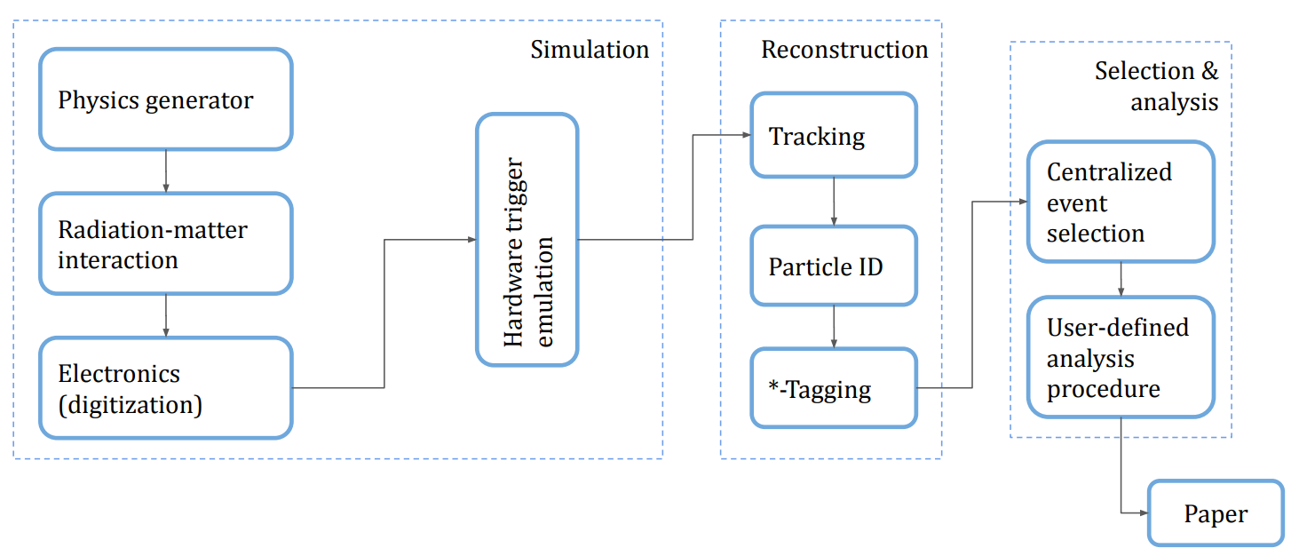
Figure 1: Flowchart of the Detailed Simulation processing

Detailed Simulation provides description based on the physical model of the detector response to the incident particle. As for most HEP experiments, the first step in the simulation of the LHCb experiment [6] is to simulate the proton-proton collisions with a Monte Carlo generator such as PYTHIA [7], EPOS [8], or BcVegPy [9]. The simulation of the heavy hadrons produced in the collision is obtained running EvtGen [10]. The particles produced in primary collisions and in subsequent decays are then propagated through the detector and the energy deposited for radiation-matter interaction is computed with GEANT4 [11]. The energy deposits (or hits) are then digitized [12] and the hardware trigger is emulated [13, 14] in order to provide to the event reconstruction pipeline an input as similar as possible to real data. The reconstruction pipeline is composed of several algorithms dealing with tracking, associating sets of aligned hits to trajectories of charged particles (or tracks), the charged particle identification, assigning to each track a likelihood (or other test statistics) for each mass hypothesis, and neutral object identification mainly intended to identify photons impinging on the calorimeter. A final step in the reconstruction consists of algorithms considering sets of tracks to tag some special property of the event. For example flavour tagging is a technique based on the statistical study of the particles produced in combination with a $b\bar{b}$ quark pair developed to discriminate hadrons produced as $B^{0}$ or $\bar{B}^{0}$ and study flavour oscillations [15, 16, 17, 18].

The reconstructed events are then processed with a centralised selection framework splitting the events in streams depending on the area of the LHCb physics programme. The streams are finally processed by the LHCb members individually to perform statistical analyses on sets of events and draw conclusions on the underlying physics model.

The procedure to obtain Detailed Simulation samples is depicted as a flowchart in Figure 1.

2 Models for the energy depositions in the calorimeters

The most common application of Machine Learning to Simulation is predicting the energy deposits of particles in the electromagnetic calorimeter. Indeed, the detailed simulation of the electromagnetic and hadronic showers in the calorimeters is computational espensive, accounting for more than half of the total CPU demand from the LHC experiments [3, 19]. Intense research activity to speed-up the calorimeter simulation is attested by the many publications on the subject from the ATLAS [20, 21] and CMS [22, 23, 24] Collaborations, but also in the context of the effort towards GeantV [25, 26]. A software package dedicated to the parametric simulation of the calorimeters of ATLAS, CMS and experiments at future colliders is also being developed under the name of Delphes [27].

Both traditional parametrization techniques and methods based on Machine Learning have been explored. When machine learning is employed, it often relies on Deep Convolutional Generative Adversarial Neural Networks (DCGANs) [28] to predict the energy deposited in each active volume (voxel) by taking into account the correlation between adjacent regions. For example, the model developed for the LHCb experiment solutions based on conditional DCGANs [29] and a combination of conditional DCGANs and Variational Autoencoders (VAEs) [30]. In both models the idea is to take as an input the parameters of each particle (either a charged one or a photon) such as its momentum and slopes, and translate them to a randomly generated image of the shower in the electromagnetic calorimeter. The procedure can then be repeated for each track in the event to reconstruct the overall response of the calorimeter.

These methods provide an output which is intended to be processed with the whole reconstruction pipeline. The resulting simulated samples contain all the features exactly as the detailed simulation, including, for example, the tagging information based on collective features. On the other hand, achieving good representation of the reconstructed quantities is challenging because the reconstruction algorithms are not known to the training algorithms, and therefore the reproduction of reconstructed quantities can be optimised only indirectly.

3 Models for the reconstructed quantities

To achieve a further speed-up of the Simulation improving the quality of the reconstructed quantities, Musella and Pandolfi proposed to use GANs to simulate directly the variables obtained from the reconstruction pipeline [31]. This approach allows for a faster and more accurate simulation with respect to the simulation of the energy deposits, but the multi-particle effects on the reconstruction becomes more difficult to take into account because the reconstruction algorithms are parametrise themselves. As a consequence, the high-level physics quantities obtained through the tagging part of the reconstruction pipeline represent an additional challenge in this so called ultra-fast simulation.

Nonetheless, the method had success enabling fast simulation of detectors beyond calorimeters, providing for example the output of the LHCb RICH detectors [32] and muon system [33]. In both cases, a conditional GAN has been trained to reproduce the PID-related observables (or, more technically, the logarithmic likelihood ratio between the muon, kaon, or proton hypothesis and the pion hypothesis). The reconstruction algorithm used to obtain these quantities is rather complex, involving a event-wise modelling of the energy deposits in the calorimeter under various combinations for the mass hypotheses [34], but the effect of inter-particle correlations on the likelihoods, can be effectively modelled by including the detector occupancy among the GAN conditions together with track momentum and pseudorapidity.

4 Training on simulated or real data

The most common procedure to train Generative Models to parametrise the detector response is to generate samples through the Detailed Simulation pipeline and then train the model to associate generator-level variables to reconstructed quantities. This simple technique, however, is intrinsically limited to the quality of the Detailed Simulation or, in other words, a fast simulation obtained training on detailed simulation will be at most as accurate as detailed simulation.

As an interesting alternative, the Generative Models can be trained on real data if following two conditions are satisfied.

• The acquired dataset is unbiased. The training data should be selected without applying selection criteria that, directly or indirectly, modify the distributions of the reconstructed quantities beyond the effect taken into account by the conditions passed as inputs to the Generative Model (such as the kinematics or the detector occupancy). For example, a very common bias is introduced by trigger algorithms designed to select muons. A training sample obtained without excluding candidates selected by these lines will result into Generative Models overestimating the probability of misidentification of hadrons as muons, because the training sample was enriched of hadrons with a detector response more similar to that of a muon than the average hadron. In LHCb this is avoided providing dedicated trigger lines and a dedicated data processing scheme for the calibration data used to train the Generative Models for the ultra-fast simulation [35].

• The generative model supports background subtraction. Calibration samples are usually as abundant and pure as possible, but in order to avoid selection bias, the selections are often loose and some background contribution is expected. For all the models with a loss function derived more or less directly from the maximum likelihood principle, it was demonstrated that weighting the events with properly-computed weights the effect of the background component on the trained network is null [36, 37]. These background-subtracting weights, sometimes called ${}_{s}\mathcal{W}$eights in the context of High Energy Physics, are computed taking into account the models for the signal and the background components in a discriminant variable (e.g. the invariant mass of the combination of reconstructed particles) assumed to be independent of all the other (target) variables involved in the background subtraction [38].

It is worth noticing that an ultra-fast simulation trained on real data is subject to systematic errors in the description of the detector response which are completely independent of the detailed simulation. Detailed and ultra-fast simulation can then cross-check each other, while providing a measure of the simulation accuracy depending on the specific phase space relevant to each analysis.

5 Automatic hyperparameter optimisation for generative models

The training of GANs is well known within the Machine Learning community to be a difficult task [39]. Reaching the Nash equilibrium between the Generator and the Discrminator requires careful tuning of the hyperparameters, such as the learning rate or the network structure. Unfortunately, the absolute value of the loss function used to train adversarial models is not meaningful: a discriminator that finds more difficult to separate real and fake candidates may mean that the generator is better (and so is the accuracy of the generated sample) or that the disciminator is worse (and so is the accuracy of the generated sample).

In order to be able to use Bayesian hyperparameter optimisation frameworks, such as optuna [40] or scikit-optimize [41], LHCb adopted a goodness-of-fit method based on the ability of a BDT classifier to distinguish training and generated data entries [42, 43]. The BDT classifier is a third player, independent of the adversarial training procedure, and is based on a different classification method with different underlying hypotheses. To provide an estimate of the uncertainty on quality metric obtained from the BDT, the same algorithm is trained several times on the same sample with different random seed. The average and its uncertainty are used as guidance for optimising the hyperparameters using a distributed version of optuna, named OptunAPI [44]. With this strategy, it is possible to automate the training of GANs on multiple GPU nodes making the production of a different model per datataking period accessible.

6 Deployment in the software stacks of the experiments

The training and the validation of the generative models relies on Python frameworks such as scikit-learn [45] for the pre- and post-processing stages and either tensorflow [46] or PyTorch [47] for the description of the neural network model.

The pipeline built in Python must then be deployed in the software stack of the experiments, which is most often written in C++ and released few times a year. Both $\mathrm{TenorFlow}$ and PyTorch provide C/C++ APIs to deploy neural network models, however the build system of these large packages often conflicts with the build system of the experiment’s software. The same applies for the multi-thread schedulers, designed to meet the high-throughput requirements of LHC experiments on one side and to speed-up the evaluation of the networks on the other.

In the context of the CMS and LHCb collaborations, $\mathrm{TenorFlow}$ has been succesfully integrated within the experiment software providing evaluations of arbitrarily complicated networks with short latency. A limitation derived from this approach is that all the networks within the experiment software must share the same version of $\mathrm{TenorFlow}$, which makes the maintenance effort rather significant. An intestersting alternative is to provide an inference service external to the experiment software, possibly running on the same machine and interfaced to the data processing software framework via REST APIs [48]. This approach effectively decouples production code and the internal architecture of the server which may be based on whatever framework with whatever thread scheduler and hardware acceleration as long as it is consistent with the REST interface. Several servers can run concurrently to rely on multiple frameworks or framework versions. Due to the large latency, however, this technique is more suitable to process large events with thousands of tracks than to produce ultra-fast simulation, where the time spent per event is of the same order as the REST API latency.

To reduce the latency as much as possible, the ATLAS Collaboration has been developing LWTNN [49], a C++-compiled generic interface for Deep Neural Networks. LWTNN is composed of an engine compiled together with the experiment software and released twice a year, and reads configuration files describing the network architecture and its weights, to reconstruct the model at runtime. To make the evaluation even faster, LHCb has been developing RNNGenerator to produce C++ code for the Neural Network and compile it together with the experiment’s software without any dependence on external frameworks. On the same line, $\mathtt{scikin}$ is a package designed to convert scikit-learn models in C and distribute them as optimised single-thread shared objects. More recently, support to simple Keras [50] feed-forward models was added. Hence, $\mathtt{scikin}$ is much more limited than LWTNN and RNNGenertor in terms of supported architectures, but eliminates almost any overhead and enables the distribution of models, including architecture and weights, as data objects.

The ultra-fast simulation framework of the LHCb Collaboration was originally designed to rely on GaudiTensorFlow, but an implementation based on $\mathtt{scikin}$ was found significantly faster. GaudiTensorFlow is now being phased out and the ultra-fast simulation migrated to $\mathtt{scikin}$.

7 Validation

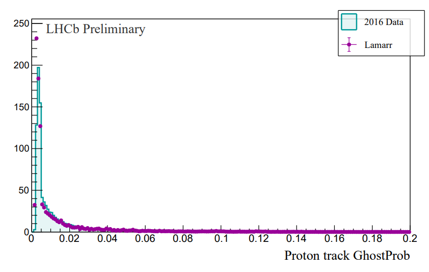
Figure 2: Comparison of the tracking-related variables for protons obtained from tagged $\Lambda_{c}^{+}\to pK^{-}\pi^{+}$ decays in calibration data and through the whole ultra-fast simulation pipeline as implemented in Lamarr. Figure reproduced from Ref. [51].

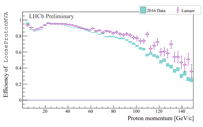
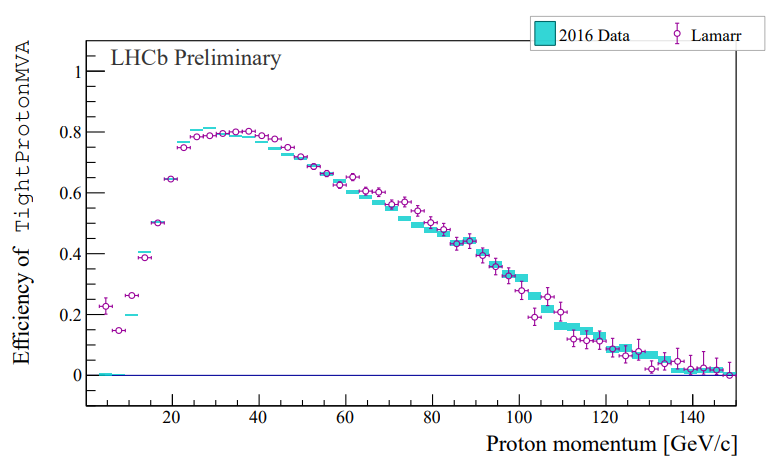
Figure 3: Comparison of the efficiency of two PID requirements with different thresholds as obtained from tagged $\Lambda_{c}^{+}\to pK^{-}\pi^{+}$ decays in calibration data from Lamarr. Figure reproduced from Ref. [51].

The fast-simulation validation campaign is performed comparing data from a calibration sample with the results from Lamarr, the ultra-fast simulation package under development within LHCb. To validate the generalisation properties of the models, different decay models are chosen for the training and the validation of the simulation pipeline. For example, the proton identification is trained using tagged protons from $\Lambda^{0}\to p\pi^{-}$ decays while the validation relies on tagged protons from $\Lambda_{c}^{+}\to pK^{-}\pi^{+}$ decays with the charm hadron produced in the semileptonic decay $\Lambda_{b}^{0}\to\Lambda_{c}^{+}\mu^{-}X$.

Figure 3 reports the comparison between the calibration data and the simulation for the response of a neural network classifier trained to identify ghost tracks and for the logarithm of the impact-parameter $\chi^{2}$, measuring the consistency of the proton track with the primary vertex. The former is a variable directly obtained as an output of a Generative Model, while the latter is computed from the simulated properties of the track and primary vertex, and their (simulated) uncertainties.

Figure 3 shows instead the selection efficiency of a criterion based on the response of classifier trained to distinguish the particle mass combining the response of the whole LHCb Particle Identification apparatus: two RICH detectors, four Muon stations and the electromagnetic calorimeter. In this case of the simulation, the response of the classifier is obtained directly as an output of the generative model. The selection efficiency for two different thresholds are shown as a function of the proton momentum, demonstrating the capability of the Generative Model to properly model the dependence of the detector response on the kinematics of the impinging particle. Similar plots are produced to check good representation of the dependence on the detector occupancy and other conditions. For a deeper discussion of these and additional comparison plots, see Ref. [51].

8 Conclusion

The simulation of the LHCb experiment is an expensive tasks posing severe pressure on the pledged computing resources. Several solutions to speed-up the simulation are being explored, among those Machine-Learning Generative Models are extremely promising. Solutions have been proposed to model both the energy depositions in the calorimeters and the analysis-level quantities features, presenting complementary advantages.

The techniques used to train the model on calibration data enables to go beyond an approximation of the full simulation, obtaining an ultra-fast simulation potentially competitive with the full simulation and providing useful cross-checks.

Both the training and the deployment of Generative Models are active research subjects to keep improving the quality of the simulated features. I discussed as an example the Bayesian hyperparameter optimisation based on OptunAPI, and several deployment strategies with different balance between performance and support to neural network models.

Lamarr, the ultra-fast simulation framework under development in LHCb, combines several traditional parametrisations and Generative Models to produce simulated output as similar as possible to reconstructed data. The comparison of the simulated quantities with calibration samples not used for the training confirms good generalisation properties.

Upcoming releases of Lamarr will improve the quality of the simulation and extend the reach of the simulation by adding several reconstructed quantities, providing a powerful tool within the wide Simulation palette of the LHCb experiment.

References

- [1] LHCb collaboration, The LHCb Detector at the LHC, JINST 3 (2008) S08005.
- [2] LHCb Collaboration collaboration, LHCb Detector Performance, Int. J. Mod. Phys. A 30 (2015) 1530022 [1412.6352].
- [3] T. Boccali, Computing models in high energy physics, Rev. Phys. 4 (2019) 100034.
- [4] LHCb collaboration, “LHCb CPU Usage Forecast.” LHCb-FIGURE-2019-18, 2019.
- [5] D. Müller, M. Clemencic, G. Corti and M. Gersabeck, ReDecay: A novel approach to speed up the simulation at LHCb, Eur. Phys. J. C 78 (2018) 1009 [1810.10362].
- [6] LHCb collaboration, Handling of the generation of primary events in Gauss, the LHCb simulation framework, J. Phys. Conf. Ser. 331 (2011) 032047.
- [7] T. Sjostrand, S. Mrenna and P.Z. Skands, A Brief Introduction to PYTHIA 8.1, Comput. Phys. Commun. 178 (2008) 852 [0710.3820].
- [8] T. Pierog, I. Karpenko, J.M. Katzy, E. Yatsenko and K. Werner, EPOS LHC: Test of collective hadronization with data measured at the CERN Large Hadron Collider, Phys. Rev. C 92 (2015) 034906 [1306.0121].
- [9] C.-H. Chang, J.-X. Wang and X.-G. Wu, BCVEGPY2.0: A Upgrade version of the generator BCVEGPY with an addendum about hadroproduction of the P-wave B(c) states, Comput. Phys. Commun. 174 (2006) 241 [hep-ph/0504017].
- [10] D.J. Lange, The EvtGen particle decay simulation package, Nucl. Instrum. Meth. A 462 (2001) 152.
- [11] GEANT4 collaboration, GEANT4–a simulation toolkit, Nucl. Instrum. Meth. A 506 (2003) 250.
- [12] G. Corti, M. Cattaneo, P. Charpentier, M. Frank, P. Koppenburg, P. Mato et al., Software for the LHCb experiment, IEEE Trans. Nucl. Sci. 53 (2006) 1323.
- [13] R. Aaij et al., The LHCb Trigger and its Performance in 2011, JINST 8 (2013) P04022 [1211.3055].
- [14] LHCb collaboration, Design and performance of the LHCb trigger and full real-time reconstruction in Run 2 of the LHC, JINST 14 (2019) P04013 [1812.10790].
- [15] LHCb collaboration, New algorithms for identifying the flavour of mesons using pions and protons, Eur. Phys. J. C 77 (2017) 238 [1610.06019].
- [16] LHCb collaboration, A new algorithm for identifying the flavour of mesons at LHCb, JINST 11 (2016) P05010 [1602.07252].
- [17] LHCb collaboration, flavour tagging using charm decays at the LHCb experiment, JINST 10 (2015) P10005 [1507.07892].
- [18] LHCb collaboration, Opposite-side flavour tagging of B mesons at the LHCb experiment, Eur. Phys. J. C 72 (2012) 2022 [1202.4979].
- [19] C. Bozzi, LHCb Computing Resources: update of 2021 requests, LHCb-PUB-2020-001, Tech. Rep. (2020).
- [20] ATLAS collaboration, AtlFast3: the next generation of fast simulation in ATLAS, 2109.02551.
- [21] C. Krause and D. Shih, CaloFlow: Fast and Accurate Generation of Calorimeter Showers with Normalizing Flows, 2106.05285.
- [22] M. Paganini, L. de Oliveira and B. Nachman, CaloGAN : Simulating 3D high energy particle showers in multilayer electromagnetic calorimeters with generative adversarial networks, Phys. Rev. D 97 (2018) 014021 [1712.10321].
- [23] R. Rahmat, R. Kroeger and A. Giammanco, The fast simulation of the CMS experiment, J. Phys. Conf. Ser. 396 (2012) 062016.
- [24] CMS collaboration, The fast simulation of the CMS detector at LHC, J. Phys. Conf. Ser. 331 (2011) 032049.
- [25] G. Amadio et al., GeantV Alpha Release, J. Phys. Conf. Ser. 1085 (2018) 032037.
- [26] G.R. Khattak, S. Vallecorsa, F. Carminati and G.M. Khan, Fast Simulation of a High Granularity Calorimeter by Generative Adversarial Networks, 2109.07388.
- [27] DELPHES 3 collaboration, DELPHES 3, A modular framework for fast simulation of a generic collider experiment, JHEP 02 (2014) 057 [1307.6346].
- [28] A. Radford, L. Metz and S. Chintala, Unsupervised representation learning with deep convolutional generative adversarial networks, 1511.06434.
- [29] V. Chekalina, E. Orlova, F. Ratnikov, D. Ulyanov, A. Ustyuzhanin and E. Zakharov, Generative Models for Fast Calorimeter Simulation: the LHCb case, EPJ Web Conf. 214 (2019) 02034 [1812.01319].
- [30] F. Sergeev, N. Jain, I. Knunyants, G. Kostenkov and E. Trofimova, Fast simulation of the LHCb electromagnetic calorimeter response using VAEs and GANs, J. Phys. Conf. Ser. 1740 (2021) 012028.
- [31] P. Musella and F. Pandolfi, Fast and Accurate Simulation of Particle Detectors Using Generative Adversarial Networks, Comput. Softw. Big Sci. 2 (2018) 8 [1805.00850].
- [32] LHCb collaboration, Fast Data-Driven Simulation of Cherenkov Detectors Using Generative Adversarial Networks, J. Phys. Conf. Ser. 1525 (2020) 012097 [1905.11825].
- [33] G. Sassoli, Generative Adversarial Networks for the Ultra-Fast Simulation of the Muon Detector of the LHCb experiment at CERN, Thesis discussed in July 2019, University of Florence .
- [34] LHCb RICH Group collaboration, Performance of the LHCb RICH detector at the LHC, Eur. Phys. J. C 73 (2013) 2431 [1211.6759].
- [35] R. Aaij et al., Selection and processing of calibration samples to measure the particle identification performance of the LHCb experiment in Run 2, EPJ Tech. Instrum. 6 (2019) 1 [1803.00824].
- [36] Y. Xie, sFit: a method for background subtraction in maximum likelihood fit, 0905.0724.
- [37] M. Borisyak and N. Kazeev, Machine Learning on data with sPlot background subtraction, JINST 14 (2019) P08020 [1905.11719].
- [38] M. Pivk and F.R. Le Diberder, SPlot: A Statistical tool to unfold data distributions, Nucl. Instrum. Meth. A 555 (2005) 356 [physics/0402083].
- [39] I.J. Goodfellow, J. Pouget-Abadie, M. Mirza, B. Xu, D. Warde-Farley, S. Ozair et al., Generative adversarial nets, in Proceedings of the 27th International Conference on Neural Information Processing Systems - Volume 2, NIPS’14, (Cambridge, MA, USA), p. 2672–2680, MIT Press, 2014.
- [40] T. Akiba, S. Sano, T. Yanase, T. Ohta and M. Koyama, Optuna: A next-generation hyperparameter optimization framework, 2019.
- [41] T. Head, M. Kumar, H. Nahrstaedt, G. Louppe and I. Shcherbatyi, scikit-optimize/scikit-optimize, Sept., 2020. 10.5281/zenodo.4014775.
- [42] M. Williams, How good are your fits? Unbinned multivariate goodness-of-fit tests in high energy physics, JINST 5 (2010) P09004 [1006.3019].
- [43] C. Weisser and M. Williams, Machine learning and multivariate goodness of fit, 1612.07186.
- [44] M. Barbetti, mbarbetti/optunapi, Zenodo (2021) 5538989.
- [45] F. Pedregosa, G. Varoquaux, A. Gramfort, V. Michel, B. Thirion, O. Grisel et al., Scikit-learn: Machine learning in Python, Journal of Machine Learning Research 12 (2011) 2825.
- [46] TensorFlow Developers, Tensorflow, Zenodo (2021) 5189249.
- [47] A. Paszke, S. Gross, F. Massa, A. Lerer, J. Bradbury, G. Chanan et al., Pytorch: An imperative style, high-performance deep learning library, Advances in Neural Information Processing Systems (2019) 8024.
- [48] V. Kuznetsov, L. Giommi and D. Bonacorsi, MLaaS4HEP: Machine Learning as a Service for HEP, Comput. Softw. Big Sci. 5 (2021) 17 [2007.14781].
- [49] D.H. Guest, J.W. Smith, M. Paganini, M. Kagan, M. Lanfermann, A. Krasznahorkay et al., lwtnn/lwtnn: Version 2.12.1, Zenodo (2021) 5082190.
- [50] F. Chollet et al., “Keras.” https://keras.io, 2015.
- [51] LHCb collaboration, “Performance of the Lamarr Prototype: the ultra-fast simulation option integrated in the LHCb simulation framework.” LHCb-FIGURE-2019-17, 2019.