Andrew David Pearce and Armin Hatefi

Department of Mathematics and Statistics, Memorial University of Newfoundland, St. John’s, NL, Canada.

Ranked set sampling (RSS) is used as a powerful data collection technique for situations where measuring the study variable requires a costly and/or tedious process while the sampling units can be ranked easily (e.g., osteoporosis research). In this paper, we develop ridge and Liu-type shrinkage estimators under RSS data from multiple observers to handle the collinearity problem in estimating coefficients of linear regression, stochastic restricted regression and logistic regression. Through extensive numerical studies, we show that shrinkage methods with the multi-observer RSS result in more efficient coefficient estimates. The developed methods are finally applied to bone mineral data for analysis of bone disorder status of women aged 50 and older.

Keywords: Ranked set sampling, Multiple observer, collinearity, Ridge estimator, Stochastic restricted regression, Logistic regression.

1 Introduction

In many medical surveys (e.g., osteoporosis research), measuring the response variable (e.g., diagnosis osteoporosis status) requires a costly and tedious process. Despite this challenge, practitioners typically have access to many easily attainable concomitants (e.g., demographic and laboratory characteristics). In these situations, the research question is how to incorporate these easy-to-measure characteristics into data collection and obtain more representative samples from the population.

As a bone metabolic disorder, osteoporosis happens when the density of bone structure of the body reduces significantly. This significant reduction leads to various major health problems, including susceptibility to skeletal fragility and osteoporotic fractures in the hip and femoral area (Black et al., 1992, Cummings et al., 1995). About 33% of women and 20% of men experience an osteoporotic fracture in the age group of 50 and older (Melton III et al., 1998). More than 50% of individuals who experienced an osteoporotic hip fracture will no longer be able to live independently and about 28% of them will die within one year from complications of the fractured bone (Bliuc et al., 2009, Neuburger et al., 2015). As the aged population increases in many countries, one should anticipate a rise in the prevalence of osteoporosis-related health problems.

The expert panel of WHO introduces the Bone Mineral Density (BMD) as the most reliable factor for bone disorder analysis and diagnosis. Despite this reliability, measuring BMD is costly and tedious. BMD measurements are taken from dual X-ray absorptiometry (DXA) imaging. Once images are taken, medical experts are needed for manual segmentation of images and extracting necessary measurements. While measuring BMD is difficult, clinicians typically have access to easily attainable characteristics about patients such as weight, BMI, age and BMD scores from earlier surveys. We believe ranked set sampling, as a cost-effective technique, can be used to incorporate these characteristics into data collection and results in more efficient estimates for the parameters of the osteoporosis population.

To construct an RSS (i.e., ranked set sampling/sample) from the osteoporosis population, first $H^{2}$ patients are identified and allocated to $H$ sets of size $H$. Patients are then ranked (without measuring their BMD) using an inexpensive characteristic (e.g., age). We select the individual with rank $r$ from the $r$-th set ($r=1,\ldots,H$) and measure her BMD score. This results in an RSS of size $H$. The cycle is then repeated $n$ times to find a balanced RSS sample of size $N=nH$. RSS has found applications in a wide variety of fields such as breast cancer (Hatefi and Jafari Jozani, 2017, Zamanzade and Wang, 2018), osteoporosis (Nahhas et al., 2002), education (Wang et al., 2016), environments (Amiri et al., 2014, Ozturk, 2014, Frey, 2012), fishery (Hatefi et al., 2015), trauma (Helu et al., 2011) to name a few.

Collinearity is one of the most common issues in linear regression and logistic regression. In the presence of collinearity, the least squares estimates become unreliable and lead us to misleading results. Despite a rich literature of RSS data for linear regression and logistics regression(Lynne Stokes, 1977, Muttlak, 1995, Zamanzade and Wang, 2018, Chen et al., 2005, Hatefi and Alvandi, 2020, Alvandi and Hatefi, 2021), there are very few works investigated the RSS for shrinkage estimates to cope with the collinearity issue. Although Ebegil et al. (2021) recently proposed ridge and Liu-type estimators with median RSS for the collinearity, the proposed shrinkage estimators are only developed for the linear regression model (i.e., continuous response). In addition, the developed RSS estimators can only use a single characteristic for ranking involved in RSS. Plus, the methods are not capable of using the ties information in RSS data.

Despite the importance of logistic regression in medical studies, to our best knowledge, there is no research in literature investigated the use of RSS data for shrinkage methods to deal with the collinearity issue in logistic regression and stochastic restricted regression models. While Zamanzade and Wang (2018), Chen et al. (2005), Hatefi and Alvandi (2020), Alvandi and Hatefi (2021) used RSS data for analysis of logistic regression and binary data, the research question here differs from them. In this manuscript, we shall employ RSS data to develop shrinkage estimators for the coefficients of the logistic regression. Unlike Chen et al. (2005), the estimation methods here do not require training data. While Zamanzade and Wang (2018), Chen et al. (2005), Alvandi and Hatefi (2021) focus on logistic regression where the population proportion is fixed, here we treat the response prevalence $\pi({\bf x})$ in a general form (i.e., as the generalized linear function of predictors) so that it changes from one individual to another and is of course subject to collinearity issue. In this manuscript, we use multi-observer RSS of Alvandi and Hatefi (2021) that inherits the tie flexibility of Frey (2012) and multiple observers of (Ozturk, 2013) in data collection. We then develop ridge and Liu type estimators under multi-observer RSS to overcome the collinearity issue in linear regression, stochastic restricted regression and logistic regression. The developed methods are finally applied to bone mineral data for analysis of bone disorder status of women aged 50 and older.

This manuscript is organized as follows. Section 2 describes the construction of RSS data from multiple observers. The development of shrinkage methods with SRS and RSS data are discussed in Sections 3 and 4. The estimation methods are evaluated through various simulation studies and real data examples in Sections 5 and 6. Summary and concluding remarks are finally presented in Section 7.

2 Multi-observer RSS

Frey (2012) introduced an RSS method that is able to incorporate as many tied units as desired into data collection. Despite this flexibility, this RSS scheme can only use a single observer for ranking in RSS. Alvandi and Hatefi (2021) proposed an RSS scheme that simultaneously enjoys the tie information of (Frey, 2012) and multiple observers of (Ozturk, 2013). In this manuscript, we investigate the properties of multi-observer RSS data of (Alvandi and Hatefi, 2021) to deal with the collinearity issue.

Let $({\bf X},{\bf y})$ denote a multivariate random variable where ${\bf y}$ and ${\bf X}=({\bf x}_{1},\ldots,{\bf x}_{p})$ denote the response vector and the design matrix with $p$ predictors, respectively. Suppose ${\bf R}=(R_{1},\ldots,R_{K})$ is the vector of $K$ easy-to-measure external concomitant variables which are used for ranking purposes in RSS.

In this manuscript, we focus on balanced multi-observer RSS (MRS) data. Let $H$ and $n$ denote set and cycle sizes of the scheme, respectively. To collect MRS data of size $N=nH$, similar to the standard RSS (described in Section 1), we plan to measure the $r$-th judgemental order statistic $Y_{[r]j}$ from the $r$-th set in the $j$-th cycle. Let ${\bf U}^{[r]}_{j}=(u^{[r]}_{1,j},\ldots,u^{[r]}_{H,j})$ represent the $H$ units in the $r$-th set. We rank the units with respect to their corresponding concomitant variables ${\bf R}^{[r]}_{k,j}=({R}^{[r]}_{1,k,j},\ldots,{R}^{[r]}_{H,k,j})$ for $k=1,\ldots,K$. Suppose ${\bf W}^{[r]}_{k,j}$ denotes the weight matrix (of size $H\times H$) that records the ranks and ties information assigned by observer ${\bf R}^{[r]}_{k,j}$. Frey (2012) introduced the Discrete Perceived size (DPS) model to implement the tie in RSS. The DPS model gives a tied rank to units $u^{[r]}_{l_{1},j}$ and $u^{[r]}_{l_{2},j}$ if $[u^{[r]}_{l_{1},j}/c]=[u^{[r]}_{l_{2},j}/c]$, where $[\cdot]$ indicates the floor function and $c$ is a user-chosen parameter. If unit $u^{[r]}_{l_{1},j}$ receives rank $l_{2}$ by observer ${\bf R}^{[r]}_{k,j}$, the $(l_{1},l_{2})$ entry of ${\bf W}^{[r]}_{k,j}$ becomes one; otherwise the entry will be zero. Once we recorded weight matrices ${\bf W}^{[r]}_{k,j}$ for $k=1,\ldots,K$, the ranking information is combined by

$${\bar{\bf W}}^{[r]}_{j}=\sum_{k=1}^{K}\eta_{k}{\bf W}^{[r]}_{k,j},~{}~{}~{}~{}~{}~{}~{}\eta_{k}=\frac{|\rho_{k}|}{\sum_{k^{\prime}=1}^{K}|\rho_{k^{\prime}}|}$$

where $\rho_{k}$ denotes the correlation between $R_{k}$ and ${\bf y}$. The unit with the highest weight in the $r$-th column of ${\bar{\bf W}}^{[r]}_{j}$ is then selected and measured with response $Y_{[r]j}$ and $p$ predictors ${\bf X}_{[r]j}=(x_{1[r]j},\ldots,x_{p[r]j})$. In a similar fashion, we measure other MRS statistics. Eventually, the MRS data (of size $N=nH$) is given by $\{(Y_{[r]j},{\bf X}_{[r]j},{\bar{w}}^{[r]}_{j});r=1,\ldots,H;j=1,\ldots,n\}$.

In the multi-observer RSS scheme of (Alvandi and Hatefi, 2021), one can measure different order statistics from different sets. While this proposal gives us information from all aspects of the population, measuring only medians from all sets may be more beneficial when the population is symmetric. To this end, here we generalize the multi-observer RSS (MRS) of (Alvandi and Hatefi, 2021) to median multi-observer RSS (MMR) scheme where we always measure medians from ${\bf U}^{[r]}_{j}$ sets for $r=1,\ldots,H$. Accordingly, the MMR data of size $nH$ is given by $\{(Y_{[l]j},{\bf X}_{[l]j},{\bar{w}}^{[l]}_{j});j=1,\ldots,nH\}$ where $l=(H+1)/2$ when $H$ is odd and when $H$ is even, we use $H/2$ for the first $N/2$ observations and $H/2+1$ for the other half. For more details about the milt-observer RSS and median RSS scheme, see (Alvandi and Hatefi, 2021, Samawi and Al-Sagheer, 2001, Ozturk, 2013) and references therein.

3 Estimation Methods with SRS

Multiple linear regression model has found applications in many fields. Suppose the model is given by

$${\bf y}={\bf X}{\bf\beta}+{\bf\epsilon},$$ (1)

where $\bf\beta$ represents the unknown coefficients of the model, ${\bf y}$ is $(N\times 1)$ vector of responses and ${\bf X}$ represents non-random $(N\times p)$ design matrix of $p$ explanatory variables $({\bf x}_{1},\ldots,{\bf x}_{p})$ with $\text{rank}({\bf X})=p<N$. Assume ${\bf\epsilon}\sim N({\bf 0},\sigma^{2}\mathbb{I}_{N})$, with $\mathbb{E}({\bf\epsilon})={\bf 0}$ and $\text{Var}({\bf\epsilon})=\sigma^{2}\mathbb{I}_{N}$ where $\sigma^{2}$ is the common variance of error and $\mathbb{I}_{N}$ is $N$ dimensional identity matrix. Let ${\bf S}={\bf X}^{\top}{\bf X}$ henceforth. The regression model (1) can also be viewed in a canonical form. Using an orthogonal matrix $U$, one can diagonalize ${\bf S}$ by $U^{\top}{\bf S}U=\Lambda$ where $\Lambda=\text{diag}(\lambda_{1},\ldots,\lambda_{p})$ with $\lambda_{1}>\ldots>\lambda_{p}$ are the eigenvalues of ${\bf S}$. In the canonical form, the regression model (1) becomes ${\bf y}={\bf Z}{\bf\gamma}+{\bf\epsilon},$ where ${\bf Z}={\bf X}^{\top}U$ and ${\bf\gamma}=U^{\top}{\bf\beta}$.

Least square method is the most common method to estimate the coefficients of the regression model (1). The Least Squares (LS) estimator of ${\bf\beta}$ is then given by

$${\widehat{\bf\beta}}_{LS}={\bf S}^{-1}{\bf X}^{\top}{\bf y}.$$ (2)

One big challenge of ${\widehat{\bf\beta}}_{LS}$ occurs in the presence of collinearity where the explanatory variables are linearly dependent. The Ridge method is considered as a solution to the problem. The ridge estimator ${\widehat{\bf\beta}}_{R}$ is given by

$${\widehat{\bf\beta}}_{R}=({\bf S}+k\mathbb{I})^{-1}{\bf X}^{\top}{\bf y},$$ (3)

where $k$ represents the ridge parameter. When the collinearity arises, the matrix ${\bf S}$ is then considered ill-conditioned; hence ${\bf S}^{-1}$ becomes practically singular. The ridge method suggests to add $k$ to the diagonal elements of the ill-conditioned matrix ${\bf S}$ at the price of introducing a bias in the estimation procedure. When the collinearity is more sever, the ridge parameter alone may not be enough to overcome the ill-conditioned matrix. Kejian (2003) proposes the Liu-type method as follows

$${\widehat{\bf\beta}}_{LT}=({\bf S}+k\mathbb{I})^{-1}({\bf X}^{\top}{\bf y}+d{\widehat{\bf\beta}}_{R}),$$ (4)

where $k>0$, $d\in\mathbb{R}$ and ${\widehat{\bf\beta}}_{R}$ is given by (3).

3.1 Stochastic Restricted Estimators

In many situations, in addition to the regression model (1), one has prior information about the coefficients of the model in a form of a set of $j$ independent stochastic restrictions as

$${\bf r}={\bf R}{\bf\beta}+{\bf e},$$ (5)

where ${\bf r}$ is a $(j\times 1)$ vector known responses, ${\bf R}$ is a $(j\times p)$ known matrix and ${\bf e}$ is a random vector with $\mathbb{E}({\bf e})={\bf 0}$, $\text{Var}({\bf e})=\sigma^{2}{\bf\Omega}$ where ${\bf\Omega}$ is assumed to be a known semi-positive matrix. Assume that ${\bf e}$ and ${\bf\epsilon}$ are stochastically independent. For more information about the regression model with stochastic restrictions, see (Yang et al., 2009, Li and Yang, 2010). Using the stochastic restrictions (5), Theil and Goldberger (1961) introduced a weighted mixed estimator ${\widehat{\bf\beta}}_{\text{ME}}$ as

$${\widehat{\bf\beta}}_{\text{ME}}=({\bf S}+v{\bf R}^{\top}{\bf\Omega}^{-1}{\bf R})^{-1}({\bf X}^{\top}{\bf y}+v{\bf R}^{\top}{\bf\Omega}^{-1}{\bf r}),$$ (6)

where $v$ is a non-stochastic scalar weight $0<v\leq 1$. In the presence of collinearity, Hubert and Wijekoon (2006) employed one parameter Liu estimate of (Kejian, 1993) in the context of stochastic restricted regression. Hence, they proposed Mixed Liu estimator of ${\bf\beta}$ as follows

$${\widehat{\bf\beta}}_{\text{MXL}}=({\bf S}+\mathbb{I})^{-1}({\bf S}+d\mathbb{I}){\widehat{\bf\beta}}_{\text{ME}},$$ (7)

where ${\widehat{\bf\beta}}_{\text{ME}}$ is given by (6) and $d\in\mathbb{R}$. Yang and Xu (2009) replaced ${\widehat{\bf\beta}}_{LS}$ with ${\widehat{\bf\beta}}_{LT}$ in mixed estimation method. Accordingly, they proposed an alternative stochastic restricted Liu estimator as follows

$${\widehat{\bf\beta}}_{\text{SRL}}={\widehat{\bf\beta}}_{LT1}+v{\bf S}^{-1}{\bf R}^{\top}({\bf\Omega}+v{\bf R}{\bf S}^{-1}{\bf R}^{\top})^{-1}({\bf r}-{\bf R}{\widehat{\bf\beta}}_{LT1}).$$ (8)

where ${\widehat{\bf\beta}}_{\text{LT1}}$ of (Kejian, 1993) is given by

$${\widehat{\bf\beta}}_{\text{LT1}}=({\bf S}+\mathbb{I})^{-1}({\bf S}+d\mathbb{I}){\widehat{\bf\beta}}_{LS}.$$ (9)

As another method to handle the collinearity, Li and Yang (2010) used the properties of the ridge estimator in the context of stochastic restricted regression and defined mixed ridge estimator as follows

$${\widehat{\bf\beta}}_{\text{MXL}}=(\mathbb{I}+k{\bf S}^{-1})^{-1}{\widehat{\bf\beta}}_{\text{ME}},$$ (10)

where ${\widehat{\bf\beta}}_{\text{ME}}$ is given by (6). Arumairajan et al. (2014) employed ${\widehat{\bf\beta}}_{\text{R}}$ of (3) in mixed estimation method (6) to deal with collinearity. Hence, the stochastic restricted ridge estimator ${\widehat{\bf\beta}}_{\text{SRR}}$ is given by

$${\widehat{\bf\beta}}_{\text{SRR}}={\widehat{\bf\beta}}_{R}+v{\bf S}^{-1}{\bf R}^{\top}({\bf\Omega}+v{\bf R}{\bf S}^{-1}{\bf R}^{\top})^{-1}({\bf r}-{\bf R}{\widehat{\bf\beta}}_{R}).$$ (11)

3.2 Logistic Regression Estimators with SRS

Logistic regression model plays a key role in analysis of binary responses. Let logistic model follow

$$\mathbb{P}(y_{i}=1|{\bf X})=g({\bf x}_{i};{\bf\beta})=1/(1+\exp(-{\bf x}_{i}^{\top}{\bf\beta})),$$ (12)

where $\bf\beta$ represents the coefficients of the model, ${\bf y}$ is vector of binary responses, $g$ as the link function and ${\bf X}$ is non-random $(n\times p)$ design matrix of $p$ explanatory variables $({\bf x}_{1},\ldots,{\bf x}_{p})$ with $\text{rank}({\bf X})=p<N$.

The Maximum likelihood (ML) method is the common method to estimate the coefficients of logistic model (12). The log-likelihood function of ${\bf\beta}$ is given by

$$l({\beta})=\sum_{i=1}^{n}-\log\left(1+\exp(-{\bf x}_{i}^{\top}{\bf\beta})\right)+y_{i}({\bf x}_{i}^{\top}{\bf\beta}).$$ (13)

In the absence of a closed-form maximum of (13), one can find the ML estimate ${\widehat{\bf\beta}_{\text{ML}}}$ using Newton Raphson (NR) method. To do so, given ${\bf\beta}^{(l)}$ the estimate from $l$-th iteration, we iteratively update ${\bf\beta}^{(l+1)}$ as follows

$${\bf\beta}^{(l+1)}={\bf\beta}^{(l)}-{\bf H}^{-1}\left(l({\bf\beta}^{(l)})\right){\nabla}_{\beta}l({\bf\beta}^{(l)}),$$ (14)

where ${\bf H}^{-1}\left(l({\bf\beta}^{(l)})\right)$ and ${\nabla}_{\beta}l({\bf\beta}^{(l)})$ are the Hessian matrix and the gradient evaluated at ${\bf\beta}^{(l)}$, respectively.

The ${\widehat{\bf\beta}_{\text{ML}}}$ is also severely affected when there exists a collinearity problem in the logistic regression. To deal with the collinearity, Schaefer et al. (1984) introduced a ridge estimator as follows

$${\widehat{\bf\beta}}_{\text{R,log}}=({\bf X}^{\top}{\bf V}{\bf X}+k\mathbb{I})^{-1}{\bf X}^{\top}{\bf V}{\bf X}{\widehat{\bf\beta}_{\text{ML}}}.$$ (15)

When collinearity is severe, ${\widehat{\bf\beta}}_{\text{R,log}}$ may not be able to cope with the ill-conditioned matrix. Inan and Erdogan (2013) proposed the Liu-type logistic estimator with $k>0$, $d\in\mathbb{R}$ as follows

$${\widehat{\bf\beta}}_{\text{LT,log}}=({\bf X}^{\top}{\bf V}{\bf X}+k\mathbb{I})^{-1}({\bf X}^{\top}{\bf V}{\bf X}-d\mathbb{I}){\widehat{\bf\beta}_{ML}}.$$ (16)

To obtain the ridge parameter $k$, there are three common choices for $k$ (Schaefer et al., 1984, Inan and Erdogan, 2013). They include $1/{\widehat{\bf\beta}}_{ML}^{\top}{\widehat{\bf\beta}_{ML}},p/{\widehat{\bf\beta}}_{ML}^{\top}{\widehat{\bf\beta}_{ML}},(p+1)/{\widehat{\bf\beta}}_{ML}^{\top}{\widehat{\bf\beta}_{ML}}$ where $p$ denotes the number of predictors in the model. In this manuscript, we select $k$ using ${\widehat{k}}=(p+1)/{\widehat{\bf\beta}}_{ML}^{\top}{\widehat{\bf\beta}_{ML}}$. To determine $d$, Inan and Erdogan (2013) proposed a numerical approach to find the optimal $d$ value which minimizes the mean square errors (MSE) of ${\widehat{\bf\beta}}_{\text{LT,log}}$.

4 Estimation Methods with RSS

In this section, we shall use multi-observer RSS (MRS) to develop shrinkage estimators for the parameters of regression model (1), stochastic restricted model (5) and logistic regression model (12). Although Ebegil et al. (2021) recently develop ridge and Liu-type estimators based on median RSS data for regression model (1), their method is not capable of combining ranking information from multiple sources in data collection. In addition, to our best knowledge, there is no research work investigating the RSS for shrinkage estimation in stochastic restricted regression model and logistic regression in the presence of colinearilty.

We first investigate the estimation of regression model (1) based on MRS data. As described in Section 2, with set size $H$ and cycle size $n$, let ${\bf X}_{\text{MRS}}$ be $(nH\times p)$ design matrix and ${\bf y}_{\text{MRS}}$ be $(nH\times 1)$ response vector based on MRS data when we ignore the weights. Let ${\bf S}_{\text{MRS}}={\bf X}_{\text{MRS}}^{\top}{\bf X}_{\text{MRS}}$ henceforth. Based on MRS data, the least square estimator of ${\bf\beta}$ is given by

$${\widehat{\bf\beta}}_{\text{LS,MRS}}={\bf S}_{\text{MRS}}^{-1}{\bf X}_{\text{MRS}}^{\top}{\bf y}_{\text{MRS}}.$$ (17)

Lemma 1.

$\mathbb{E}({\widehat{\bf\beta}}_{\text{LS,MRS}})={\bf\beta}$ and $\text{Var}({\widehat{\bf\beta}}_{\text{LS,MRS}})=\sigma^{2}{\bf S}_{\text{MRS}}^{-1}.$

While ${\widehat{\bf\beta}}_{\text{LS,MRS}}$ is an unbiased estimator for ${\bf\beta}$, it is severely influenced by collinearity issue. Following (Schaefer et al., 1984, Ebegil et al., 2021), one possible solution is to develop the ridge estimator of ${\bf\beta}$. Hence, the ridge estimator based on MRS data is given by

$${\widehat{\bf\beta}}_{\text{R,MRS}}=({\bf S}_{\text{MRS}}+k\mathbb{I})^{-1}{\bf X}_{\text{MRS}}^{\top}{\bf y}_{\text{MRS}}.$$ (18)

Lemma 2.

The expected value and covariance matrix of ${\widehat{\bf\beta}}_{\text{R,MRS}}$ are given by $\mathbb{E}({\widehat{\bf\beta}}_{\text{R,MRS}})={\bf W}_{\text{MRS}}{\bf\beta}$ and $\text{Var}({\widehat{\bf\beta}}_{\text{R,MRS}})=\sigma^{2}{\bf W}_{\text{MRS}}{\bf S}_{\text{MRS}}^{-1}{\bf W}_{\text{MRS}}^{\top}$ where ${\bf W}_{\text{MRS}}=(\mathbb{I}+k{\bf S}_{\text{MRS}}^{-1})^{-1}$.

Note that ${\widehat{\bf\beta}}_{\text{R,MRS}}$ is obtained by least square solution to the model ${\bf y}_{\text{MRS}}={\bf X}_{\text{MRS}}{\bf\beta}+{\bf\epsilon}$ subject to ${\bf 0}=k^{\frac{1}{2}}{\bf\beta}+\epsilon^{\top}$. As the ridge parameter increases, Lemma 2 shows that the bias of ${\widehat{\bf\beta}}_{\text{R,MMR}}$ increases. For this reason, it is advantageous to choose small $k$ in the ridge estimate. When $k$ is small, $({\bf S}_{\text{MMR}}+k\mathbb{I})$ may still be ill-conditioned. Hence, the Liu-type estimator of ${\bf\beta}$ based on MRS data is given by:

$${\widehat{\bf\beta}}_{\text{LT,MRS}}=({\bf S}_{\text{MRS}}+k\mathbb{I})^{-1}({\bf X}_{\text{MRS}}^{\top}{\bf y}_{\text{MRS}}+d{\widehat{\bf\beta}}_{\text{R,MRS}}),$$ (19)

where $k>0$, $d\in\mathbb{R}$ and ${\widehat{\bf\beta}}_{\text{R,MRS}}$ is given by (18).

Lemma 3.

The expected value and covariance of ${\widehat{\bf\beta}}_{\text{LT,MRS}}$ are given by $\mathbb{E}({\widehat{\bf\beta}}_{\text{LT,MRS}})={\bf A}_{\text{LT,MRS}}{\bf\beta}$ and $\text{Var}({\widehat{\bf\beta}}_{\text{LT,MRS}})=\sigma^{2}{\bf A}_{\text{LT,MRS}}{\bf S}_{\text{MRS}}^{-1}{\bf A}_{\text{LT,MRS}}^{\top}$ where ${\bf A}_{\text{LT,MRS}}=({\bf S}_{\text{MRS}}+k\mathbb{I})^{-1}\left(\mathbb{I}+d({\bf S}_{\text{MRS}}+k\mathbb{I}\right)^{-1}){\bf S}_{\text{MRS}}$.

4.1 Stochastic Restricted Regression with RSS

Here, we employ the MRS data to estimate ${\bf\beta}$ in stochastic restricted regression model (5). We first require the following Lemma (whose proof can be found in Rao and Toutenburg (1995)).

Lemma 4.

Let $A$ and $C$ be nonsingular matrices and $B$ and $D$ be matrices of proper orders. Then $(A+BCD)^{-1}=A^{-1}-A^{-1}B(C^{-1}+CA^{-1}B)DA^{-1}.$

Lemma 5.

Under the assumption of regression model (5) and Lemma 4,

• the weighted mixed estimator from MRS data is given by

  $${\widehat{\bf\beta}}_{\text{ME,MRS}}=({\bf S}_{\text{MRS}}+v{\bf R}^{\top}{\bf\Omega}^{-1}{\bf R})^{-1}({\bf X}_{\text{MRS}}^{\top}{\bf y}_{\text{MRS}}+v{\bf R}^{\top}{\bf\Omega}^{-1}{\bf r}),$$

  where $v$ is a non-stochastic scalar weight $0<v\leq 1$.

• ${\widehat{\bf\beta}}_{\text{ME,MRS}}$ can be written as a function of ${\widehat{\bf\beta}}_{\text{LS,MRS}}$ as

  $${\widehat{\bf\beta}}_{\text{ME,MRS}}={\widehat{\bf\beta}}_{\text{LS,MRS}}+v{\bf S}_{\text{MRS}}^{-1}{\bf R}^{\top}({\bf\Omega}+v{\bf R}{\bf S}_{\text{MRS}}^{-1}{\bf R}^{\top})^{-1}({\bf r}-{\bf R}{\widehat{\bf\beta}}_{\text{LS,MRS}}).$$

The performance of ${\widehat{\bf\beta}}_{\text{ME,MMR}}$, as a function of ${\widehat{\bf\beta}}_{\text{LS,MMR}}$, is severely affected with collinearity. To overcome the problem, the first solution can be to incorporate the method of Hubert and Wijekoon (2006) into ${\widehat{\bf\beta}}_{\text{ME,MMR}}$. Using Lemma 5 and (9), we propose the mixed Liu with MRS data as follows

$${\widehat{\bf\beta}}_{\text{MXL,MRS}}=({\bf S}_{\text{MRS}}+\mathbb{I})^{-1}({\bf S}_{\text{MRS}}+d\mathbb{I}){\widehat{\bf\beta}}_{\text{ME,MRS}},$$ (20)

where $d\in\mathbb{R}$. Another method to attack the collinearity problem in ${\widehat{\bf\beta}}_{\text{ME,MMR}}$ is to use Lemma 5 and directly incorporate ${\widehat{\bf\beta}}_{\text{LT1,MRS}}$ into all aspects of the estimator. Then, we can propose an alternative stochastic restricted Liu estimator based on MRS data as follows

$${\widehat{\bf\beta}}_{\text{SRL,MRS}}={\widehat{\bf\beta}}_{\text{LT1,MRS}}+v{\bf S}_{\text{MRS}}^{-1}{\bf R}^{\top}({\bf\Omega}+v{\bf R}{\bf S}_{\text{MRS}}^{-1}{\bf R}^{\top})^{-1}({\bf r}-{\bf R}{\widehat{\bf\beta}}_{\text{LT1,MRS}}),$$ (21)

where ${\widehat{\bf\beta}}_{\text{LT1,MRS}}$, from (9) is defined as ${\widehat{\bf\beta}}_{\text{LT1,MRS}}=({\bf S}_{\text{MRS}}+\mathbb{I})^{-1}({\bf S}_{\text{MRS}}+d\mathbb{I}){\widehat{\bf\beta}}_{\text{LS,MRS}}$.

Lemma 6.

The expected value and covariance of ${\widehat{\bf\beta}}_{\text{SRL,MRS}}$ are given by

$$\mathbb{E}({\widehat{\bf\beta}}_{\text{SRL,MRS}})={\beta}+{\bf A}_{\text{SRL,MRS}}({\bf F}_{{\text{MRS}},d}-\mathbb{I}){\bf S}_{\text{MRS}}{\bf\beta},$$

$$\text{Var}({\widehat{\bf\beta}}_{\text{SRL,MRS}})=\sigma^{2}{\bf A}_{\text{SRL,MRS}}({\bf F}_{{\text{MRS}},d}{\bf S}_{\text{MRS}}{\bf F}_{{\text{MRS}},d}^{\top}+v^{2}{\bf R}^{\top}{\bf\Omega}^{-1}{\bf R}){\bf A}_{\text{SRL,MRS}},$$

where ${\bf A}_{\text{SRL,MRS}}=({\bf S}_{\text{MRS}}+v{\bf R}^{\top}{\bf\Omega}^{-1}{\bf R})^{-1}$ and ${\bf F}_{{\text{MRS}},d}=({\bf S}_{\text{MRS}}+\mathbb{I})^{-1}({\bf S}_{\text{MRS}}+d\mathbb{I})$.

As another method to deal with collinearity, following Arumairajan et al. (2014), we can use properties of ridge estimation based on MRS data in the context of stochastic restricted regression. To do so, we replace ${\widehat{\bf\beta}}_{\text{LS,MRS}}$ with ${\widehat{\bf\beta}}_{\text{R,MRS}}$ in Lemma 5. Hence, the stochastic restricted ridge estimator based on MRS data is proposed by

$${\widehat{\bf\beta}}_{\text{SRR,MRS}}={\widehat{\bf\beta}}_{\text{R,MRS}}+v{\bf S}_{\text{MRS}}^{-1}{\bf R}^{\top}({\bf\Omega}+v{\bf R}{\bf S}_{\text{MRS}}^{-1}{\bf R}^{\top})^{-1}({\bf r}-{\bf R}{\widehat{\bf\beta}}_{\text{R,MRS}}),$$ (22)

where ${\widehat{\bf\beta}}_{\text{R,MRS}}$ is defined by (18).

Lemma 7.

The expected value and covariance of ${\widehat{\bf\beta}}_{\text{SRR,MSR}}$ are given by

$$\mathbb{E}({\widehat{\bf\beta}}_{\text{SRR,MSR}}) ={\beta}+{\bf A}_{\text{SRR,MSR}}({\bf W}_{\text{MSR}}-\mathbb{I}){\bf S}_{\text{MSR}}{\bf\beta},$$

$$\text{Var}({\widehat{\bf\beta}}_{\text{SRR,MSR}}) =\sigma^{2}{\bf A}_{\text{SRR,MSR}}({\bf W}_{\text{MSR}}{\bf S}_{\text{MSR}}{\bf W}_{\text{MSR}}^{\top}+v^{2}{\bf R}^{\top}{\bf\Omega}^{-1}{\bf R}){\bf A}_{\text{SRR,MSR}},$$

where ${\bf A}_{\text{SRR,MSR}}=({\bf S}_{\text{MRS}}+v{\bf R}^{\top}{\bf\Omega}^{-1}{\bf R})^{-1}$ and ${\bf W}_{\text{MRS}}=(\mathbb{I}+k{\bf S}_{\text{MRS}}^{-1})^{-1}$.

4.2 Logistic Regression Estimators with RSS

In this section, we investigate the use of MRS data for shrinkage estimators of logistic regression. Let ${\bf y}_{\text{MRS}}$ and ${\bf X}_{\text{MRS}}$ denote respectively the binary response vector and design matrix with $\text{rank}({\bf X}_{\text{MRS}})=p<N$ from MRS data when we ignore the ranking weights, with size $N=nH$, set size $H$ and cycle size $n$.

As described in Section 3, the ML method is the most common approach to estimate of the coefficients of the model. Similar to Section 3.2, one can apply Newton-Raphson (NR) method (14) to MRS data and obtain ${\widehat{\bf\beta}}_{\text{ML,MRS}}$. Here, we redesign the NR algorithm (14) and obtain ${\widehat{\bf\beta}}_{\text{ML,MRS}}$ as a solution to the iteratively re-weighted least square equation

$${\widehat{\bf\beta}}_{\text{MRS}}^{(l+1)}=\underset{\beta}{\arg\max}~{}({\bf Z}_{\text{MRS}}-{\bf X}_{\text{MRS}}{\bf\beta})^{\top}{\bf V}_{\text{MRS}}({\bf Z}_{\text{MRS}}-{\bf X}_{\text{MRS}}{\bf\beta}),$$ (23)

where ${\bf Z}_{\text{MRS}}=\left\{{\bf X}_{\text{MRS}}{\widehat{\bf\beta}}_{\text{MRS}}^{(l)}+{\bf V}_{\text{MRS}}^{-1}\left[{\bf y}_{\text{MRS}}-{\bar{g}}({\bf X}_{\text{MRS}};{\widehat{\bf\beta}}_{\text{MRS}}^{(l)})\right]\right\}$, with ${\bar{g}}(\cdot)$ represents the vector of the link functions, ${\bf V}_{\text{MRS}}$ is a diagonal matrix with entries

$${\bf v}_{i,i}=\exp\left({\bf x}_{i,\text{MRS}}^{\top}{\widehat{\bf\beta}}_{\text{MRS}}^{(l)}\right)\left[1+\exp\left({\bf x}_{i,\text{MRS}}^{\top}{\widehat{\bf\beta}}_{\text{MRS}}^{(l)}\right)\right]^{-2},$$

and ${\bf x}_{i,\text{MRS}}$ indicates the $i$th row of design matrix ${\bf X}_{\text{MRS}},i=1,\ldots,nH$.

While ${\widehat{\bf\beta}}_{\text{ML,MRS}}$ enjoys ranking information from multiple sources, it is still not robust against the collinearity issue. The first solution to the problem is the ridge logistic method (Schaefer et al., 1984). Thus, the ridge logistic estimator of ${\bf\beta}$ based on MRS data is defined by

$${\widehat{\bf\beta}}_{\text{R,MRS}}=({\bf X}_{\text{MRS}}^{\top}{\bf V}_{\text{MRS}}{\bf X}_{\text{MRS}}+k\mathbb{I})^{-1}{\bf X}_{\text{MRS}}^{\top}{\bf V}_{\text{MRS}}{\bf X}_{\text{MRS}}{\widehat{\bf\beta}_{\text{ML,MRS}}},$$ (24)

where ${\widehat{\bf\beta}_{\text{ML,MRS}}}$ is obtained from (23). While small values of $k$ are desirable, the ridge logistic estimator may not be able to fully overcome the ill-conditioned matrix $({\bf X}_{\text{MRS}}^{\top}{\bf V}_{\text{MRS}}{\bf X}_{\text{MRS}})$ (Inan and Erdogan, 2013, Kejian, 2003). Thus, we propose Liu-type logistic estimator with MRS data as follows

$${\widehat{\bf\beta}}_{\text{LT,MRS}}=({\bf X}_{\text{MRS}}^{\top}{\bf V}_{\text{MRS}}{\bf X}_{\text{MRS}}+k\mathbb{I})^{-1}({\bf X}_{\text{MRS}}^{\top}{\bf V}_{\text{MRS}}{\bf X}_{\text{MRS}}-d\mathbb{I}){\widehat{\bf\beta}_{\text{ML,MRS}}},$$ (25)

where $k>0$, $d\in\mathbb{R}$. We estimate the shrinkage parameters $k$ and $d$ based on MRS data similar to Inan and Erdogan (2013). To this end, we obtin $k=(p+1)/{\widehat{\bf\beta}}_{ML,MRS}^{\top}{\widehat{\bf\beta}_{ML,MRS}}$ where $p$ denotes the number of predictors. In addition, we find the optimal $d$ value based on MRS data by minimizing numerically:

$$\text{MSE}({\widehat{\bf\beta}}_{\text{LT,MRS}}) =tr\left[({\bf X}_{\text{MRS}}^{\top}{\bf V}_{\text{MRS}}{\bf X}_{\text{MRS}}+k\mathbb{I})({\bf X}_{\text{MRS}}^{\top}{\bf V}_{\text{MRS}}{\bf X}_{\text{MRS}}-d\mathbb{I})({\bf X}_{\text{MRS}}^{\top}{\bf V}_{\text{MRS}}{\bf X}_{\text{MRS}})^{-1}\right.$$

$$~{}~{}~{}~{}~{}~{}\left.({\bf X}_{\text{MRS}}^{\top}{\bf V}_{\text{MRS}}{\bf X}_{\text{MRS}}-d\mathbb{I})({\bf X}_{\text{MRS}}^{\top}{\bf V}_{\text{MRS}}{\bf X}_{\text{MRS}}+k\mathbb{I})^{-1}\right]$$

$$~{}~{}+||({\bf X}_{\text{MRS}}^{\top}{\bf V}_{\text{MRS}}{\bf X}_{\text{MRS}}+k\mathbb{I})^{-1}({\bf X}_{\text{MRS}}^{\top}{\bf V}_{\text{MRS}}{\bf X}_{\text{MRS}}-d\mathbb{I})({\bf X}_{\text{MRS}}^{\top}{\bf V}_{\text{MRS}}{\bf X}_{\text{MRS}})^{-1}$$

$$~{}~{}~{}~{}~{}~{}~{}~{}{\bf X}_{\text{MRS}}^{\top}{\bf V}_{\text{MRS}}{\bar{g}}({\bf X}_{\text{MRS}})-{\bf\beta}||$$ (26)

as a function of $d$ for a fixed $k$.

5 Simulation Studies

In this section, through three studies, we simulate the performance of the developed methods in estimating the coefficients of linear regression (1), stochastic restricted regression (5) and logistic regression (12). The median RSS results in more efficient estimates in symmetric populations (Muttlak, 1998). Because of the symmetry of the error term in linear regression models (1) and (5), we only focus on shrinkage methods based on median RSS with single observer (MMRS) and median RSS with multiple observers (MMRM) in the first two simulations studies.

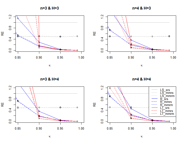
Figure 1: The REs of ${\widehat{\bf\beta}}_{\text{LS}}$, ${\widehat{\bf\beta}}_{\text{R}}$ and ${\widehat{\bf\beta}}_{\text{LT}}$ under SRS, MMRS and MMRM data relative to their ${\widehat{\bf\beta}}_{\text{LS,SRS}}$ counterpart of the same size when $c=1$ with ranking ability $\rho=(1,1,1)$.

In the first simulation, we evaluate the shrinkage estimators for linear regression in the presence of collinearity. We examine how the proposed RSS estimators are affected by sampling parameters, ranking ability and ties information. To simulate the collinearity between predictors, we first generate $u_{ij},i=1,\ldots,N;j=1,\ldots,p+1$ from standard normal distribution. The predictors are generated by

$$x_{i,j}=(1-\kappa^{2})^{1/2}u_{i,j}+\kappa u_{i,p+1}~{}~{}~{}i=1,\ldots,N;j=1,\ldots,p,$$ (27)

where $\kappa$ accounts for the level of collinearity. Here, we consider the multiple regression with four (i.e., $p=4$) predictors ${\bf x}=({x}_{1},{x}_{2},{x}_{3},{x}_{4})$ with nominal correlation levels $\kappa=\{0.85,0.9,0.95,0.99\}$. Using the predictors from (27) and true coefficients ${\bf\beta}_{0}=(0.25,0.25,0.25,0.25)$, we generated the vector of responses as $y_{i}={\bf x}_{i}{\bf\beta}_{0}+\epsilon_{i}$ where $\epsilon_{i};i=1,\ldots,N$ are generated (independently from predictors) from standard normal distribution. There are various proposals for estimation of ridge and Liu parameters for linear regression. As one of the most common approaches, following Hoerl et al. (1975), we obtained the optimal value of $k$ for ridge estimators by ${\widehat{k}}_{\text{HKB}}=p{\hat{\sigma}}/{\bf\beta}^{\top}_{LS}{\bf\beta}_{LS}$. From Kejian (2003), we determined the optimal values of $k$ and $d$ for Liu-type estimators as follows:

$${\widehat{k}}_{\text{LT}}=\frac{\lambda_{1}-100\lambda_{p}}{99},~{}~{}{\widehat{d}}_{\text{LT}}=-\frac{\sum_{j=1}^{p}\lambda_{j}(\widehat{\sigma}^{2}_{R}-{\widehat{k}}_{\text{LT}}{\widehat{\alpha}}^{2}_{R,j})/(\lambda_{j}+{\widehat{k}}_{\text{LT}})^{3}}{\sum_{j=1}^{p}\lambda_{j}(\lambda_{,}{\widehat{\alpha}}^{2}_{R,j}+\widehat{\sigma}^{2}_{R})/(\lambda_{j}+{\widehat{k}}_{\text{LT}})^{4}}$$

where one can obtain ${\widehat{\alpha}}^{2}_{R}=(\Lambda+k\mathbb{I})^{-1}{\bf Z}^{\top}{\bf y}$ and $\widehat{\sigma}^{2}_{R}$ with the estimate of $\sigma^{2}$ from the ridge method.

$n$	$\kappa$	${\widehat{\bf\beta}}_{\text{SRR,SRS}}$	${\widehat{\bf\beta}}_{\text{SRR,MMRS}}$	${\widehat{\bf\beta}}_{\text{SRR,MMRM}}$	${\widehat{\bf\beta}}_{\text{SLR,SRS}}$	${\widehat{\bf\beta}}_{\text{SLR,MMRS}}$	${\widehat{\bf\beta}}_{\text{SLR,MMRM}}$
$3$	0.75	0.528	0.363	0.368	1.231	0.703	0.708
	0.80	0.365	0.283	0.279	1.214	0.746	0.669
	0.85	0.292	0.255	0.256	1.193	0.787	0.703
	0.90	0.259	0.249	0.249	3.229	2.769	4.751
	0.95	0.256	0.252	0.252	266	39.156	49.129
	0.99	0.261	0.257	0.257	0.529	0.949	0.302
$4$	0.75	0.502	0.339	0.336	1.311	0.711	0.714
	0.80	0.337	0.261	0.262	1.281	0.683	0.685
	0.85	0.278	0.248	0.247	1.239	0.648	0.647
	0.90	0.255	0.246	0.246	1.103	0.625	0.586
	0.95	0.255	0.251	0.251	9477	6.208	56.030
	0.99	0.259	0.256	0.256	0.712	0.330	0.361

Table 1: The REs of ${\widehat{\bf\beta}}_{\text{SRR}}$, ${\widehat{\bf\beta}}_{\text{SLR}}$ under SRS, MMRS and MMRM data relative to their ${\widehat{\bf\beta}}_{\text{LS,SRS}}$ counterpart of the same size when $H=3$ and $c=1$ with ranking ability $\rho=(1,1,1)$.

To study the impact of ranking ability, from Dell and Clutter (1972), we generated external observer $R_{l}(l=1,\ldots,K)$ by

$$R_{i,l}=(1-\rho^{2}_{l})^{1/2}y_{i}+\rho u_{i},~{}~{}i=1,\ldots,N;l=1,\ldots,K,$$

where $\rho_{l}=\text{Cor}(R_{l},{\bf y})$ and $u_{i}$ comes from an independent standard normal distribution. In this simulation, we considered three ranking levels $\rho=\{0.5,0.9,1\}$ when we collect MMRS data. In addition, we considered six ranking combinations of $\rho$ to construct MMRM data with two and three observers. The DPS model with tie parameter $c=\{0.5,1,2\}$ were also applied to record the ties information between units in MMRS and MMRM data. Accordingly, we generated $\mathbb{C}=10000$ predictors and responses under SRS, MMRS and MMRM data of the same sizes $N=\{9,12\}$ with set size $H=\{3,4\}$ and calculated the MSE of the estimates as $\text{MSE}({\widehat{\bf\beta}})=1/\mathbb{C}\sum_{l=1}^{\mathbb{C}}({\widehat{\bf\beta}}-{\bf\beta}_{0})^{\top}({\widehat{\bf\beta}}-{\bf\beta}_{0}).$ We compute the efficiency (RE) of shrinkage estimator ${\widehat{\bf\beta}}$ relative to ${\widehat{\bf\beta}}_{\text{LS,SRS}}$ to measure the performance of ${\widehat{\bf\beta}}$. The $\text{RE}({\widehat{\bf\beta}})$ is given by

$$\text{RE}({\widehat{\bf\beta}})=\frac{\text{MSE}({\widehat{\bf\beta}})}{\text{MSE}({\widehat{\bf\beta}}_{\text{LS,SRS}})},$$

where $\text{RE}<1$ indicates the superiority of ${\widehat{\bf\beta}}$ in the estimation of coefficients of regression in the presence of collinearity.

			$n=4,H=6$			$n=2,H=12$
$\phi$	Estimator	Median	2.5%	97.5%	Median	2.5%	97.5%
0.95	${\widehat{\bf\beta}}_{\text{LS,SRS}}$	2657.26	224.40	26303	2511.01	229.39	25043
	${\widehat{\bf\beta}}_{\text{R,SRS}}$	307.39	36.46	3900	285.41	35.66	3353
	${\widehat{\bf\beta}}_{\text{LT,SRS}}$	58.02	11.99	687	54.77	11.46	627
	${\widehat{\bf\beta}}_{\text{LS,RSS}}$	2541.31	266.43	20646	2455.98	242.12	19710
	${\widehat{\bf\beta}}_{\text{R,RSS}}$	287.91	39.35	3624	283.34	37.71	3252
	${\widehat{\bf\beta}}_{\text{LT,RSS}}$	56.51	12.53	701	56.60	11.99	692
	${\widehat{\bf\beta}}_{\text{LS,MRS}}$	2390.56	251.69	20043	2266.78	243.14	19860
	${\widehat{\bf\beta}}_{\text{R,MRS}}$	288.24	38.74	3162	260.80	36.59	2782
	${\widehat{\bf\beta}}_{\text{LT,MRS}}$	56.88	12.47	637	51.22	11.74	597
	${\widehat{\bf\beta}}_{\text{LS,MMR}}$	4334.09	455.25	40774	4065.53	320.09	566201
	${\widehat{\bf\beta}}_{\text{R,MMR}}$	477.85	57.98	4399	439.38	48.57	4805
	${\widehat{\bf\beta}}_{\text{LT,MMR}}$	94.16	15.78	874	84.68	14.05	885
0.98	${\widehat{\bf\beta}}_{\text{LS,SRS}}$	4399.16	320.80	50018	4363.90	307.59	53791
	${\widehat{\bf\beta}}_{\text{R,SRS}}$	308.64	40.60	3509	307.09	39.57	3366
	${\widehat{\bf\beta}}_{\text{LT,SRS}}$	54.59	12.58	663	55.18	12.55	649
	${\widehat{\bf\beta}}_{\text{LS,RSS}}$	4216.01	291.41	43561	4140.31	332.66	44098
	${\widehat{\bf\beta}}_{\text{R,RSS}}$	295.37	40.90	3084	299.80	40.43	3016
	${\widehat{\bf\beta}}_{\text{LT,RSS}}$	53.32	13.29	596	54.13	12.95	577
	${\widehat{\bf\beta}}_{\text{LS,MRS}}$	3941.06	308.70	42562	3909.15	284.66	43700
	${\widehat{\bf\beta}}_{\text{R,MRS}}$	271.68	40.51	2818	293.45	36.41	2996
	${\widehat{\bf\beta}}_{\text{LT,MRS}}$	50.83	12.60	564	52.28	11.96	560
	${\widehat{\bf\beta}}_{\text{LS,MMR}}$	7352.59	551.27	84925	6771.71	438	102627
	${\widehat{\bf\beta}}_{\text{R,MMR}}$	499.72	60.25	4648	457.79	54.14	5065
	${\widehat{\bf\beta}}_{\text{LT,MMR}}$	86.96	16.64	923	79.29	15.32	902

Table 2: The median and 95% CI for the SSE of estimators of coefficients of the logistic model under SRS, RSS, MRS and MMR data of the same size when $\eta=0.95$, $c=0.2$ and ranking ability $(\rho_{1},\rho_{2})=(0.95,0.95)$.

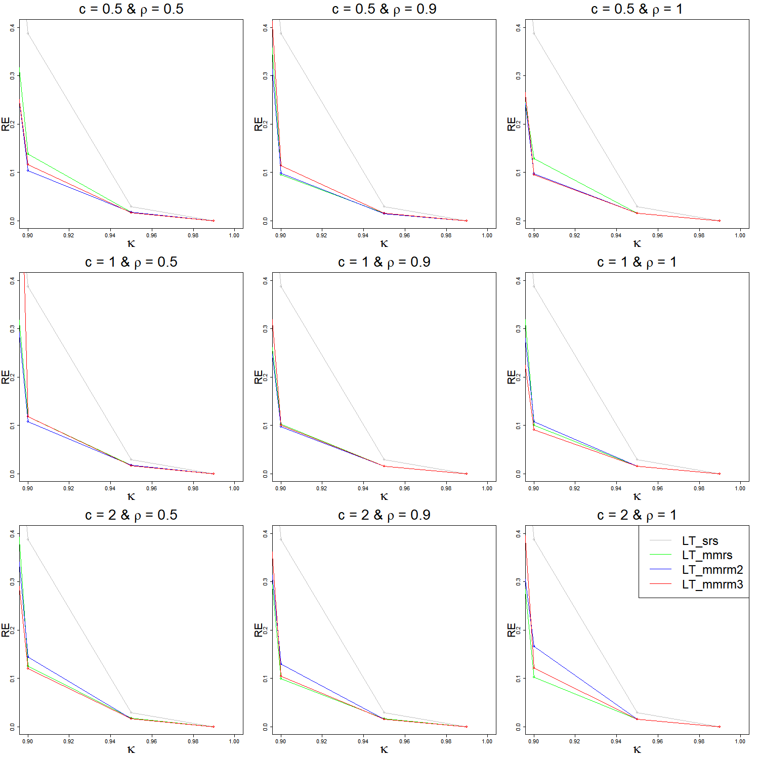
Figure 2: The REs of ${\widehat{\bf\beta}}_{\text{LT}}$ under SRS, RSS, MRS and MMR data relative to their ${\widehat{\bf\beta}}_{\text{LS,SRS}}$ counterpart of the same size when $H=3$ and $n=4$.

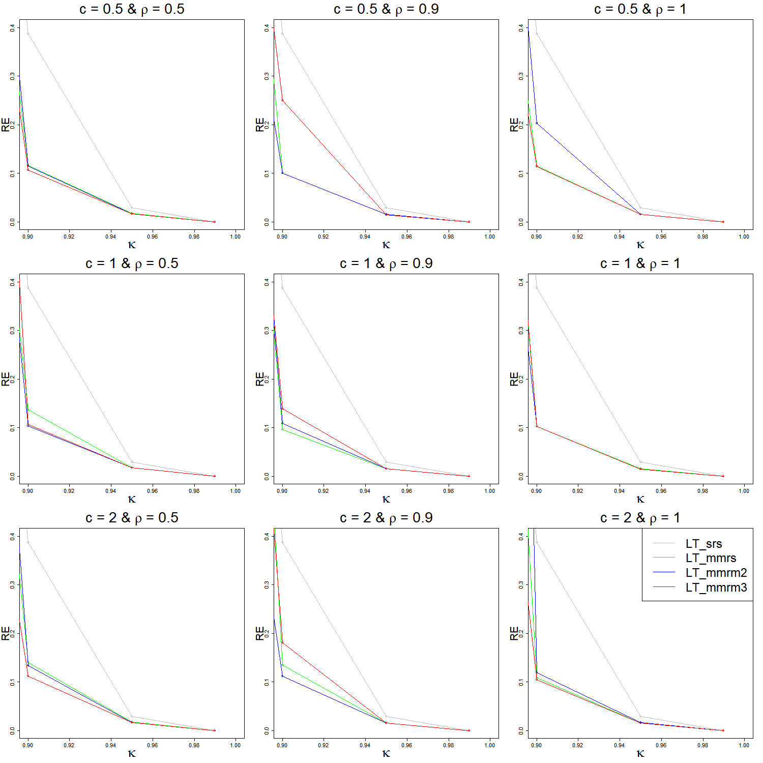
Figure 3: The REs of ${\widehat{\bf\beta}}_{\text{LT}}$ under SRS, RSS, MRS and MMR data relative to their ${\widehat{\bf\beta}}_{\text{LS,SRS}}$ counterpart of the same size when $H=4$ and $n=3$.

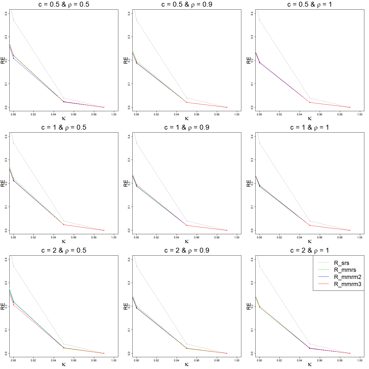
Figure 4: The REs of ${\widehat{\bf\beta}}_{\text{R}}$ under SRS, RSS, MRS and MMR data relative to their ${\widehat{\bf\beta}}_{\text{LS,SRS}}$ counterpart of the same size when $H=3$ and $n=4$.

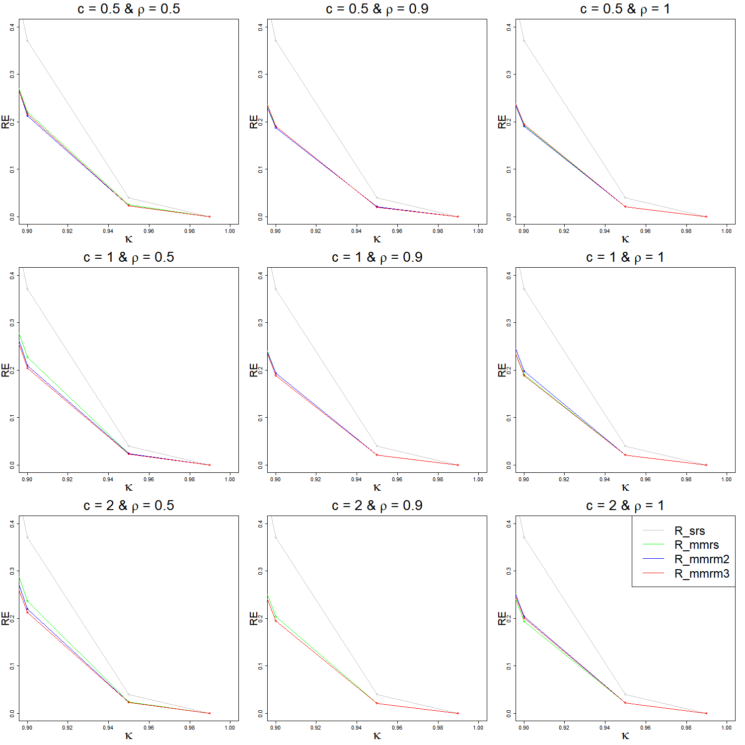
Figure 5: The REs of ${\widehat{\bf\beta}}_{\text{R}}$ under SRS, RSS, MRS and MMR data relative to their ${\widehat{\bf\beta}}_{\text{LS,SRS}}$ counterpart of the same size when $H=4$ and $n=3$.

Figures 1 –5 show the results of this simulation study. It is evident that the biased shrinkage estimators ${\widehat{\bf\beta}}_{\text{R}}$ and ${\widehat{\bf\beta}}_{\text{LT}}$ outperform unbiased estimator ${\widehat{\bf\beta}}_{\text{LS}}$ when the regression model suffers from high collinearity problem. The Liu estimator ${\widehat{\bf\beta}}_{\text{LT,MMRM}}$ shows the best performance when collinearity is sever $(\kappa\geq 0.9)$ while the the ridge estimator ${\widehat{\bf\beta}}_{\text{R,MMRM}}$ is recommended when $\kappa\in[0.85,.9)$. Figures 2 – 5 demonstrate the performance of shrinkage estimators under MMR data with 1, 2 and 3 observers. The efficiency of Liu and Ridge estimators with MMRM data (relative to their counterparts based on MMRS data) improve as the ranking ability $\rho$ increases from $0.5$ to $1$. The RE of multi-observer estimators improve further as the tie parameter $c$ increases from 0.5 to 1; however the RE decreases as $c$ increases from 1 to 2 where many tied ranks are produced in the MMRM data collection.

In the second simulation study, we investigated the performance of SRS, MMRM and MMRS shrinkage estimators for stochastic restricted regression (5). Similar to Arumairajan et al. (2014), we chose the ${\bf\beta}_{0}=(0.6455,0.0896,0.1436,0.1526)$ as the true coefficients of regression model. To implement (5), Similar to Arumairajan et al. (2014), we simulated one restriction with ${\bf R}=(1,-2,-2,-2)$ and ${r}=0$, $v=1$ and generated error term ${\bf e}$ from a normal distribution $N(0,0.0015)$. In addition, we generated the SRS and MMRM and MMRS data and computed the RE of shrinkage estimators (21) and (22) in a similar manner as first simulation study. Tables 1, 5 and 6 show the result of the RE of estimators (21) and (22) based on MMRS and MMRM data when $\kappa\in\{.75,.80,.85,.90,0.95,.99\}$ and tie-parameter $c\in\{.1,.5,1\}$. It is apparent that almost all RSS-based shrinkage estimators outperform their SRS counterparts. Comparing RSS estimators, one observes that the multi-observer methods more efficiently estimate the coefficients of restricted regression in the presence of collinearity than their singe-observer competitors. As reported by Arumairajan et al. (2014), ${\widehat{\bf\beta}}_{\text{SLR}}$ becomes more unstable when collinearity is severe in the model. Therefore, if one has access to multiple decent observers, ${\widehat{\bf\beta}}_{\text{SRR,MMRM}}$ is always recommended to deal with collinearity in restricted regression; otherwise, we recommend ${\widehat{\bf\beta}}_{\text{SLR,MMRS}}$. Interestingly, Table 5 indicates that ${\widehat{\bf\beta}}_{\text{SLR,MMRM}}$ gets more reliable (in the presence of sever collinearity) when more tied ranks are declared in MMRM data collection.

		$n=4,H=6$			$n=2,H=12$
	Median	2.5%	97.5%	Median	2.5%	97.5%
${\widehat{\bf\beta}}_{\text{LS,SRS}}$	0.621	0.273	0.969	0.612	0.265	0.959
${\widehat{\bf\beta}}_{\text{R,SRS}}$	0.136	0.070	0.201	0.136	0.070	0.202
${\widehat{\bf\beta}}_{\text{LT,SRS}}$	0.133	0.071	0.195	0.133	0.070	0.196
${\widehat{\bf\beta}}_{\text{R,RSS}}$	0.136	0.070	0.201	0.136	0.070	0.202
${\widehat{\bf\beta}}_{\text{LT,RSS}}$	0.133	0.070	0.195	0.133	0.071	0.196
${\widehat{\bf\beta}}_{\text{R,MRS}}$	0.136	0.070	0.201	0.136	0.070	0.201
${\widehat{\bf\beta}}_{\text{LT,MRS}}$	0.133	0.070	0.195	0.133	0.071	0.195
${\widehat{\bf\beta}}_{\text{R,MMR}}$	0.131	0.070	0.193	0.129	0.070	0.187
${\widehat{\bf\beta}}_{\text{LT,MMR}}$	0.128	0.070	0.185	0.124	0.070	0.179

Table 3: The Median and 95% CI for the SSE of methods in estimating the bone mineral population via regression model (1) under SRS, RSS, MRS and MMR data of the same size when $c=0.1$.

In the third simulation study, we examine the performance of RSS-based shrinkage methods in estimating the coefficients of logistic regression (12). Similar to Inan and Erdogan (2013), we simulated the logistic regression with $p=4$ predictors where collinearity is incorporated into the model by two parameter $\phi$ and $\eta$. The four predictors are generated by

$$x_{i,j_{1}}=(1-\phi^{2})^{1/2}u_{i,j_{1}}+\phi u_{i,p+1},~{}~{}~{}x_{i,j_{2}}=(1-\eta^{2})^{1/2}u_{i,j_{2}}+\eta u_{i,p+1},$$

where $j_{1}=1,2$ and $j_{2}=3,4$ and errors ${u}_{i,j}$ are generated independently from standard normal distribution. In this simulation, we set the true coefficients of logistic regression as ${\bf\beta}_{0}=(-0.2,1.3,0.8,-0.3,-0.9)$ with $\phi=\{0.95,0.98\}$ and $\eta=\{0.95,0.98\}$. To generate external observers in RSS data collection, we followed the data generation of Zamanzade and Wang (2018). To do so, for a given binary response $y$ and predictors ${\bf x}$, the external observer $R$ is generated as $R|y=0\sim N(0,1)$ and

$$R|y=1\sim N\left(\rho/\sqrt{(1-\rho^{2})g({\bf x},{\bf\beta}_{0})(1-g({\bf x},{\bf\beta}_{0}))},1\right),$$

where $\rho=\text{Cor}(R,y)$ and $g(\cdot)$ is given by (12). We considered $\rho=\{0.75,0.95\}$ to obtain the ranking information in RSS (with single observer), MRS and MMR samples. We also set tie-parameter ${c}={0.2}$ in DPS model to explore the impact of the ties information on the proposed shrinkage estimators. We used the measure $\text{SSE}({\widehat{\bf\beta}})=({\widehat{\bf\beta}}-{\bf\beta}_{0})^{\top}({\widehat{\bf\beta}}-{\bf\beta}_{0})$ to evaluate the performance of coefficient estimate ${\widehat{\bf\beta}}$ in logistic regression with collinearity problem. Accordingly, the shrinkage estimation procedures were replicated 10000 times under SRS, RSS, MRS and MMR data of size $N=24$ with $H=\{6,12\}$. We then computed the median and 95% non-parametric confidence interval (CI) for the SSE of the estimates. The lower and upper bands of each CI were calculated by 2.5 and 97.5 percentiles of the SSEs, respectively.

		$n=4,H=6$			$n=2,H=12$
	Median	2.5%	97.5%	Median	2.5%	97.5%
${\widehat{\bf\beta}}_{\text{LS,SRS}}$	42.47	0.22	982.01	43.08	0.26	821.81
${\widehat{\bf\beta}}_{\text{R,SRS}}$	2.94	0.17	384.88	3.00	0.16	296.15
${\widehat{\bf\beta}}_{\text{LT,SRS}}$	2.38	0.27	40.77	2.38	0.27	37.82
${\widehat{\bf\beta}}_{\text{R,RSS}}$	2.88	0.12	322.69	2.75	0.11	305.16
${\widehat{\bf\beta}}_{\text{LT,RSS}}$	2.38	0.14	38.09	2.38	0.15	33.74
${\widehat{\bf\beta}}_{\text{R,MRS}}$	2.88	0.11	318.75	2.70	0.10	299.59
${\widehat{\bf\beta}}_{\text{LT,MRS}}$	2.38	0.18	37.22	2.38	0.16	36.67

Table 4: The Median and 95% CI for the SSE of methods in the estimation of the bone mineral population via logistic model (12) under SRS, RSS and MRS data of the same size when $c=0.1$.

The results of this simulation study are shown in Tables 2, 7 - 9. Similar to previous simulation studies, the LS estimates are dramatically influenced by collinearity in the logistic regression; unlike LS estimators, there is a significant reduction in the SSE of Liu and ridge estimators. When the collinearity is high, the Liu estimators outperform their ridge competitors in estimating the logistic regression coefficients. Shrinkage estimators based on RSS and MRS data almost always outperform their SRS counterparts. Unlike linear regression where estimators with MMR data were preferred, the RSS and MRS data results in more reliable shrinkage estimates of coefficients of logistic regression. Hence, we only presented the results based on RSS and MRS data for analysis of logistic regression. While the median SSE of ${\widehat{\bf\beta}}_{\text{LT,MRS}}$ and ${\widehat{\bf\beta}}_{\text{LT,RSS}}$ are close, the multi-observer ${\widehat{\bf\beta}}_{\text{LT,MRS}}$ results in the shortest CIs of the SSEs. Interestingly, it is observed that the efficiency of ${\widehat{\bf\beta}}_{\text{LT,MRS}}$ and ${\widehat{\bf\beta}}_{\text{R,MRS}}$ grows further as the collinearity gets more severe in the logistic regression. When the ranking ability is strong, the performance of shrinkage estimators based on RSS and MRS data is improved further as the set size increases. In short, when one has access to multiple observers with decent ranking abilities, ${\widehat{\bf\beta}}_{\text{LT,MRS}}$ is recommended to estimate the coefficients of logistic regression in the presence of collinearity.

6 Bone Mineral Data Analysis

As a bone metabolic disorder problem, osteoporosis happens when the density of the patient’s bone structure decreases considerably. The disease occurs without a major symptom; that is why it is often called a silent thief. There are various characteristics such as sex, age and BMI associated with osteoporosis (Felson et al., 1993, Seeman et al., 1983). Based on the Korean NHANES survey, around 35% of women aged 50 and older in South Korea suffer from osteoporosis while this proportion becomes less than 8% for men in that age group (Lim et al., 2016). In the case of age, it is known that the bone mineral density increases until age 30s and then decreases as the individual ages (Black et al., 1992).

Bone mineral density (BMD) is one of the most reliable factors in determining bone disorder. BMDs, given as T-scores, are compared with a BMD norm to determine the bone disorder status of an individual. If the BMD falls lower than -2.5 SD from the norm, the status is diagnosed as osteoporosis. Although measuring BMD is costly and time-consuming, practitioners have access to several easy-to-measure characteristics about the patients, such as demographic information and BMD scores from previous surveys. We believe practitioners can use a multi-observer RSS scheme, translate these characteristics into ranking information to more efficiently estimate the bone disorder population. Here, we apply RSS, MRS, and MMR samples to analyze bone mineral data obtained from the National Health and Nutritional Examination Survey (NHANES III) conducted with over 33999 American adults by CDC between 1988-1994. The survey includes 241 white women aged 50 and older who participated in two bone examinations. We treat these female participants as our population. Here, we apply the developed shrinkage methods to analyze the BMD data in two numerical studies in the context of linear regression and logistic regression.

In the first study, we considered total BMD (TOBMD) scores from the second bone examination as the response variable of the linear regression. Weight and BMI characteristics were treated as the two predictors of the model where correlation level ${\kappa=.91}$ indicates the collinearity issue in the regression. We treated the TOBMD and INBMD measurements of the first bone examination as two observers with $(\rho_{1},\rho_{2})=(0.97,0.95)$ for ranking purposes. We replicated shrinkage estimates 10000 times under SRS, RSS, MRS and MMR data of size $N=24$ with $H=\{6,12\}$ and $c=0.1$ and computed the median and 95% CI for SSE as described in Section 5. Table 3 illustrates the results of this analysis. Due to the symmetry in linear regression, we see ${\widehat{\bf\beta}}_{\text{LT,MMR}}$ and ${\widehat{\bf\beta}}_{\text{R,MMR}}$ estimate the true coefficients of the bone mineral linear regression more efficiently; hence they are recommend in this analysis. The performance of MMR estimators also improves as the set size increases from 6 to 12 while the sample size remains the same.

Although the population in the second analysis is the same as in the first, we translated the TOMBD scores from the second examination into binary osteoporosis status. We compared the TOBMD of each individual with the TOBMD norm obtained from individuals aged 20-30. If the BMD was larger than -2.5 SD of the norm, we assign $y=1$ (i.e., normal status); otherwise $y=0$ (i.e., osteoporosis status). The TRBMD and FNBMD measurements from the first bone examination with $\kappa=0.80$ were also considered the two predictors of the logistic regression. We ranked the patients with TOBMD and INBMD measurements of the first bone examination as two observers with $(\rho_{1},\rho_{2})=(0.97,0.96)$. Similar to the first analysis, we computed the median and 95% CI for SSE of shrinkage estimators based on SRS, RSS and MRS samples of size $N=24$ with $H=\{6,12\}$ and $c=0.1$. The results are shown in Table 4. The shrinkage methods result in a considerable reduction in the length of CIs for SSEs in the presence of collinearity. We also see that the RSS and MRS shrinkage estimators almost always outperform the SRS estimators. Similar to the first analysis, when practitioners have access to decent observers, the performance of RSS-based shrinkage estimators can be improved as the set size increases.

7 Summary and Concluding Remarks

In many applications such as osteoporosis research, measuring the variable of interest is obtained through an expensive and time-consuming process; however, practitioners have access to many inexpensive and easy-to-measure characteristics about the individuals. In these situations, ranked set sampling, as an alternative to commonly-used simple random sampling, can translate these characteristics into data collection, providing more representative samples from the population. Collinearity is a common challenge in linear models that leads to unreliable coefficient estimates under the least square method and consequently misleading information. Ebegil et al. (2021) recently proposed ridge and Liu-type estimates under RSS data to handle the collinearity; however, the developed RSS estimators can not enjoy multiple ranking sources and ties information in data collection. Despite the importance of logistic regression in medical studies, no research has investigated the RSS shrinkage estimators to deal with the collinearity in logistic regression and stochastic restricted regression. In this manuscript, we developed the Liu-type and ridge estimation methods under multi-observer RSS data to estimate the coefficients of the linear regression, stochastic restricted regression and logistic regression in the presence of collinearity. When the collinearity level is high and practitioners have access to multiple decent observers, the ${\widehat{\bf\beta}}_{\text{LT,MMRM}}$ is recommended to handle the estimation problem in linear regression and stochastic restricted regression models. In the case of high collinearity in the logistic regression model, ${\widehat{\bf\beta}}_{\text{LT,MRS}}$ shows the most reliable coefficient estimates.

8 Appendix

8.1 Proof of Lemma 1

$$\mathbb{E}({\widehat{\bf\beta}}_{\text{LS,MRS}})={\bf S}^{-1}_{\text{MRS}}{\bf X}_{\text{MRS}}\mathbb{E}({\bf y}_{\text{MRS}}|{\bf X}_{\text{MRS}})={\bf S}^{-1}_{\text{MRS}}{\bf X}_{\text{MRS}}{\bf X}^{\top}_{\text{MRS}}{\bf\beta}=\beta.$$

$$\text{Var}({\widehat{\bf\beta}}_{\text{LS,MRS}})=\text{Var}({\bf S}^{-1}_{\text{MRS}}{\bf X}_{\text{MRS}}{\bf y}_{\text{MRS}})={\bf S}^{-1}_{\text{MRS}}{\bf X}_{\text{MRS}}\text{Var}({\bf y}_{\text{MRS}}|{\bf X}_{\text{MRS}}){\bf X}^{\top}_{\text{MRS}}{\bf S}^{-1}_{\text{MRS}}=\sigma^{2}{\bf S}^{-1}_{\text{MRS}}.$$

The proof is completed by the property of concomitant of order statistics where $\mathbb{E}({\bf y}_{\text{MRS}}|{\bf X}_{\text{MRS}})=\mathbb{E}({\bf y}|{\bf X})$ and the fact that RSS data are independent statistics. $\square$

8.2 Proof of Lemma 2

One can easily rewrite the ridge estimator as follows

$${\widehat{\bf\beta}}_{\text{R,MRS}}=(\mathbb{I}+k{\bf S}^{-1}_{\text{MRS}})^{-1}{\widehat{\bf\beta}}_{\text{LS,MRS}}.$$ (28)

From (28) and Lemma 1, one can easily complete the proof. $\square$

8.3 Proof of Lemma 3

We can rewrite the Liu estimator as follows

$${\widehat{\bf\beta}}_{\text{LT,MRS}} =({\bf S}_{\text{MRS}}+k\mathbb{I})^{-1}({\bf X}_{\text{MRS}}^{\top}{\bf y}_{\text{MRS}}+d{\widehat{\bf\beta}}_{\text{R,MRS}})$$

$$=({\bf S}_{\text{MRS}}+k\mathbb{I})^{-1}\left(\mathbb{I}+d({\bf S}_{\text{MRS}}+k\mathbb{I})^{-1}\right){\bf S}_{\text{MRS}}{\widehat{\bf\beta}}_{\text{LS,MRS}}$$

$$={\bf A}_{\text{LT,MRS}}{\widehat{\bf\beta}}_{\text{LS,MRS}}.$$ (29)

Now from (8.3) and Lemma 1, one can easily complete the proof. $\square$

8.4 Proof of Lemma 5

• From restriction model 5 and $\text{Var}({\bf e})=\sigma^{2}{\bf\Omega}$, the penalized sum of least squares becomes

  $${Q}_{\text{MRS}}=({\bf y}_{\text{MRS}}-{\bf X}_{\text{MRS}}{\bf\beta})^{\top}({\bf y}_{\text{MRS}}-{\bf X}_{\text{MRS}}{\bf\beta})+v({\bf\Omega}^{-1/2}{\bf r}-{\bf\Omega}^{-1/2}{\bf R}{\bf\beta})^{\top}({\bf\Omega}^{-1/2}{\bf r}-{\bf\Omega}^{-1/2}{\bf R}{\bf\beta}).$$ (30)

  From (30), it is easy to prove part (i).

• $${\widehat{\bf\beta}}_{\text{ME,MRS}} =({\bf S}_{\text{MRS}}+v{\bf R}^{\top}{\bf\Omega}^{-1}{\bf R})^{-1}({\bf X}_{\text{MRS}}^{\top}{\bf y}_{\text{MRS}}+v{\bf R}^{\top}{\bf\Omega}^{-1}{\bf r})$$

  $$=({\bf S}_{\text{MRS}}+v{\bf R}^{\top}{\bf\Omega}^{-1}{\bf R})^{-1}{\bf X}_{\text{MRS}}^{\top}{\bf y}_{\text{MRS}}+({\bf S}_{\text{MRS}}+v{\bf R}^{\top}{\bf\Omega}^{-1}v{\bf R}^{\top}{\bf\Omega}^{-1}{\bf r})$$

  $$=\left({\bf S}_{\text{MRS}}^{-1}+v{\bf S}_{\text{MRS}}^{-1}{\bf R}^{\top}({\bf\Omega}+v{\bf R}{\bf\Omega}^{-1}{\bf R}^{\top})^{-1}{\bf R}{\bf S}_{\text{MRS}}^{-1}\right){\bf X}_{\text{MRS}}^{\top}{\bf y}_{\text{MRS}}$$

  $$~{}~{}~{}~{}+v{\bf S}_{\text{MRS}}^{-1}{\bf R}^{\top}({\bf\Omega}+v{\bf R}{\bf\Omega}^{-1}{\bf R}^{\top})^{-1}{\bf r}$$

  $$={\bf S}_{\text{MRS}}^{-1}{\bf X}_{\text{MRS}}^{\top}{\bf y}_{\text{MRS}}-v{\bf S}_{\text{MRS}}^{-1}{\bf R}^{\top}({\bf\Omega}+v{\bf R}{\bf\Omega}^{-1}{\bf R}^{\top})^{-1}{\bf R}{\bf S}_{\text{MRS}}^{-1}{\bf X}_{\text{MRS}}^{\top}{\bf y}_{\text{MRS}}$$

  $$~{}~{}~{}~{}+v{\bf S}_{\text{MRS}}^{-1}{\bf R}^{\top}({\bf\Omega}+v{\bf R}{\bf\Omega}^{-1}{\bf R}^{\top})^{-1}{\bf r}$$

  $$={\widehat{\bf\beta}}_{\text{LS,MRS}}+v{\bf S}_{\text{MRS}}^{-1}{\bf R}^{\top}({\bf\Omega}+v{\bf R}{\bf\Omega}^{-1}{\bf R}^{\top})^{-1}\left({\bf r}-{\bf R}{\bf S}_{\text{MRS}}^{-1}{\bf X}_{\text{MRS}}^{\top}{\bf y}_{\text{MRS}}\right)$$

  $$={\widehat{\bf\beta}}_{\text{LS,MRS}}+v{\bf S}_{\text{MRS}}^{-1}{\bf R}^{\top}({\bf\Omega}+v{\bf R}{\bf\Omega}^{-1}{\bf R}^{\top})^{-1}\left({\bf r}-{\bf R}{\widehat{\bf\beta}}_{\text{LS,MRS}}\right),$$

  where the third equality is implied by Lemma 4. $\square$

8.5 Proof of Lemma 6

Let ${\bf F}_{{\text{MRS}},d}=({\bf S}_{\text{MRS}}+\mathbb{I})^{-1}({\bf S}_{\text{MRS}}+d\mathbb{I})$. We first show

$${\widehat{\bf\beta}}_{\text{LT1,MRS}} =({\bf S}_{\text{MRS}}+\mathbb{I})^{-1}({\bf X}_{\text{MRS}}^{\top}{\bf y}_{\text{MRS}}+d{\widehat{\bf\beta}}_{\text{LS,MRS}})$$

$$=({\bf S}_{\text{MRS}}+\mathbb{I})^{-1}({\bf S}_{\text{MRS}}{\widehat{\bf\beta}}_{\text{LS,MRS}}+d{\widehat{\bf\beta}}_{\text{LS,MRS}})$$

$$={\bf F}_{{\text{MRS}},d}{\bf S}_{\text{MRS}}^{-1}{\bf X}_{\text{MRS}}^{\top}{\bf y}_{\text{MRS}}.$$ (31)

From (8.5) and (22) and that ${\bf F}_{{\text{MRS}},d}$ and ${\bf S}_{\text{MRS}}^{-1}$ are commutative, we derive ${\widehat{\bf\beta}}_{\text{SRL,MRS}}$ as follows

$${\widehat{\bf\beta}}_{\text{SRL,MRS}} ={\bf S}_{\text{MRS}}^{-1}{\bf F}_{{\text{MRS}},d}{\bf X}_{\text{MRS}}^{\top}{\bf y}_{\text{MRS}}+v{\bf S}_{\text{MMR}}^{-1}{\bf R}^{\top}({\bf\Omega}+v{\bf R}{\bf S}_{\text{MMR}}^{-1}{\bf R}^{\top})^{-1}({\bf r}-{\bf R}{\bf S}_{\text{MRS}}^{-1}{\bf F}_{{\text{MRS}},d}{\bf X}_{\text{MRS}}^{\top}{\bf y}_{\text{MRS}})$$

$$={\bf S}_{\text{MRS}}^{-1}{\bf F}_{{\text{MRS}},d}{\bf X}_{\text{MRS}}^{\top}{\bf y}_{\text{MRS}}+v{\bf S}_{\text{MMR}}^{-1}{\bf R}^{\top}({\bf\Omega}+v{\bf R}{\bf S}_{\text{MMR}}^{-1}{\bf R}^{\top})^{-1}{\bf r}$$

$$~{}~{}-v{\bf S}_{\text{MMR}}^{-1}{\bf R}^{\top}({\bf\Omega}+v{\bf R}{\bf S}_{\text{MMR}}^{-1}{\bf R}^{\top})^{-1}{\bf R}{\bf S}_{\text{MRS}}^{-1}{\bf F}_{{\text{MRS}},d}{\bf X}_{\text{MRS}}^{\top}{\bf y}_{\text{MRS}}$$

$$=\left({\bf S}_{\text{MRS}}^{-1}-v{\bf S}_{\text{MMR}}^{-1}{\bf R}^{\top}({\bf\Omega}+v{\bf R}{\bf S}_{\text{MMR}}^{-1}{\bf R}^{\top})^{-1}{\bf R}{\bf S}_{\text{MRS}}^{-1}\right)\left({\bf F}_{{\text{MRS}},d}{\bf X}_{\text{MRS}}^{\top}{\bf y}_{\text{MRS}}+v{\bf R}^{\top}{\bf\Omega}^{-1}{\bf r}\right)$$

$$=({\bf S}_{\text{MRS}}+v{\bf R}^{\top}{\bf\Omega}^{-1}{\bf R})^{-1}({\bf F}_{{\text{MRS}},d}{\bf X}_{\text{MRS}}^{\top}{\bf y}_{\text{MRS}}+v{\bf R}^{\top}{\bf\Omega}^{-1}{\bf r}).$$ (32)

From (8.5) and Lemma 1, the expected value of ${\widehat{\bf\beta}}_{\text{SRL,MRS}}$ yields

$$\mathbb{E}({\widehat{\bf\beta}}_{\text{SRL,MRS}}) =({\bf S}_{\text{MRS}}+v{\bf R}^{\top}{\bf\Omega}^{-1}{\bf R})^{-1}{\bf F}_{{\text{MRS}},d}{\bf X}_{\text{MRS}}^{\top}\mathbb{E}({\bf y}_{\text{MRS}}|{\bf X}_{\text{MRS}})+({\bf S}_{\text{MRS}}+v{\bf R}^{\top}{\bf\Omega}^{-1}{\bf R})^{-1}v{\bf R}^{\top}{\bf\Omega}^{-1}\mathbb{E}({\bf r})$$

$$={\bf\beta}+({\bf S}_{\text{MRS}}+v{\bf R}^{\top}{\bf\Omega}^{-1}{\bf R})^{-1}({\bf F}_{{\text{MRS}},d}-\mathbb{I}){\bf S}_{\text{MRS}}{\bf\beta}.$$

$$\text{Var}({\widehat{\bf\beta}}_{\text{SRL,MRS}}) ={\bf A}_{\text{SRL,MRS}}{\bf F}_{{\text{MRS}},d}{\bf X}_{\text{MRS}}^{\top}\text{Var}({\bf y}_{\text{MRS}}|{\bf X}_{\text{MRS}}){\bf X}_{\text{MRS}}{\bf F}_{{\text{MRS}},d}^{\top}{\bf A}_{\text{SRL,MRS}}$$

$$~{}~{}+v^{2}{\bf A}_{\text{SRL,MRS}}{\bf R}^{\top}{\bf\Omega}^{-1}\text{Var}({\bf r}){\bf\Omega}^{-1}{\bf R}{\bf A}_{\text{SRL,MRS}}$$

$$=\sigma^{2}{\bf A}_{\text{SRL,MRS}}\left({\bf F}_{{\text{MRS}},d}{\bf S}_{\text{MRS}}{\bf F}_{{\text{MRS}},d}^{\top}+v^{2}{\bf R}^{\top}{\bf\Omega}^{-1}{\bf R}\right){\bf A}_{\text{SRL,MRS}},$$

where ${\bf A}_{\text{SRL,MRS}}=({\bf S}_{\text{MRS}}+v{\bf R}^{\top}{\bf\Omega}^{-1}{\bf R})^{-1}$ and the first equality is implied by (8.5) and Lemma 1. $\square$

8.6 Proof of Lemma 7

Let ${\bf W}_{\text{MRS}}=(\mathbb{I}+k{\bf S}_{\text{MRS}}^{-1})^{-1}$. From (28) and that fact that ${\bf W}_{\text{MRS}}$ and ${\bf S}_{\text{MRS}}^{-1}$ are commutative, we show

$${\widehat{\bf\beta}}_{\text{SRR,MRS}} ={\bf W}_{\text{MRS}}{\widehat{\bf\beta}}_{\text{LS,MRS}}+v{\bf S}_{\text{MRS}}^{-1}{\bf R}^{\top}({\bf\Omega}+v{\bf R}{\bf S}_{\text{MRS}}^{-1}{\bf R}^{\top})^{-1}({\bf r}-{\bf R}{\bf W}_{\text{MRS}}{\widehat{\bf\beta}}_{\text{LS,MRS}})$$

$$={\bf S}_{\text{MRS}}^{-1}{\bf W}_{\text{MRS}}{\bf X}_{\text{MRS}}^{\top}{\bf y}_{\text{MRS}}+v{\bf S}_{\text{MRS}}^{-1}{\bf R}^{\top}({\bf\Omega}+v{\bf R}{\bf S}_{\text{MRS}}^{-1}{\bf R}^{\top})^{-1}({\bf r}-{\bf R}{\bf S}_{\text{MRS}}^{-1}{\bf W}_{\text{MRS}}{\bf X}_{\text{MRS}}^{\top}{\bf y}_{\text{MRS}})$$

$$=\left({\bf S}_{\text{MRS}}^{-1}-v{\bf S}_{\text{MMR}}^{-1}{\bf R}^{\top}({\bf\Omega}+v{\bf R}{\bf S}_{\text{MMR}}^{-1}{\bf R}^{\top})^{-1}{\bf R}{\bf S}_{\text{MRS}}^{-1}\right)\left({\bf W}_{\text{MRS}}{\bf X}_{\text{MRS}}^{\top}{\bf y}_{\text{MRS}}+v{\bf R}^{\top}{\bf\Omega}^{-1}{\bf r}\right)$$

$$=({\bf S}_{\text{MRS}}+v{\bf R}^{\top}{\bf\Omega}^{-1}{\bf R})^{-1}\left({\bf W}_{\text{MRS}}{\bf X}_{\text{MRS}}^{\top}{\bf y}_{\text{MRS}}+v{\bf R}^{\top}{\bf\Omega}^{-1}{\bf r}\right).$$ (33)

Using 8.6 and Lemma 1, we compute the expected value of ${\widehat{\bf\beta}}_{\text{SRR,MRS}}$ as

$$\mathbb{E}({\widehat{\bf\beta}}_{\text{SRR,MRS}}) =({\bf S}_{\text{MRS}}+v{\bf R}^{\top}{\bf\Omega}^{-1}{\bf R})^{-1}{\bf W}_{\text{MRS}}{\bf X}_{\text{MRS}}^{\top}\mathbb{E}({\bf y}_{\text{MRS}}|{\bf X}_{\text{MRS}})+({\bf S}_{\text{MRS}}+v{\bf R}^{\top}{\bf\Omega}^{-1}{\bf R})^{-1}v{\bf R}^{\top}{\bf\Omega}^{-1}\mathbb{E}({\bf r})$$

$$=({\bf S}_{\text{MRS}}+v{\bf R}^{\top}{\bf\Omega}^{-1}{\bf R})^{-1}{\bf W}_{\text{MRS}}{\bf S}_{\text{MRS}}{\bf\beta}+({\bf S}_{\text{MRS}}+v{\bf R}^{\top}{\bf\Omega}^{-1}{\bf R})^{-1}v{\bf R}^{\top}{\bf\Omega}^{-1}{\bf R})^{-1}v{\bf R}^{\top}{\bf\Omega}^{-1}{\bf R}{\bf\beta}$$

$$={\bf\beta}+({\bf S}_{\text{MRS}}+v{\bf R}^{\top}{\bf\Omega}^{-1}{\bf R})^{-1}\left({\bf W}_{\text{MRS}}-\mathbb{I}\right){\bf S}_{\text{MRS}}{\bf\beta}.$$

$$\text{Var}({\widehat{\bf\beta}}_{\text{SRR,MRS}}) ={\bf A}_{\text{SRR,MSR}}{\bf W}_{\text{MRS}}{\bf X}_{\text{MRS}}^{\top}\text{Var}({\bf y}_{\text{MRS}}|{\bf X}_{\text{MRS}}){\bf X}_{\text{MRS}}{\bf W}_{\text{MRS}}^{\top}{\bf A}_{\text{SRR,MSR}}$$

$$~{}~{}+v^{2}{\bf A}_{\text{SRR,MSR}}{\bf R}^{\top}{\bf\Omega}^{-1}\text{Var}({\bf r}){\bf\Omega}^{-1}{\bf R}{\bf A}_{\text{SRR,MSR}}$$

$$=\sigma^{2}{\bf A}_{\text{SRR,MSR}}\left({\bf W}_{\text{MRS}}{\bf S}_{\text{MRS}}{\bf W}_{\text{MRS}}^{\top}+v^{2}{\bf R}^{\top}{\bf\Omega}^{-1}{\bf R}\right){\bf A}_{\text{SRR,MSR}},$$

where ${\bf A}_{\text{SRR,MSR}}=({\bf S}_{\text{MRS}}+v{\bf R}^{\top}{\bf\Omega}^{-1}{\bf R})^{-1}$ and the first equality is implied by (8.6) and Lemma 1. $\square$

$n$	$\kappa$	${\widehat{\bf\beta}}_{\text{SMRE,SRS}}$	${\widehat{\bf\beta}}_{\text{SMRE,MMRS}}$	${\widehat{\bf\beta}}_{\text{SMRE,MMRM}}$	${\widehat{\bf\beta}}_{\text{SLE,SRS}}$	${\widehat{\bf\beta}}_{\text{SLE,MMRS}}$	${\widehat{\bf\beta}}_{\text{SLE,MMRM}}$
3	0.75	0.493	0.342	0.339	1.289	0.723	0.721
	0.80	0.334	0.263	0.262	1.284	0.691	0.682
	0.85	0.277	0.247	0.247	1.245	0.648	0.663
	0.90	0.254	0.246	0.245	1.248	0.600	0.580
	0.95	0.255	0.250	0.251	14.079	2.923	17.492
	0.99	0.259	0.256	0.256	0.296	0.441	0.321
4	0.75	0.439	0.304	0.308	1.235	0.692	0.695
	0.80	0.308	0.243	0.243	1.269	0.667	0.656
	0.85	0.264	0.239	0.239	1.246	0.624	0.626
	0.90	0.251	0.244	0.244	1.109	0.569	0.566
	0.95	0.253	0.250	0.250	14.108	163	63.751
	0.99	0.257	0.255	0.255	0.434	11.426	0.623

Table 5: The REs of ${\widehat{\bf\beta}}_{\text{SMRE}}$, ${\widehat{\bf\beta}}_{\text{SLE}}$ under SRS, MRS and MMR data relative to their ${\widehat{\bf\beta}}_{\text{LS,SRS}}$ counterpart of the same size when $H=4$ and $c=1$ with ranking ability $\rho=(1,1,1)$.

$\kappa$	$c$	${\widehat{\bf\beta}}_{\text{SMRE,SRS}}$	${\widehat{\bf\beta}}_{\text{SMRE,MMR}}$	${\widehat{\bf\beta}}_{\text{SLE,SRS}}$	${\widehat{\bf\beta}}_{\text{SLE,MMR}}$
0.75	0.1	0.48638	0.31411	1.27164	0.63137
	0.5	0.49507	0.32370	1.28471	0.65129
	1.0	0.49255	0.33905	1.28901	0.72098
0.8	0.1	0.33630	0.24889	1.29035	0.59610
	0.5	0.33329	0.25168	1.26088	0.62620
	1	0.33432	0.26249	1.28387	0.68222
0.85	0.1	0.27714	0.24186	1.21881	0.55860
	0.5	0.27704	0.24341	1.24289	0.58399
	1	0.27666	0.24701	1.24523	0.66252
0.9	0.1	0.25451	0.24411	1.08373	5.34304
	0.5	0.25400	0.24514	1.64597	0.69039
	1	0.25430	0.24524	1.24823	0.58050
0.95	0.1	0.25421	0.24995	59.38280	558.768
	0.5	0.25493	0.25037	36.05183	13.2592
	1	0.25478	0.25094	14.07878	17.4918
0.99	0.1	0.25864	0.25519	0.56044	0.55860
	0.5	0.25869	0.25536	7.37324	0.58399
	1	0.25929	0.25602	0.29642	0.66252

Table 6: The REs of ${\widehat{\bf\beta}}_{\text{SMRE}}$, ${\widehat{\bf\beta}}_{\text{SLE}}$ under SRS and MMR data relative to their ${\widehat{\bf\beta}}_{\text{LS,SRS}}$ counterpart of the same size with $N=12$, $H=4$ with ranking ability $\rho=(1,1,1)$.

			$n=4,H=6$			$n=2,H=12$
$\phi$	Estimator	Median	2.5%	97.5%	Median	2.5%	97.5%
0.95	${\widehat{\bf\beta}}_{\text{LS,SRS}}$	8146.35	350.71	141588	8335.14	330.48	137471
	${\widehat{\bf\beta}}_{\text{R,SRS}}$	478.35	42.25	7093	492.66	37.17	7163
	${\widehat{\bf\beta}}_{\text{LT,SRS}}$	76.23	12.82	1083	78.70	12.40	1058
	${\widehat{\bf\beta}}_{\text{LS,RSS}}$	8018.13	314.70	113177	7781.22	346.63	119211
	${\widehat{\bf\beta}}_{\text{R,RSS}}$	482.96	41.18	6417	466.35	42.86	6490
	${\widehat{\bf\beta}}_{\text{LT,RSS}}$	77.57	12.65	1015	74.71	13.11	1072
	${\widehat{\bf\beta}}_{\text{LS,MRS}}$	7749.11	356.69	104580	7269.18	308.65	104153
	${\widehat{\bf\beta}}_{\text{R,MRS}}$	474.22	41.78	5760	448.40	41.62	5998
	${\widehat{\bf\beta}}_{\text{LT,MRS}}$	76.74	13.18	997	72.81	12.72	1009
0.98	${\widehat{\bf\beta}}_{\text{LS,SRS}}$	12316.19	565.68	158677	12137.58	570.44	150771
	${\widehat{\bf\beta}}_{\text{R,SRS}}$	364.46	45.09	6921	341.25	42.22	6693
	${\widehat{\bf\beta}}_{\text{LT,SRS}}$	58.22	13.95	808	56.22	13.09	793
	${\widehat{\bf\beta}}_{\text{LS,RSS}}$	12252.13	559.89	142438	12145.12	580.39	133728
	${\widehat{\bf\beta}}_{\text{R,RSS}}$	350.58	44.49	6747	341.58	45.47	6232
	${\widehat{\bf\beta}}_{\text{LT,RSS}}$	56.44	13.92	817	56.12	13.93	731
	${\widehat{\bf\beta}}_{\text{LS,MRS}}$	11925.81	593.71	129248	11453.22	582.81	124213
	${\widehat{\bf\beta}}_{\text{R,MRS}}$	349.00	42.52	6485	336.47	43.31	6525
	${\widehat{\bf\beta}}_{\text{LT,MRS}}$	55.47	13.49	723	54.69	13.69	751

Table 7: The median and 95% CI for the MSE of estimators of coefficients of the logistic model under SRS, RSS, MRS and MMR data of the same size when $\eta=0.98$, $c=0.2$ and ranking ability $\rho=(0.95,0.95)$.

			$n=4,H=6$			$n=2,H=12$
$\phi$	Estimator	Median	2.5%	97.5%	Median	2.5%	97.5%
0.95	${\widehat{\bf\beta}}_{\text{LS,SRS}}$	2635.56	237.25	23294	2660.21	246.47	24389
	${\widehat{\bf\beta}}_{\text{R,SRS}}$	299.16	38.18	3802	294.72	39.02	3396
	${\widehat{\bf\beta}}_{\text{LT,SRS}}$	58.17	12.06	670	56.79	12.15	710
	${\widehat{\bf\beta}}_{\text{LS,RSS}}$	2635.15	238.40	20987	2480.01	235.60	21816
	${\widehat{\bf\beta}}_{\text{R,RSS}}$	309.76	37.36	3616	284.17	37.01	3946
	${\widehat{\bf\beta}}_{\text{LT,RSS}}$	59.91	12.02	706	57.44	12.03	688
	${\widehat{\bf\beta}}_{\text{LS,MRS}}$	2503.00	245.12	21639	2468.72	235.50	23036
	${\widehat{\bf\beta}}_{\text{R,MRS}}$	293.57	38.41	3101	280.75	37.58	4192
	${\widehat{\bf\beta}}_{\text{LT,MRS}}$	57.30	11.97	632	54.59	12.10	785
0.98	${\widehat{\bf\beta}}_{\text{LS,SRS}}$	4410.32	327.17	55437	4214.86	309.32	50111
	${\widehat{\bf\beta}}_{\text{R,SRS}}$	324.51	38.93	3423	303.68	39.87	3315
	${\widehat{\bf\beta}}_{\text{LT,SRS}}$	56.98	12.89	657	53.69	13.09	631
	${\widehat{\bf\beta}}_{\text{LS,RSS}}$	4354.90	340.09	43784	4298.78	353.43	46839
	${\widehat{\bf\beta}}_{\text{R,RSS}}$	321.45	42.36	3285	313.95	43.35	3343
	${\widehat{\bf\beta}}_{\text{LT,RSS}}$	57.78	13.34	605	55.79	13.35	668
	${\widehat{\bf\beta}}_{\text{LS,MRS}}$	4240.66	295.37	45573	4386.70	328.58	46921
	${\widehat{\bf\beta}}_{\text{R,MRS}}$	307.44	37.60	3429	310.22	40.33	3313
	${\widehat{\bf\beta}}_{\text{LT,MRS}}$	54.32	12.23	659	55.08	12.95	633

Table 8: The median and 95% CI for the MSE of estimators of coefficients of the logistic model under SRS, RSS, MRS and MMR data of the same size when $\eta=0.95$, $c=0.2$ and ranking ability $\rho=(0.5,0.5)$.

			$n=4,H=6$			$n=2,H=12$
$\phi$	Estimator	Median	2.5%	97.5%	Median	2.5%	97.5%
0.95	${\widehat{\bf\beta}}_{\text{LS,SRS}}$	8186.92	322.25	147400	8200.18	284.92	128528
	${\widehat{\bf\beta}}_{\text{R,SRS}}$	472.71	41.20	7086	470.02	38.31	6824
	${\widehat{\bf\beta}}_{\text{LT,SRS}}$	76.43	13.00	1111	73.79	12.58	1082
	${\widehat{\bf\beta}}_{\text{LS,RSS}}$	8106.87	304.24	116801	8372.63	372.34	114303
	${\widehat{\bf\beta}}_{\text{R,RSS}}$	467.80	39.51	6718	503.27	42.88	6466
	${\widehat{\bf\beta}}_{\text{LT,RSS}}$	76.01	12.91	1002	80.10	13.26	1119
	${\widehat{\bf\beta}}_{\text{LS,MRS}}$	7822.96	331.31	112281	7956.18	295.11	120813
	${\widehat{\bf\beta}}_{\text{R,MRS}}$	459.36	42.74	6587	476.00	39.83	6582
	${\widehat{\bf\beta}}_{\text{LT,MRS}}$	73.70	13.08	1056	76.28	12.58	1058
0.98	${\widehat{\bf\beta}}_{\text{LS,SRS}}$	12461.70	573.95	152708	12285.95	535.29	164743
	${\widehat{\bf\beta}}_{\text{R,SRS}}$	360.71	45.37	6604	334.03	41.14	7232
	${\widehat{\bf\beta}}_{\text{LT,SRS}}$	58.11	13.86	758	55.56	13.04	866
	${\widehat{\bf\beta}}_{\text{LS,RSS}}$	12874.86	685.43	146421	12784.51	535.32	146359
	${\widehat{\bf\beta}}_{\text{R,RSS}}$	372.82	46.75	6818	376.91	43.59	6699
	${\widehat{\bf\beta}}_{\text{LT,RSS}}$	59.06	13.92	779	59.20	13.61	806
	${\widehat{\bf\beta}}_{\text{LS,MRS}}$	12198.05	550.33	129290	11936.86	521.83	141357
	${\widehat{\bf\beta}}_{\text{R,MRS}}$	361.00	42.29	6790	352.16	41.51	6422
	${\widehat{\bf\beta}}_{\text{LT,MRS}}$	57.81	13.10	773	56.68	13.33	725

Table 9: The median and 95% CI for the MSE of estimators of coefficients of the logistic model under SRS, RSS, MRS and MMR data of the same size when $\eta=0.98$, $c=0.2$ and ranking ability $\rho=(0.5,0.5)$.

References

- Alvandi and Hatefi (2021) Amirhossein Alvandi and Armin Hatefi. Estimation of ordinal population with multi-observer ranked set samples using ties information. Statistical Methods in Medical Research, 2021.
- Amiri et al. (2014) Saeid Amiri, Mohammad Jafari Jozani, and Reza Modarres. Resampling unbalanced ranked set samples with applications in testing hypothesis about the population mean. Journal of agricultural, biological, and environmental statistics, 19(1):1–17, 2014.
- Arumairajan et al. (2014) Sivarajah Arumairajan, Pushpakanthie Wijekoon, et al. Improvement of ridge estimator when stochastic restrictions are available in the linear regression model. Journal of Statistical and Econometric Methods, 3(1):35–48, 2014.
- Black et al. (1992) Dennis M Black, Steven R Cummings, Harry K Genant, Michael C Nevitt, Lisa Palermo, and Warren Browner. Axial and appendicular bone density predict fractures in older women. Journal of Bone and Mineral Research, 7(6):633–638, 1992.
- Bliuc et al. (2009) Dana Bliuc, Nguyen D Nguyen, Vivienne E Milch, Tuan V Nguyen, and John A Eisman. Mortality risk associated with low-trauma osteoporotic fracture and subsequent fracture in men and women. Jama, 301(5):513–521, 2009.
- Chen et al. (2005) Haiying Chen, Elizabeth A Stasny, and Douglas A Wolfe. Ranked set sampling for efficient estimation of a population proportion. Statistics in medicine, 24(21):3319–3329, 2005.
- Cummings et al. (1995) Steven R Cummings, Michael C Nevitt, Warren S Browner, Katie Stone, Kathleen M Fox, Kristine E Ensrud, Jane Cauley, Dennis Black, and Thomas M Vogt. Risk factors for hip fracture in white women. New England journal of medicine, 332(12):767–774, 1995.
- Dell and Clutter (1972) TR Dell and JL Clutter. Ranked set sampling theory with order statistics background. Biometrics, pages 545–555, 1972.
- Ebegil et al. (2021) Meral Ebegil, Yaprak Arzu Özdemir, and Fikri Gökpinar. Some shrinkage estimators based on median ranked set sampling. Journal of Applied Statistics, pages 1–26, 2021.
- Felson et al. (1993) David T Felson, Yuqing Zhang, Marian T Hannan, and Jennifer J Anderson. Effects of weight and body mass index on bone mineral density in men and women: the framingham study. Journal of Bone and Mineral Research, 8(5):567–573, 1993.
- Frey (2012) Jesse Frey. Nonparametric mean estimation using partially ordered sets. Environmental and ecological statistics, 19(3):309–326, 2012.
- Hatefi and Alvandi (2020) Armin Hatefi and Amirhossein Alvandi. Efficient estimators with categorical ranked set samples: estimation procedures for osteoporosis. Journal of Applied Statistics, pages 1–16, 2020.
- Hatefi and Jafari Jozani (2017) Armin Hatefi and Mohammad Jafari Jozani. An improved procedure for estimation of malignant breast cancer prevalence using partially rank ordered set samples with multiple concomitants. Statistical methods in medical research, 26(6):2552–2566, 2017.
- Hatefi et al. (2015) Armin Hatefi, Mohammad Jafari Jozani, and Omer Ozturk. Mixture model analysis of partially rank-ordered set samples: Age groups of fish from length-frequency data. Scandinavian Journal of Statistics, 42(3):848–871, 2015.
- Helu et al. (2011) Amal Helu, Hani Samawi, and Robert Vogel. Nonparametric overlap coefficient estimation using ranked set sampling. Journal of Nonparametric Statistics, 23(2):385–397, 2011.
- Hoerl et al. (1975) Arthur E Hoerl, Robert W Kannard, and Kent F Baldwin. Ridge regression: some simulations. Communications in Statistics-Theory and Methods, 4(2):105–123, 1975.
- Howard et al. (1982) Ralph W Howard, Susan C Jones, Joe K Mauldin, and Raymond H Beal. Abundance, distribution, and colony size estimates for reticulitermes spp.(isoptera: Rhinotermitidae) in southern mississippi. Environmental Entomology, 11(6):1290–1293, 1982.
- Hubert and Wijekoon (2006) MH Hubert and P Wijekoon. Improvement of the liu estimator in linear regression model. Statistical Papers, 47(3):471, 2006.
- Inan and Erdogan (2013) Deniz Inan and Birsen E Erdogan. Liu-type logistic estimator. Communications in Statistics-Simulation and Computation, 42(7):1578–1586, 2013.
- Kejian (1993) Liu Kejian. A new class of blased estimate in linear regression. Communications in Statistics-Theory and Methods, 22(2):393–402, 1993.
- Kejian (2003) Liu Kejian. Using liu-type estimator to combat collinearity. Communications in Statistics-Theory and Methods, 32(5):1009–1020, 2003.
- Li and Yang (2010) Yalian Li and Hu Yang. A new stochastic mixed ridge estimator in linear regression model. Statistical Papers, 51(2):315–323, 2010.
- Lim et al. (2016) Hee-Sook Lim, Soon-Kyung Kim, Hae-Hyeog Lee, Dong Won Byun, Yoon-Hyung Park, and Tae-Hee Kim. Comparison in adherence to osteoporosis guidelines according to bone health status in korean adult. Journal of bone metabolism, 23(3):143–148, 2016.
- Lynne Stokes (1977) S Lynne Stokes. Ranked set sampling with concomitant variables. Communications in Statistics-Theory and Methods, 6(12):1207–1211, 1977.
- Melton III et al. (1998) L Joseph Melton III, Elizabeth J Atkinson, Michael K O’connor, W Michael O’fallon, and B Lawrence Riggs. Bone density and fracture risk in men. Journal of Bone and Mineral Research, 13(12):1915–1923, 1998.
- Muttlak (1998) HA Muttlak. Median ranked set sampling with concomitant variables and a comparison with ranked set sampling and regression estimators. Environmetrics: The official journal of the International Environmetrics Society, 9(3):255–267, 1998.
- Muttlak (1995) Hassen A Muttlak. Parameters estimation in a simple linear regression using rank set sampling. Biometrical Journal, 37(7):799–810, 1995.
- Nahhas et al. (2002) Ramzi W Nahhas, Douglas A Wolfe, and Haiying Chen. Ranked set sampling: cost and optimal set size. Biometrics, 58(4):964–971, 2002.
- Neuburger et al. (2015) Jenny Neuburger, Colin Currie, Robert Wakeman, Carmen Tsang, Fay Plant, Bianca De Stavola, David A Cromwell, and Jan van der Meulen. The impact of a national clinician-led audit initiative on care and mortality after hip fracture in england: an external evaluation using time trends in non-audit data. Medical care, 53(8):686, 2015.
- Ozturk (2013) Omer Ozturk. Combining multi-observer information in partially rank-ordered judgment post-stratified and ranked set samples. Canadian Journal of Statistics, 41(2):304–324, 2013.
- Ozturk (2014) Omer Ozturk. Estimation of population mean and total in a finite population setting using multiple auxiliary variables. Journal of Agricultural, Biological, and Environmental Statistics, 19(2):161–184, 2014.
- Rao and Toutenburg (1995) Calyampudi Radhakrishna Rao and Helge Toutenburg. Linear models. In Linear models, pages 3–18. Springer, 1995.
- Samawi and Al-Sagheer (2001) Hani M Samawi and Omar AM Al-Sagheer. On the estimation of the distribution function using extreme and median ranked set sampling. Biometrical Journal: Journal of Mathematical Methods in Biosciences, 43(3):357–373, 2001.
- Schaefer et al. (1984) RL Schaefer, LD Roi, and RA Wolfe. A ridge logistic estimator. Communications in Statistics-Theory and Methods, 13(1):99–113, 1984.
- Seeman et al. (1983) Ego Seeman, L Joseph Melton III, W Michael O’Fallon, and B Lawrence Riggs. Risk factors for spinal osteoporosis in men. The American journal of medicine, 75(6):977–983, 1983.
- Theil and Goldberger (1961) Henry Theil and Arthur S Goldberger. On pure and mixed statistical estimation in economics. International Economic Review, 2(1):65–78, 1961.
- Wang et al. (2016) Xinlei Wang, Johan Lim, and Lynne Stokes. Using ranked set sampling with cluster randomized designs for improved inference on treatment effects. Journal of the American Statistical Association, 111(516):1576–1590, 2016.
- Yang and Xu (2009) Hu Yang and Jianwen Xu. An alternative stochastic restricted liu estimator in linear regression. Statistical Papers, 50(3):639–647, 2009.
- Yang et al. (2009) Hu Yang, Xinfeng Chang, and Deqiang Liu. Improvement of the liu estimator in weighted mixed regression. Communications in Statistics—Theory and Methods, 38(2):285–292, 2009.
- Zamanzade and Wang (2018) Ehsan Zamanzade and Xinlei Wang. Proportion estimation in ranked set sampling in the presence of tie information. Computational Statistics, 33(3):1349–1366, 2018.