Individual versus Social Benefit on the Heterogeneous Networks

Abstract

The focus of structural balance theory is dedicated to social benefits, while in a real network individual benefits sometimes get the importance as well. In Strauss’s model, the local minima are modeled by considering an individual term besides a social one and the assumption is based on equal strength of individual benefits. The results show that the competition between two terms leads to a phase transition between individual and social benefits and there is a critical point, $CP$, that represents a first-order phase transition in the network. Concerning a real network of relations, individuals adjust the strength of their relationships based on the benefits they acquire from. Therefore, addressing heterogeneity in the individual interactions, we study a modified version of Strauss’s model in which the first term represents the heterogeneous individual benefit by $\theta_{ij}$, and the coefficient of the second term, $\alpha$, measures the strength of social benefit. Our studies show that there is a region where the triangles are in a crumpled state rather than being dispersed in the network and increasing the heterogeneity of individual benefits results in the narrower region of crumpled state. Out of this region, the network is a mixture of links and triangles and the value of $\alpha$ determines whether the individual benefit or social benefit overcomes. For the small value of $\alpha$ the individual benefit dominates whereas in the large value of $\alpha$ the social benefit overcomes.

I Introduction

In 1946 Heider proposed a theory in social psychology, so-called structural balance theory. Its assumption is based on friendly and enmity relationships, $\{+1,-1\}$. The theory goes beyond pairwise interactions and considers triadic groups of interaction and addresses social benefits Heider (1946, 2013); Kułlakowski et al. (2005). Then, it was extended to graph theory by Cartwright and HararyCartwright and Harary (1956). Investigation of the social networks and understanding their structural features have been considered in Albert and Barabási (2002); Dorogovtsev and Mendes (2002); Newman (2003a); Newman et al. (2002); Jin et al. (2001); Pham et al. ; Minh Pham et al. (2020); Manshour and Montakhab (2021); Shojaei et al. (2019). Furthermore, there is a comprehensive literature of the structural balance theory in different branches of science from mathematical sociology Leik and Meeker (1975) to ecology Saiz et al. (2017) and biology Moradimanesh et al. (2021); Rizi et al. (2021). A bunch of researches in physics focus on social benefits and have looked it through the lens of structural balance and represented an analytical mean-field solution for the considered networks Rabbani et al. (2019); Bagherikalhor et al. (2021); Masoumi et al. (2021); Kargaran et al. (2020). In general, a significant property of networks that can be particularly highlighted in social networks is clustering Watts and Strogatz (1998) which means networks have a heightened density of short loops of various lengths Caldarelli et al. (2004). Newman showed that clustering can have a considerable effect on the large-scale structure of networks Newman (2003b). Holme et al. stated that social networks typically show a high clustering Holme and Kim (2002). Real social networks indicate that each individual has a local benefit in addition to the social one. In 1986, Strauss developed a general class of models for interactions. Strauss’s model mimics individual(local) benefit besides social(global) one in a network. He introduced a model that a link of $\{1,0\}$ represents the presence or absence of a relationship between two individuals and the interaction between the links arise as clustering Strauss (1986).

Later on, Burda et al. gave a comprehensive discussion of Strauss’s model and introduced an action that counts the number of triangles. The extension of the action in terms of all orders showed that the perturbation series breaks down when the local benefit is comparable to the global one and the condensed phase of triads emerges Burda et al. (2004a, b). Due to the lack of a complete solution of the model by using perturbation series, Newman presented a mean-field solution to solve the problem analytically. He studied the competition between individual and social benefit in a random network that links can either exist or not and the interaction of links results in a phase in which many triangles forms. He showed that there is a complete agreement between the analytical and simulation results Park and Newman (2005). Results from numerical simulation show that as a consequence of competition between local and global benefit the system experiences a phase transition where triads tend to form a clan rather than being spread in the network uniformly.

Several publications have provided a more complete view of networks by considering heterogeneity in the strength of the interactions between individuals Yook et al. (2001); Noh and Rieger (2002); Barrat et al. (2004a, b). In a real network of relations, each person makes different relationships and joins various groups for distinct goals, and making and ending relationships depends on local or social benefits. Hence, there is always competition between local choices and social benefits. Strauss’s model Strauss (1986) studies the competition between social and individual benefits, based on the the assumption that individual relationships are equivalent while in a network of relationships, it is clearly not the case, and individuals assign different importance to their relations. Now the question is how the dynamic of the network will change under consideration of heterogeneous individual interactions?

In this paper, we consider heterogeneous local benefits in contrast to Strauss’s model which all local benefits are the same. Our main purpose is to study how heterogeneity of relationships affects the dynamics of the network. We use exponential random graphs Frank and Strauss (1986); Billard (2005); Snijders et al. (2006); Snijders (2011), which is a powerful tool to study the networks. It is an extension of the statistical mechanics of Boltzmann and Gibbs to the networks. We present an analytical mean-field solution following the approach of Park and Newman (2005, 2004a, 2004b). At last, the analytic arguments were completed by numerical simulations and we see the agreement between the theory and the simulation.

II Analytical solution under Mean-field method

Strauss’s model is based on the competition between local and global benefits Strauss (1986). The contribution of these two elements are illustrated in the first and second terms of the following Hamiltonian:

$$H(S)=\theta\sum_{i<j}s_{ij}-\alpha\sum_{i<j<k}s_{ij}s_{jk}s_{ki},$$ (1)

where $s_{ij}$ is the element of the adjacency matrix of the network $G$ which contains $N$ nodes. The possible values of $s_{ij}$ are $\{0,1\}$ that indicate the absence and presence of a link between nodes $i$ and $j$, respectively. Since the relationships are bilateral the adjacency matrix is symmetric, $s_{ij}=s_{ji}$. The network $G$ represents a specific configuration from a set of possible configurations which could be created by adjusting the elements of the adjacency matrix. The first term of the Hamiltonian (1) shows the individual benefits, an increase in $\theta$ heightens the energy of the network which is not desirable so the network gets sparse and the density of links decreases. When this term is dominant, the creation of a link between two nodes will be expensive; it will cause an increase in the total energy of the network resulting in a tendency to isolate the nodes. The second term encourages the creation of triads for $\alpha>0$. The coefficient $\alpha$ shows the strength of the triad relationships. The negative sign indicate that large values of $\alpha$ encourage the creation of triads followed by the creation of clusters. These two terms compete for links that participate in the formation of triads. The network will be sparse for large values of $\theta$ and small values of $\alpha$, but as $\alpha$ gets larger triads are more likely to form and the number of links in the network will increase. In Park and Newman (2005) the authors by representing a mean-field solution for this Hamiltonian found that the system experiences a phase transition between the low and high density of triads.

Here, we are interested in studying the effect of heterogeneity in the Strauss model. We apply non-uniform stochastic values on each link between every two nodes (individuals). To do so, we made a modification to the Strauss model by adopting a Gaussian distribution for individual benefits with a specific mean value ($\bar{\theta}$) and variance ($\sigma^{2}$) for $\theta_{ij}$ that assigns random value $\theta_{ij}$ to each link. The values are quenched meaning that they are constant on the time scale over which the links fluctuate. The introduced Hamiltonian is:

$$H(S)=\sum_{i<j}\theta_{ij}s_{ij}-\alpha\sum_{i<j<k}s_{ij}s_{jk}s_{ki}.$$ (2)

The random value assigned to each link, $\theta_{ij}$, indicates all relationships are not equally important. We set $\bar{\theta}$ to a specific positive value since every person has some degree of selfishness and isolation, and concerning the variance, $\theta_{ij}$’s spread around $\bar{\theta}$. The links with large values of $\theta_{ij}$ are more probable to be removed than the links with small $\theta_{ij}$. Also, negative $\theta_{ij}$’s rarely appear. The negative values of $\theta_{ij}$ are desirable since they decrease the energy of the network. So these links usually behave like a permanent backbone and participate in the creation of the triads. It should be noted that $\bar{\theta}>0$, either in the modified model or in the Strauss model. The ratio of the number of positive $\theta_{ij}$s to the number of negative $\theta_{ij}$s depends on the values of $\bar{\theta}$ and $\sigma$. The competition between the two terms of the Hamiltonian and their coefficients determines the probable configurations of the network.

We investigate the effects of different ratio of $\bar{\theta}$/$\sigma^{2}$ on the dynamics of the network and we study network stability as a consequence of the competition between local and global benefits. The constant coefficient $\alpha$ shows the strength of a triadic relationships in the second term of the Hamiltonian. The positive sign of first term tells us the network tends to be sparse and in the second term as $\alpha$, gets larger triads are more likely to form. The competition of these two terms will result in notable behavior of the system that we aim to study. The analytical solution of Eq. (1) indicates the occurrence of a first order phase transition in the phase space of parameters of the Hamiltonian. Here, based on the mean-field approach we present an analytical solution for the proposed Hamiltonian Eq. (2). Then we test the accuracy of the analytic solutions by applying the Metropolis-Hastings algorithm in the simulation section. We rewrite the Hamiltonian in the following way:

$$H=H_{ij}+H^{\prime},$$ (3)

$$H_{ij}=\theta_{ij}s_{ij}-\alpha s_{ij}{\sum_{k\neq{i,j}}}s_{jk}s_{ki},$$

here $H_{ij}$ consists of all terms in the Hamiltonian, Eq. (2), that involve $s_{ij}$, $H^{\prime}$ is related to the remaining terms. Notice, we have two independent probability distributions $P(G)$, $P(\theta)$. The first one is coming from the exponential random graph method which states the probability of selecting a specific graph among the set of available configurations in each of which $s_{ij}$ can be either $0$ or $1$. The second one is a normal distribution that indicates the probability of random values that are being assigned to links. Now, let calculate the average of a link, so

$${\langle s_{ij}\rangle}_{G,\theta}= {}\sum_{s_{ij}=\{0,1\}}s_{ij}P(s_{ij})$$ (4)

$$=0\times P(s_{ij}=0)+1\times P(s_{ij}=1)$$

$$={\left\langle\frac{e^{-\theta_{ij}+\alpha\sum_{k\neq{i,j}}s_{jk}s_{ki}}}{1+e^{-\theta_{ij}+\alpha\sum_{k\neq{i,j}}s_{jk}s_{ki}}}\right\rangle}_{\!\!{G,\theta}}$$

$$={\left\langle\frac{1}{e^{\theta_{ij}-\alpha(N-2)q}+1}\right\rangle}_{\!\!\theta}$$

$$=\frac{1}{\sqrt{2\pi\sigma^{2}}}\int_{-\infty}^{\infty}\frac{e^{\frac{-(\theta_{ij}-\bar{\theta})^{2}}{2\sigma^{2}}}}{e^{\theta_{ij}-\alpha(N-2)q}+1}d\theta_{ij},$$

in the last line we used Gaussian probability distribution for averaging over $\theta$. We replace $\sum_{k\neq{i,j}}s_{jk}s_{ki}$ in the denominator with $(N-2)\left\langle s_{jk}s_{ki}\right\rangle$, and define $q\equiv\langle s_{jk}s_{ki}\rangle$ as the average of a two-star (two links connected to a common node) in the network. As Newman has explained, the mean-field approach is proper for large networks since, in the limit of $N\rightarrow\infty$, this approach is exact Park and Newman (2005). This quantity, $q$, can be interpreted as the local field each link feels. We found that average of a link, $p\equiv\langle s_{ij}\rangle_{G,\theta}$, is a function of some parameters

$$p=f(q,\alpha,N,\bar{\theta},\sigma).$$ (5)

We follow the same approach to derive the average of two-star:

$$H = H_{jk,ki}+H^{\prime},$$

$$H_{jk,ki} = \theta_{jk}s_{jk}-\alpha s_{jk}{\sum_{l\neq{i,j,k}}}s_{jl}s_{kl}+\theta_{ki}s_{ki}$$ (6)

$$-\alpha s_{ki}{\sum_{l\neq{i,j,k}}}s_{kl}s_{il}-\alpha s_{ij}s_{jk}s_{ki},$$

the first part, $H_{jk,ki}$ includes all terms consist of $s_{jk}$, $s_{ki}$ and the second term, $H^{\prime}$, involves the rest. Concerning the assumption that all $\theta_{ij}$, $\theta_{jk}$, $\theta_{ki}$ are coming from Gaussian probability distributions with the same mean and variance, we calculate $q\equiv\langle s_{jk}s_{ki}\rangle_{G,\theta}$,

$${\left\langle s_{ij}s_{jk}\right\rangle_{G,\theta}}=\left\langle\frac{e^{\alpha s_{ij}}}{e^{\theta_{ki}-\alpha\sum_{l\neq{i,j,k}}s_{kl}s_{li}}+e^{\theta_{jk}-\alpha\sum_{l\neq{i,j,k}}s_{jl}s_{lk}}+e^{\theta_{jk}-\alpha\sum_{l\neq{i,j,k}}s_{jl}s_{lk}+\theta_{ki}-\alpha\sum_{l\neq{i,j,k}}s_{kl}s_{li}}+e^{\alpha s_{ij}}}\right\rangle_{\!\!{G,\theta}}$$ (7)

$$={\left(\tfrac{1}{\sqrt{2\pi\sigma^{2}}}\right)}^{2}\iint_{-\infty}^{\infty}\frac{e^{\alpha p}\ e^{\frac{-(\theta_{jk}-\bar{\theta})^{2}}{2\sigma^{2}}}\ e^{\frac{-(\theta_{ki}-\bar{\theta})^{2}}{2\sigma^{2}}}}{(e^{\theta_{ki}-\alpha(N-3)q}+1)(e^{\theta_{jk}-\alpha(N-3)q}+1)+(e^{\alpha p}-1)}d\theta_{jk}\ d\theta_{ki}.$$

Using Eq. (5), we have a self-consistence equations for the average of two-star, $q$, as:

$$q=g(p,q,\alpha,N,\bar{\theta},\sigma).$$ (8)

Obtaining the self-consistence equation (8) is the result of considering heterogeneous local benefits and this is the remarkable difference of our model with the Strauss’s ones. If variance tends to zero Gaussian probability distribution reduces to Dirac delta function so, all $\theta_{ij}$’s are approximately equal and we obtain Strauss’s Hamiltonian. Investigating Eqs. (5, 8) opens our horizon through the dynamics of the network when individual relationships have different importance. Approving by simulation results in Sec. III, plotting the average of two-star, order parameter, versus coefficient $\alpha$ displays the existence of a first-order phase transition due to the sudden jump between low and high density of triads in the network.

The last quantity we manage to calculate is the average of triangle, $r\equiv\langle s_{ij}s_{jk}s_{ki}\rangle_{G,\theta}$. Similar to preceding steps, we divide the Hamiltonian into two different parts,

$$H = H_{ij,jk,ki}+H^{\prime},$$

$$H_{ij,jk,ki} = \theta_{ij}s_{ij}+\theta_{jk}s_{jk}+\theta_{ki}s_{ki}-\alpha s_{ij}s_{jk}s_{ki}$$ (9)

$$-\alpha s_{ij}\sum_{l\neq i,j,k}s_{il}s_{jl}-\alpha s_{jk}\sum_{l\neq i,j,k}s_{jl}s_{kl}$$

$$-\alpha s_{ki}\sum_{l\neq i,j,k}s_{kl}s_{il},$$

where $H_{ij,jk,ki}$ dedicates the terms related to each link $s_{ij}$, $s_{jk}$, and $s_{ki}$ individually and a triad of all those. We calculate the average value of triangle:

$$\langle s_{ij}s_{jk}s_{ki}\rangle_{G,\theta}={\left\langle\frac{e^{\alpha}}{(e^{\theta_{jk}-\alpha(N-3)q}+1)(e^{\theta_{ki}-\alpha(N-3)q}+1)(e^{\theta_{ij}-\alpha(N-3)q}+1)+(e^{\alpha}-1)}\right\rangle_{\!\!\theta}}$$ (10)

$$={\left(\tfrac{1}{\sqrt{2\pi\sigma^{2}}}\right)}^{3}\iiint_{-\infty}^{\infty}\frac{e^{\alpha}\ e^{\frac{-(\theta_{ij}-\mu)^{2}}{2\sigma^{2}}}\ e^{\frac{-(\theta_{jk}-\mu)^{2}}{2\sigma^{2}}}\ e^{\frac{-(\theta_{ki}-\mu)^{2}}{2\sigma^{2}}}}{(e^{\theta_{jk}-\alpha(N-3)q}+1)(e^{\theta_{ki}-\alpha(N-3)q}+1)(e^{\theta_{ij}-\alpha(N-3)q}+1)+(e^{\alpha}-1)}d\theta_{ij}\ d\theta_{jk}\ d\theta_{ki}.$$

Up to here, we presented an analytical solution for the Hamiltonian, Eq. (2), by the mean-field approach. We derived statistical quantities of the network that help us to study the behavior of the system on the average. In the following section, we simulate the system. The results show the consistency between analytical and simulation outcomes.

III Simulation

The mean-field method that was studied in the previous section made us confirm our findings by simulation. For this purpose, we consider a network of size $N=50$ and investigate the behavior of the order parameter versus changing variance. In the current section, we explain details of simulation method based on the introduced Hamiltonian Eq. 2. The network contains $N$ nodes and each link of the network can be either $0$ or $1$, so different configurations of links are possible and $2^{N}$ micro states are probable for the created network. Every micro state has specific energy depending on the number of links and triads of that configuration. This energy is equivalent to society stress in Heider’s theory. One may consider a randomly chosen link and accept the flip of that link only when the next neighbor micro state has lower energy, to evolve the network through a path to lower stress. However, Antal et al. have explained that sometimes the network gets trapped in local minima forever, and it can not find the global minimum anymore Antal et al. (2005). So, we let the network vary according to the Metropolis-Hastings algorithm to reach the global minimum of the energy landscape. In the Metropolis algorithm, in each step, we choose a link randomly and calculate the total energy of the network before and after flipping the state of that link. We indicate the energy before and after changing as $E_{1}$ and $E_{2}$, so $\Delta E=E_{2}-E_{1}$. If $\Delta E\leq 0$, the transition probability, $W_{1\rightarrow 2}=1$ and this change will be accepted, otherwise ($\Delta E>0$) in the equilibrium state using the Boltzmann probability of being in the configuration $G$, $p(G)$, we can argue that

$$p(G_{1})W_{1\rightarrow 2}=p(G_{2})W_{2\rightarrow 1}.$$

Knowing that $p(G)=Z^{-1}e^{-H(G)}$ and $Z$ be the partition function that normalizes the probability distribution, and $W_{1\rightarrow 2}=e^{-\Delta E}$ is transition probability of going from state $1$ to $2$. Actually in the Metropolis algorithm, the acceptance of transition even with an increase in the total energy is probable. We repeated Monte Carlo steps until the network reaches its equilibrium state. Then we calculated the values of statistical quantities $p=\langle s_{ij}\rangle$, $q=\langle s_{ik}s_{kj}\rangle$, and $r=\langle s_{ij}s_{jk}s_{ki}\rangle$ which are respectively average of link, two-star, and triad. Studying these quantities gives us remarkable information about the network structure. As the total energy of the network depends on the coefficient of triadic interactions, $\alpha$, and the fluctuations of the individual benefits $\theta_{ij}$, these two parameters indicate the evolution of the network. We apply a range of the coefficient $\alpha$ and study the dynamics in the configurations. We change $\alpha$ from small values (i.e., weak interaction of triad) to large values and vice versa. Small values of $\alpha$ are proper for starting the simulation because the triadic interactions are weak against fluctuations and the system will easily reaches the equilibrium state and it won’t be frozen in a local minimum. The important problem is how to set the $s_{ij}$ as initial conditions. Each $s_{ij}$ will take the value $1$ with the probability of $p_{0}$ and $0$ with the probability of $1-p_{0}$. The probability $p_{0}$ depends on the parameters $\bar{\theta}$ and $\sigma$. To find the suitable value of $p_{0}$ for a specific distribution of $\theta_{ij}$ and the small value of $\alpha$, we initially set the adjacency matrix with probability $0.5$, and we let the network reach the equilibrium state. Then we calculate the probability of the existence of the link in the equilibrium state which is the suitable value of $p_{0}$ for starting the simulation.

Then the simulation repeated for different values of $\bar{\theta}$, $\sigma$. We see that by increasing $\bar{\theta}$, the initial probability of existing links ($p_{0}$) will decrease and this is equivalent to sparsity in the network. In other words, considering bigger value for $\bar{\theta}$ corresponds to more terms of positive sign in the first summation of the Hamiltonian Eq. (2), following by forming more positive links and increment of energy which is not proper for the system, the system tends to omit those links and making the network more sparse. Finally, the quantities $p$, $q$ and $r$ are calculated for a range of $\alpha$. As Newman has shown, the behavior of these quantities with respect to the parameter $\alpha$ is similar Park and Newman (2005); therefore, it suffices to present the behavior of the order parameter $q$ against $\alpha$ here.

IV Heterogeneous Individual Benefit outcome

In this section, we compare the results of Monte Carlo simulation and analytical solution, and we see a good agreement between these two. The order parameter, $q$, was calculated in both approaches for different sets of parameters $\bar{\theta}$, $\sigma$. Obtained results are shown in Figs. 1 for a range of $\alpha$. In the simulation, the order parameter $q$ was calculated in the equilibrium state. In Figs. 1, the $q$ is increased as we increase the parameter $\alpha$. For small values of $\alpha$, the density of two-stars is low, and for large values of $\alpha$, it is close to $1$. The existence of two regimes, the low and high density of two-stars, in our model is the consequence of competition between two parameters $\bar{\theta}$ and $\alpha$ in the Hamiltonian (2). For $\alpha\ll\bar{\theta}$, the winner of this competition is the first term, and it decreases the energy of the network by removing links. In this case, the mean value of links ($p=\langle s_{ij}\rangle$) will tend to $0$, and as a result, the mean value of two-stars will approximately go to zero. For $\alpha\gg\bar{\theta}$, the second term will be the winner, and as a result of creating triangles both the total energy minimizes and the average value of the two stars is raised to $1$.

In Fig. 11, $q$ has rendered three answers for some value of $\alpha$, one of which is unstable as the two others are stable. The appearance of the hysteresis loop means that the system stores its history and resists changes from the low to high density and vice versa. In this region, two stable solutions are probable but do not occur simultaneously and the system follows one of them. According to Fig. 11 starting from the small values of $\alpha$ and moving via lower branch, thick curve, it lasts for a while to make the transition. The same will happen by starting from big values of $\alpha$ and moving through upper branch, thin curve. Therefore, the transition point in lower branch is different from that of the upper branch and a hysteresis loop appears. In order to illustrate how heterogeneity matters in the evolution of the network, we repeated analytical calculations and simulations for two cases of changing the mean value and the variance of Gaussian probability distribution of links, respectively in Fig. 11, and 1. Fig. 11 displays that small quenched fluctuations in $\{\theta_{ij}\}$ confirms the results of Ref. Park and Newman (2005). The order parameter, $q$, has rendered only one answer for each particular value of $\alpha$ and there is no hysteresis loop. By increasing the variance of the Gaussian probability distribution of links which means inducing more heterogeneity in local benefits, the resistance of the system lessens hence, the two branches overlap Fig. 11. In the Monte Carlo simulations, as shown in the figures, only stable answers are obtained, while both the unstable and the stable answers are obtained by analytical solution.

​​​​​​

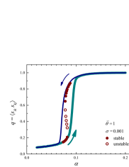
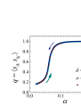
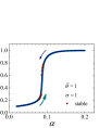
Figure 1: Diagram of $q=\langle s_{ik}s_{kj}\rangle$ vs. $\alpha$ for (a) $\bar{\theta}=1$ , (b) $\bar{\theta}=0.54$ and (c) $\bar{\theta}=1$. In (a) and (b) graphs, $\sigma=0.001$, while in (c) $\sigma=1$ and the network includes $50$ nodes. The solid thin/thick curves show the results of the simulation while the solid/empty circles represent the analytic results. In the simulation, to make it easier to get to the ground state, the value of $\alpha$ was first increased, then reduced from the final value to return to its initial value (follow the arrows, $\stackrel{{\scriptstyle{\color[rgb]{0,0,0.5}\leftarrow}}}{{{\color[rgb]{0.0,0.55,0.55}\boldsymbol{\rightarrow}}}}$). The solid circles ($\bullet$) represent the stable solution while the empty circles ($\boldsymbol{\circ}$) denote the unstable solution that the latter has not appeared in the simulation results.

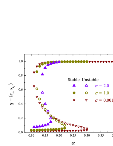
Figure 2: Solid symbols show the stable analytical results for the average of two-star $q$ vs. the coefficient $\alpha$ for the fixed value of $\bar{\theta}=2$ and different values of $\sigma$, while the empty symbols indicate the unstable solutions.

Fig. 2 is a confirmation for the noticeable role of the variance on the hysteresis loop. It depicts the order parameter, $q$, for $\bar{\theta}=2$ and different values of $\sigma$. It displays for a fixed value of the $\bar{\theta}$ by changing the variance the unstable answers deforms. For a range of $\alpha$, where the unstable solution occupies a wider area, reflects the resistance of the system against changes by remembering its past. It takes a while for the system to make the transition. By applying the larger $\sigma$, we induce more heterogeneity therefore the resistance of the system decreases and the unstable answers grab a narrower area hence the hysteresis loop gets smaller.

Fig. 3, indicates the phase diagram of the system. In the coexistence region, $CR$, (shaded area) the self-consistence equation (8) has three solutions corresponds to a symmetric broken phase. In approval of what Newman stated in Ref Park and Newman (2005) there is a critical point, $CP$, separating the coexistence region from high symmetry and low symmetry region. Fig. 3 demonstrates the effect of the variance on the area of the shaded region and where its lowest point is the critical point. Notice that inducing more heterogeneity in the network makes the coexistence region narrower and change the position of the critical point below which the system makes a transition to second order phase transition phenomenologically Park and Newman (2005).

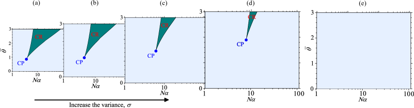
Figure 3: The phase diagram in (N$\alpha$, $\bar{\theta}$) space. For figure a-e the variance of the Gaussian probability distribution of individual benefit is as $0.001,1,2,3,10$ respectively. The dark shaded area corresponds to the coexistence region $(CR)$ in which the system can be in either of two stable states within a hysteresis loop, one of high density (for large value of $\alpha$) and one of low density of triangles (for small value of $\alpha$). Increasing the variance which is equal to inducing more heterogeneity in the network result in shifting the critical point $(CP)$ and the smaller coexistence region.

V Conclusion

Our relationships dictate that each person has an individual identity in addition to a social one and the individual benefit also plays a crucial role in the dynamics of social relationships. For this purpose complex networks represent explanatory models that illustrate us a general picture and lead us in direction of studying real social network. In many studies, the focus was more on global benefit, while in the Strauss model, the individual benefit was given importance along with global ones. Here we made a modification to the Strauss’model by taking into account the heterogeneity of local benefits. Results show:

• The system experiences a first-order phase transition and the hysteresis loop is an indicator that shows the system remembers its past.

• The existence of the hysteresis loop depends on unstable solutions and increasing the variance of the Gaussian probability distribution of links equals heterogeneity in local benefits result in deformation of coexistence region and the width of the hysteresis loop gets narrower.

• The phase diagram indicates that for a small value of $\alpha$ system is in low density of triangles state and by increasing value of $\alpha$ more triads forms and the system is in a condensed state of triangles.

• The location of the critical point ($CP$) in the phase diagram, depends on the mean and the variance of the Gaussian probability distribution of induced heterogeneity and it is increasing by inducing more heterogeneity in the network.

References

- Heider (1946) F. Heider, The Journal of Psychology 21, 107 (1946), pMID: 21010780.
- Heider (2013) F. Heider, The psychology of interpersonal relations (Psychology Press, 2013).
- Kułlakowski et al. (2005) K. Kułlakowski, P. Gawroński, and P. Gronek, International Journal of Modern Physics C 16, 707–716 (2005).
- Cartwright and Harary (1956) D. Cartwright and F. Harary, Psychological Review 63, 277 (1956).
- Albert and Barabási (2002) R. Albert and A.-L. Barabási, Reviews of Modern Physics 74, 47–97 (2002).
- Dorogovtsev and Mendes (2002) S. N. Dorogovtsev and J. F. F. Mendes, Advances in Physics 51, 1079–1187 (2002).
- Newman (2003a) M. E. J. Newman, SIAM Review 45, 167–256 (2003a).
- Newman et al. (2002) M. E. Newman, D. J. Watts, and S. H. Strogatz, Proc. Natl. Acad. Sci. 99, 2566 (2002).
- Jin et al. (2001) E. M. Jin, M. Girvan, and M. E. Newman, Phys. Rev. E 64, 046132 (2001).
- (10) T. Pham, A. Alexander, J. Korbel, R. Hanel, and S. Thurner, Sci. Rep. 11, 17188.
- Minh Pham et al. (2020) T. Minh Pham, I. Kondor, R. Hanel, and S. Thurner, Journal of the Royal Society Interface 17, 20200752 (2020).
- Manshour and Montakhab (2021) P. Manshour and A. Montakhab, Phys. Rev. E 104, 034303 (2021).
- Shojaei et al. (2019) R. Shojaei, P. Manshour, and A. Montakhab, Phys. Rev. E 100, 022303 (2019).
- Leik and Meeker (1975) R. Leik and B. Meeker, Mathematical Sociology, Prentice-Hall methods of social sciences series (Prentice-Hall, 1975).
- Saiz et al. (2017) H. Saiz, J. Gómez-Gardeñes, P. Nuche, A. Girón, Y. Pueyo, and C. L. Alados, Ecography 40, 733 (2017).
- Moradimanesh et al. (2021) Z. Moradimanesh, R. Khosrowabadi, M. E. Gordji, and G. Jafari, Sci. Rep. 11, 1 (2021).
- Rizi et al. (2021) A. K. Rizi, M. Zamani, A. Shirazi, G. R. Jafari, and J. Kertész, Frontiers in Physiology 11, 1792 (2021).
- Rabbani et al. (2019) F. Rabbani, A. H. Shirazi, and G. R. Jafari, Phys. Rev. E 99, 062302 (2019).
- Bagherikalhor et al. (2021) M. Bagherikalhor, A. Kargaran, A. H. Shirazi, and G. R. Jafari, Phys. Rev. E 103, 032305 (2021).
- Masoumi et al. (2021) R. Masoumi, F. Oloomi, A. Kargaran, A. Hosseiny, and G. R. Jafari, Phys. Rev. E 103, 052301 (2021).
- Kargaran et al. (2020) A. Kargaran, M. Ebrahimi, M. Riazi, A. Hosseiny, and G. R. Jafari, Phys. Rev. E 102, 012310 (2020).
- Watts and Strogatz (1998) D. J. Watts and S. H. Strogatz, Nature 393, 440 (1998).
- Caldarelli et al. (2004) G. Caldarelli, R. Pastor-Satorras, and A. Vespignani, The European Physical Journal B 38, 183 (2004).
- Newman (2003b) M. E. Newman, Phys. Rev. E 68, 026121 (2003b).
- Holme and Kim (2002) P. Holme and B. J. Kim, Phys. Rev. E 65, 026107 (2002).
- Strauss (1986) D. Strauss, SIAM Review 28, 513 (1986).
- Burda et al. (2004a) Z. Burda, J. Jurkiewicz, and A. Krzywicki, Phys. Rev. E 69, 026106 (2004a).
- Burda et al. (2004b) Z. Burda, J. Jurkiewicz, and A. Krzywicki, Phys. Rev. E 70, 026106 (2004b).
- Park and Newman (2005) J. Park and M. E. Newman, Phys. Rev. E 72, 026136 (2005).
- Yook et al. (2001) S. H. Yook, H. Jeong, A.-L. Barabási, and Y. Tu, Phys. Rev. Lett. 86, 5835 (2001).
- Noh and Rieger (2002) J. D. Noh and H. Rieger, Phys. Rev. E 66, 066127 (2002).
- Barrat et al. (2004a) A. Barrat, M. Barthelemy, R. Pastor-Satorras, and A. Vespignani, Proc. Natl. Acad. Sci. 101, 3747 (2004a).
- Barrat et al. (2004b) A. Barrat, M. Barthélemy, and A. Vespignani, Phys. Rev. Lett. 92, 228701 (2004b).
- Frank and Strauss (1986) O. Frank and D. Strauss, Journal of the American Statistical Association 81, 832 (1986).
- Billard (2005) L. Billard, Journal of The A merican Statistical Association, Vol. 4 (Wiley Online Library, 2005).
- Snijders et al. (2006) T. A. Snijders, P. E. Pattison, G. L. Robins, and M. S. Handcock, Sociological Methodology 36, 99 (2006).
- Snijders (2011) T. A. Snijders, Annual Review of Sociology 37, 131 (2011).
- Park and Newman (2004a) J. Park and M. E. Newman, Phys. Rev. E 70, 066146 (2004a).
- Park and Newman (2004b) J. Park and M. E. Newman, Phys. Rev. E 70, 066117 (2004b).
- Antal et al. (2005) T. Antal, P. L. Krapivsky, and S. Redner, Phys. Rev. E 72, 036121 (2005).