Empirical LiK excited state potentials: connecting short range and near dissociation expansions
	Sofia Botsi,a Anbang Yang,a Mark M. Lam,a Sambit B. Pal,a Sunil Kumar,a Markus Debatin,a and Kai Dieckmann∗a,b
	We report on a high-resolution spectroscopic survey of ${}^{6}\textrm{Li}{}^{40}\textrm{K}$ molecules near the $2\textrm{S}+4\textrm{P}$ dissociation threshold and produce a fully empirical representation for the $\textrm{B}^{1}\Pi$ potential by connecting available short- and long-range data. The purpose is to identify a suitable intermediate state for a coherent Raman transfer to the absolute ground state, and the creation of a molecular gas with dipolar interactions. Starting from weakly bound ultracold Feshbach molecules, the transition frequencies to twenty-six vibrational states are determined. Our data are combined with long-range measurements [Ridinger et al., EPL, 2011, 96, 33001], and near-dissociation expansions for the spin-orbit coupled potentials are fitted to extract the $C_{6}$ dispersion coefficients. A suitable vibrational level is identified by resolving its Zeeman structure and by comparing the experimentally attained g-factor to our theoretical prediction. Using mass-scaling of the short-range data for the $\textrm{B}^{1}\Pi$ [Pashov et al., Chem. Phys. Lett., 1998, 292, 615-620] and an updated value for its depth, we model the short- and the long-range data simultaneously and produce a Rydberg-Klein-Rees curve covering the entire range.

1 Introduction

Ultracold dipolar molecules have long been in the focus of experimental and theoretical research due to their long-range and anisotropic interaction ^{1, 2, 3}. They provide a highly sensitive and robust platform for exploring the areas of quantum information processing ^{4, 5, 6, 7} and quantum simulation of long-range spin models ^{8, 9, 10}. They may as well play a significant role in precision measurements ^{11, 12, 13}, research on ultracold chemistry ^{14, 15, 16} and as recently proposed in probing new physics beyond the Standard Model ^{17, 18}. Their rich internal structure and molecular complexity however, renders their creation and coherent control a challenge. Thus far, a variety of bi-alkali dimers have been produced in their absolute singlet ro-vibronic ground state ^{19, 20, 21, 22, 23, 24, 25} by utlizing the coherent transfer scheme of stimulated Raman adiabatic passage (STIRAP) ²⁶, in which the high initial molecular phase-space density is preserved. The remarkable achievement of molecular quantum degeneracy has been achieved only for the case of ${}^{40}\textrm{K}{}^{87}\textrm{Rb}$ ²⁷. Alternative production approaches include direct laser cooling of the sample from a buffer gas source ²⁸, and individual control of heavy neutral molecules in optical tweezers ^{29, 30}. Regarding the traditional three-level STIRAP scheme, obtaining the desired efficient ground state transfer necessitates a detailed understanding of the molecular structure and an extensive spectroscopic survey for the identification of a suitable electronically excited state ^{31, 32, 33}. Selection rules for electronic transitions, Franck-Condon overlap factors, mixing mechanisms between intermediate states and tuning capabilities of the available resources, are amongst some of the factors that need to be considered for making such a selection.

In this paper, we present results from the spectroscopic investigation of such intermediate candidate states, which is motivated by the objective to transfer ${}^{6}\textrm{Li}{}^{40}\textrm{K}$ molecules to the ground state. The long-range part of the low-lying $\textrm{B}^{1}\Pi$ was discussed in our previous work ³⁴ as a possible candidate, and a specific vibrational sub-level was selected. Here, we show the long-range spectrum below the ⁶Li($2^{2}$S_1/2)+⁴⁰K($4^{2}$P_3/2) asymptote and the line assignment analysis. In order to understand the spectral structure, we explore the intermediate state mixing due to the spin-orbit coupling interaction. The Zeeman sub-structure of the selected vibrational level is resolved and the experimentally attained g-factor is compared to our theoretical prediction. To access the levels of the $\textrm{B}^{1}\Pi$ potential, we associate ultracold ${}^{6}\textrm{Li}$ and ${}^{40}\textrm{K}$ atoms via a magnetically tunable Feshbach resonance ³⁵ and apply spectroscopic light. This scheme differs from previous studies, which were performed by conventional photoassociation (PA) in a dual-species magneto-optical trap (MOT) ³⁶ and by Doppler-free polarization labelling spectroscopy (PLS) of the ${}^{7}\textrm{Li}{}^{39}\textrm{K}$ isotopologue in a heat-pipe ³⁷. They provide important information on a wide range of the excited spectrum, but they do not cover all the levels in the region of our interest. The PA results when combined with our data, apart from facilitating the level assignment, assist in inferring the $C_{6}$ parameters. By combining them with the PLS observations, we produce a complete empirical Rydberg-Klein-Rees (RKR) ^{38, 39, 40} curve for the $\textrm{B}^{1}\Pi$ potential.

2 Spectroscopic results and line assignment

The starting point of our experiments is the creation of a quantum degenerate mixture of $10^{5}$ ${}^{6}\textrm{Li}$ and $8\times 10^{4}$ ${}^{40}\textrm{K}$ atoms in a magnetic trap, which is sympathetically cooled via evaporative cooling of bosonic ${}^{87}\textrm{Rb}$ ⁴¹. The Fermi-Fermi mixture is then transferred into a crossed optical dipole trap, where ${}^{6}\textrm{Li}$ and ${}^{40}\textrm{K}$ atoms are prepared in the $\ket{F_{\mathrm{Li}}=1/2,m_{F,\mathrm{Li}}=-1/2}$ and $\ket{F_{\mathrm{K}}=9/2,m_{F,\mathrm{K}}=-9/2}$ hyperfine states. Here, $F$ is the hyperfine quantum number and $m_{F}$ its respective projection along the internuclear axis. Magneto-association is performed by sweeping the magnetic field across an interspecies Feshbach resonance located at $21.56\,$mT, which results in up to $10^{4}$ Feshbach molecules ⁴². The molecular state contains a significant admixture from the singlet ground state potential ⁴³ and is an excellent starting point for the excited state spectroscopy. Uncombined free atoms are spatially separated from weakly bound molecules by means of an inhomogeneous magnetic-field pulse, as the latter possess an almost vanishing magnetic moment. The pulse is applied during time-of-flight (TOF) after release from the trap, and is followed by detection via absorption imaging.

The ultracold mixture is illuminated by spectroscopic light and one-photon spectroscopy is performed for the investigation of the vibrational levels of the excited potentials during TOF before imaging. If the spectroscopic light is resonant with an electronically excited state, then the molecules undergo resonant excitation and subsequent spontaneous decay, which is highly likely to occur to some other molecular bound state of the ground state and not to the initial Feshbach state. This process will manifest as a loss in the number of detected molecules during absorption imaging of the Feshbach state. Since this scheme is destructive, a new molecular sample is prepared after each experimental cycle. The spectroscopic source is a commercial external cavity diode laser (Toptica DL Pro), which is tunable over a broad wavelength range of $760\,$nm to $775\,$nm and has a nominal output power of $28\,$mW. The laser’s frequency is measured by an optical beat note with a frequency comb (FC) that is deriving its long-term stability from a GPS-disciplined RF reference generator. To determine the frequency of the laser to within one free spectral range of the FC, a home-built wavemeter is utilized. It has an accuracy of $10\,$MHz, which is accomplished by referencing it to a laser locked to the potassium D2-line.

Table 1:  Measured long-range vibrational levels close to the 2S+4P asymptote. Counting is downwards from the dissociation threshold. The transition frequencies are computed with respect to the hyperfine free ground state asymptote. The frequency detunings utilized for obtaining the $C_{6}$ coefficients are referenced to the same hyperfine state of the excited state asymptote as the one used in ⁴⁴

state	group	$v$	f${}_{\textrm{laser}}$ (THz)	$\Delta$f (GHz)
$\Omega$=1${}^{\textrm{up}}$	dyad	-6	390.474969	544.52
		-7	390.154969	864.52
		-8	389.734896	1284.32
		-9	389.215496	1803.72
		-10	388.611196	2408.02
		-11	387.925196	3094.02
		-12	387.125196	3894.02
$\Omega$=0${}^{\textrm{+}}$	upper triad	-7	390.606196	413.02
		-8	390.396196	623.02
		-9	390.129196	890.02
		-10	389.781196	1238.02
		-11	389.347196	1672.02
		-12	388.865196	2154.02
$\Omega$=0${}^{\textrm{-}}$	upper triad	-7	390.577196	442.02
		-8	390.356196	663.02
		-9	390.082196	937.02
		-10	389.737196	1282.02
		-11	389.337196	1682.02
$\Omega$=1${}^{\textrm{down}}$	upper triad	-7	390.521196	498.02
$\Omega$=0${}^{\textrm{+}}$	lower triad	-4	389.171196	118.52
		-5	389.037196	251.90
		-6	388.855196	433.90
		-7	388.621196	667.90
$\Omega$=1	lower triad	-3	389.215496	73.60
		-4	389.109961	179.90
		-5	388.925196	363.90

In Table 1 we present a summary of the measured long-range states located up to $4\,$THz below the ⁶Li($2^{2}$S_1/2)+⁴⁰K($4^{2}$P_3/2) asymptote. To enable a broad survey, the spectroscopic resolution of the measurement is initially set to $1\,$GHz. This is sufficient to unambiguously identify the states, since the level spacing between adjacent vibrational levels is much larger. The experimentally observed transitions are assigned to the nearest predicted level based on extrapolation of the PA lines, for which the assignment was done based on progressions described by the LeRoy-Bernstein law ³⁶ as further described in Section 4. Six vibrational series are distinguished from each other which contain a total of $26$ vibrational levels. The long-range potentials are coupled by the strong spin-orbit interaction and are labelled with the quantum number $\Omega^{\pm}$, as is suitable for Hund’s case (c) molecules. $\Omega$ is the projection of the coupled angular momentum $\textbf{J}_{a}=\textbf{S}+\textbf{L}$ on the molecular axis, where $S$ is the total spin and $L$ is the orbital angular momentum. The $\pm$ denotes the reflection symmetry of the spatial component of the electronic wave function through a plane containing the internuclear axis and the superscripts up/down further classify the long-range states into groups of potentials for unambiguous distinction. The frequency detunings are computed by subtracting from our measured transition frequencies the energy of the Feshbach molecular state with respect to the hyperfine-free ground state asymptote ⁶Li($2^{2}$S_1/2)+⁴⁰K($4^{2}$P_3/2). This energy contains the binding

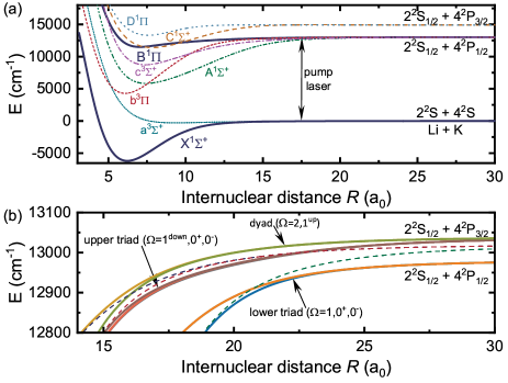
Fig.  1: Potential energy curves of ${}^{6}\textrm{Li}{}^{40}\textrm{K}$ molecules. (a) Adiabatic potentials, with no spin-orbit coupling effects considered, connecting to the lowest three electronic asymptotes. The ground state potential is given by Tiemann et al. ⁴⁵ and the excited state potentials by Allouche ⁴⁶. (b) Spin-orbit coupled potentials near the dissociation threshold. The dyad ($\Omega=2,1^{\textrm{up}}$), upper triad ($\Omega=0^{+},0^{-},1^{\textrm{down}}$) and lower triad ($\Omega=1,0^{+},0^{-}$) are labelled. Bare potentials are included with dashed lines to show the rapidly diminishing perturbation caused by the spin-orbit coupling as deeper bound levels are considered

energy of the molecular state and its Zeeman shift at the Feshbach magnetic field of $21.56\,$mT ($472.5\,$MHz), and the atomic hyperfine energies of ${}^{6}\textrm{Li}$ ($152.1\,$MHz) and ${}^{40}\textrm{K}$ ($571.5\,$MHz) for the respective asymptotic states.

Further characterization of the long-range states requires a detailed study of the spin-orbit coupling interaction, which leads to the mixing of neighboring singlet and triplet potentials and becomes dominant at large internuclear distances. Here, the relevant excited short-range curves which result into the coupled long-range potentials are the $\textrm{B}^{1}\Pi$, $\textrm{b}^{3}\Pi$, $\textrm{A}^{1}\Sigma^{+}$ and the $\textrm{c}^{3}\Sigma^{+}$ as shown in Fig. 1(a), where the $\textrm{A}^{1}\Sigma^{+}$ and $\textrm{b}^{3}\Pi$ cross at an internuclear distance of $7.5\,\textrm{a}_{0}$, as is commonly observed in alkali dimers. Fig. 1(b) shows the region of strongest spin-orbit coupling, where the eight Hund’s case (c) long-range states dissociate to both of the $2\textrm{S}+4\textrm{P}$ asymptotes of the ${}^{6}\textrm{Li}{}^{40}\textrm{K}$ molecule. The singlet-triplet mixing is calculated by projecting the spin-orbit coupled states onto the bare potential basis. This is necessary to facilitate the selection of a suitable intermediate state that will mediate coupling between the dominantly singlet Feshbach molecular state and the singlet ground state for the two-photon transfer. The $\Omega=1^{\textrm{up}}$ state of the dyad and the $\Omega=0^{-}$ state of the upper triad meet this requirement, as they contain a large singlet component and connect to singlet bare potentials in the short-range (Fig. S1). Moreover, the $\Delta\Omega=0,\pm 1$ and $\Delta S=0$ selection rules further narrow down the choice, making the $\Omega=1^{\textrm{up}}$ potential a promising option.

3 Zeeman effect for Hund’s case (c) molecules

To identify the $\Omega$=1${}^{\textrm{up}}$ state as a suitable intermediate state, it is desirable to resolve its characteristic magnetic Zeeman structure. Here, only the rotational ground state is of interest, and therefore the total angular momentum is $J=1$. Three magnetic sublevels are expected, which are denoted by $M_{J}$. For this measurement scans with higher resolution are performed by employing an interferometric frequency stabilization device, which provides in-lock frequency tuning of the laser in MHz steps over a large range ⁴⁷. In order to resolve the magnetic sub-structure, we iteratively adjust the spectroscopy laser power to avoid power-broadening and reduce the irradiation time. In Fig. 2 the Zeeman triplet substructure of the $v=-11$ vibrational level is shown, where $v$ is the vibrational quantum number. It is measured at two different magnetic fields, specifically at the $15.54\,$mT and at the $21.56\,$mT Feshbach resonance of ${}^{6}\textrm{Li}{}^{40}\textrm{K}$. Zeeman splittings of $122\,$MHz and $185\,$MHz are observed, respectively. This is consistent with a linear Zeeman effect and an average g-factor of $g_{\textrm{exp.}}=0.59$. In the following, this value is compared to the theoretical prediction for the g-factor for the Hund’s case (c) vector coupling scheme, where we generally represent the vibrational levels in the coupled $\ket{v(\Omega),J_{a};\Omega,\epsilon,J,M_{J}}$ basis. Here, the total parity $\epsilon$ is specified, which is related to whether symmetric or anti-symmetric combinations of $\pm\Omega$-states are utilized. The effective Hamiltonian describing the interaction between the external magnetic field and electron spin and the orbital magnetic moments in spherical tensor notation is ⁴⁸:

$$\mathcal{H}_{Z}=g_{s}\mu_{\textrm{B}}\textrm{T}^{1}(\textbf{B})\cdot\textrm{T}^{1}(\textbf{S})+g_{L}\mu_{\textrm{B}}\textrm{T}^{1}(\textbf{B})\cdot\textrm{T}^{1}(\textbf{L})\quad,$$ (1)

where $\mu_{\textrm{B}}$ is the Bohr magneton and $g_{S}$ and $g_{L}$ are the g-factors for the electron spin and the orbital motion respectively. The effective g-factor is then directly related to the expectation value via $\left<\mathcal{H}_{Z}\right>=M_{J}g_{\textrm{(c)}}\mu_{\textrm{B}}B$. In order to evaluate $\left<\mathcal{H}_{Z}\right>$, we follow the general scheme as exemplified in ⁴⁹ that expands to the reduced matrix elements that can be evaluated with the help of the quantum numbers of the uncoupled basis. As the observed Zeeman shift is smaller than the rotational constants of the $v=-11$, off-diagonal matrix element for different $J$ do not need to be considered. Then, for our case of rotationless excitation to the $\Omega=1^{\textrm{up}}$ state, we have $J_{a}=1$ and the Zeeman shift is the same for both parity eigenstates. As we work with the $2\textrm{S}+4\textrm{P}$ asymptote, $L=1$ is the sole contribution to the spin-orbit coupled state. However, for the spin, the superposition of the $S=0$ and $S=1$ states contributing to the $\Omega=1^{\textrm{up}}$ state needs to be considered. From our analysis of the spin-orbit coupling (Fig. S1), we see that for the long-range there is an equal admixture of the $\ket{{}^{1}\Pi}$ and $\ket{{}^{3}\Pi}$ components, whereas for the short-range the state becomes purely of $\ket{{}^{1}\Pi}$ character. Hence, we adopt a simple approach by taking the average of the results for the g-factor between the short-range and long-range spin compositions. A more accurate calculation would require to integrate the spin composition weighted by the probability density of the corresponding vibrational wave function. Here, we find as a result a g-factor for the $\Omega$=1${}^{\textrm{up}}$ state of $g_{\textrm{(c)}}=0.625$, which is in good agreement with the measured value.

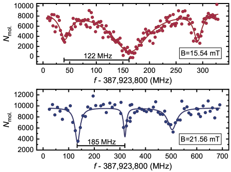
Fig.  2: Zeeman triplets for the $v=-11$ level measured at two different magnetic fields. The relative size of Zeeman components changes with polarization. The Zeeman splittings correspond to a measured average g-factor value, which is in good agreement with our theoretical prediction

In comparison, for the Hund’s case (a) the respective value is $g_{\textrm{(a)}}=(\Lambda+2\Sigma)\Omega/J(J+1)=0.5$ ⁵⁰, where $\Lambda$ is the projection of L along the intermolecular axis. Therefore, the measurements of the Zeeman effect support the validity of the Hund’s case (c) coupling scheme as an appropriate description for vibrational levels as deeply bound as the $v=-11$.

4 Near-dissociation expansions and $C_{6}$ coefficients

To achieve a more complete characterization of the long-range behavior of the potentials, the data set based on PA measurements ³⁶ is extended by our measurements of more deeply bound vibrational levels, as already mentioned in Section 2. This allows to determine the $C_{6}$ dispersion coefficients from a larger data set for each vibrational progression. Additionally, the description by the semi-classical LeRoy-Bernstein formula is extended and near-dissociation expansions (NDE) are used ^{51, 52}.

The PA measurements resulted in seven vibrational series below the ${}^{6}\textrm{Li}(2^{2}$S${}_{1/2})+{}^{40}\textrm{K}(4^{2}$P${}_{3/2})$ asymptote. In order to combine our data to the PA measurements, we compute the frequency detunings $\Delta$f (shown in Table 1) with respect to the ${}^{40}\textrm{K}$ $4S_{1/2}(F=9/2)\rightarrow 4P_{3/2}(F^{\prime}=11/2)$ hyperfine transition frequency ⁵³, which is used as a reference for the PA measurements ⁴⁴. For the data comparison we assume the hyperfine-free asymptotic energy of the $\textrm{X}^{1}\Sigma^{+}$ ground state as a reference point for our measurements. This reflects that the PA measurements were performed in a MOT, where for the initial states all four hyperfine ground states of ${}^{6}\textrm{Li}$ and ${}^{40}\textrm{K}$ are possible. Hence, the resulting frequency uncertainty in the data comparison is on the order of the hyperfine energies, which is comparable to the measurement resolution of $1\,$GHz. A more precise comparison would require hyperfine resolved measurements, which are difficult to be achieved for all the PA lines.

The general NDE expressions for the vibrational energies $G_{v}$ and the rotational constants $B_{v}$ are ^{54, 55}:

$$G_{v}=\mathcal{D}-K_{0}^{\infty}(v)\crossproduct\mathcal{F}_{0}(v_{\mathcal{D}}-v)$$ (2)

$$B_{v}=K_{1}^{\infty}(v)\crossproduct\mathcal{F}_{1}(v_{\mathcal{D}}-v)\quad,$$

where $\nu_{\mathcal{D}}$ is the extrapolated non-integer effective vibrational index at the dissociation energy $\mathcal{D}$. The $K_{m}^{\infty}(v)$ functions are:

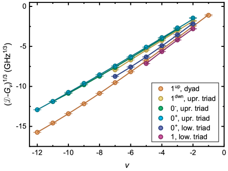
Fig.  3: Cubic root of the binding energies plotted for various vibrational levels of the long-range potentials by combining our data with the PA measurements. The states belonging to the upper- and the lower triad are grouped together since they dissociate to the same asymptote

$$K_{m}^{\infty}(v)=X_{m}(n,C_{n},\mu)(v_{\mathcal{D}}-v)^{[2n/(n-2)]-2m}\quad,$$ (3)

where $X_{m}(n,C_{n},\mu)=\bar{X}_{m}(n)/[\mu^{n}C_{n}^{2}]^{1/n-2}$ are numerical factors depending on physical constants ⁵⁶ and $\mu$ is the Watson’s charge-modified reduced mass. The empirically determined functions $\mathcal{F}_{m}(v_{\mathcal{D}}-v)$ that are required to approach unity close to the dissociation threshold are expressed in the form of a Padé expansion using rational polynomials ⁵⁷:

Table 2:  Values of the $C_{6}$, $v_{\mathcal{D}}$ and $p_{2}^{0}$ fitting parameters and their respective errors $\delta C_{6}$, $\delta$v_D and $\delta p_{2}^{0}$ as obtained from fitting to a NDE with $S=1$. The expansion to which the parameters apply is given in parentheses. The values of the $p_{2}^{0}$ parameters are multiplied by $10^{2}$. The $C_{6}$ parameters are given in atomic units

$\Omega$	$C_{6}$ $\pm$ $\delta C_{6}$	$v_{\mathcal{D}}$ $\pm$ $\delta v_{\mathcal{D}}$	$p_{2}^{0}\pm\delta p_{2}^{0}$	$p_{2}^{0}\pm\delta p_{2}^{0}$
	($G_{v},B_{v}$)	($G_{v},B_{v}$)	($G_{v}$)	($B_{v}$)
1${}^{\textrm{up}}$	8619 $\pm$ 736	-0.29 $\pm$ 0.07	-0.16 $\pm$ 0.02	0.16 $\pm$ 0.72
0${}^{\textrm{+}}$	30391 $\pm$ 4984	-0.65 $\pm$ 0.13	-0.08 $\pm$ 0.04	1.35 $\pm$ 1.01
0${}^{\textrm{-}}$	24880 $\pm$ 3016	-0.65 $\pm$ 0.10	-0.16 $\pm$ 0.03	0.43 $\pm$ 0.88
1${}^{\textrm{down}}$	27717 $\pm$ 8474	-0.46 $\pm$ 0.16	0.08 $\pm$ 0.22	0.81 $\pm$ 0.73
0${}^{\textrm{+}}$	8251 $\pm$ 2169	-0.55 $\pm$ 0.13	-0.50 $\pm$ 0.18	6.68 $\pm$ 5.02
1	13309 $\pm$ 9098	0.05 $\pm$ 0.24	0.54 $\pm$ 0.89

$$\mathcal{F}_{m}(v_{\mathcal{D}}-v)=\Bigg{(}\frac{1+\sum_{i=t}^{L}p_{i}^{m}(v_{\mathcal{D}}-v)^{i}}{1+\sum_{j=t}^{M}q_{j}^{m}(v_{\mathcal{D}}-v)^{j}}\Bigg{)}^{S}\quad,$$ (4)

where the power of the exponent $S$ is set at either $S=1$ to yield an ”outer” expansion, or at $S=2n/(n-2)$, to yield an ”inner” expansion. The $p_{i}^{m}$ and $q_{j}^{m}$ are the parameters of the expansion. For the case of the leading terms of the attractive long-range potentials having powers of $n=6$ or $n=8$, $t=1$ is applicable ⁵⁸.

The measured lines are shown in Fig. 3, where the cubic root of the vibrational energies relative to the excited state asymptote is plotted versus the vibrational index $v$ for the extended data set. For each long-range potential, the $C_{6}$ coefficients, the $v_{\mathcal{D}}$ values, as well as the expansion parameters are extracted from the fitting and are listed in Table 2 along with their error estimates. An ”outer” expansion is performed for all of the $\Omega$ states. Various combinations of the $p_{i}^{m}$ and $q_{j}^{m}$ expansion parameters extended to different orders are tested for each long-range potential and the fitting quality is assessed. To avoid large estimation errors due to a large number of fitting parameters, a second order expansion using only $p_{2}^{0}$ is performed for all the excited states. It should be noted here that this Padé analysis directly corresponds to using the improved LeRoy-Bernstein NDE formula ⁵⁹ for the case of $n=6$. The latter makes use of a quadratic term as the leading order beyond the pure $C_{6}$ semiclassical LeRoy-Bernstein formula.

Most of our extracted $C_{6}$ values agree within 10% with the PA results and the respective theoretical predictions ⁶⁰. A slightly higher deviation is observed for the $\Omega$=1${}^{\textrm{up}}$. For this state the modified LeRoy-Bernstein radius ⁶¹ is $R_{\textrm{mLR}}=19.8\,$a₀, while the deepest bound vibrational level reached by our measurements possesses a classical outer turning point at $15.6\,$a₀, as inferred from the RKR analysis presented in the next section. Similarly for the $\Omega$=0${}^{\textrm{+}}$ state of the lower triad $R_{\textrm{mLR}}=29.5\,$a₀, while the deepest measured vibrational level has its turning point at $20.8\,$a₀. Nevertheless, we observe that the $C_{6}$ values remain stable, when varying the extend of the data set to include only less deeply bound vibrational levels. In contrast, when a pure $C_{6}$ expansion is utilized, the resulting dispersion coefficient varies strongly with the extend of the used data set. Hence, a NDE method is clearly more appropriate than a pure $C_{6}$ semiclassical LeRoy-Bernstein formula. For the two long-range states belonging to the lower triad, the contribution of the next higher order $C_{8}/R^{8}$ term in the multipolar expansion of the interaction potential needs to be considered. At intermolecular distances of $64.4\,$a₀ and $50.7\,$a₀ for the $\Omega$=0${}^{\textrm{+}}$ and the $\Omega$=1 state respectively, which are well within our spectroscopic reach, the contributions of the $C_{8}$ coefficients become significant and need to be included in the NDE formula. However, it has been suggested ^{32, 62} that the precise value of the C₈ is hard to obtain accurately when fitting with the improved LeRoy-Bernstein NDE expression. Due to the limited number of measured lines for these states, accurate modeling with a NDE including a larger number of fitting parameters is not feasible.

In the short-range a large data basis is available for rotationally excited states from the PLS measurements. For the purpose of extending the description of rotationally excited states to the long-range, a NDE for the rotational energies $B_{v}$ is fitted with the respective expression introduced in eqn (2). However, for this purpose only a small data set from the PA measurements is available, since our spectroscopy does not cover rotationally excited states. A Padé expansion with one $p_{2}^{0}$ parameter is utilized, where the $C_{6}$ and $v_{\mathcal{D}}$ parameters are taken from our $G_{v}$ fits. The results are included in Table 2.

5 Combining short- and long-range data

Thus far, merging our measurements with the PA observations yields an extended characterization of the spin-orbit coupled states near the threshold. This holds in particular for the $\Omega$=1${}^{\textrm{up}}$, which is of interest as an intermediate state for the two-photon transfer of the Feshbach molecules to the dipolar ground state. This state connects to the $\textrm{B}^{1}\Pi$ potential in the short-range (Fig. S1). At the inner turning point high-lying vibrational levels of this potential have a large Franck-Condon overlap with the absolute ground state, favoring large transitions strengths. For the $\textrm{B}^{1}\Pi$ potential a large data set exists in the short-range for the ${}^{7}\textrm{Li}{}^{39}\textrm{K}$ isotopologue measured by PLS ³⁷. Here, we combine the short-range and long-range data to attain an improved potential curve. To our knowledge it is unique that an excited potential is supported by empirical data throughout almost the entire internuclear range. The short-range data cover the range from the $v=-33$ vibrational ground state up to the $v=-15$ level. Our measurements cover the $v=-12$ to $v=-6$ states, whereas the PA data range from $v=-5$ to the $v=-1$. From our analysis it is apparent that there are no available experimental results for the $v=-14$ and $v=-13$ levels.

To facilitate the combination of the data we use mass-scaling of the Dunham coefficients determined by the PLS measurements to our ${}^{6}\textrm{Li}{}^{40}\textrm{K}$ isotopologue by the ratio of the reduced masses $\widetilde{\mu}=\mu\left({}^{7}\textrm{Li}{}^{39}\textrm{K}\right)/\mu\left({}^{6}\textrm{Li}{}^{40}\textrm{K}\right)$. The vibrational term energies obtained from the Dunham expansion are:

$$T(\tilde{v},J)=T_{\mathrm{e}}({\textrm{B}^{1}\Pi})+\sum_{k,l}\widetilde{\mu}^{(l+k)/2}Y_{k,l}(\tilde{v}+\frac{1}{2})^{k}(J(J+1))^{l}\quad,$$ (5)

where $Y_{k,l}$ are the Dunham coefficients, $\tilde{v}$ is the vibrational level indexed by positive numbers starting from $\tilde{v}=0$ for the ground state. As the PLS data are obtained by measuring transitions originating from low-lying states of the $\textrm{X}^{1}\Sigma^{+}$, the term energy for the excited state potential $T_{\mathrm{e}}({\textrm{B}^{1}\Pi})$ is defined relative to the minimum of the ground state potential ³⁷. In the same work the short-range data are extrapolated to obtain the asymptotic energy of the $\textrm{B}^{1}\Pi$ potential and hence infer the potential depth $\mathcal{D}({\textrm{B}^{1}\Pi})$. Here, we calculate the depth in a different way to combine the short-range data with the long-range data, both referenced to the $\textrm{B}^{1}\Pi$ asymptote. From our previous high-resolution two-photon spectroscopy of the $\textrm{X}^{1}\Sigma^{+}$ ground state ⁴³ the depth of the ground state potential was accurately measured as $\mathcal{D}(\textrm{X}^{1}\Sigma^{+})=6216.863166\,$cm^-1. Further, the wavenumber of the D2-potassium atomic transition $\bar{\lambda}_{\mathrm{D2}}=13042.899700\,$cm^-1 is known from literature ⁵³. Therefore, an improved value for the depth of the excited state potential can be inferred from the measured data as:

$$\mathcal{D}({\textrm{B}^{1}\Pi})=\mathcal{D}(\textrm{X}^{1}\Sigma^{+})+\bar{\lambda}_{\mathrm{D2}}-T_{\mathrm{e}}({\textrm{B}^{1}\Pi})=1687.002866\,\textrm{cm}^{-1}\quad.$$ (6)

We produce an updated semiclassical RKR potential curve for the ${\textrm{B}^{1}\Pi}$ using the RKR1 program by LeRoy ⁶³. The RKR1 program allows for a mixed representation of the ro-vibrational energies by the mass-scaled Dunham parameters $Y_{k,l}$ for the short-range, and simultaneously by the near-dissociation expansion parameters $C_{6}$, $v_{\mathcal{D}}$ and $p_{2}^{0}$ (vibrational and rotational)

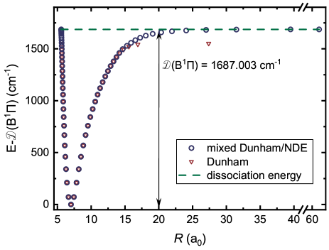
Fig.  4: Complete empirical RKR curve for the excited $\textrm{B}^{1}\Pi$ potential. A mixed Dunham/NDE representation is utilized for the vibrational energies (blue circles). A pure Dunham representation (red triangles) fails to accurately account for the shape of the potential near the outer turning points

for the long-range. We make use of $\mathcal{D}({\textrm{B}^{1}\Pi})$ to relate the two energy scales. The RKR1 program interpolates between the two ranges by utilizing a switching function $F_{\textrm{s}}(v)=\bigl{\{}1+exp\big{(}(v-v_{\textrm{s}})/\delta v_{\textrm{s}}\big{)}\bigr{\}}^{-1}$. We use $v_{\textrm{s}}=-14$ and $\delta v_{\textrm{s}}=0.5$ for the switch-over point and range, which is conveniently located at the small gap of available vibrational experimental data. The resulting RKR potential curve is shown in Fig. 4 represented by the inner and outer classical turning points for each vibrational level. The corresponding numerical values are tabulated in Table S2. For comparison a potential curve only based on the Dunham representation is plotted as well. As seen in Fig. 4, the Dunham curve fails to correctly represent the limiting near-dissociation behavior of the vibrational energies as expected.

6 Conclusions

To conclude, an extensive investigation of the vibrational states of ${}^{6}\textrm{Li}{}^{40}\textrm{K}$ molecules below the ⁶Li($2^{2}$S_1/2)+⁴⁰K($4^{2}$P_3/2) asymptote was presented. Starting from Feshbach molecules, high-resolution one-photon loss spectroscopy of the excited spin-orbit coupled potentials revealed 26 vibrational levels. The combination with published data from photoassociation spectroscopy led to the complete characterization of the long-range part by near-dissociation expansion expressions and improved $C_{6}$ coefficients. In a next step the data were combined with existing mass-scaled data covering the short range of the $\textrm{B}^{1}\Pi$ potential. This allowed for the situation of empirical data covering the complete range of a molecular potential, which to our knowledge is unique for bi-alkali molecules. We additionally determined an updated value for the depth of the ${\textrm{B}^{1}\Pi}$ based on new spectroscopic data of the ground state potential. Hence, a complete empirical RKR potential was computed.

The states of the spin-orbit coupled $\Omega$=1${}^{\textrm{up}}$ potential were investigated in particular, since it is directly connected to the $\textrm{B}^{1}\Pi$ in the short-range. The experimentally resolved Zeeman splitting of the $v=-11$ vibrational sub-level was used to identify the states of the $\Omega$=1${}^{\textrm{up}}$ potential and the experimentally obtained g-factor was found in good agreement with our theoretical prediction for Hund’s case (c). We believe that the characterization of the $\Omega$=1${}^{\textrm{up}}$ states is of particular importance for the purpose of finding a spectroscopic pathway for the transfer of the Feshbach molecules to the absolute ground state and the creation of a dipolar quantum gas. This is as at the inner turning point, the shallow $\textrm{B}^{1}\Pi$ potential offers excellent Franck-Condon overlap with the ground state wave function at accessible wavelengths. As no hyperfine-structure was resolved for the $\Omega$=1${}^{\textrm{up}}$ state in ⁶Li⁴⁰K, a similar approach as discussed in ⁴³ based on addressing a Zeeman component of the excited state by polarized light can be employed to control the hyperfine states for this pathway.

Conflicts of interest

There are no conflicts to declare.

Supplementary Information:
Empirical LiK excited state potentials: connecting short range and near dissociation expansions

Sofia Botsi,^a Anbang Yang,^a Mark M. Lam,^a Sambit B. Pal,^a Sunil Kumar,^a Markus Debatin,^a and Kai Dieckmann^∗a,b

^a Centre for Quantum Technologies (CQT), 3 Science Drive 2, Singapore 117543
^b Department of Physics, National University of Singapore, 2 Science Drive 3, Singapore 117542
$\ast$ Corresponding author E-mail: phydk@nus.edu.sg

S1 Spin-orbit coupled potentials

In order to obtain information about the composition of the excited electronic states, spin-orbit coupling is considered in a simple approach to support the qualitative statements in the main text. A quantitatively more accurate description by a coupled-channel calculation is beyond the scope of this analysis. For our purposes, we diagonalize the Hamiltonian:

$$H_{\textrm{eff.}}=H_{\textrm{SO}}+H_{\textrm{pot.}}(\textbf{R})\quad,$$ (7)

where the term $H_{\textrm{SO}}=H^{+}_{\textrm{SO}}+H^{-}_{\textrm{SO}}=\frac{a_{\textrm{SO}}}{2\hbar^{2}}(\textbf{s${}_{1}$}\pm\textbf{s${}_{2}$})\cdot\textbf{l}$ describes the spin-orbit coupling interaction between open shell electrons and their own orbital angular momentum. The spin-orbit coupling constant $a_{\textrm{SO}}$ is assumed to be independent of the internuclear distance R and the value of the $4$P state of potassium is used [1]. This is a fair approximation as our earlier ab-initio calculations suggest that $a_{\textrm{SO}}$ is varying by approximately a factor of two throughout the range of the potential allowing for the occurrence of mixed states at all binding energies (Supplementary Material of [2]. $H_{\textrm{pot.}}(\textbf{R})$ represents the bare potential curves in the Hund’s case (a) eigenbasis [3]. For simplicity the Zeeman effect is not taken into account.

Fig. S1 shows the projections of the Hund’s case (c) coupled potentials onto the bare state basis resulting from the diagonalization. For the calculation of the Hund’s case (c) g-factor presented in Section 3 of the main text, the long-range composition of the $\Omega$=1${}^{\textrm{up}}$ is of interest. From the figure one can see that only $\Pi$ states are relevant and hence only $L=1$ needs to be considered in the calculation. Further, it is apparent that the states $\Omega$=1${}^{\textrm{up}}$ of the dyad and $\Omega=0^{-}$ of the upper triad contain a significant singlet component in the form of $\ket{{}^{1}\Pi}$ and $\ket{{}^{1}\Sigma}$ respectively. Consequently, these states are promising candidates of intermediate states which can facilitate the two-photon transfer to the singlet absolute ground state.

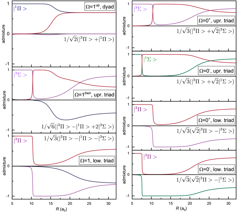
Fig.  S1: Projections of the spin-orbit-coupled Hund’s case (c) potentials onto the bare Hund’s case (a) states. The bare states are labeled near the short-range below the crossing points of about $7.5\,\textrm{a}_{0}$ and $11\,\textrm{a}_{0}$. The long-range state composition is indicated by the formulas. For simplicity the full representations of the symmetry of the states for the cases of $\Omega$ doubling as well as for the $\textrm{b}^{3}\Pi$ state are omitted. The $\Omega=2$ state is not shown, since it does not couple

S2 Classical inner and outer turning points of the ${\textrm{B}^{1}\Pi}$ potential

Table S2:  Fully empirical based RKR representation of the $\textrm{B}^{1}\Pi$ potential of the ${}^{6}\textrm{Li}{}^{40}\textrm{K}$ molecule. The table contains the calculated classical inner and outer turning points with respective vibrational energies and rotational constants. Counting of the vibrational level index is downwards from the dissociation threshold

-v	$\textrm{R}_{\textrm{inner}}\,$(a0)	$\textrm{R}_{\textrm{outer}}\,$(a0)	$G_{v}$ (cm-1)	$B_{v}$ (cm-1)
1	5.5664	61.0125	1686.964	0.005
2	5.5666	39.4987	1686.485	0.012
3	5.5673	31.4806	1684.966	0.019
4	5.5687	26.9993	1681.840	0.027
5	5.5710	24.0573	1676.591	0.035
6	5.5744	21.9495	1668.779	0.043
7	5.5791	20.3545	1658.053	0.051
8	5.5851	19.1013	1644.174	0.060
9	5.5926	18.0886	1627.031	0.069
10	5.6014	17.2496	1606.660	0.080
11	5.6116	16.5351	1583.244	0.090
12	5.6228	15.8998	1557.101	0.102
13	5.6351	15.2831	1528.497	0.112
14	5.6487	14.6576	1496.467	0.116
15	5.6643	14.1715	1459.738	0.113
16	5.6809	13.7386	1420.279	0.114
17	5.6984	13.3072	1378.324	0.119
18	5.7171	12.8860	1333.469	0.125
19	5.7368	12.4776	1285.460	0.130
20	5.7583	12.0822	1234.096	0.136
21	5.7815	11.6983	1179.195	0.142
22	5.8067	11.3240	1120.573	0.148
23	5.8345	10.9567	1058.004	0.155
24	5.8654	10.5940	991.168	0.162
25	5.9001	10.2340	919.587	0.169
26	5.9396	9.8763	842.579	0.176
27	5.9849	9.5215	759.243	0.185
28	6.0375	9.1715	668.490	0.193
29	6.0997	8.8283	569.137	0.202
30	6.1756	8.4932	460.092	0.211
31	6.2733	8.1644	340.627	0.219
32	6.4103	7.8315	210.781	0.227
33	6.6436	7.4463	71.895	0.232
R${}_{\textrm{e}}$=7.0169 a0

References

- Quemener and Julienne 2012 G. Quemener and P. S. Julienne, Chem. Rev., 2012, 112, 4949–5011.
- Baranov et al. 2012 M. A. Baranov, M. Dalmonte, G. Pupillo and P. Zoller, Chem. Rev., 2012, 112, 5012–5061.
- Bohn et al. 2017 J. L. Bohn, A. M. Rey and J. Ye, Science, 2017, 357, 1002–1010.
- DeMille 2002 D. DeMille, Phys. Rev. Lett., 2002, 88, 067901.
- Yelin et al. 2006 S. F. Yelin, K. Kirby and R. Côté, Phys. Rev. A, 2006, 74, 050301.
- Ni et al. 2018 K. K. Ni, T. Rosenband and D. D. Grimes, Chem. Sci., 2018, 9, 6830–6838.
- Hughes et al. 2020 M. Hughes, M. D. Frye, R. Sawant, G. Bhole, J. A. Jones, S. L. Cornish, M. R. Tarbutt, J. M. Hutson, D. Jaksch and J. Mur-Petit, Phys. Rev. A, 2020, 101, 062308.
- Micheli et al. 2006 A. Micheli, G. K. Brennen and P. Zoller, Nat. Phys., 2006, 2, 341.
- Büchler et al. 2007 H. P. Büchler, E. Demler, M. Lukin, A. Micheli, N. Prokof’ev, G. Pupillo and P. Zoller, Phys. Rev. Lett., 2007, 98, 060404.
- Yao et al. 2018 N. Y. Yao, M. P. Zaletel, D. M. Stamper-Kurn and A. Vishwanath, Nat. Phys., 2018, 14, 405–410.
- Andreev et al. 2018 V. Andreev, D. G. Ang, D. DeMille, J. M. Doyle, G. Gabrielse, J. Haefner, N. R. Hutzler, Z. Lasner, C. Meisenhelder, B. R. O’Leary, C. D. Panda, A. D. West, E. P. West, X. Wu and A. Collaboration, Nature, 2018, 562, 355.
- Borkowski 2018 M. Borkowski, Phys. Rev. Lett., 2018, 120, 083202.
- Borkowski et al. 2019 M. Borkowski, A. A. Buchachenko, R. Ciurylo, P. S. Julienne, H. Yamada, Y. Kikuchi, Y. Takasu and Y. Takahashi, Sci. Rep., 2019, 9, 14807.
- Carr et al. 2009 L. D. Carr, D. DeMille, R. V. Krems and J. Ye, New J. Phys., 2009, 11, 055049.
- Balakrishnan 2016 N. Balakrishnan, J. Chem. Phys., 2016, 145, 150901.
- Yang et al. 2019 H. Yang, D.-C. Zhang, L. Liu, Y.-X. Liu, J. Nan, B. Zhao and J.-W. Pan, Science, 2019, 363, 261.
- Safronova et al. 2018 M. S. Safronova, D. Budker, D. DeMille, D. F. J. Kimball, A. Derevianko and C. W. Clark, Rev. Mod. Phys., 2018, 90, 025008.
- Cairncross and Ye 2019 W. B. Cairncross and J. Ye, Nat. Rev. Phys., 2019, 1, 510–521.
- Ni et al. 2008 K.-K. Ni, S. Ospelkaus, M. H. G. de Miranda, A. Pe’er, B. Neyenhuis, J. J. Zirbel, S. Kotochigova, P. S. Julienne, D. S. Jin and J. Ye, Science, 2008, 322, 231–235.
- Park et al. 2015 J. W. Park, S. A. Will and M. W. Zwierlein, Phys. Rev. Lett., 2015, 114, 205302.
- Takekoshi et al. 2014 T. Takekoshi, L. Reichsöllner, A. Schindewolf, J. M. Hutson, C. R. Le Sueur, O. Dulieu, F. Ferlaino, R. Grimm and H.-C. Nägerl, Phys. Rev. Lett., 2014, 113, 205301.
- Molony et al. 2014 P. K. Molony, P. D. Gregory, Z. Ji, B. Lu, M. P. Köppinger, C. R. Le Sueur, C. L. Blackley, J. M. Hutson and S. L. Cornish, Phys. Rev. Lett., 2014, 113, 255301.
- Guo et al. 2016 M. Guo, B. Zhu, B. Lu, X. Ye, F. Wang, R. Vexiau, N. Bouloufa-Maafa, G. Quéméner, O. Dulieu and D. Wang, Phys. Rev. Lett., 2016, 116, 205303.
- Voges et al. 2020 K. K. Voges, P. Gersema, M. M. Z. Borgloh, T. A. Schulze, T. Hartmann, A. Zenesini and S. Ospelkaus, Phys. Rev. Lett., 2020, 125, 083401.
- Cairncross et al. 2021 W. B. Cairncross, J. T. Zhang, L. R. B. Picard, Y. C. Yu, K. Wang and K. K. Ni, Phys. Rev. Lett., 2021, 126, 123402.
- Vitanov et al. 2017 N. V. Vitanov, A. A. Rangelov, B. W. Shore and K. Bergmann, Rev. Mod. Phys., 2017, 89, 015006.
- De Marco et al. 2019 L. De Marco, G. Valtolina, K. Matsuda, W. G. Tobias, J. P. Covey and J. Ye, Science, 2019, 363, 853.
- Anderegg et al. 2018 L. Anderegg, B. L. Augenbraun, Y. C. Bao, S. Burchesky, L. W. Cheuk, W. Ketterle and J. M. Doyle, Nat. Phys., 2018, 14, 890–893.
- Anderegg et al. 2019 L. Anderegg, L. W. Cheuk, Y. C. Bao, S. Burchesky, W. Ketterle, K. K. Ni and J. M. Doyle, Science, 2019, 365, 1156.
- He et al. 2020 X. D. He, K. P. Wang, J. Zhuang, P. Xu, X. Gao, R. J. Guo, C. Sheng, M. Liu, J. Wang, J. M. Li, G. V. Shlyapnikov and M. S. Zhan, Science, 2020, 370, 331.
- Park et al. 2015 J. W. Park, S. A. Will and M. W. Zwierlein, New J. Phys., 2015, 17, 075016.
- Zhu et al. 2016 B. Zhu, X. Li, X. He, M. Guo, F. Wang, R. Vexiau, N. Bouloufa-Maafa, O. Dulieu and D. Wang, Phys. Rev. A, 2016, 93, 012508.
- Rvachov et al. 2018 T. M. Rvachov, H. Son, J. J. Park, S. Ebadi, M. W. Zwierlein, W. Ketterle and A. O. Jamison, Phys. Chem. Chem. Phys., 2018, 20, 4739–4745.
- Brachmann 2012 J. F. S. Brachmann, Ph.D. thesis, MPQ-LMU, Munich, 2012.
- Köhler et al. 2006 T. Köhler, K. Góral and P. S. Julienne, Rev. Mod. Phys., 2006, 78, 1311–1361.
- Ridinger et al. 2011 A. Ridinger, S. Chaudhuri, T. Salez, D. R. Fernandes, N. Bouloufa, O. Dulieu, C. Salomon and F. Chevy, EPL, 2011, 96, 33001.
- Pashov et al. 1998 A. Pashov, W. Jastrzȩbski and P. Kowalczyk, Chem. Phys. Lett, 1998, 292, 615–620.
- Rydberg 1933 R. Rydberg, Z. Phys., 1933, 80, 514–524.
- Klein 1932 O. Klein, Z. Phys., 1932, 76, 226–235.
- Rees 1947 A. Rees, Proc. Phys. Soc., 1947, 59, 998–1008.
- Taglieber et al. 2008 M. Taglieber, A.-C. Voigt, T. Aoki, T. W. Hänsch and K. Dieckmann, Phys. Rev. Lett., 2008, 100, 010401.
- Voigt et al. 2009 A.-C. Voigt, M. Taglieber, L. Costa, T. Aoki, W. Wieser, T. W. Hänsch and K. Dieckmann, Phys. Rev. Lett., 2009, 102, 020405.
- Yang et al. 2020 A. Yang, S. Botsi, S. Kumar, S. B. Pal, M. M. Lam, I. Cepaite, A. Laugharn and K. Dieckmann, Phys. Rev. Lett., 2020, 124, 133203.
- Ridinger 2011 A. Ridinger, Ph.D. thesis, ENS Paris, Munich, 2011.
- Tiemann et al. 2009 E. Tiemann, H. Knöckel, P. Kowalczyk, W. Jastrzebski, A. Pashov, H. Salami and A. J. Ross, Phys. Rev. A, 2009, 79, 042716.
- 46 Website of A.R. Allouche, https://sites.google.com/site/allouchear/Home/diatomic.
- Brachmann et al. 2012 J. F. S. Brachmann, T. Kinder and K. Dieckmann, Appl. Opt., 2012, 51, 5517–5521.
- Brown and Carrington 2003 J. M. Brown and A. Carrington, in Rotational Spectroscopy of Diatomic Molecules, Cambridge University Press, 2003, ch. 10.7.1., p. 813.
- Carrington et al. 1995 A. Carrington, C. Leach, A. Marr, A. Shaw, M. Viant, J. Hutson and M. Law, J. Chem. Phys., 1995, 102, 2379–2403.
- Schadee 1978 A. Schadee, J. Quant. Spectrosc. Radiat. Transf., 1978, 19, 517–531.
- LeRoy and Bernstein 1970 R. J. LeRoy and R. B. Bernstein, J. Chem. Phys., 1970, 52, 3869–3879.
- Leroy and Bernstein 1970 R. J. Leroy and R. B. Bernstein, Chem. Phys. Lett., 1970, 5, 42–44.
- Falke et al. 2006 S. Falke, E. Tiemann, C. Lisdat, H. Schnatz and G. Grosche, Phys. Rev. A, 2006, 74, 032503.
- Tromp and LeRoy 1985 J. Tromp and R. LeRoy, J. Mol. Spectrosc., 1985, 109, 352–367.
- Appadoo et al. 1996 D. Appadoo, R. LeRoy, P. Bernath, S. Gerstenkorn, P. Luc, J. Verges, J. Sinzelle, J. Chevillard and Y. Daignaux, J. Chem. Phys., 1996, 104, 903–913.
- LeRoy 1972 R. LeRoy, Can. J. Phys., 1972, 50, 953.
- Goscinski and Tapia 1972 O. Goscinski and O. Tapia, Mol. Phys., 1972, 24, 641.
- LeRoy 1980 R. J. LeRoy, J. Chem. Phys., 1980, 73, 6003–6012.
- Comparat 2004 D. Comparat, J. Chem. Phys., 2004, 120, 1318–1329.
- Bussery et al. 1987 B. Bussery, Y. Achkar and M. Aubert-Frécon, Chem. Phys., 1987, 116, 319–338.
- Ji et al. 1995 B. Ji, C. C. Tsai and W. C. Stwalley, Chem. Phys. Lett., 1995, 236, 242–246.
- Li et al. 2019 C. Y. Li, W. L. Liu, J. Z. Wu, X. F. Wang, Y. Q. Li, J. Ma, L. T. Xiao and S. T. Jia, J. Quant. Spectrosc. Radiat. Transf., 2019, 225, 214–218.
- Le Roy 2017 R. J. Le Roy, J. Quant. Spectrosc. Radiat. Transf., 2017, 186, 158–166.

References

- Tiecke et al. 2010 T. G. Tiecke, M. R. Goosen, J. T. M. Walraven and S. J. J. M. F. Kokkelmans, Phys. Rev. A, 2010, 82, 042712.
- Yang et al. 2020 A. Yang, S. Botsi, S. Kumar, S. B. Pal, M. M. Lam, I. Cepaite, A. Laugharn and K. Dieckmann, Phys. Rev. Lett., 2020, 124, 133203.
- 3 Website of A.R. Allouche, https://sites.google.com/site/allouchear/Home/diatomic.