Minimal mass blow-up solutions for the $L^{2}$-critical NLS with the Delta potential for radial data in one dimension

Abstract.

We consider the $L^{2}$-critical nonlinear Schrödinger equation (NLS) with the delta potential

$$i\partial_{t}u+\partial^{2}_{x}u+\mu\delta u+|u|^{4}u=0,\,\,t\in\mathbb{R},\,x\in\mathbb{R},$$

where $\mu\in\mathbb{R}$, and $\delta$ is the Dirac delta distribution at $x=0$. Local well-posedness theory together with sharp Gagliardo-Nirenberg inequality and the conservation laws of mass and energy implies that the solution with mass less than $\|Q\|_{2}$ is global existence in $H^{1}(\mathbb{R})$, where $Q$ is the ground state of the $L^{2}$-critical NLS without the delta potential (i.e. $\mu=0$).

We are interested in the dynamics of the solution with threshold mass $\|u_{0}\|_{2}=\|Q\|_{2}$ in $H^{1}(\mathbb{R})$. First, for the case $\mu=0$, such blow-up solution exists due to the pseudo-conformal symmetry of the equation, and is unique up to the symmetries of the equation in $H^{1}(\mathbb{R})$ from [49] (see also [30]), and recently in $L^{2}(\mathbb{R})$ from [17]. Second, for the case $\mu<0$, simple variational argument with the conservation laws of mass and energy implies that radial solutions with threshold mass exist globally in $H^{1}(\mathbb{R})$. Last, for the case $\mu>0$, we show the existence of radial threshold solutions with blow-up speed determined by the sign (i.e. $\mu>0$) of the delta potential perturbation since the refined blow-up profile to the rescaled equation is stable in a precise sense. The key ingredients here including the Energy-Morawetz argument and compactness method as well as the modulation analysis are close to the original one in [61] (see also [34, 39, 42, 46, 55]).

1. Introduction

In this paper, we consider the $L^{2}$-critical nonlinear Schrödinger equation with the delta potential

$$\begin{cases}i\partial_{t}u+\partial^{2}_{x}u+\mu\delta u+|u|^{4}u=0,&(t,x)\in\mathbb{R}\times\mathbb{R},\\ u(0,x)=u_{0}(x)\in H^{1}(\mathbb{R}),&\end{cases}$$ (1.1)

where $u$ is a complex-valued function of $(t,x)$, $\mu\in\mathbb{R}$, $\delta$ is the Dirac delta distribution at the origin. For $\mu=0$, it is focusing, $L^{2}$-critical nonlinear Schrödinger equation (NLS) in one dimension, here we call it the $L^{2}$-critical NLS since the scaling transformation

$$u_{\lambda}(t,x)=\lambda^{\frac{1}{2}}u(\lambda^{2}t,\lambda x)$$

leaves the $L^{2}$ norm invariant

$$\|u_{\lambda}(t,\cdot)\|_{2}=\|u(\lambda^{2}t,\cdot)\|_{2}.$$

A series of studies dealt with the $L^{2}$-critical NLS, we can refer to [7, 13, 16, 17, 22, 49, 62], and references therein. For $\mu\not=0$, it appears in various physical models with a point defect on the line, for instance, quantum mechanics [2], nonlinear optics [25, 28, 29] and references therein. We can refer to [1, 2] for more details on the $\delta$-perturbation of strength $\mu$ of the self-adjoint operator $\partial^{2}_{x}$. The appearance of the delta potential destroys spatial translation, scaling transformation and pseudo-conformal transformation invariances of (1.1). For the case $\mu<0$, it corresponds to the repulsive delta potential, while for the case $\mu>0$, it corresponds to the attractive delta potential.

Local well-posedness result for (1.1) is well understood in $H^{1}(\mathbb{R})$ by many authors, for example, by Cazenave in [7, Theorem 3.7.1], Fukuizumi, Ohta and Ozawa in [24] and Masaki, Murphy and Segata in [47]. More precisely, we have

Proposition 1.1.

For any $u_{0}\in H^{1}(\mathbb{R})$, there exists a unique maximal lifespan solution $u\in\mathcal{C}\left(\left(-T_{*},T^{*}\right),H^{1}(\mathbb{R})\right)\cap\mathcal{C}^{1}\left(\left(-T_{*},T^{*}\right),H^{-1}(\mathbb{R})\right)$ of (1.1) satisfying the the following blow-up criterion,

$$T^{*}<+\infty\text{\;implies that\;}\displaystyle\lim\limits_{t\nearrow T^{*}}\lVert\partial_{x}u(t)\rVert_{2}=+\infty.$$ (1.2)

Moreover, the mass and the energy are conserved under the flow (1.1), i.e., for any $t\in\left(-T_{*},T^{*}\right)$, we have

$$M(u(t)):=\frac{1}{2}\int_{\mathbb{R}}|u(t,x)|^{2}dx=M(u_{0}),$$ (1.3)

$$E(u(t)):=\int_{\mathbb{R}}\left[\frac{1}{2}|\partial_{x}u(t,x)|^{2}-\frac{1}{2}\mu\ \delta(x)|u(t,x)|^{2}-\frac{1}{6}|u(t,x)|^{6}\right]dx=E(u_{0}).$$ (1.4)

1.1. The $L^{2}$-critical case $\mu=0$.

Let us firstly recall the well-known results of (1.1) for the case $\mu=0$. From the variational argument in [65], the positive, radial ground state solution to

$$-\partial^{2}_{x}Q+Q-|Q|^{4}Q=0,\ \ Q\in H^{1}(\mathbb{R}),\ \ Q>0,\ \ \mbox{$Q$ radial}$$ (1.5)

is the extremizer of sharp Gagliardo-Nirenberg inequality

$$\|u\|^{6}_{6}\leq C_{\rm GN}\|u\|_{2}^{4}\|\partial_{x}u\|_{2}^{2},$$ (1.6)

where $C_{\rm GN}=3/\lVert Q\rVert^{4}_{2}$. Moreover, the ground state $Q$ is unique up to symmetries of (1.5) from [5, 37]. Therefore, for any $u\in H^{1}(\mathbb{R})$, we have

$$E(u)=E_{\rm crit}(u):=\frac{1}{2}\lVert\partial_{x}u\rVert_{2}^{2}-\frac{1}{6}\lVert u\rVert_{6}^{6}\geq\frac{1}{2}\|\partial_{x}u\|_{2}^{2}\left(1-\frac{\|u\|^{4}_{2}}{\|Q\|^{4}_{2}}\right),$$ (1.7)

which together with (1.3), (1.4) and the blow-up criterion (1.2) implies that the solutions of (1.1) with mass less than $\|Q\|_{2}$ globally exist in $H^{1}(\mathbb{R})$. Furthermore, it scatters to the linear solutions $e^{it\partial^{2}_{x}}u^{\pm}_{0}$ for some $u^{\pm}_{0}\in L^{2}(\mathbb{R})$ in both time directions in $L^{2}(\mathbb{R})$, we can refer to [13] for more details.

For the critical mass case $\|u_{0}\|_{2}=\|Q\|_{2}$. By applying the pseudo-conformal transformation

$$u(t,x)\longmapsto v(t,x)=\frac{1}{|t|^{\frac{1}{2}}}\bar{u}\left(\frac{1}{t},\frac{x}{t}\right)e^{i\frac{|x|^{2}}{4t}}$$ (1.8)

to the solitary solution $u(t,x)=Q(x)e^{it}$, we can obtain the explicit blow-up solution with threshold mass

$$S(t,x)=\frac{1}{|t|^{\frac{1}{2}}}Q\left(\frac{x}{|t|}\right)e^{-i\frac{|x|^{2}}{4|t|}}e^{\frac{i}{|t|}},\quad\|S(t)\|_{2}=\|Q\|_{2},\quad\text{and}\quad\|\partial_{x}S(t)\|_{2}\approx\frac{1}{|t|}\,\,\text{as}\,\,t\to 0^{-}.$$ (1.9)

From [49], finite time blow-up solutions with threshold mass $\lVert Q\rVert_{2}$ are completely classified by F. Merle in $H^{1}(\mathbb{R})$ in the following sense

$$\|u(t,\cdot)\|_{2}=\|Q\|_{2}\ \ \mbox{and}\ \ T^{*}<+\infty\ \ \mbox{imply}\ \ u\equiv S$$

up to the symmetries of (1.1) (see also [30] for simplified proof). Recently B. Dodson pushes this rigidity result forward in [17, 18], and obtains the classification result of finite time blow-up solutions of the focusing, $L^{2}$-critical NLS with threshold mass in $L^{2}(\mathbb{R}^{d})$, $1\leq d\leq 15$.

For the super-critical mass case $\|u_{0}\|_{2}>\|Q\|_{2}$, there are lots of important blow-up results of (1.1) in $H^{1}(\mathbb{R})$, we can refer to [6, 21, 50, 51, 52, 53, 54, 58, 59, 60], and references therein.

1.2. The repulsive potential case $\mu<0$

Now we consider the repulsive potential case $\mu<0$. On the one hand, there are no solitary waves of (1.1) with the subcritical mass $\|u_{0}\|_{2}<\|Q\|_{2}$ from classical variational argument in [24, 38]. On the other hand, by (1.3), (1.4) and sharp Gagliardo-Nirenberg inequality (1.6), we can obtain similar estimate to those in (1.7)

$$E(u(t))=\frac{1}{2}\lVert\partial_{x}u(t,\cdot)\rVert_{2}^{2}-\frac{\mu}{2}|u(t,0)|^{2}-\frac{1}{6}\lVert u(t,\cdot)\rVert_{6}^{6}\geq\frac{1}{2}\|\partial_{x}u(t,\cdot)\|_{2}^{2}\left(1-\frac{\|u(t,\cdot)\|^{4}_{2}}{\|Q\|^{4}_{2}}\right).$$

This together with the blow-up criterion (1.2) implies the global existence of the solutions of (1.1) with mass less than $\|Q\|_{2}$ in $H^{1}(\mathbb{R})$. Because of the repulsive ($\mu<0$) delta potential perturbation and the lack of the pseudo-conformal symmetry (1.8), we have at the threshold mass that

Theorem 1.2.

Let $\mu<0$, and radial $u_{0}\in H^{1}(\mathbb{R})$ with $\|u_{0}\|_{2}=\|Q\|_{2}$, then the solution of (1.1) is global and bounded in $H^{1}(\mathbb{R})$.

The result follows from the standard concentration compactness argument with the conservation laws of mass and energy, see proof in Appendix A.

In contrast to the subcritical mass, there are solitary waves $Q_{\omega,\mu}(x)e^{i\omega t}$ of (1.1) with the super-critical mass $\|Q_{\omega,\mu}\|_{2}>\|Q\|_{2}$ from standard variational argument in [24, 38], at the same time, these solitary waves are orbitally unstable, and even strongly unstable in $H^{1}(\mathbb{R})$, we can refer to [38], and references therein. Therefore the global existence result in Theorem 1.2 is sharp in $H^{1}(\mathbb{R})$, and we also conjecture that for the repulsive delta potential case, the solutions of (1.1) with $\lVert u_{0}\rVert_{2}\leq\lVert Q\rVert_{2}$ will scatter to the linear solution in both time directions in $L^{2}(\mathbb{R})$ due to the result in [13]. For other long-time asymptotic behavior and scattering results of nonlinear Schrödinger equation with the repulsive delta potential, we can refer to [4, 12, 31, 47], and references therein.

1.3. The attractive potential case $\mu>0$

Let us now turn to the attractive potential case $\mu>0$, it is main part for the rest of the paper. First, by the Sobolev inequality and the Young inequality, we have for any $u\in H^{1}(\mathbb{R})$ with $\lVert u\rVert_{2}<\lVert Q\rVert_{2}$ that

$$\frac{\mu}{2}|u(t,0)|^{2}\leq\frac{\mu}{2}\lVert\partial_{x}u(t,\cdot)\rVert_{2}\lVert u(t,\cdot)\rVert_{2}\leq\frac{1}{6}\|\partial_{x}u\|_{2}^{2}\left(1-\frac{\|u(t,\cdot)\|^{4}_{2}}{\|Q\|^{4}_{2}}\right)+C(\mu,\lVert u(t,\cdot)\rVert_{2}),$$

this together with sharp Gagliardo-Nirenberg inequality (1.6) implies that for any $u\in H^{1}(\mathbb{R})$, we have

$$E(u(t))=\frac{1}{2}\lVert\partial_{x}u(t,\cdot)\rVert_{2}^{2}-\frac{\mu}{2}|u(t,0)|^{2}-\frac{1}{6}\lVert u(t,\cdot)\rVert_{6}^{6}\\ \geq\frac{1}{3}\|\partial_{x}u(t,\cdot)\|_{2}^{2}\left(1-\frac{\|u(t,\cdot)\|^{4}_{2}}{\|Q\|^{4}_{2}}\right)-C(\mu,\lVert u(t,\cdot)\rVert_{2}),$$ (1.10)

which once again implies the controllability of the kinetic energy $\lVert\partial_{x}u(t)\rVert^{2}_{2}$ of the solution of (1.1) by the mass and energy, and deduces global well-posedness of the solution of (1.1) with $\|u_{0}\|_{2}<\|Q\|_{2}$ in $H^{1}(\mathbb{R})$ due to (1.3), (1.4) and the blow-up criterion (1.2). However, in contrast to both the case $\mu=0$ and the case $\mu<0$, there exist arbitrarily small solitary waves $Q_{\omega,\mu}(x)e^{i\omega t}$ as follows,

Proposition 1.3.

Let $\mu>0$. For all $M\in(0,\|Q\|_{2})$, there exists $\omega>\mu^{2}/4$ and a unique positive, radially symmetric solution of

$$-\omega Q_{\omega,\mu}+\partial^{2}_{x}Q_{\omega,\mu}+\mu\delta Q_{\omega,\mu}+Q_{\omega,\mu}^{5}=0,\ \ \|Q_{\omega,\mu}\|_{2}=M.$$

The proof of Proposition 1.3 follows from classical variational argument in [23, 24], we give alternative proof by in Appendix B. Since the solitary waves $Q_{\omega,\mu}(x)e^{i\omega t}$ themselves don’t scatter to the linear solution, the solution of (1.1) with mass less than $\lVert Q\rVert_{2}$ don’t scatter in $L^{2}(\mathbb{R})$ any more in this case. The necessary condition that $\omega>\mu^{2}/4$ is related to the eigenvalue of the Schrödigner operator $\partial^{2}_{x}+\mu\delta$ in [2, 24]. In fact, these solitary waves can be explicitly described as following (see [24, 25])

$${Q}_{\omega,\mu}(x)=\left[3\omega\operatorname{sech}^{2}\left(2\sqrt{\omega}|x|+\operatorname{arctanh}\left(\frac{\mu}{2\sqrt{\omega}}\right)\right)\right]^{\frac{1}{4}}.$$ (1.11)

By the well-known stability theory in [8, 24, 27], these solitary waves are orbitally stable in $H^{1}(\mathbb{R})$.

In contrast to the non-existence result of finite time blow-up solutions with threshold mass for the repulsive case $\mu<0$ in Theorem 1.2, the main goal of this paper is to show the existence of finite time blow-up solutions of (1.1) with threshold mass in the attractive case $\mu>0$ as follows,

Theorem 1.4.

Let $\mu>0$ and $E_{0}\in\mathbb{R}$, there exist $t_{0}<0$ and a radial data $u(t_{0})\in H^{1}(\mathbb{R})$ with

$$\|u(t_{0})\|_{2}=\|Q\|_{2},\ \ E(u(t_{0}))=E_{0},$$

such that the corresponding solution $u(t)$ of (1.1) blows up at time $T^{*}=0$ with the blow-up speed:

$$\|\partial_{x}u(t)\|_{2}\approx\frac{1}{|t|^{2/3}},\quad\text{as}\quad t\to 0^{-}.$$ (1.12)

Remark 1.5.

We give some remarks on this result.

1. Energy. Minimal mass blow-up solutions in Theorem 1.4 have arbitrary energy $E_{0}\in\mathbb{R}$, which is different with the positive energy $E_{\rm crit}(S(t))$of the explicit pseudo-conformal blow-up solution $S(t,x)$ in (1.9).

2. Blow-up speed. The blow-up speed $|t|^{-2/3}$ in (1.12) is different with the pseudo-conformal blow-up speed $|t|^{-1}$ in (1.9), the self similar blow-up speed ${|t|^{-\frac{1}{2}}}$ and the log-log blow-up speed for $L^{2}$-critical NLS in [6, 50, 51, 52, 53, 57]. The possible blow-up speed for the critical problem is an interesting problem, we can refer [43, 44, 45] for the $L^{2}$-critical KdV equation, [35, 36] for the $\dot{H}^{1}$-critical wave equation and references therein.

3. Profile. The analysis provides the following profile of minimal mass blow-up solution

   $$u(t,x)=\frac{1}{\lambda^{\frac{1}{2}}(t)}Q\left(\frac{x}{\lambda(t)}\right)e^{-i\frac{2}{3}\frac{|x|^{2}}{4t}}e^{i\gamma(t)}+v\left(t,{x}\right)$$ (1.13)

   where $Q$ is the ground state solution of $L^{2}$-critical NLS, and

   $$\lim_{t\rightarrow 0}\lVert v(t)\rVert_{2}=0,\quad\text{and}\quad\lambda(t)\approx C{|t|^{2/3}},\quad\text{as}\quad t\to 0^{-}.$$

   See (4.6) and (4.7).

4. Uniqueness. The uniqueness of minimal mass blow-up solution is an important problem, which is closely related to classify the compact elements of the flow in the Kenig-Merle’s concentration-compactness-rigidity argument [32], we can also refer to [17, 18, 19, 20, 33, 40, 56, 64], and references therein.

The results in Theorem 1.2 and Theorem 1.4 show the completely different consequence determined by the delta potentials in the existence of minimal mass blow-up solutions of (1.1) in $H^{1}(\mathbb{R})$. Due to the refined blow-up profile to the rescaled equation is stable in a very precise sense, the construction proof of Theorem 1.4 using the Energy-Morawetz argument and compactness method as well as the modulation analysis is close to the original non perturbative argument in [61] (see also [34, 39, 42, 46]), which is different with the perturbation argument in [3]. More precisely, we adapts the compactness argument under the uniform estimates for the special solution on sufficiently far away time rescaled interval, which in fact can be satisfied by modulation analysis, the Energy-Morawetz estimate of the remainder term $\varepsilon(t,x)$ and the bootstrap argument. The related application of the Energy-Morawetz estimate in the blow-up dynamics can also be found in [55, 61]. The Energy-Morawetz estimate is also successfully applied by B. Dodson in [14, 15] to obtain the global well-posedness and scattering result for the radial solution of the defocusing, nonlinear wave equation in the critical Sobolev space $\dot{H}^{s}(\mathbb{R}^{3})$ for $\frac{1}{2}\leq s<1$.

For other results of nonlinear Schrödinger equation with the attractive delta potential in $H^{1}(\mathbb{R})$, we can refer to [24, 25, 38, 48, 63] and references therein for the stability analysis of the solitary waves.

1.4. Notation

Let us collect the notation and some well-known facts used in this paper. Throughout the paper, we use the notation $X\lesssim Y$, or $Y\gtrsim X$ to denote the statement that $X\leq CY$ for some constant $C$, which may vary from line to line. We use $X=O(Y)$ synonymously with $|X|\lesssim Y$. We use $X\approx Y$ to denote the statement $X\lesssim Y\lesssim X$.

Since the appearance of the Dirac delta potential destroys spatial translation invariance of (1.1) for $\mu>0$, we only deal with the radial case. The $L^{2}$ scalar product and $L^{r}$ norm ($r\geq 1$) are denoted by

$$\left(u,v\right)_{2}=\mathrm{Re}\left(\int_{\mathbb{R}}u(x)\bar{v}(x)\,dx\right),\quad\|u\|_{r}=\left(\int_{\mathbb{R}}|u|^{r}\,dx\right)^{\frac{1}{r}}.$$

We denote the radial functions in $H^{1}(\mathbb{R})$ by $H^{1}_{\rm rad}(\mathbb{R})$.

We fix the notation: for $\mu>0$, $u\in\mathbb{C}$, denote

$$f(u)=|u|^{4}u;\quad g(u)=\mu\,\delta u;\quad F(u)=\frac{1}{6}|u|^{6};\quad G(u)=\frac{1}{2}\mu\,\delta|u|^{2}.$$

where $\delta=\delta(x)$ is the Dirac delta distribution at the origin and obeys the following scaling property by simple distribution calculation (see [26]):

$$\forall x\in\mathbb{R},\ \lambda>0,\quad\delta(\lambda x)=\frac{1}{\lambda}\delta(x).$$ (1.14)

Identifying $\mathbb{C}$ with $\mathbb{R}^{2}$, we denote the Fréchet-derivative of functions $f,g,F,G$ by $df$, $dg$, $dF$ and $dG$. Let $\Lambda$ be the infinitesimal generator of the $L^{2}$-scaling transformation, i.e.

$$\Lambda=\frac{1}{2}+y\cdot\partial_{y}.$$

Without loss of generality, we may assume that $\mu^{2}/4<\omega=1$ in the rest of the paper, the linearized operator around $Qe^{it}$ is

$$L_{+}:=-\partial^{2}_{y}+1-5Q^{4},\qquad L_{-}:=-\partial^{2}_{y}+1-Q^{4}.$$

and the generalized kernel of

$$\begin{pmatrix}0&L_{-}\\ -L_{+}&0\end{pmatrix}$$

is non-degenerate and spanned by the symmetries of the equation (see [37, 66] and [10]). It is described in $H^{1}_{\rm rad}(\mathbb{R})$ by the algebraic relations (we define $\rho$ as the unique radial solution to $L_{+}\rho=|y|^{2}Q$)

$$L_{-}Q=0,\quad L_{+}\Lambda Q=-2Q,\quad L_{-}|y|^{2}Q=-4\Lambda Q,\quad L_{+}\rho=|y|^{2}Q.$$ (1.15)

From these algebraic relations, we have

$$\left(Q,\rho\right)_{2}=-\frac{1}{2}\left(L_{+}\Lambda Q,\rho\right)_{2}=-\frac{1}{2}\left(\Lambda Q,L_{+}\rho\right)_{2}=-\frac{1}{2}\left(\Lambda Q,|y|^{2}Q\right)_{2}=\frac{1}{2}\lVert yQ\rVert^{2}_{2}.$$ (1.16)

Denote by $\mathcal{Y}$ the set of radially symmetric functions $f\in\mathcal{C}^{\infty}(\mathbb{R}\backslash\{0\})$ such that

$$\forall\alpha\in\mathbb{N},\quad\exists C_{\alpha},\ \kappa_{\alpha}>0,\ \forall x\in\mathbb{R}\backslash\{0\},\quad|\partial^{\alpha}f(x)|\leq C_{\alpha}(1+|x|)^{\kappa_{\alpha}}Q(x).$$

It follows from the kernel properties of $L_{+}$ and $L_{-}$, and [11, Appendix A] or proof of Lemma 3.2 in [55] for related arguments) that

$$\forall g\in\mathcal{Y},\ \exists f_{+}\in\mathcal{Y},\ L_{+}f_{+}=g,$$ (1.17)

$$\forall g\in\mathcal{Y},\ \left(g,Q\right)_{2}=0,\ \exists f_{-}\in\mathcal{Y},\ L_{-}f_{-}=g.$$ (1.18)

For the sake of the localization argument in Section 3, We introduce the localized function $\phi$ and its scaling. Let $\phi:\mathbb{R}\to\mathbb{R}$ be a smooth even and convex function, nondecreasing on $\mathbb{R}^{+}$, such that

$$\phi(r)=\left\{\begin{aligned} &\frac{1}{2}r^{2}&\text{ for }&r<1,\\ &3r+e^{-r}&\text{ for }&r>2,\end{aligned}\right.$$

and set $\phi(x)=\phi(|x|)$. For $A\gg 1$, define $\phi_{A}$ by $\phi_{A}(x)=A^{2}\phi\left(\frac{x}{A}\right)$.

This paper is organized as follows. In Section 2, we construct the refined blow-up profile by according to the Dirac potential perturbation, and obtain the approximate blow-up law affected by the Dirac potential perturbation. In Section 3, we obtain the uniform backwards estimates of the remainder $\varepsilon$ and modulation parameters $\lambda,b$ on the rescaled time interval by combining the modulation analysis, the Energy-Morawetz argument with the bootstrap argument on the sufficiently far away rescaled time interval. In Section 4, we can construct minimal mass blow-up solution by combining the compactness argument with the uniform backwards estimates in Section 3. In Appendix A, we use the variational argument, and the conservation laws of mass and energy to show the global existence of radial solution of (1.1) with threshold mass for the repulsive potential case $\mu<0$ in $H^{1}(\mathbb{R})$. In Appendix B, we use the variational argument to show Proposition 1.3, that is, the existence of arbitrarily small radial soliton solutions of (1.1) for the attractive potential case $\mu>0$.

Acknowledgements.

G. Xu was supported by National Key Research and Development Program of China (No. 2020YFA0712900) and by NSFC (No. 11831004). X. Tang was supported by NSFC (No. 12001284).

2. Construction of the refined blow-up profile

In this section, we construct the refined blow-up profile according to the Dirac delta potential perturbation.

2.1. Refined blow-up profile

We start with the heuristic argument justifying the construction as that in [61] (see also [34] [39] [46]). Since the Dirac delta potential term $\mu\delta u$ destroys the invariances of spatial translation and Galilean transformation of (1.1), we try to look for a solution with the structure

$$u(t,x)=\frac{1}{\lambda^{\frac{1}{2}}(s)}w(s,y)e^{i\gamma(s)-i\frac{b(s)|y|^{2}}{4}},\qquad\frac{ds}{dt}=\frac{1}{\lambda^{2}},\qquad y=\frac{x}{\lambda(s)},$$ (2.1)

where $(s,y)$ are the rescaled variables, and the parameters $\lambda>0,b,\gamma$ is to be determined later. By inserting (2.1) into (1.1), the profile function $w$, and $\lambda$, $b$ and $\gamma$ should satisfy the following rescaled equation

$$iw_{s}+\partial^{2}_{y}w-w+f(w)+\lambda g(w)\\ -i\left(\frac{\lambda_{s}}{\lambda}+b\right)\Lambda w+(1-\gamma_{s})w+(b_{s}+b^{2})\frac{|y|^{2}}{4}w-b\left(b+\frac{\lambda_{s}}{\lambda}\right)\frac{|y|^{2}}{2}w=0.$$ (2.2)

where we used the fact that (1.14). Since we look for the blow-up solution, the parameter $\lambda(s)$ should converge to zero as $s\to\infty$. Therefore, we expect that the parameters $\lambda$, $b$, $\gamma$ satisfy the modulation equations

$$\frac{\lambda_{s}}{\lambda}+b=0,\quad b_{s}+b^{2}=0,\quad 1-\gamma_{s}=0,$$ (2.3)

and that

$$w(s,y)=Q(y)$$ (2.4)

is an approximate solution of (2.2) with zero order term of $\lambda$ and $b$. However, the first order error term $\lambda g(Q)$ cannot be regarded as small perturbation in minimal blow-up analysis due to the slow variation property of the parameter $\lambda$ (In fact $\lambda(s)\approx s^{-2}$ for sufficiently large $s$, see Lemma 2.3 and (3.7) in Proposition 3.2). We rewrite (2.2) as follows

$$iw_{s}+\partial^{2}_{y}w-w+f(w)+\lambda g(w)+\theta\frac{|y|^{2}}{4}w\\ -i\left(\frac{\lambda_{s}}{\lambda}+b\right)\Lambda w+(1-\gamma_{s})w+(b_{s}+b^{2}-\theta)\frac{|y|^{2}}{4}w-b\left(\frac{\lambda_{s}}{\lambda}+b\right)\frac{|y|^{2}}{2}w=0,$$ (2.5)

where $\theta$ is determined later and the additional term $\theta|y|^{2}w/4$ is introduced to construct the refined blow-up profile $P(s,y)$ with higher order terms of $\lambda$ and $b$ in Proposition 2.1 (In fact, it is related to the solvability of the linearized operators $L_{\pm}$ in (2.22)), and will modify the modulation equations in (2.3), and is responsible for the blow-up result obtained in Theorem 1.4.

Fix $K\in\mathbb{N}$, $K\geq 7$ is sufficient in the proof of Theorem 1.4, and define

$$\Sigma_{K}=\{(j,k)\in\mathbb{N}^{2}\ |\ j+k\leq K\}.$$

Proposition 2.1.

Let $\lambda(s)>0$ and $b(s)\in\mathbb{R}$ be $\mathcal{C}^{1}$ functions of $s$ such that $\lambda(s)+|b(s)|\ll 1$.
(i) Existence of a refined blow-up profile. For any $(j,k)\in\Sigma_{K}$, there exist real-valued functions $P_{j,k}^{\pm}\in\mathcal{Y}$ and $\beta_{j,k}\in\mathbb{R}$ such that $P(s,y)=\tilde{P}_{K}(y;b(s),\lambda(s))$, where $\tilde{P}_{K}$ is defined by

$$\tilde{P}_{K}(y;b,\lambda):=Q(y)+\sum_{(j,k)\in\Sigma_{K}}b^{2j}\lambda^{k+1}P_{j,k}^{+}(y)+i\sum_{(j,k)\in\Sigma_{K}}b^{2j+1}\lambda^{k+1}P_{j,k}^{-}(y)$$ (2.6)

satisfies

$$i\partial_{s}P+\partial^{2}_{y}P-P+f(P)+\lambda g(P)+\theta\frac{|y|^{2}}{4}P=\Psi_{K},$$ (2.7)

where $\theta(s)=\tilde{\theta}(b(s),\lambda(s))$ is defined by

$$\tilde{\theta}(b,\lambda)=\sum_{(j,k)\in\Sigma_{K}}b^{2j}\lambda^{k+1}\beta_{j,k},$$ (2.8)

and $\Psi_{K}$ satisfies

$$\sup_{y\in\mathbb{R}}\left(e^{\frac{|y|}{2}}\left(|\Psi_{K}(y)|+|\partial_{y}\Psi_{K}(y)|\right)\right)\lesssim\lambda\left(\Big{|}\frac{\lambda_{s}}{\lambda}+b\Big{|}+\left|b_{s}+b^{2}-\theta\right|\right)+(|b|^{2}+\lambda)^{K+2}.$$ (2.9)

(ii) Rescaled blow-up profile. Let

$$P_{b}(s,y)=P(s,y)e^{-i\frac{b(s)|y|^{2}}{4}},$$ (2.10)

then we have

$$i\partial_{s}P_{b}+\partial^{2}_{y}P_{b}-P_{b}+f(P_{b})+\lambda g(P_{b})-i\frac{\lambda_{s}}{\lambda}\Lambda P_{b}\\ =-i\left(\frac{\lambda_{s}}{\lambda}+b\right)\Lambda P_{b}+(b_{s}+b^{2}-\theta)\frac{|y|^{2}}{4}P_{b}+\Psi_{K}e^{-i\frac{b|y|^{2}}{4}}.$$ (2.11)

(iii) Mass and energy properties of the blow-up profile. Let

$$P_{b,\lambda,\gamma}(s,y)=\frac{1}{\lambda^{\frac{1}{2}}}P_{b}\left(s,y\right)e^{i\gamma},$$ (2.12)

then we have

$$\left|\frac{d}{ds}\int_{\mathbb{R}}|P_{b,\lambda,\gamma}|^{2}\,dy\right|\lesssim\lambda\left(\Big{|}\frac{\lambda_{s}}{\lambda}+b\Big{|}+\left|b_{s}+b^{2}-\theta\right|\right)+(|b|^{2}+\lambda)^{K+2},$$ (2.13)

$$\left|\frac{d}{ds}{E(P_{b,\lambda,\gamma})}\right|\lesssim\frac{1}{\lambda^{2}}\left(\Big{|}\frac{\lambda_{s}}{\lambda}+b\Big{|}+\left|b_{s}+b^{2}-\theta\right|+(|b|^{2}+\lambda)^{K+2}\right).$$ (2.14)

Moreover, for any $(j,k)\in\Sigma_{K},$ there exist $\eta_{j,k}\in\mathbb{R}$ such that

$$\left|E(P_{b,\lambda,\gamma})-\frac{1}{8}\cdot\mathcal{E}(b,\lambda)\cdot\int|y|^{2}Q^{2}dy\right|\lesssim\frac{(b^{2}+\lambda)^{K+2}}{\lambda^{2}},$$ (2.15)

where

$$\mathcal{E}(b,\lambda)=\frac{b^{2}}{\lambda^{2}}-2\beta\frac{\lambda}{\lambda^{2}}+\frac{\lambda}{\lambda^{2}}\sum_{(j,k)\in\Sigma_{K},j+k\geq 1}b^{2j}\lambda^{k}\eta_{j,k},\quad\beta=2\mu\frac{Q(0)^{2}}{\lVert yQ\rVert_{2}^{2}}=4\frac{G(Q)}{\lVert yQ\rVert^{2}_{2}}>0.$$ (2.16)

Remark 2.2.

Compared with (2.5) and (2.7), the refined blow-up profile $P(s,y)$ with higher order terms in $\lambda$ and $b$ is an approximate solution of $w$ in (2.2), the corresponding blow-up law is expected from (2.5) and (2.9) that

$$\frac{\lambda_{s}}{\lambda}+b\approx 0,\quad b_{s}+b^{2}-\theta\approx 0,$$

which shows the effect of the Dirac delta potential perturbation and has an approximate solution in the rescaled variable that

$$\lambda_{\rm app}(s)\approx b^{2}_{\rm app}(s)\approx s^{-2}.$$

(see Lemma 2.3.) The above blow-up law is different with the unperturbed case (i.e. $\mu=0$)

$$\frac{\lambda_{s}}{\lambda}+b=0,\quad b_{s}+b^{2}=0.\ \ \Longrightarrow\ \ \lambda(s)=b(s)=s^{-1}.$$

The proof follows from the argument in [55, 61], we can also refer to [34, 39, 46] and references therein.

Proof of Proposition 2.1.

We divide the proof into several steps.

Step 1: We firstly consider the construction of the refined blow-up profile $P(s,y)$ in $(i)$. Let

$$P=Q+\lambda Z,\qquad\quad Z=\sum_{(j,k)\in\Sigma_{K}}b^{2j}\lambda^{k}P_{j,k}^{+}+i\sum_{(j,k)\in\Sigma_{K}}b^{2j+1}\lambda^{k}P_{j,k}^{-},$$

$$\theta=\sum_{(j,k)\in\Sigma_{K}}b^{2j}\lambda^{k+1}\beta_{j,k},$$

where $\lambda=\lambda(s)>0$, $b=b(s)$ are time dependent functions, and $P_{j,k}^{\pm}\in\mathcal{Y}$ and $\beta_{j,k}\in\mathbb{R}$ are to be determined later such that $P(s,y)$ is an approximate solution of $w$ in (2.2) or (2.5) with error estimate (2.9). Now we set

$$\Psi_{K}=i\partial_{s}P+\partial^{2}_{y}P-P+f(P)+\lambda g(P)+\theta\frac{|y|^{2}}{4}P,\quad$$

where $f(P)=|P|^{4}P,\,\ g(P)=\mu\delta P$.

We divide the computation into four steps as follows.

Estimate of $i\partial_{s}P$. By the definition of $P$, we have

$$i\partial_{s}P =i\frac{\lambda_{s}}{\lambda}\sum_{(j,k)\in\Sigma_{K}}(k+1)b^{2j}\lambda^{k+1}P_{j,k}^{+}+ib_{s}\sum_{(j,k)\in\Sigma_{K}}2jb^{2j-1}\lambda^{k+1}P_{j,k}^{+}$$

$$\quad-\frac{\lambda_{s}}{\lambda}\sum_{(j,k)\in\Sigma_{K}}(k+1)b^{2j+1}\lambda^{k+1}P_{j,k}^{-}-b_{s}\sum_{(j,k)\in\Sigma_{K}}(2j+1)b^{2j}\lambda^{k+1}P_{j,k}^{-}$$

$$=-ib\sum_{(j,k)\in\Sigma_{K}}(k+1)b^{2j}\lambda^{k+1}P_{j,k}^{+}-i\left(b^{2}-\theta\right)\sum_{(j,k)\in\Sigma_{K}}2jb^{2j-1}\lambda^{k+1}P_{j,k}^{+}$$

$$\quad+b\sum_{(j,k)\in\Sigma_{K}}(k+1)b^{2j+1}\lambda^{k+1}P_{j,k}^{-}+\left(b^{2}-\theta\right)\sum_{(j,k)\in\Sigma_{K}}(2j+1)b^{2j}\lambda^{k+1}P_{j,k}^{-}+\Psi^{P_{s}}$$

where

$$\Psi^{P_{s}} =\left(\frac{\lambda_{s}}{\lambda}+b\right)\sum_{(j,k)\in\Sigma_{K}}(k+1)b^{2j}\lambda^{k+1}\left(iP_{j,k}^{+}-bP_{j,k}^{-}\right)$$

$$\quad+\left(b_{s}+b^{2}-\theta\right)\sum_{(j,k)\in\Sigma_{K}}b^{2j-1}\lambda^{k+1}\left(2jiP_{j,k}^{+}-(2j+1)bP_{j,k}^{-}\right).$$ (2.17)

By the definition of $\theta$ in (2.8), we rewrite

$$i\partial_{s}P=-i\sum_{(j,k)\in\Sigma_{K}}\left((k+1)+2j\right)b^{2j+1}\lambda^{k+1}P_{j,k}^{+}+ i\sum_{j,k\geq 0}b^{2j+1}\lambda^{k+1}F_{j,k}^{P_{s},-}$$

$$+\sum_{j,k\geq 0}b^{2j}\lambda^{k+1}F_{j,k}^{P_{s},+}+\Psi^{P_{s}},$$ (2.18)

where $F_{j,k}^{P_{s},\pm}$ are defined for $j,k\geq 0$ by

$$F_{j,k}^{P_{s},-}= \sum^{j+1}_{j^{\prime}=0}\sum^{k-1}_{k^{\prime}=0}2(j-j^{\prime}+1)\beta_{j^{\prime},k^{\prime}}P^{+}_{j-j^{\prime}+1,k-k^{\prime}-1},$$

$$F_{j,k}^{P_{s},+}= \sum^{j}_{j^{\prime}=0}\sum^{k-1}_{k^{\prime}=0}\Big{(}2(j-j^{\prime})+1\Big{)}\beta_{j^{\prime},k^{\prime}}P^{-}_{j-j^{\prime},k-k^{\prime}-1}+(k+1)P^{-}_{j-1,k}+(2j-1)P^{-}_{j-1,k},$$

which implies that $F_{j,k}^{P_{s},\pm}$ only depends on functions $P_{j^{\prime},k^{\prime}}^{\pm}$ and parameters $\beta_{j^{\prime},k^{\prime}}$ for $(j^{\prime},k^{\prime})\in\Sigma_{K}$ such that either $k^{\prime}\leq k-1$ and $j^{\prime}\leq j+1$ or $k^{\prime}\leq k$ and $j^{\prime}\leq j-1$.

Estimate of $\partial^{2}_{y}P-P+f(P)$. By the fact that $\partial^{2}_{y}Q-Q+f(Q)=0$, we have

$$\partial^{2}_{y}P-P+f(P)=\ \partial^{2}_{y}\left(Q(y)+\sum_{(j,k)\in\Sigma_{K}}b^{2j}\lambda^{k+1}P_{j,k}^{+}(y)+i\sum_{(j,k)\in\Sigma_{K}}b^{2j+1}\lambda^{k+1}P_{j,k}^{-}(y)\right)$$

$$-\left(Q(y)+\sum_{(j,k)\in\Sigma_{K}}b^{2j}\lambda^{k+1}P_{j,k}^{+}(y)+i\sum_{(j,k)\in\Sigma_{K}}b^{2j+1}\lambda^{k+1}P_{j,k}^{-}(y)\right)$$

$$\quad+f(Q)+f(Q+\lambda Z)-f(Q)$$

$$= -\sum_{(j,k)\in\Sigma_{K}}b^{2j}\lambda^{k+1}L_{+}P_{j,k}^{+}-i\sum_{(j,k)\in\Sigma_{K}}b^{2j+1}\lambda^{k+1}L_{-}P_{j,k}^{-}$$

$$+f(Q+\lambda Z)-f(Q)-df(Q)\cdot\lambda Z.$$

By the structures of $f$ and $P$, we have

$$f(Q+\lambda Z)-f(Q)-df(Q)\cdot\lambda Z=\sum_{j\geq 0,k\geq 1}b^{2j}\lambda^{k+1}F_{j,k}^{f,+}+i\sum_{j\geq 0,k\geq 1}b^{2j+1}\lambda^{k+1}F_{j,k}^{f,-},$$

where for $j,k\geq 0$, $F_{j,k}^{f,\pm}$ depends on $Q$ and on functions $P_{j^{\prime},k^{\prime}}^{\pm}$ for $(j^{\prime},k^{\prime})\in\Sigma_{K}$ such that $k^{\prime}\leq k-1$ and $j^{\prime}\leq j$. Then we obtain that

$$\partial^{2}_{y}P-P+f(P)=\ -\sum_{(j,k)\in\Sigma_{K}}b^{2j}\lambda^{k+1}L_{+}P_{j,k}^{+}+\sum_{j\geq 0,k\geq 1}b^{2j}\lambda^{k+1}F_{j,k}^{f,+}\\ -i\sum_{(j,k)\in\Sigma_{K}}b^{2j+1}\lambda^{k+1}L_{-}P_{j,k}^{-}+i\sum_{j\geq 0,k\geq 1}b^{2j+1}\lambda^{k+1}F_{j,k}^{f,-}$$ (2.19)

Estimate of $\lambda g(P)$. By the definition of $g$ and $P$, we have

$$\lambda g(P)=\lambda\mu\cdot\delta Q+\sum_{j\geq 0,k\geq 1}b^{2j}\lambda^{k+1}F_{j,k}^{g,+}+i\sum_{j\geq 0,k\geq 1}b^{2j+1}\lambda^{k+1}F_{j,k}^{g,-},$$ (2.20)

where $F^{g,\pm}_{j,k}$ are defined for $j\geq 0,k\geq 1$ by

$$F_{j,k}^{g,+}=\mu\cdot\delta P^{+}_{j,k-1},\quad\text{and}\quad F_{j,k}^{g,-}=\mu\cdot\delta P^{-}_{j,k-1}.$$

Estimate of $\theta\frac{|y|^{2}}{4}P$. By the definition of $\theta$ and $P$, we obtain

$$\theta\frac{|y|^{2}}{4}P=\frac{1}{4}|y|^{2}Q\cdot\sum_{(j,k)\in\Sigma_{K}}b^{2j}\lambda^{k+1}\beta_{j,k}+\sum_{j\geq 0,k\geq 1}b^{2j}\lambda^{k+1}F_{j,k}^{\theta,+}+i\sum_{j\geq 0,k\geq 1}b^{2j+1}\lambda^{k+1}F_{j,k}^{\theta,-},$$ (2.21)

where $F_{j,k}^{\theta,\pm}$ are defined for $j\geq 0,k\geq 1$ by

$$F_{j,k}^{\theta,+}= \sum^{j}_{j^{\prime}=0}\sum^{k-1}_{k^{\prime}=0}\beta_{j^{\prime},k^{\prime}}\frac{|y|^{2}}{4}P^{+}_{j-j^{\prime},k-k^{\prime}-1},$$

$$F_{j,k}^{\theta,-}= \sum^{j}_{j^{\prime}=0}\sum^{k-1}_{k^{\prime}=0}\beta_{j^{\prime},k^{\prime}}\frac{|y|^{2}}{4}P^{-}_{j-j^{\prime},k-k^{\prime}-1},$$

which implies that $F_{j,k}^{\theta,\pm}$ only depends on functions $P_{j^{\prime},k^{\prime}}^{\pm}$ and parameters $\beta_{j^{\prime},k^{\prime}}$ for $(j^{\prime},k^{\prime})\in\Sigma_{K}$ such that $k^{\prime}\leq k-1$ and $j^{\prime}\leq j$.

Now by (2.18), (2.19), (2.20) and (2.21), we obtain

$$\Psi_{K}= -\sum_{(j,k)\in\Sigma_{K}}b^{2j}\lambda^{k+1}\left(L_{+}P_{j,k}^{+}-F_{j,k}^{+}-\frac{1}{4}\beta_{j,k}|y|^{2}Q\right)$$

$$-i\sum_{(j,k)\in\Sigma_{K}}b^{2j+1}\lambda^{k+1}\left(L_{-}P_{j,k}^{-}-F_{j,k}^{-}+((k+1)+2j)P_{j,k}^{+}\right)$$

$$+\Psi^{>K}+\Psi^{P_{s}},$$

where $F_{j,k}^{\pm}=F_{j,k}^{P_{s},\pm}+F_{j,k}^{f,\pm}+F_{j,k}^{g,\pm}+F_{j,k}^{\theta,\pm},$ and

$$\Psi^{>K}=\sum_{j,k\geq 0,\ (j,k)\not\in\Sigma_{K}}b^{2j}\lambda^{k+1}F_{j,k}^{+}+i\sum_{j,k\geq 0,\ (j,k)\not\in\Sigma_{K}}b^{2j+1}\lambda^{k+1}F_{j,k}^{-}.$$

(Note that the series in the expression of $\Psi^{>K}$ contains only a finite number of terms.) Now, for any $(j,k)\in\Sigma_{K}$, we want to error term $\Psi_{K}$ to be sufficiently small, hence choose recursively $P_{j,k}^{\pm}\in\mathcal{Y}$ and $\beta_{j,k}$ to solve the system

$$(S_{j,k})\qquad\left\{\begin{array}[]{l}L_{+}P_{j,k}^{+}-F_{j,k}^{+}-\frac{1}{4}\beta_{j,k}|y|^{2}Q=0,\\ L_{-}P_{j,k}^{-}-F_{j,k}^{-}+\big{(}(k+1)+2j\big{)}P_{j,k}^{+}=0,\end{array}\right.$$ (2.22)

where $F_{j,k}^{\pm}$ are source terms depending of previously determined $P_{j^{\prime},k^{\prime}}^{\pm}$ and $\beta_{j^{\prime},k^{\prime}}$. We can solve (2.22) by an induction argument on $j$ and $k$.

For $(j,k)=(0,0)$, the system $(S_{j,k})$ becomes

$$(S_{0,0})\qquad\left\{\begin{array}[]{l}L_{+}P_{0,0}^{+}-\mu\delta Q-\frac{1}{4}\beta_{0,0}|y|^{2}Q=0,\\ L_{-}P_{0,0}^{-}+P_{0,0}^{+}=0,\end{array}\right.$$ (2.23)

By (1.17), for any $\beta_{0,0}\in\mathbb{R}$, there exists a unique $P_{0,0}^{+}\in\mathcal{Y}$ such that

$$L_{+}P_{0,0}^{+}-\mu\delta Q-\frac{1}{4}\beta_{0,0}|y|^{2}Q=0.$$

In order to solve $P^{-}_{0,0}$ in (2.23), we choose $\beta_{0,0}\in\mathbb{R}$ such that

$$0=\left(P_{0,0}^{+},Q\right)_{2}=-\frac{1}{2}\left(L_{+}P_{0,0}^{+},\Lambda Q\right)_{2}=-\frac{1}{2}\left(\mu\delta Q+\frac{1}{4}\beta_{0,0}|y|^{2}Q,\Lambda Q\right)_{2}$$

where in the second equality we use the fact that $L_{+}\Lambda Q=-2Q$ in (1.15), which gives

$$\beta:=\beta_{0,0}=-4\mu\frac{\left(\delta Q,\Lambda Q\right)_{2}}{\left(|y|^{2}Q,\Lambda Q\right)_{2}}=2\mu\frac{Q(0)^{2}}{\lVert yQ\rVert_{2}^{2}}=4\frac{G(Q)}{\lVert yQ\rVert^{2}_{2}}>0.$$ (2.24)

Therefore, by (1.18), there exists $P_{0,0}^{-}\in\mathcal{Y}$ (unique up to the kernel functions $cQ$ of the operator $L_{-}$) such that

$$L_{-}P_{0,0}^{-}+P_{0,0}^{+}=0.$$

Now, we assume that for some $(j_{0},k_{0})\in\Sigma_{K}$, the following conclusion is true:

$H(j_{0},k_{0})$ : for all $(j,k)\in\Sigma_{K}$ such that either $k<k_{0}$, or $k=k_{0}$ and $j<j_{0}$, the system $(S_{j,k})$ has a solution $(P_{j,k}^{+},P_{j,k}^{-},\beta_{j,k})\in\mathcal{Y}\times\mathcal{Y}\times\mathbb{R}$.

By the definition of $F_{j_{0},k_{0}}^{\pm}$, $H(j_{0},k_{0})$ implies that $F_{j_{0},k_{0}}^{\pm}\in\mathcal{Y}$. We now solve the system $(S_{j_{0},k_{0}})$ as $(S_{0,0})$. By (1.17), for any $\beta_{j_{0},k_{0}}\in\mathbb{R}$, there exists a unique $P_{j_{0},k_{0}}^{+}\in\mathcal{Y}$ such that

$$L_{+}P_{j_{0},k_{0}}^{+}-F_{j_{0},k_{0}}^{+}-\frac{1}{4}\beta_{j_{0},k_{0}}|y|^{2}Q=0.$$

In order to solve $P^{-}_{j_{0},k_{0}}$ in (2.22), we choose $\beta_{j_{0},k_{0}}\in\mathbb{R}$ such that

$$\left(-F_{j_{0},k_{0}}^{-}+((k_{0}+1)+2j_{0})P_{j_{0},k_{0}}^{+},Q\right)_{2}=0,$$

which together (1.15) implies that

$$\beta_{j_{0},k_{0}}=\frac{1}{\lVert yQ\rVert^{2}_{2}}\left(\big{(}F^{+}_{j_{0},k_{0}},\Lambda Q\big{)}_{2}+2\frac{\big{(}F^{-}_{j_{0},k_{0}},Q\big{)}_{2}}{(k_{0}+1)+2j_{0}}\right)\in\mathbb{R}.$$

By (1.18), there exists $P_{j_{0},k_{0}}^{-}\in\mathcal{Y}$ (unique up to the kernel functions $cQ$ of the operator $L_{-}$) such that

$$L_{-}P_{j_{0},k_{0}}^{-}-F_{j_{0},k_{0}}^{-}+((k_{0}+1)+2j_{0})P_{j_{0},k_{0}}^{+}=0.$$

In particular, we have proved that if $j_{0}<K$, then $H(j_{0},k_{0})$ implies $H(j_{0}+1,k_{0})$, and $H(K,k_{0})$ implies $H(0,k_{0}+1)$.

The induction argument on $(j,k)$ can solve (2.22) in $\mathcal{Y}\times\mathcal{Y}\times\mathbb{R}$ for $(j,k)\in\Sigma_{K}$. Therefore, we can obtain the refined blow-up profile $P(s,y)$ according to the definition in (2.6).

It remains to estimate $\Psi_{K}$ and $\partial_{y}\Psi_{K}$. It is easy to check that

$$\sup_{y\in\mathbb{R}}\left(e^{\frac{|y|}{2}}\left(|\Psi^{P_{s}}(y)|+|\partial_{y}\Psi^{P_{s}}(y)|\right)\right)\lesssim\lambda\left(\left|\frac{\lambda_{s}}{\lambda}+b\right|+\left|b_{s}+b^{2}-\theta\right|\right),$$

and

$$\sup_{y\in\mathbb{R}}\left(e^{\frac{|y|}{2}}\left(|\Psi^{>K}|+|\partial_{y}\Psi^{>K}|\right)\right)\lesssim\left(|b|^{2(K+1)}\lambda+\lambda^{K+2}\right)\lesssim\left(|b|^{2}+\lambda\right)^{K+2}.$$

This completes the proof of $(i)$.

Step 2: By the definition of $P_{b}$ in (2.10), we have

$$\partial_{s}P=\left(\partial_{s}P_{b}+ib_{s}\frac{|y|^{2}}{4}P_{b}\right)e^{ib\frac{|y|^{2}}{4}},$$

$$\partial^{2}_{y}P=\left(\partial^{2}_{y}P_{b}+ib\Lambda P_{b}-b^{2}\frac{|y|^{2}}{4}P_{b}\right)e^{ib\frac{|y|^{2}}{4}}.$$

By the property of the Dirac delta operator, we have

$$\mu\cdot\delta P(s)=g(P)=g(P_{b})\cdot e^{i\frac{|y|^{2}}{4}}=\mu\cdot\delta P_{b}(s)\cdot e^{i\frac{|y|^{2}}{4}}.$$

Inserting these equalities into (2.7), we can obtain (2.11).

Step 3: To prove (2.13), we use (2.12) and multiply (2.11) with $iP_{b}$ to get

$$\frac{1}{2}\frac{d}{ds}\|P_{b,\lambda,\gamma}\|_{2}^{2}=\frac{1}{2}\frac{d}{ds}\|P_{b}\|_{2}^{2}=(i\partial_{s}P_{b},iP_{b})_{2}=(\Psi_{K}e^{-i\frac{b|y|^{2}}{4}},iP_{b})_{2},$$

where in the last equality we use the identity $(P_{b},\Lambda P_{b})_{2}=0$. Therefore, (2.13) follows from (2.9).

To prove (2.14), we obtain from scaling and (1.14) that

$$E(P_{b,\lambda,\gamma})=\frac{1}{\lambda^{2}}\left(\frac{1}{2}\int_{\mathbb{R}}|\partial_{y}P_{b}|^{2}\,dy-\int_{\mathbb{R}}F(P_{b})\,dy-\lambda\int_{\mathbb{R}}G(P_{b})\,dy\right)=:\frac{1}{\lambda^{2}}\tilde{E}(\lambda,P_{b})$$

Therefore, we have

$$\frac{d}{ds}E(P_{b,\lambda,\gamma})=\frac{1}{\lambda^{2}}\left(\left\langle\tilde{E}^{\prime}(\lambda,P_{b}),\partial_{s}P_{b}\right\rangle-2\frac{\lambda_{s}}{\lambda}\tilde{E}(\lambda,P_{b})-\lambda\frac{\lambda_{s}}{\lambda}\int_{\mathbb{R}}G(P_{b})\,dy\right).$$ (2.25)

By (2.11) and the fact that

$$\left\langle\tilde{E}^{\prime}(\lambda,P_{b}),i\left(\partial^{2}_{y}P_{b}-P_{b}+f(P_{b})+\lambda g(P_{b})\right)\right\rangle=0,$$

we have

$$\left\langle\tilde{E}^{\prime}(\lambda,P_{b}),\partial_{s}P_{b}\right\rangle=\frac{\lambda_{s}}{\lambda}\left\langle\tilde{E}^{\prime}(\lambda,P_{b}),\Lambda P_{b}\right\rangle-\left(\frac{\lambda_{s}}{\lambda}+b\right)\left\langle\tilde{E}^{\prime}(\lambda,P_{b}),\Lambda P_{b}\right\rangle\\ +(b_{s}+b^{2}-\theta)\left\langle i\tilde{E}^{\prime}(\lambda,P_{b}),\frac{|y|^{2}}{4}P_{b}\right\rangle+\left\langle i\tilde{E}^{\prime}(\lambda,P_{b}),\Psi_{K}e^{-i\frac{b|y|^{2}}{4}}\right\rangle.$$ (2.26)

By integration by parts, we obtain

$$\left\langle\tilde{E}^{\prime}(\lambda,P_{b}),\Lambda P_{b}\right\rangle= \,\int_{\mathbb{R}}|\partial_{y}P_{b}|^{2}\,dy-2\int_{\mathbb{R}}F(P_{b})\,dy-\lambda\int_{\mathbb{R}}G(P_{b})\,dy$$

$$= \,2\tilde{E}(\lambda,P_{b})+\lambda\int_{\mathbb{R}}G(P_{b})\,dy,$$ (2.27)

by (2.25), (2.26)(2.27), and (2.9), we have

$$\frac{d}{ds}E(P_{b,\lambda,\gamma})= \ \frac{1}{\lambda^{2}}\left[\frac{\lambda_{s}}{\lambda}\left(2\tilde{E}(\lambda,P_{b})+\lambda\int_{\mathbb{R}}G(P_{b})\,dy\right)-2\frac{\lambda_{s}}{\lambda}\tilde{E}(\lambda,P_{b})-\lambda\frac{\lambda_{s}}{\lambda}\int_{\mathbb{R}}G(P_{b})\,dy\right]$$

$$\ +\frac{1}{\lambda^{2}}O\left(\left|\frac{\lambda_{s}}{\lambda}+b\right|+|b_{s}+b^{2}-\theta|+(b^{2}+\lambda)^{K+2}\right)$$

$$= \ \frac{1}{\lambda^{2}}O\left(\left|\frac{\lambda_{s}}{\lambda}+b\right|+|b_{s}+b^{2}-\theta|+(b^{2}+\lambda)^{K+2}\right),$$

which implies (2.14).

To show (2.15). By (2.10), we compute $E(P_{b,\lambda,\gamma})$ as follows

$$\lambda^{2}E(P_{b,\lambda,\gamma}) =\frac{1}{2}\int_{\mathbb{R}}|\partial_{y}P_{b}|^{2}-\int_{\mathbb{R}}F(P_{b})-\lambda\int_{\mathbb{R}}G(P_{b})$$

$$=\frac{1}{2}\int_{\mathbb{R}}|\partial_{y}P|^{2}\,dy-\int_{\mathbb{R}}F(P)\,dy+\frac{1}{8}b^{2}\int_{\mathbb{R}}|y|^{2}|P|^{2}\,dy-\lambda\int_{\mathbb{R}}G(P)\,dy.$$

Thus, by replacing $P=Q+\lambda Z$, we have

$$\lambda^{2}E(P_{b,\lambda,\gamma})=\ \frac{1}{2}\int_{\mathbb{R}}|\partial_{y}Q|^{2}\,dy-\int_{\mathbb{R}}F(Q)\,dy+\frac{1}{8}b^{2}\int_{\mathbb{R}}|y|^{2}Q^{2}\,dy-\lambda\int_{\mathbb{R}}G(Q)\,dy$$

$$+\lambda\int_{\mathbb{R}}\big{(}-\partial^{2}_{y}Q-f(Q)\big{)}\cdot\mathrm{Re}Z\,dy-\lambda^{2}\int_{\mathbb{R}}g(Q)\cdot\mathrm{Re}Z\,dy+\frac{1}{4}b^{2}\lambda\int_{\mathbb{R}}|y|^{2}Q\cdot\mathrm{Re}Z\,dy$$

$$+\frac{1}{2}\lambda^{2}\int_{\mathbb{R}}|\partial_{y}Z|^{2}\,dy+\frac{1}{8}b^{2}\lambda^{2}\int_{\mathbb{R}}|y|^{2}|Z|^{2}\,dy$$

$$-\int_{\mathbb{R}}\Big{(}F(Q+\lambda Z)-F(Q)-\lambda f(Q)\cdot\mathrm{Re}Z\Big{)}\,dy$$

$$-\lambda\int_{\mathbb{R}}\Big{(}G(Q+\lambda Z)-G(Q)-\lambda g(Q)\cdot\mathrm{Re}Z\Big{)}\,dy.$$ (2.28)

On the one hand, by the Pohozaev identity, we have

$$\frac{1}{2}\int_{\mathbb{R}}|\partial_{y}Q|^{2}\,dy-\int_{\mathbb{R}}F(Q)\,dy=0,$$ (2.29)

and by the definition (2.24) of $\beta_{0,0}$, we have

$$\lambda\int_{\mathbb{R}}G(Q)\,dy=\lambda\frac{\beta}{4}\int_{\mathbb{R}}|y|^{2}Q^{2}\,dy=\frac{1}{8}\cdot 2\beta\lambda\int_{\mathbb{R}}|y|^{2}Q^{2}\,dy.$$ (2.30)

On the other hand, by the facts that

$$\partial^{2}_{y}Q+f(Q)=Q,\quad\text{and}\quad\int_{\mathbb{R}}Q\cdot P_{0,0}^{+}\,dy=0,$$

we have

$$\lambda\int_{\mathbb{R}}\big{(}-\partial^{2}_{y}Q-f(Q)\big{)}\cdot\mathrm{Re}Z\,dy=-\lambda\int_{\mathbb{R}}Q\cdot\mathrm{Re}Z\,dy=\lambda\sum_{(j,k)\in\Sigma_{K},j+k\geq 1}b^{2j}\lambda^{k}\eta_{j,k}^{\rm I},$$ (2.31)

for some $\eta_{j,k}^{\rm I}\in\mathbb{R}$, and

$$\lambda^{2}\int_{\mathbb{R}}g(Q)\cdot\mathrm{Re}Z\,dy=\lambda\sum_{(j,k)\in\Sigma_{K},k\geq 1}b^{2j}\lambda^{k}\eta_{j,k}^{\rm II},$$ (2.32)

for some $\eta_{j,k}^{\rm II}\in\mathbb{R}$, and

$$b^{2}\lambda\int_{\mathbb{R}}|y|^{2}Q\cdot\mathrm{Re}Z\,dy=\lambda\sum_{(j,k)\in\Sigma_{K},j\geq 1}b^{2j}\lambda^{k}\eta_{j,k}^{\rm III},$$ (2.33)

for some $\eta_{j,k}^{\rm III}\in\mathbb{R}$, and

$$\frac{1}{2}\lambda^{2}\int_{\mathbb{R}}|\partial_{y}Z|^{2}\,dy+\frac{1}{8}b^{2}\lambda^{2}\int_{\mathbb{R}}|y|^{2}Z^{2}\,dy=\lambda\sum_{(j,k)\in\Sigma_{K},j+k\geq 1}b^{2j}\lambda^{k}\eta_{j,k}^{\rm IV},$$ (2.34)

for some $\eta_{j,k}^{\rm IV}\in\mathbb{R}$. Moreover, by Taylor expansion as before, for some $\eta_{j,k}^{\rm V},\eta_{j,k}^{\rm VI}\in\mathbb{R}$

$$\left|\int_{\mathbb{R}}\Big{(}F(Q+\lambda Z)-F(Q)-\lambda f(Q)\cdot\mathrm{Re}Z\Big{)}\,dy-\lambda\sum_{(j,k)\in\Sigma_{K},k\geq 1}b^{2j}\lambda^{k}\eta_{j,k}^{\rm V}\right|\lesssim\left(b^{2}+\lambda\right)^{K+2},$$ (2.35)

and

$$\left|\lambda\int_{\mathbb{R}}\Big{(}G(Q+\lambda Z)-G(Q)-\lambda g(Q)\cdot\mathrm{Re}Z\Big{)}\,dy-\lambda\sum_{(j,k)\in\Sigma_{K},k\geq 1}b^{2j}\lambda^{k}\eta_{j,k}^{\rm VI}\right|\lesssim\left(b^{2}+\lambda\right)^{K+2}.$$ (2.36)

By inserting (2.29) - (2.36) into (2.28), we can prove (2.15) and complete the proofs of Proposition 2.1. ∎

2.2. Approximate blow-up law

As shown in Proposition 2.1, $P(s,y)$ can be viewed as the refined blow-up profile of (1.1) when $b(s)$ and $\lambda(s)$ satisfy the smallness condition $|b|+\lambda\ll 1$ and the blow-up law

$$\frac{\lambda_{s}}{\lambda}+b\approx 0,\quad b_{s}+b^{2}-\theta\approx 0$$

where $\displaystyle\theta=\sum_{(j,k)\in\Sigma_{K}}b^{2j}\lambda^{k+1}\beta_{j,k}.$ We now look for a solution to the following approximate system

$$\quad\frac{\lambda_{s}}{\lambda}+b=0,\quad b_{s}+b^{2}-\beta\lambda=0,$$ (2.37)

where $\beta=\beta_{0,0}=2\mu\frac{Q(0)^{2}}{\lVert yQ\rVert_{2}^{2}}>0$ in this subsection. Indeed, for $|b|+\lambda\ll 1$, the first term $\beta\lambda$ in $\theta$ is the main term in $\theta$, and the only term in $\theta$ that will modify the blow-up speed.

Lemma 2.3.

Let

$$\lambda_{\rm app}(s)=2/(\beta s^{2}),\quad b_{\rm app}(s)=2/s,$$ (2.38)

then $(\lambda_{\rm app}(s),b_{\rm app}(s))$ solves (2.37) for $s>0$.

Proof.

By simple computation, we have

$$\left(\frac{b^{2}}{\lambda^{2}}\right)_{s}=2\frac{b}{\lambda^{2}}\left(b_{s}-\frac{\lambda_{s}}{\lambda}b\right)=2\frac{b}{\lambda}\frac{b_{s}+b^{2}}{\lambda}=2\beta\frac{b}{\lambda}=-\frac{2\beta}{\lambda}\frac{\lambda_{s}}{\lambda}=\left(\frac{2\beta}{\lambda}\right)_{s},$$

and so

$$\frac{b^{2}}{\lambda^{2}}-\frac{2\beta}{\lambda}=c_{0}.$$ (2.39)

Taking $c_{0}=0$, and using $b=-\frac{\lambda_{s}}{\lambda}>0$, we obtain

$$-\frac{\lambda_{s}}{\lambda^{1+\frac{1}{2}}}=\sqrt{2\beta}.$$

This implies that

$$\lambda(s)=\frac{2}{\beta}s^{-2},\quad b(s)=2s^{-1}$$

is solution of (2.37) and completes the proof. ∎

Remark 2.4.

We now give some remarks on the approximate system (2.37).

1. After we obtain the solution $\big{(}\lambda_{\rm app}(s),\ b_{\rm app}(s)\big{)}$ to the approximate system (2.37) in the time rescaled variable $s$ in Lemma 2.3, we now express this solution in the time variable $t_{\rm app}$ related to $\lambda_{\rm app}$. Let $t_{app}(s)<0$ and

   $${dt_{\rm app}}={\lambda_{\rm app}^{2}}ds=\frac{4}{\beta^{2}}s^{-4}ds,$$

   then we have

   $$t_{\rm app}(s)=-C_{s}s^{-3}\quad\hbox{where}\quad C_{s}=4/(3\beta^{2}),$$ (2.40)

   where we use the convention that $t_{\rm app}(s)\to 0^{-}$ as $s\to+\infty$. As a consequence, we obtain

   $$\lambda_{\rm app}(t_{\rm app})=\lambda_{app}(t_{app}(s))=\frac{2}{\beta}s^{-2}=C_{\lambda}|t_{\rm app}|^{\frac{2}{3}}\quad\hbox{where}\quad C_{\lambda}=\frac{2}{\beta}C_{s}^{-2/3},$$ (2.41)

   $$b_{\rm app}(t_{\rm app})=b_{app}(t_{app}(s))=2s^{-1}=C_{b}|t_{\rm app}|^{\frac{1}{3}},\quad\hbox{where}\quad C_{b}=2C_{s}^{-1/3}.$$ (2.42)

2. For the approximate system (2.37), we show the $(\lambda,b)$ flows driven by the vector fields $(-\lambda b,-b^{2}+\beta\lambda)$ with different $\beta\in\mathbb{R}$ as those in Figure 1. In case (a), we denot the curve $\beta\lambda=b^{2}$ by the blue dot curve. From these pictures, we can obtain the heuristic that there exist finite time blow-up solutions (corresponding to $\lambda(s)\to 0+$ as $s\to\infty$) only for case (a) $\beta>0$ (the attractive delta potential case) and case (c) $\beta=0$ (the $L^{2}$-critical NLS).

   

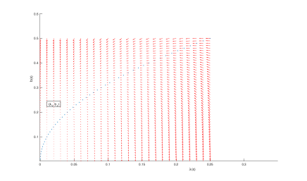
   (a) $\beta>0$

   

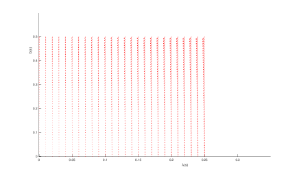
   (b) $\beta<0$

   

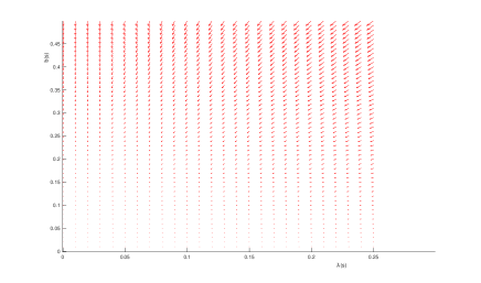
   (c) $\beta=0$

   Figure 1. $(\lambda,b)$ flows driven by the vector fields $(-\lambda b,-b^{2}+\beta\lambda)$ with different $\beta\in\mathbb{R}$.

In order to adjust the value of the energy of $P_{b,\lambda,\gamma}$ in (2.15) up to small error, and to close the bootstrap argument for $(\lambda,b)$ at the end of the proof of Proposition 3.2, we will choose suitable final conditions $\lambda_{1}$ and $b_{1}$ of $(\lambda,b)$ at sufficiently large rescaled time $s_{1}$ as the base case (see (3.5) and (3.11)). Let $E_{0}\in\mathbb{R}$ and

$$C_{0}=\frac{8E_{0}}{\displaystyle\int_{\mathbb{R}}|y|^{2}Q^{2}\,dy}.$$

Fix $0<\lambda_{0}\ll 1$ such that $2\beta+C_{0}\lambda_{0}>0$, and for $\lambda\in(0,\lambda_{0}]$, we define the auxiliary function

$$\mathcal{F}(\lambda)=\int_{\lambda}^{\lambda_{0}}\frac{d\tau}{\tau^{\frac{1}{2}+1}\sqrt{2\beta+C_{0}\tau}}\quad\Longrightarrow\quad\frac{d}{d\lambda}\mathcal{F}(\lambda)=-\frac{1}{\lambda^{\frac{1}{2}+1}\sqrt{2\beta+C_{0}\lambda}},$$ (2.43)

where $\mathcal{F}$ is related to the resolution of $\lambda$ and $b$ for the system (2.39) with $c_{0}=C_{0}$. (See (3.62) and (3.63) in the proof of Proposition 3.12 in Subsection 3.4 for more details.)

Lemma 2.5.

Let $s_{1}\gg 1$, then there exist sufficiently small $\lambda_{1}>0$ and $b_{1}$ such that

$$\left|\frac{\lambda_{1}^{\frac{1}{2}}}{\lambda_{\rm app}^{\frac{1}{2}}(s_{1})}-1\right|+\left|\frac{b_{1}}{b_{\rm app}(s_{1})}-1\right|\lesssim s_{1}^{-1},$$ (2.44)

$$\mathcal{F}(\lambda_{1})=s_{1},\quad\mathcal{E}(b_{1},\lambda_{1})=C_{0}.$$ (2.45)

Proof.

For sufficiently large $s_{1}$, we firstly choose $\lambda_{1}$. By (2.43), $\mathcal{F}$ is a decreasing function of $\lambda$ satisfying $\mathcal{F}(\lambda_{0})=0$ and $\displaystyle\lim_{\lambda\to 0}\mathcal{F}(\lambda)=+\infty$. Thus there exists a unique $\lambda_{1}\in(0,\lambda_{0})$ such that $\mathcal{F}(\lambda_{1})=s_{1}$.

For $\lambda\in(0,\lambda_{0}]$, we have

$$\left|\mathcal{F}(\lambda)-\frac{2}{\sqrt{2\beta}\lambda^{\frac{1}{2}}}\right|\lesssim 1+\left|\int_{\lambda}^{\lambda_{0}}\frac{d\tau}{\tau^{\frac{1}{2}+1}}\left[\frac{1}{\sqrt{2\beta+C_{0}\tau}}-\frac{1}{\sqrt{2\beta}}\right]\right|\lesssim 1.$$ (2.46)

If taking $\lambda=\lambda_{1}$, we obtain from $\mathcal{F}(\lambda_{1})=s_{1}$ and $\lambda_{\rm app}(s)=2/(\beta s^{2})$ that

$$\left|s_{1}-\frac{2}{\sqrt{2\beta}\lambda_{1}^{\frac{1}{2}}}\right|\lesssim 1\quad\Longleftrightarrow\quad\left|\frac{\lambda_{1}^{\frac{1}{2}}}{\lambda_{\rm app}^{\frac{1}{2}}(s_{1})}-1\right|\lesssim s_{1}^{-1}.$$

Secondly, we can choose $b_{1}$ sufficiently small. From the definition of $\mathcal{E}(b,\lambda)$ and $\lambda_{\rm app}(s)=2/(\beta s^{2})$, we define the function $h(b)$ as follows

$$h(b):=\lambda_{1}^{2}\mathcal{E}(b,\lambda_{1}) =b^{2}-\left(\frac{2}{s_{1}}\right)^{2}-2\beta\left(\lambda_{1}-\lambda_{\rm app}(s_{1})\right)+\lambda_{1}\sum_{(j,k)\in\Sigma_{K},\ j+k\geq 1}b^{2j}\lambda_{1}^{k}\eta_{j,k}$$

$$=\big{(}1+O(s^{-2}_{1})\big{)}b^{2}-\left(\frac{2}{s_{1}}\right)^{2}+O(s_{1}^{-3}),$$

where $b$ is close to $b_{\rm app}(s_{1})$. By $b_{\rm app}(s)=2/s$, we have

$$|h(b_{\rm app}(s_{1}))|\lesssim s_{1}^{-3},\quad|h^{\prime}(b_{\rm app}(s_{1}))|\geq 2b_{\rm app}(s_{1})+O(s_{1}^{-3})\geq{s_{1}^{-1}}.$$

Since $C_{0}\lambda_{1}^{2}\approx s_{1}^{-4}$, it follows from the implicit function theorem that there exists a unique $b_{1}$ such that

$$h(b_{1})=C_{0}\lambda_{1}^{2},\quad\text{where}\quad|b_{1}-b_{\rm app}(s_{1})|\lesssim s^{-3}_{1}/s^{-1}_{1}\lesssim s_{1}^{-2},$$

which implies $\mathcal{E}(b_{1},\lambda_{1})=h(b_{1})/\lambda^{2}_{1}=C_{0},$ and completes the proof. ∎

3. Uniform estimates in the rescaled time variable

After the construction of the refined blow-up profile in Proposition 2.1 and final data setup on modulation parameters $\lambda,b$ at the rescaled time $s=s_{1}$ in Lemma 2.5, we will show the uniform backwards estimates of $(\lambda,b,\varepsilon)$ for specific solutions of (1.1) on $[s_{0},s_{1}]$ in Proposition 3.2, where $s_{0}$ is sufficiently large, but independent of $s_{1}$. These uniform backwards estimates will play key role to construct minimal mass blow-up solution of (1.1) by the standard compact argument in next section.

Let $P$, $P_{b}$ be defined by (2.6), (2.10) in Proposition 2.1, $\rho$ be given by (1.15) and define

$$\rho_{b}(s,y):=\rho(y)e^{-i\frac{b(s)|y|^{2}}{4}}.$$ (3.1)

We firstly recall the following standard modulation decomposition of the solution $u(t)$ in the small tube of $Q$.

Lemma 3.1.

There exists $\delta_{0}>0$ small enough such that for any $u(t)\in\mathcal{C}(I,H^{1}(\mathbb{R}))$ satisfying

$$\sup_{t\in I}\inf_{\lambda_{0}>0,\gamma_{0}}\left\|\lambda_{0}^{\frac{1}{2}}u(t,\lambda_{0}y)e^{i\gamma_{0}}-Q(y)\right\|_{H^{1}}\leq\delta_{0},$$ (3.2)

there exist $\mathcal{C}^{1}$ functions $\lambda\in(0,+\infty)$, $b\in\mathbb{R}$, $\gamma\in\mathbb{R}$ on $I$ such that $u$ admits a unique decomposition of the form

$$u(t,x)=\frac{1}{\lambda^{\frac{1}{2}}(t)}\left(P_{b(t)}+\varepsilon(t,y)\right)e^{i\gamma(t)},\qquad y=\frac{x}{\lambda(t)},$$ (3.3)

where the remainder $\varepsilon$ obeys the following orthogonality structure:

$$\forall\ t\in I,\quad\left(\varepsilon,i\Lambda P_{b}\right)_{2}=\left(\varepsilon,|y|^{2}P_{b}\right)_{2}=\left(\varepsilon,i\rho_{b}\right)_{2}=0.$$ (3.4)

Proof.

Please refer to [52] for details. ∎

Let $E_{0}\in\mathbb{R}$ and $t_{1}<0$ be close to $0$. By Remark 2.4, we set up the initial rescaled time $s_{1}$ as

$$s_{1}:=\left|C_{s}^{-1}t_{1}\right|^{-1/3}\gg 1\quad\Longleftrightarrow\quad t_{1}=t_{\rm app}(s_{1}).$$

Let $\lambda_{1}$ and $b_{1}$ be given by Lemma 2.5. Let $u(t)$ be the solution of $\eqref{eq:dnls}$ for $t\leq t_{1}$ with final data

$$u(t_{1},x)=\frac{1}{\lambda_{1}^{\frac{1}{2}}}P_{b_{1}}\left(\frac{x}{\lambda_{1}}\right).$$ (3.5)

As long as the solution $u(t)$ satisfies (3.2), we consider its modulation decomposition $(\lambda,b,\gamma,\varepsilon)$ from Lemma 3.1 and define the rescaled time variable $s$ related to $\lambda$ by

$$s=s_{1}-\int_{t}^{t_{1}}\frac{1}{\lambda^{2}(\tau)}d\tau\quad\Longleftrightarrow\quad\frac{ds}{dt}=\frac{1}{\lambda^{2}(s)}\quad\text{and}\quad s_{1}=s(t_{1}).$$ (3.6)

The main result in this subsection is the following uniform backwards estimates on the decomposition of $u(s)$ on the rescaled time interval $[s_{0},s_{1}]$, where $s_{0}$ is sufficiently large, but independent of $s_{1}$.

Proposition 3.2.

Let $\mu>0$ and $K\geq 7$, there exists sufficiently large $s_{0}>0$, which is independent of $s_{1}$ such that the solution $u$ of $\eqref{eq:dnls}$ with final data (3.5) exists and satisfies (3.2) on the rescaled time interval $[s_{0},s_{1}]$. Moreover, its modulation decomposition

$$u(t,x)=\frac{1}{\lambda^{\frac{1}{2}}(s)}\left(P_{b}+\varepsilon\right)\left(s,y\right)e^{i\gamma(s)},\quad\text{where}\quad\frac{ds}{dt}=\frac{1}{\lambda^{2}(s)},\quad y=\frac{x}{\lambda(s)},$$

satisfies the following uniform estimates

$$\lVert\varepsilon(s)\rVert_{H^{1}}\lesssim s^{-(K+1)},\quad\left|\frac{\lambda^{\frac{1}{2}}(s)}{\lambda_{\rm app}^{\frac{1}{2}}(s)}-1\right|+\left|\frac{b(s)}{b_{\rm app}(s)}-1\right|\lesssim s^{-1}$$ (3.7)

on $[s_{0},s_{1}]$. In addition, we have for any $s\in[s_{0},s_{1}]$ that

$$|E(P_{b,\lambda,\gamma}(s))-E_{0}|\leq O(s^{-K+3}).$$ (3.8)

In the rest of this part, we will use a bootstrap argument involving the following estimates

$$\lVert\varepsilon(s)\rVert_{H^{1}}<s^{-K},\quad\left|\frac{\lambda^{\frac{1}{2}}(s)}{\lambda_{\rm app}^{\frac{1}{2}}(s)}-1\right|+\left|\frac{b(s)}{b_{\rm app}(s)}-1\right|<s^{-\frac{1}{2}}$$ (3.9)

to show (3.7) and complete the proof of Proposition (3.2).

3.1. Bootstrap argument

For $s_{0}>0$ to be chosen large enough (independently of $s_{1}$), we define

$$s_{*}=\inf\{\tau\in[s_{0},s_{1}];\eqref{est:small est:rough}\text{ holds on }[\tau,s_{1}]\}.$$ (3.10)

By (2.44) and (3.5), the base case for the induction argument

$$\varepsilon(s_{1})\equiv 0,\quad\left|\frac{\lambda_{1}^{\frac{1}{2}}}{\lambda_{\rm app}^{\frac{1}{2}}(s_{1})}-1\right|+\left|\frac{b_{1}}{b_{\rm app}(s_{1})}-1\right|\lesssim s_{1}^{-1}<s^{-\frac{1}{2}}_{1}$$ (3.11)

holds for $s_{1}$ large, hence $s_{*}$ is well-defined and $s_{*}<s_{1}$ by the continuity of the solution of (1.1) in $H^{1}(\mathbb{R})$. After the preparations in Subsection 3.2 and Subsection 3.3, we will prove that the estimates (3.7) and (3.8) hold on $[s_{*},s_{1}]$ in Subsection 3.4. Then we obtain $s_{*}=s_{0}$ from the bootstrap argument and complete the proof of Proposition 3.2. Two key ingredients in the proof are the follows:

1. Dynamical estimate of the parameters $(\lambda,b)$ in Subsection 3.2 by deriving the modulation equations from the orthogonal structure of $\varepsilon$ in Lemma 3.1, the mass conservation law and the construction of $P_{b}$ in Proposition 2.1.

2. Dynamical estimate of the remainder $\varepsilon$ in Subsection 3.3 by combining the Energy-Morawetz functional with the coercivity property of the linearized operators $L_{\pm}$. The Energy-Morawetz estimate was firstly used in [61].

3.2. Modulation equations

In this part, we work with the solution $u(t)$ of Proposition 3.2 on the rescaled time interval $[s_{*},s_{1}]$ (i.e. $\varepsilon$ and $\lambda,b$ satisfy (3.9) by the definition of $s_{*}$ in (3.10)), and show the dynamics of the modulation parameters $\lambda,b$, which can be approximated by (2.37) up to small error. Define

$$\operatorname{Mod}(s)=\begin{pmatrix}\frac{\lambda_{s}}{\lambda}+b\\ b_{s}+b^{2}-\theta\\ 1-\gamma_{s}\end{pmatrix}.$$ (3.12)

Lemma 3.3.

For all $s\in[s_{*},s_{1}]$, then we have

$$|\operatorname{Mod}(s)|\lesssim s^{-(K+2)},$$ (3.13)

$$|\left(\varepsilon(s),P_{b}\right)_{2}|<s^{-(K+2)}.$$ (3.14)

Proof.

Since $\varepsilon(s_{1})\equiv 0$, we may define

$$s_{**}=\inf\{s\in[s_{*},s_{1}];\ |\left(\varepsilon(\tau),P_{b}\right)_{2}|<\tau^{-(K+2)}\text{ holds on }[s,s_{1}]\}.$$

Therefore, for any $s\in[s_{**},s_{1}]$, we have

$$|\left(\varepsilon(s),P_{b}\right)_{2}|\leq s^{-(K+2)}.$$ (3.15)

Since the estimates of (3.13) and (3.14) are mixed, we divide the proof into two steps and use the bootstrap argument to conclude the proof.

Step 1: Estimate of the modulation system ${\rm Mod}(s)$ on $[s_{**},s_{1}]$.

By (1.1) and (2.11), $\varepsilon$ should satisfy the following difference equation:

$$i\varepsilon_{s}+\partial^{2}_{y}\varepsilon+ib\Lambda\varepsilon-\varepsilon+\big{(}f(P_{b}+\varepsilon)-f(P_{b})\big{)}+\lambda\,\big{(}g(P_{b}+\varepsilon)-g(P_{b})\big{)}\\ -i\left(\frac{\lambda_{s}}{\lambda}+b\right)\Lambda(P_{b}+\varepsilon)+(1-\gamma_{s})(P_{b}+\varepsilon)+\big{(}b_{s}+b^{2}-\theta\big{)}\frac{|y|^{2}}{4}P_{b}\\ =-\Psi_{K}e^{-i\frac{b|y|^{2}}{4}},$$ (3.16)

where we used the fact that (1.14).

Formally, by combining the equation (3.16) on $\varepsilon$ with the estimate (2.9) on $\Psi_{K}$, we differentiate in time the orthogonality conditions for $\varepsilon$ provided in Lemma 3.1, to obtain the dynamics of the modulation parameters $\lambda,b$ and $\gamma$. Since it is a standard argument (see e.g. [53, 58, 61]), we only sketch the proof here.

As for the orthogonality condition $\left(\varepsilon,i\Lambda P_{b}\right)_{2}=0$.

Taking time derivative on $\left(\varepsilon,i\Lambda P_{b}\right)_{2}=0$, we obtain

$$\left\langle\varepsilon_{s},i\Lambda P_{b}\right\rangle=-\left\langle\varepsilon,i\partial_{s}(\Lambda P_{b})\right\rangle.$$

First, we consider the contribution from the term $\left\langle\varepsilon,i\partial_{s}(\Lambda P_{b})\right\rangle$. By (2.10), we have

$$\Lambda P_{b}=\left(\Lambda P-ib\frac{|y|^{2}}{2}P\right)e^{-ib\frac{|y|^{2}}{4}},$$ (3.17)

and

$$\frac{d}{ds}(\Lambda P_{b})=\left((\Lambda P)_{s}-ib_{s}\frac{|y|^{2}}{4}\Lambda P-ib_{s}\frac{|y|^{2}}{2}P-ib\frac{|y|^{2}}{2}(P)_{s}-bb_{s}\frac{|y|^{4}}{8}P\right)e^{-i\frac{b}{4}|y|^{2}},$$ (3.18)

where we estimate $(P)_{s}$ from (2.6) as follows,

$$(P)_{s}=\frac{\lambda_{s}}{\lambda}\bigg{(}\sum_{(j,k)\in\Sigma_{K}}(k+1)b^{2j}\lambda^{k+1}P_{j,k}^{+}+i\sum_{(j,k)\in\Sigma_{K}}(k+1)b^{2j+1}\lambda^{k+1}P_{j,k}^{-}\Bigg{)}\\ +b_{s}\bigg{(}\sum_{(j,k)\in\Sigma_{K}}2jb^{2j-1}\lambda^{k+1}P_{j,k}^{+}+i\sum_{(j,k)\in\Sigma_{K}}(2j+1)b^{2j}\lambda^{k+1}P_{j,k}^{-}\Bigg{)}\\ =\left(\frac{\lambda_{s}}{\lambda}+b\right)\bigg{(}\sum_{(j,k)\in\Sigma_{K}}(k+1)b^{2j}\lambda^{k+1}P_{j,k}^{+}+i\sum_{(j,k)\in\Sigma_{K}}(k+1)b^{2j+1}\lambda^{k+1}P_{j,k}^{-}\Bigg{)}\\ \qquad+\left(b_{s}+b^{2}-\theta\right)\bigg{(}\sum_{(j,k)\in\Sigma_{K}}2jb^{2j-1}\lambda^{k+1}P_{j,k}^{+}+i\sum_{(j,k)\in\Sigma_{K}}(2j+1)b^{2j}\lambda^{k+1}P_{j,k}^{-}\Bigg{)}\\ -b\bigg{(}\sum_{(j,k)\in\Sigma_{K}}(k+1)b^{2j}\lambda^{k+1}P_{j,k}^{+}+i\sum_{(j,k)\in\Sigma_{K}}(k+1)b^{2j+1}\lambda^{k+1}P_{j,k}^{-}\Bigg{)}\\ -\left(b^{2}-\theta\right)\bigg{(}\sum_{(j,k)\in\Sigma_{K}}2jb^{2j-1}\lambda^{k+1}P_{j,k}^{+}+i\sum_{(j,k)\in\Sigma_{K}}(2j+1)b^{2j}\lambda^{k+1}P_{j,k}^{-}\Bigg{)},$$ (3.19)

and similar estimate about $(\Lambda P)_{s}$. From the properties of the functions $P_{j,k}^{\pm}$ in Proposition 2.1, we can deduce from (3.18) that

$$\sup_{y\in\mathbb{R}}\left(e^{\frac{|y|}{2}}\left|\frac{d}{ds}(\Lambda P_{b})(y)\right|\right)\lesssim|\operatorname{Mod}(s)|+b^{2}(s)+\lambda(s).$$

Thus, by (3.9), we obtain for any $s\in[s_{**},s_{1}]$ that

$$|\left(\varepsilon,i\partial_{s}(\Lambda P_{b})\right)_{2}|\lesssim\|\varepsilon(s)\|_{2}\Big{(}|\operatorname{Mod}(s)|+b^{2}(s)+\lambda(s)\Big{)}\lesssim s^{-2}|\operatorname{Mod}(s)|+s^{-(K+2)}.$$ (3.20)

Next, we deal with the term $\left\langle\varepsilon_{s},i\Lambda P_{b}\right\rangle=-\left\langle i\varepsilon_{s},\Lambda P_{b}\right\rangle$. We firstly estimate the contribution from the first line in (3.16). By (2.10), (3.9), we have

$$\partial^{2}_{y}\varepsilon+ib\Lambda\varepsilon=e^{-ib\frac{|y|^{2}}{4}}\partial^{2}_{y}\left(e^{ib\frac{|y|^{2}}{4}}\varepsilon\right)+b^{2}\frac{|y|^{2}}{4}\varepsilon,$$ (3.21)

$$f(P_{b}+\varepsilon)-f(P_{b})=e^{-ib\frac{|y|^{2}}{4}}\left(f\left(P+e^{ib\frac{|y|^{2}}{4}}\varepsilon\right)-f(P)\right)\\ =e^{-ib\frac{|y|^{2}}{4}}df(P)\left(e^{ib\frac{|y|^{2}}{4}}\varepsilon\right)+O(|\varepsilon|^{2})\\ =e^{-ib\frac{|y|^{2}}{4}}df(P)\left(e^{ib\frac{|y|^{2}}{4}}\varepsilon\right)+O(s^{-2}|\varepsilon|),$$ (3.22)

and

$$\lambda\,\big{(}g(P_{b}+\varepsilon)-g(P_{b})\big{)}=\lambda\mu\delta\varepsilon=O(s^{-2}|\varepsilon(0)|).$$ (3.23)

Therefore, by (3.9), (3.15), and the definition of $P$ in (2.6), we have for any $s\in[s_{**},s_{1}]$ that

$$\left\langle-\partial^{2}_{y}\varepsilon-ib\Lambda\varepsilon+\varepsilon-(f(P_{b}+\varepsilon)-f(P_{b}))-\lambda\left(g(P_{b}+\varepsilon)-g(P_{b})\right),\Lambda P_{b}\right\rangle\\ =\left\langle-\partial^{2}_{y}\left(e^{ib\frac{|y|^{2}}{4}}\varepsilon\right)+e^{ib\frac{|y|^{2}}{4}}\varepsilon-df(Q)\left(e^{ib\frac{|y|^{2}}{4}}\varepsilon\right),\Lambda Q-ib\frac{|y|^{2}}{2}Q\right\rangle+O(s^{-2}\|\varepsilon\|_{H^{1}})\\ =\left\langle L_{+}\left(e^{ib\frac{|y|^{2}}{4}}\varepsilon\right),\Lambda Q\right\rangle-\frac{b}{2}\left\langle L_{-}\left(e^{ib\frac{|y|^{2}}{4}}\varepsilon\right),i|y|^{2}Q\right\rangle+O(s^{-2}\|\varepsilon\|_{H^{1}})\\ =\left\langle e^{ib\frac{|y|^{2}}{4}}\varepsilon,L_{+}(\Lambda Q)\right\rangle-\frac{b}{2}\left\langle e^{ib\frac{|y|^{2}}{4}}\varepsilon,iL_{-}(|y|^{2}Q)\right\rangle+O(s^{-2}\|\varepsilon\|_{H^{1}})\\ =-2\left(\varepsilon,e^{-ib\frac{|y|^{2}}{4}}Q\right)_{2}+2b\left(\varepsilon,ie^{-ib\frac{|y|^{2}}{4}}\Lambda Q\right)_{2}+O(s^{-2}\|\varepsilon\|_{H^{1}})\\ =-2\left(\varepsilon,P_{b}\right)_{2}+2b\left(\varepsilon,i\Lambda P_{b}\right)_{2}+O(s^{-2}\|\varepsilon\|_{H^{1}})=O(s^{-(K+2)}),$$ (3.24)

where in the fourth equality we use the algebraic structure (1.15) of the operators $L_{\pm}$ and in the last equality we use (3.15) and the orthogonal relation $\left(\varepsilon,i\Lambda P_{b}\right)_{2}=0$ in (3.4).

We secondly consider the contribution from the second line in (3.16). By the facts that $\left(P_{b},\Lambda P_{b}\right)_{2}=0$ and

$$\left(|y|^{2}P_{b},\Lambda P_{b}\right)_{2}=-\lVert yP_{b}\rVert^{2}_{2},$$ (3.25)

we have for any $s\in[s_{**},s_{1}]$ that

$$\left(-i\left(\frac{\lambda_{s}}{\lambda}+b\right)\Lambda(P_{b}+\varepsilon)+(1-\gamma_{s})(P_{b}+\varepsilon)+(b_{s}+b^{2}-\theta)\frac{|y|^{2}}{4}P_{b},\Lambda P_{b}\right)_{2}\\ =-\frac{1}{4}\Big{(}b_{s}+b^{2}-\theta\Big{)}\lVert yP_{b}\rVert_{2}^{2}+O(|\operatorname{Mod}(s)|\lVert\varepsilon\rVert_{H^{1}})\\ =-\frac{1}{4}\Big{(}b_{s}+b^{2}-\theta\Big{)}\lVert yQ\rVert_{2}^{2}+O(s^{-2}|\operatorname{Mod}(s)|),$$ (3.26)

where we used (3.9), and the definition of $P_{b}$ in (2.10).

Finally, we consider the contribution from the third line in (3.16). By (2.9), we have

$$\left|\left(\Psi_{K},\Lambda P-ib\frac{|y|^{2}}{2}P\right)_{2}\right|\lesssim s^{-2}|\operatorname{Mod}(s)|+s^{-2(K+2)}.$$ (3.27)

Combining (3.20), (3.24), (3.26) and (3.27), we have for any $s\in[s_{**},s_{1}]$ that

$$|b_{s}+b^{2}-\theta|\lesssim s^{-2}|\operatorname{Mod}(s)|+s^{-(K+2)}.$$ (3.28)

As for the orthogonality condition $\left(\varepsilon,|y|^{2}P_{b}\right)_{2}=0$.

Taking time derivative on $\left(\varepsilon,|y|^{2}P_{b}\right)_{2}=0$, we obtain

$$\left\langle i\varepsilon_{s},i|y|^{2}P_{b}\right\rangle=\left\langle\varepsilon_{s},|y|^{2}P_{b}\right\rangle=-\left\langle\varepsilon,|y|^{2}\partial_{s}(P_{b})\right\rangle.$$

By the definition of $P_{b}$ in (2.10), we have

$$\frac{d}{ds}(P_{b})=\left((P)_{s}-ib_{s}\frac{|y|^{2}}{4}P\right)e^{-i\frac{b}{4}|y|^{2}}.$$ (3.29)

By (3.19) and similar estimate to (3.20), we have for any $s\in[s_{**},s_{1}]$ that

$$|\left(\varepsilon,|y|^{2}\partial_{s}(P_{b})\right)_{2}|\lesssim s^{-2}|\operatorname{Mod}(s)|+s^{-(K+2)}.$$ (3.30)

Next, we consider the term $\left\langle i\varepsilon_{s},i|y|^{2}P_{b}\right\rangle$. Similar to (3.24), we compute by (2.6), (2.10), (3.9) as follows

$$\quad\left\langle-\partial^{2}_{y}\varepsilon-ib\Lambda\varepsilon+\varepsilon-(f(P_{b}+\varepsilon)-f(P_{b}))-\lambda\left(g(P_{b}+\varepsilon)-g(P_{b})\right),i|y|^{2}P_{b}\right\rangle\\ =\left\langle-\partial^{2}_{y}\left(e^{ib\frac{|y|^{2}}{4}}\varepsilon\right)+e^{ib\frac{|y|^{2}}{4}}\varepsilon-df(Q)\left(e^{ib\frac{|y|^{2}}{4}}\varepsilon\right),i|y|^{2}Q\right\rangle+O(s^{-2}\|\varepsilon\|_{H^{1}})\\ =\left\langle L_{-}\left(e^{ib\frac{|y|^{2}}{4}}\varepsilon\right),i|y|^{2}Q\right\rangle+O(s^{-2}\|\varepsilon\|_{H^{1}})\\ =\left\langle e^{ib\frac{|y|^{2}}{4}}\varepsilon,iL_{-}(|y|^{2}Q)\right\rangle+O(s^{-2}\|\varepsilon\|_{H^{1}})\\ =-2\left(\varepsilon,ie^{-ib\frac{|y|^{2}}{4}}\Lambda Q\right)_{2}+O(s^{-2}\|\varepsilon\|_{H^{1}})\\ =-2\left(\varepsilon,ie^{-ib\frac{|y|^{2}}{4}}\Lambda P\right)_{2}+O(s^{-2}\|\varepsilon\|_{H^{1}})\\ =-2\left(\varepsilon,i\Lambda P_{b}\right)_{2}+b\left(\varepsilon,|y|^{2}P_{b}\right)_{2}+O(s^{-2}\|\varepsilon\|_{H^{1}})=O(s^{-(K+2)}),$$ (3.31)

where we used (1.15) in the fourth equality, and the orthogonal relation (3.4) in the last equality. Similar to  (3.26), we have

$$\left(-i\left(\frac{\lambda_{s}}{\lambda}+b\right)\Lambda\big{(}P_{b}+\varepsilon\big{)}+(1-\gamma_{s})\big{(}P_{b}+\varepsilon\big{)}+\big{(}b_{s}+b^{2}-\theta\big{)}\frac{|y|^{2}}{4}P_{b},i|y|^{2}P_{b}\right)_{2}\\ =-\left(\frac{\lambda_{s}}{\lambda}+b\right)\left(\Lambda P_{b},|y|^{2}P_{b}\right)_{2}+O(|\operatorname{Mod}(s)|\lVert\varepsilon\rVert_{H^{1}})\\ =\left(\frac{\lambda_{s}}{\lambda}+b\right)\lVert yQ\rVert_{2}^{2}+O(s^{-2}|\operatorname{Mod}(s)|),$$ (3.32)

where we used (3.25) in the first equality. By (2.9), we have

$$\left|\left(\Psi_{K},i|y|^{2}P\right)_{2}\right|\lesssim s^{-2}|\operatorname{Mod}(s)|+s^{-2(K+2)}.$$ (3.33)

By combining (3.30), (3.31), (3.32) and (3.33), we have for any $s\in[s_{**},s_{1}]$ that

$$\left|\frac{\lambda_{s}}{\lambda}+b\right|\lesssim s^{-2}|\operatorname{Mod}(s)|+s^{-(K+2)}.$$ (3.34)

As for the orthogonality condition $\left(\varepsilon,i\rho_{b}\right)_{2}=0$.

Taking time derivative on $\left(\varepsilon,i\rho_{b}\right)_{2}=0$, we obtain

$$-\left\langle i\varepsilon_{s},\rho_{b}\right\rangle=\left\langle\varepsilon_{s},i\rho_{b}\right\rangle=-\left\langle\varepsilon,\partial_{s}(\rho_{b})\right\rangle.$$

By the definition of $\rho_{b}$ in (3.1), we have

$$\frac{d}{ds}(\rho_{b})=-ib_{s}\frac{|y|^{2}}{4}\rho\ e^{-i\frac{b}{4}|y|^{2}}.$$ (3.35)

By similar estimate as (3.20), we have for any $s\in[s_{**},s_{1}]$ that

$$|\left(\varepsilon,\partial_{s}(\rho_{b})\right)_{2}|\lesssim s^{-2}|\operatorname{Mod}(s)|+s^{-(K+2)}.$$ (3.36)

Next, we consider the term $\left\langle i\varepsilon_{s},\rho_{b}\right\rangle$. Similar to (3.24), we computer by (3.9) as follows

$$\quad\left\langle-\partial^{2}_{y}\varepsilon-ib\Lambda\varepsilon+\varepsilon-(f(P_{b}+\varepsilon)-f(P_{b}))-\lambda\left(g(P_{b}+\varepsilon)-g(P_{b})\right),\rho_{b}\right\rangle$$

$$=\left\langle-\partial^{2}_{y}\left(e^{ib\frac{|y|^{2}}{4}}\varepsilon\right)+e^{ib\frac{|y|^{2}}{4}}\varepsilon-df(Q)\left(e^{ib\frac{|y|^{2}}{4}}\varepsilon\right),\rho\right\rangle+O(s^{-2}\|\varepsilon\|_{H^{1}})$$

$$=\left\langle L_{+}\left(e^{ib\frac{|y|^{2}}{4}}\varepsilon\right),\rho\right\rangle+O(s^{-2}\|\varepsilon\|_{H^{1}})$$

$$=\left\langle e^{ib\frac{|y|^{2}}{4}}\varepsilon,L_{+}\rho\right\rangle+O(s^{-2}\|\varepsilon\|_{H^{1}})$$

$$=\left(\varepsilon,e^{-ib\frac{|y|^{2}}{4}}|y|^{2}Q\right)_{2}+O(s^{-2}\|\varepsilon\|_{H^{1}})$$

$$=\left(\varepsilon,|y|^{2}P_{b}\right)_{2}+O(s^{-2}\|\varepsilon\|_{H^{1}})=O(s^{-(K+2)}),$$ (3.37)

where we used (1.15) in the fourth equality, and the orthogonal relation (3.4) in the last equality. Similar to (3.26), we have

$$\left(-i\left(\frac{\lambda_{s}}{\lambda}+b\right)\Lambda(P_{b}+\varepsilon)+(1-\gamma_{s})(P_{b}+\varepsilon)+(b_{s}+b^{2}-\theta)\frac{|y|^{2}}{4}P_{b},\rho_{b}\right)_{2}\\ =\left(1-\gamma_{s}\right)\left(P_{b},\rho_{b}\right)_{2}+O\left(s^{-2}|\operatorname{Mod}(s)|\right)+O\left(s^{-(K+2)}\right)\\ =\left(1-\gamma_{s}\right)\left(Q,\rho\right)_{2}+O(s^{-2}|\operatorname{Mod}(s)|)+O\left(s^{-(K+2)}\right)\\ =\frac{1}{2}\left(1-\gamma_{s}\right)\lVert yQ\rVert^{2}_{2}+O(s^{-2}|\operatorname{Mod}(s)|)+O\left(s^{-(K+2)}\right),$$ (3.38)

where we used (3.28), (3.34) in the first equality, and (1.16) in the last equality. Last, by (2.9), we have

$$\left|\left(\Psi_{K},\rho\right)_{2}\right|\lesssim s^{-2}|\operatorname{Mod}(s)|+s^{-2(K+2)}.$$ (3.39)

By combining (3.36), (3.37), (3.38) and (3.39), we have for any $s\in[s_{**},s_{1}]$ that

$$\left|1-\gamma_{s}\right|\lesssim s^{-2}|\operatorname{Mod}(s)|+s^{-(K+2)}.$$ (3.40)

By (3.28), (3.34) and (3.40), we obtain that

$$|\operatorname{Mod}(s)|\lesssim s^{-2}|\operatorname{Mod}(s)|+s^{-(K+2)},$$

which implies for any $s\in[s_{**},s_{1}]$ that

$$|\operatorname{Mod}(s)|\lesssim s^{-(K+2)}.$$ (3.41)

Step 2: Estimate of $\left(\varepsilon,P_{b}\right)_{2}$ on $[s_{**},s_{1}]$.

On the one hand, by the mass conservation and (3.5), we have

$$\lVert u(s)\rVert_{2}^{2}=\lVert u(s_{1})\rVert_{2}^{2}=\lVert P_{b}(s_{1})\rVert_{2}^{2}.$$

On the other hand, by the modulation decomposition (3.3), we have

$$\left(\varepsilon(s),P_{b}\right)_{2}=\frac{1}{2}\left(\lVert u(s)\rVert_{2}^{2}-\lVert P_{b}(s)\rVert_{2}^{2}-\lVert\varepsilon(s)\rVert_{2}^{2}\right)=-\frac{1}{2}\lVert\varepsilon(s)\rVert_{2}^{2}+\frac{1}{2}\Big{(}\lVert P_{b}(s_{1})\rVert_{2}^{2}-\lVert P_{b}(s)\rVert_{2}^{2}\Big{)}.$$

Moreover, by (2.13), (3.9) and (3.41), we compute the later as follows

$$\frac{d}{ds}\int_{\mathbb{R}}|P_{b}|^{2}\,dy\lesssim\lambda(s)\left|\rm Mod(s)\right|+s^{-2(K+2)}\lesssim s^{-(K+4)}.$$

By integrating over $[s,s_{1}]$ and combining (3.9), we obtain for any $s\in[s_{**},s_{1}]$ that

$$|\left(\varepsilon(s),P_{b}\right)_{2}|\lesssim s^{-2K}+s^{-(K+3)}\lesssim s^{-(K+3)}.$$

Therefore, we obtain $s_{**}=s_{*}$ for sufficiently large $s_{*}$, and the estimates (3.13) and (3.14) are proved on $[s_{*},s_{1}]$. ∎

Corollary 3.4.

For all $s\in[s_{*},s_{1}]$, then we have

$$|\left(\varepsilon(s),Q\right)_{2}|\lesssim s^{-(K+1)}.$$ (3.42)

Proof.

Note that

$$\left(\varepsilon(s),Q\right)_{2}=\left(\varepsilon(s),P_{b}\right)_{2}-\left(\varepsilon(s),P_{b}-Q\right)_{2}.$$

By (3.9), (3.14) and the fact that $|P_{b}-Q||\lesssim Q^{\frac{1}{2}}\big{(}|b|+\lambda\big{)}\lesssim Q^{\frac{1}{2}}s^{-1}$, we can obtain the result. ∎

3.3. The monotonicity formula: the Energy-Morawetz estimate

After we obtain the dynamics of the modulation parameters in last subsection. Now, we turn to introduce the Energy-Morawetz functional in this subsection, use it in next subsection to improve the estimates about the remainder $\varepsilon$ and modulation parameters $\lambda$, $b$, and then close the bootstrap argument.

The Energy-Morawetz estimate was firstly introduced to construct minimal mass blow-up solution of the inhomogeneous NLS in [61], see also [34, 39, 46, 55]), and recently, it was also successfully applied by B. Dodson to obtain the global well-posedness and scattering results of the defocusing, nonlinear wave equation in the critical Sobolev space $\dot{H}^{s}(\mathbb{R}^{3})$ for $\frac{1}{2}\leq s<1$ in [14, 15].

First, we recall the well-known coercivity property of the linearized operators $L_{\pm}$ around $Q$ in $H^{1}_{\rm rad}(\mathbb{R})$.

Lemma 3.5.

For any $\varepsilon=\varepsilon_{1}+i\varepsilon_{2}\in H^{1}_{\rm rad}(\mathbb{R})$, then there exists constant $C>0$ such that

$$\left\langle L_{+}\varepsilon_{1},\varepsilon_{1}\right\rangle+\left\langle L_{-}\varepsilon_{2},\varepsilon_{2}\right\rangle\geq C\lVert\varepsilon\rVert_{H^{1}}^{2}-\frac{1}{C}\left(\left(\varepsilon_{1},Q\right)_{2}^{2}+\left(\varepsilon_{1},|y|^{2}Q\right)_{2}^{2}+\left(\varepsilon_{2},\rho\right)_{2}^{2}\right).$$

Proof.

Please refer to Lemma $3.2$ in [61] for more details (See also [51, 52, 53, 67]). ∎

Now, we define the linearized energy functional of the remainder $\varepsilon$ according to (3.16) as follows

$$H(s,\varepsilon):=\frac{1}{2}\lVert\partial_{y}\varepsilon\rVert_{2}^{2}+\frac{1}{2}\lVert\varepsilon\rVert_{2}^{2}-\int_{\mathbb{R}}\Big{(}F(P_{b}+\varepsilon)-F(P_{b})-dF(P_{b})\varepsilon\Big{)}dy\\ -\lambda\int_{\mathbb{R}}\Big{(}G(P_{b}+\varepsilon)-G(P_{b})-dG(P_{b})\varepsilon\Big{)}dy.$$

Note that the equation (3.16) can be rewrited as

$$i\varepsilon_{s}-{D_{\varepsilon}}H(s,\varepsilon)+\operatorname{Mod_{op}}(s)P_{b}-i\frac{\lambda_{s}}{\lambda}\Lambda\varepsilon+(1-\gamma_{s})\varepsilon+e^{-ib\frac{|y|^{2}}{4}}\Psi_{K}=0,$$ (3.43)

where $D_{\varepsilon}H(s,\varepsilon)$ denotes the Fréchet derivative of the functional $H(s,\varepsilon)$ with respect to $\varepsilon$ and

$$\operatorname{Mod_{op}}(s)P_{b}=-i\left(\frac{\lambda_{s}}{\lambda}+b\right)\Lambda P_{b}+(1-\gamma_{s})P_{b}+\big{(}b_{s}+b^{2}-\theta\big{)}\frac{|y|^{2}}{4}P_{b}.$$

First, as the consequence of Lemma 3.5, we have the coercivity property for the energy functional $H(s,\varepsilon)$ under the orthogonality conditions of $\varepsilon$ (see (3.4), (3.42)) as follows.

Lemma 3.6.

For all $s\in[s_{*},s_{1}]$, then we have

$$H(s,\varepsilon)\gtrsim\lVert\varepsilon\rVert_{H^{1}}^{2}+O(s^{-2(K+1)}).$$

Proof.

Firstly, from (3.4), (3.9) and (3.42), the following estimates hold:

$$\left(\varepsilon,|y|^{2}Q\right)_{2} =\left(\varepsilon,|y|^{2}P_{b}\right)_{2}+O(|b|\lVert\varepsilon\rVert_{2})+O(\lambda\lVert\varepsilon\rVert_{2})=O(s^{-1}\lVert\varepsilon\rVert_{H^{1}}),$$

$$\left(\varepsilon,i\rho\right)_{2} =\left(\varepsilon,i\rho_{b}\right)_{2}+O(|b|\lVert\varepsilon\rVert_{2})=O(s^{-1}\lVert\varepsilon\rVert_{H^{1}}),$$

$$\left(\varepsilon,Q\right)_{2} =O(s^{-(K+1)}),$$

where we used the fact that $|P_{b}-Q||\lesssim Q^{\frac{1}{2}}\big{(}|b|+\lambda\big{)}$ in the first equality.

Next, If we denote $\varepsilon=\varepsilon_{1}+i\varepsilon_{2}$, then

$$\left|F(P_{b}+\varepsilon)-F(P_{b})-dF(P_{b})\varepsilon-\frac{1}{2}5Q^{4}\varepsilon_{1}^{2}-\frac{1}{2}Q^{4}\varepsilon_{2}^{2}\right|\lesssim e^{-\frac{1}{2}|y|}|\varepsilon|^{3}+|\varepsilon|^{6}+|\varepsilon|^{2}(|b|+\lambda).$$

Thus, from (3.9), we have

$$\left|\int_{\mathbb{R}}\left(F(P_{b}+\varepsilon)-F(P_{b})-dF(P_{b})\varepsilon-\frac{1}{2}5Q^{4}\varepsilon_{1}^{2}-\frac{1}{2}Q^{4}\varepsilon_{2}^{2}\right)\,dy\right|\lesssim O(s^{-1}\lVert\varepsilon\rVert_{H^{1}}^{2}),$$

and

$$\lambda\int_{\mathbb{R}}\Big{(}G(P_{b}+\varepsilon)-G(P_{b})-dG(P_{b})\varepsilon\Big{)}dx=O(s^{-2}\lVert\varepsilon\rVert_{H^{1}}^{2}).$$

Therefore, we have

$$\left|H(s,\varepsilon)-\frac{1}{2}\left\langle L_{+}\varepsilon_{1},\varepsilon_{1}\right\rangle-\frac{1}{2}\left\langle L_{-}\varepsilon_{2},\varepsilon_{2}\right\rangle\right|\lesssim O(s^{-1}\lVert\varepsilon\rVert_{H^{1}}^{2}),$$

which together with the coercivity properties of $L_{\pm}$ in Lemma 3.5 implies the result. ∎

For future reference, we also need the following localized coercivity property.

Lemma 3.7.

There exists $A_{0}>1$ such that for any $A>A_{0}$, we have

$$\frac{1}{2}\int_{\mathbb{R}}\phantom{}\partial^{2}_{y}\phi_{A}\cdot|\partial_{y}\varepsilon|^{2}\,dy+\frac{1}{2}\lVert\varepsilon\rVert_{2}^{2}-\int_{\mathbb{R}}\Big{(}F(P_{b}+\varepsilon)-F(P_{b})-dF(P_{b})\varepsilon\Big{)}\,dy\gtrsim\lVert\varepsilon\rVert^{2}_{2}+O(s^{-2(K+1)}),$$

where the localized function $\phi_{A}$ is defined in Section 1.4,

Proof.

Please refer to [61] for details. ∎

Second, we compute the time variation of the linearized energy $H(s,\varepsilon)$ as follows.

Lemma 3.8.

For all $s\in[s_{*},s_{1}]$, we have

$$\frac{d}{ds}\Big{(}H(s,\varepsilon(s))\Big{)}=\frac{\lambda_{s}}{\lambda}\Big{(}\lVert\partial_{y}\varepsilon\rVert_{2}^{2}-\left\langle f(P_{b}+\varepsilon)-f(P_{b}),\Lambda\varepsilon\right\rangle\Big{)}+O\big{(}s^{-(2K+3)}\big{)}+O(s^{-2}\lVert\varepsilon\rVert_{H^{1}}^{2}).$$ (3.44)

Proof.

We compute the time derivative for $H$ as follows.

$$\frac{d}{ds}\Big{(}H(s,\varepsilon(s))\Big{)}=D_{s}H(s,\varepsilon)+\left\langle D_{\varepsilon}H(s,\varepsilon),\varepsilon_{s}\right\rangle,$$ (3.45)

where $D_{s}H(s,\varepsilon)$ denotes differentiation of the functional $H(s,\varepsilon)$ with respect to $s$. Therefore, we have

$$D_{s}H(s,\varepsilon)= -\int_{\mathbb{R}}(P_{b})_{s}\Big{(}f(P_{b}+\varepsilon)-f(P_{b})-df(P_{b})\varepsilon\Big{)}\,dy-\lambda\int_{\mathbb{R}}(P_{b})_{s}\Big{(}g(P_{b}+\varepsilon)-g(P_{b})-dg(P_{b})\varepsilon\Big{)}\,dy$$

$$-\lambda_{s}\ \int_{\mathbb{R}}\Big{(}G(P_{b}+\varepsilon)-G(P_{b})-dG(P_{b})\varepsilon\Big{)}\,dy.$$

Note that

$$e^{i\frac{b|y|^{2}}{4}}(P_{b})_{s}=P_{s}-ib_{s}\frac{|y|^{2}}{4}P=P_{s}-i\left(b_{s}+b^{2}-\theta\right)\frac{|y|^{2}}{4}P+i\left(b^{2}-\theta\right)\frac{|y|^{2}}{4}P.$$

By (3.9), (3.19) and Lemma 3.13, we obtain

$$|(P_{b})_{s}|\lesssim\Big{(}\big{|}{\rm Mod(s)}\big{|}+b^{2}+\lambda\Big{)}Q^{\frac{1}{2}}\lesssim s^{-2}e^{-\frac{|y|}{2}},$$

and

$$\left|\lambda_{s}\right|=|\lambda|\left|\frac{\lambda_{s}}{\lambda}\right|\lesssim|\lambda|\Big{(}\big{|}{\rm Mod(s)}\big{|}+|b|\Big{)}\lesssim s^{-3}.$$

Thus, we have

$$|D_{s}H(s,\varepsilon)|\lesssim s^{-2}\|\varepsilon\|_{H^{1}}^{2}.$$ (3.46)

Now, we compute $\left\langle D_{\varepsilon}H(s,\varepsilon),\varepsilon_{s}\right\rangle$. By (3.43) and the fact that $\left\langle i{D_{\varepsilon}}H(s,\varepsilon),{D_{\varepsilon}}H(s,\varepsilon)\right\rangle=0$, we have

$$\left\langle{D_{\varepsilon}}H(s,\varepsilon),\varepsilon_{s}\right\rangle=\left\langle{D_{\varepsilon}}H(s,\varepsilon),i\operatorname{Mod_{op}}(s)P_{b}\right\rangle+\frac{\lambda_{s}}{\lambda}\left\langle{D_{\varepsilon}}H(s,\varepsilon),\Lambda\varepsilon\right\rangle\\ +(1-\gamma_{s})\left\langle{D_{\varepsilon}}H(s,\varepsilon),i\varepsilon\right\rangle+\left\langle{D_{\varepsilon}}H(s,\varepsilon),i\Psi_{K}e^{-ib\frac{|y|^{2}}{4}}\right\rangle.$$ (3.47)

By similar estimates as those in (3.21) (3.22), (3.23) and (3.24), we have

$${D_{\varepsilon}}H(s,\varepsilon)=-\partial^{2}_{y}\varepsilon+\varepsilon-\big{(}f(P_{b}+\varepsilon)-f(P_{b})\big{)}-\lambda\big{(}g(P_{b}+\varepsilon)-g(P_{b})\big{)}\\ =e^{-ib\frac{|y|^{2}}{4}}\left(\big{(}-\partial^{2}_{y}+1-df(Q)\big{)}\left(e^{ib\frac{|y|^{2}}{4}}\varepsilon\right)\right)+ib\Lambda\varepsilon+b^{2}\frac{|y|^{2}}{4}\varepsilon+O(s^{-2}|\varepsilon|).$$

Therefore, by the orthogonal relations in (3.4), (3.14) and the similar estimate as in (3.24), we have

$$\left\langle{D_{\varepsilon}}H(s,\varepsilon),\Lambda P_{b}\right\rangle$$

$$= \left\langle\big{(}-\partial^{2}_{y}+1-df(Q)\big{)}\left(e^{ib\frac{|y|^{2}}{4}}\varepsilon\right),\Lambda Q-ib\frac{|y|^{2}}{2}Q\right\rangle+b\left\langle i\Lambda\varepsilon,\Lambda P_{b}\right\rangle+O(s^{-2}\lVert\varepsilon\rVert_{2})$$

$$= -2\left(\varepsilon,P_{b}\right)_{2}+2b\left(\varepsilon,i\Lambda P_{b}\right)_{2}+b\left\langle i\Lambda\varepsilon,\Lambda P_{b}\right\rangle+O(s^{-2}\lVert\varepsilon\rVert_{2})$$

$$= -2\left(\varepsilon,P_{b}\right)_{2}+2b\left(\varepsilon,i\Lambda P_{b}\right)_{2}+O(|b|\lVert\varepsilon\rVert_{H^{1}})+O(s^{-2}\lVert\varepsilon\rVert_{2})=O(s^{-(K+1)}),$$ (3.48)

and

$$\left\langle{D_{\varepsilon}}H(s,\varepsilon),iP_{b}\right\rangle\\ =\left\langle\big{(}-\partial^{2}_{y}+1-df(Q)\big{)}\left(e^{ib\frac{|y|^{2}}{4}}\varepsilon\right),iQ\right\rangle+b\left\langle i\Lambda\varepsilon,iP_{b}\right\rangle+O(s^{-2}\lVert\varepsilon\rVert_{2})\\ =\left\langle L_{-}\left(e^{ib\frac{|y|^{2}}{4}}\varepsilon\right),iQ\right\rangle-b\left\langle\varepsilon,\Lambda P_{b}\right\rangle+O(s^{-2}\lVert\varepsilon\rVert_{2})\\ =O(|b|\lVert\varepsilon\rVert_{2})+O(s^{-2}\lVert\varepsilon\rVert_{2})=O(s^{-(K+1)}),$$ (3.49)

and

$$\left\langle{D_{\varepsilon}}H(s,\varepsilon),i\frac{|y|^{2}}{4}P_{b}\right\rangle\\ =\left\langle\big{(}-\partial^{2}_{y}+1-df(Q)\big{)}\left(e^{ib\frac{|y|^{2}}{4}}\varepsilon\right),i\frac{|y|^{2}}{4}Q\right\rangle+b\left\langle i\Lambda\varepsilon,i\frac{|y|^{2}}{4}P_{b}\right\rangle+O(s^{-2}\lVert\varepsilon\rVert_{2})\\ =\left\langle L_{-}\left(e^{ib\frac{|y|^{2}}{4}}\varepsilon\right),i\frac{|y|^{2}}{4}Q\right\rangle+O(|b|\lVert\varepsilon\rVert_{2})+O(s^{-2}\lVert\varepsilon\rVert_{2})\\ =-\left(\varepsilon,i\Lambda P_{b}\right)_{2}+O(s^{-1}\lVert\varepsilon\rVert_{2})=O(s^{-(K+1)}).$$ (3.50)

By combining (3.48), (3.49), (3.50) with Lemma 3.3, we obtain

$$\left\langle{D_{\varepsilon}}H(s,\varepsilon),i\operatorname{Mod_{op}}(s)P_{b}\right\rangle=O(s^{-(2K+3)}).$$ (3.51)

Next, we have

$$\left\langle{D_{\varepsilon}}H(s,\varepsilon),\Lambda\varepsilon\right\rangle=\left\langle-\partial^{2}_{y}\varepsilon+\varepsilon-\Big{(}f(P_{b}+\varepsilon)-f(P_{b})\Big{)}-\lambda\Big{(}g(P_{b}+\varepsilon)-g(P_{b})\Big{)},\Lambda\varepsilon\right\rangle.$$ (3.52)

By (3.9) and simple computations, we have

$$\left\langle-\partial^{2}_{y}\varepsilon,\Lambda\varepsilon\right\rangle=\lVert\partial_{y}\varepsilon\rVert_{2}^{2},\quad\left\langle\varepsilon,\Lambda\varepsilon\right\rangle=0,$$

and

$$\left|\left\langle\lambda\big{(}g(P_{b}+\varepsilon)-g(P_{b})\big{)},\Lambda\varepsilon\right\rangle\right|\lesssim O(s^{-2}\lVert\varepsilon\rVert^{2}_{H^{1}}).$$

Thus,

$$\frac{\lambda_{s}}{\lambda}\left\langle{D_{\varepsilon}}H(s,\varepsilon),\Lambda\varepsilon\right\rangle=\frac{\lambda_{s}}{\lambda}\Big{(}\lVert\partial_{y}\varepsilon\rVert_{2}^{2}-\left\langle f(P_{b}+\varepsilon)-f(P_{b}),\Lambda\varepsilon\right\rangle\Big{)}+O\big{(}s^{-3}\|\varepsilon\|_{H^{1}}^{2}\big{)}.$$ (3.53)

For the third term in the right-hand side of (3.47), we have

$$|(1-\gamma_{s})\left\langle{D_{\varepsilon}}H(s,\varepsilon),i\varepsilon\right\rangle|=\Big{|}(1-\gamma_{s})\left\langle\Big{(}f(P_{b}+\varepsilon)-f(P_{b})\Big{)}+\lambda\Big{(}g(P_{b}+\varepsilon)-g(P_{b})\Big{)},\varepsilon\right\rangle\Big{|}\\ \lesssim|\operatorname{Mod}(s)|\Big{(}\lVert\varepsilon\rVert_{2}^{2}+\lVert\varepsilon\rVert_{H^{1}}^{6}\Big{)}=O(s^{-4}\lVert\varepsilon\rVert_{H^{1}}^{2}).$$ (3.54)

Finally, by (2.9) , (3.9) and Lemma 3.3, the fourth term in the right-hand side of (3.47) is estimated by

$$\left|\left\langle{D_{\varepsilon}}H(s,\varepsilon),i\Psi_{K}e^{-ib\frac{|y|^{2}}{4}}\right\rangle\right|\lesssim\left(\lVert\varepsilon\rVert_{H^{1}}+\lVert\varepsilon\rVert_{H^{1}}^{5}\right)\Big{(}\lambda\big{|}{\rm Mod(s)}\big{|}+(b^{2}+\lambda)^{K+2}\Big{)}\\ \leq O(s^{-(K+4)}\lVert\varepsilon\rVert_{H^{1}})\leq O(s^{-(2K+3)})+O(s^{-5}\lVert\varepsilon\rVert_{H^{1}}^{2}).$$ (3.55)

By (3.45), (3.46), (3.47), (3.51), (3.52), (3.53), (3.54) and (3.55), we can complete the proof of Lemma. ∎

Note that as in [61], the time derivative of the linearized energy functional $H(s,\varepsilon)$ in (3.44) cannot be well controlled because of the lack of the good estimate about the additional term $\left\langle f(P_{b}+\varepsilon)-f(P_{b}),\Lambda\varepsilon\right\rangle$, and we need introduce a Morawetz type functional such as

$$\frac{1}{2}\,\mathrm{Im}\int_{\mathbb{R}}\partial_{y}\left(\frac{|y|^{2}}{2}\right)\partial_{y}\varepsilon\bar{\varepsilon}\,dy$$

in $H(s,\varepsilon)$ to cancel the effect from $\left\langle f(P_{b}+\varepsilon)-f(P_{b}),\Lambda\varepsilon\right\rangle$. In fact, we need use a localized function to replace $|y|^{2}/2$ due to the lack of control on $\lVert y\varepsilon\rVert_{2}$.

From now on, we choose $A>A_{0}$ for sufficiently large $A_{0}$. We define the localized Morawetz functional $J(\varepsilon)$ by

$$J(\varepsilon)=\frac{1}{2}\,\mathrm{Im}\int_{\mathbb{R}}\partial_{y}\phi_{A}(y)\cdot\partial_{y}\varepsilon\,\bar{\varepsilon}\,dy,$$

where the localized function $\phi_{A}$ is defined in Section 1.4, and denote the Energy-Morawetz functional $S(s,\varepsilon)$ by

$$S(s,\varepsilon)=\frac{1}{\lambda^{4}(s)}\Big{(}H(s,\varepsilon(s))+b(s)\cdot J(\varepsilon(s))\Big{)}.$$

First, we have

Proposition 3.9.

For any $s\in[s_{*},s_{1}]$, then we have

$$S(s,\varepsilon(s))\gtrsim\frac{1}{\lambda^{4}(s)}\left(\lVert\varepsilon(s)\rVert_{H^{1}}^{2}+O(s^{-2(K+1)}\right).$$

Proof.

By (3.9), we have

$$\big{|}b\cdot J(\varepsilon)\big{|}\leq|b|\lVert\partial_{y}\phi_{A}\rVert_{\infty}\lVert\varepsilon\rVert^{2}_{H^{1}}\lesssim O(s^{-1}\lVert\varepsilon\rVert_{H^{1}}^{2}),$$

which together with Lemma 3.6 implies the result. ∎

Before we compute the time derivative of functional $S(s,\varepsilon)$, we deal with the time derivative of functional $J(\varepsilon)$.

Lemma 3.10.

For all $s\in[s_{*},s_{1}]$, then we have

$$\frac{d}{ds}[J(\varepsilon(s))]=\int_{\mathbb{R}}\phantom{}\partial^{2}_{y}\phi_{A}\cdot|\partial_{y}\varepsilon|^{2}\,dy-\frac{1}{4}\int_{\mathbb{R}}\partial^{4}_{y}\phi_{A}|\varepsilon|^{2}\,dy\\ -\left\langle f(P_{b}+\varepsilon)-f(P_{b}),\frac{1}{2}\partial^{2}_{y}\phi_{A}\varepsilon+\partial_{y}\phi_{A}\partial_{y}\varepsilon\right\rangle+O(s^{-(2K+2)})+O(s^{-1}\lVert\varepsilon\rVert_{H^{1}}^{2}).$$

Note that the term $\left\langle f(P_{b}+\varepsilon)-f(P_{b}),\frac{1}{2}\partial^{2}_{y}\phi_{A}\varepsilon+\partial_{y}\phi_{A}\partial_{y}\varepsilon\right\rangle$ in the above equality is the localized version of $\left\langle f(P_{b}+\varepsilon)-f(P_{b}),\Lambda\varepsilon\right\rangle$ in the right hand side of (3.44).

Proof.

By integration by parts, we have

$$\frac{d}{ds}[J(\varepsilon(s))]=\mathrm{Re}\int_{\mathbb{R}}i\varepsilon_{s}\left(\frac{1}{2}\partial^{2}_{y}\phi_{A}\bar{\varepsilon}+\partial_{y}\phi_{A}\partial_{y}\bar{\varepsilon}\right)\,dy.$$

By (3.9), we estimate the term from the first line of (3.16) as follows.

$$\mathrm{Re}\int_{\mathbb{R}}-\partial^{2}_{y}\varepsilon\left(\frac{1}{2}\partial^{2}_{y}\phi_{A}\bar{\varepsilon}+\partial_{y}\phi_{A}\partial_{y}\bar{\varepsilon}\right)dy=\int_{\mathbb{R}^{d}}\phantom{}\partial^{2}_{y}\phi_{A}|\partial_{y}\varepsilon|^{2}\,dy-\frac{1}{4}\int_{\mathbb{R}}\partial^{4}_{y}\phi_{A}|\varepsilon|^{2}\,dy,$$

$$\mathrm{Re}\int_{\mathbb{R}}\varepsilon\left(\frac{1}{2}\partial^{2}_{y}\phi_{A}\bar{\varepsilon}+\partial_{y}\phi_{A}\partial_{y}\bar{\varepsilon}\right)dy=0,$$

$$b\cdot\mathrm{Re}\int_{\mathbb{R}}i\Lambda\varepsilon\left(\frac{1}{2}\partial^{2}_{y}\phi_{A}\bar{\varepsilon}+\partial_{y}\phi_{A}\partial_{y}\bar{\varepsilon}\right)dy=O\left(|b|\lVert\varepsilon\rVert^{2}_{H^{1}}\right)=O\left(s^{-1}\lVert\varepsilon\rVert^{2}_{H^{1}}\right),$$

and

$$\lambda\cdot\mathrm{Re}\int_{\mathbb{R}}\Big{(}g(P_{b}+\varepsilon)-g(P_{b})\Big{)}\left(\frac{1}{2}\partial^{2}_{y}\phi_{A}\bar{\varepsilon}+\partial_{y}\phi_{A}\partial_{y}\bar{\varepsilon}\right)dy=O(\lambda\lVert\varepsilon\rVert_{H^{1}}^{2})=O(s^{-(2K+2)}).$$

For the term from the second line of (3.16), we obtain from (3.9) and Lemma 3.3 that

$$\left|\left\langle i\left(\frac{\lambda_{s}}{\lambda}+b\right)\Lambda(P_{b}+\varepsilon)-(1-\gamma_{s})(P_{b}+\varepsilon)-(b_{s}+b^{2}-\theta)\frac{|y|^{2}}{4}P_{b},\frac{1}{2}\partial^{2}_{y}\phi_{A}\varepsilon+\partial_{y}\phi_{A}\partial_{y}\varepsilon\right\rangle\right|\\ \lesssim|\operatorname{Mod}(s)|\lVert\varepsilon\rVert_{H^{1}}\lesssim O(s^{-(2K+2)}).$$

Finally, by (2.9) and Lemma 3.3, we have

$$\left|\left\langle\Psi_{K}e^{-i\frac{b|y|^{2}}{4}},\frac{1}{2}\partial^{2}_{y}\phi_{A}\bar{\varepsilon}+\partial_{y}\phi_{A}\partial_{y}\bar{\varepsilon}\right\rangle\right|\\ \lesssim\Big{(}\lambda\big{|}{\rm Mod(s)}\big{|}+(b^{2}+\lambda)^{K+2}\Big{)}\lVert\varepsilon\rVert_{H^{1}}\\ \leq O(s^{-(K+4)}\lVert\varepsilon\rVert_{H^{1}})\leq O(s^{-(2K+4)}).$$

Together with the above estimates, we can obtain the result. ∎

Proposition 3.11.

For any $s\in[s_{*},s_{1}]$, we have

$$\frac{d}{ds}\Big{(}S(s,\varepsilon(s))\Big{)}\gtrsim\frac{b}{\lambda^{4}(s)}\left(\lVert\varepsilon(s)\rVert_{H^{1}}^{2}+O\big{(}s^{-2(K+1)}\big{)}\right).$$

Proof.

By the definition of $S$, we have

$$\frac{d}{ds}\Big{(}S(s,\varepsilon(s))\Big{)}=\frac{1}{\lambda^{4}}\left(-4\frac{\lambda_{s}}{\lambda}\big{(}H(s,\varepsilon)+b\cdot J(\varepsilon)\big{)}+\frac{d}{ds}\big{(}H(s,\varepsilon(s))\big{)}+b\cdot\frac{d}{ds}\big{(}J(\varepsilon(s))\big{)}+b_{s}\cdot J(\varepsilon)\right).$$

First, we claim the following estimate

$$\frac{d}{ds}\big{(}H(s,\varepsilon(s))\big{)}+b\cdot\frac{d}{ds}\big{(}J(\varepsilon(s))\big{)}=-b\lVert\partial_{y}\varepsilon\rVert_{2}^{2}+b\int_{\mathbb{R}}\partial^{2}_{y}\phi_{A}|\partial_{y}\varepsilon|^{2}\,dy+O\left(\frac{b}{A}\lVert\varepsilon\rVert_{H^{1}}^{2}\right)+O(s^{-(2K+3)}).$$ (3.56)

Indeed, by integration by parts, we have

$$-\mathrm{Re}\int_{\mathbb{R}}\Big{(}f(P_{b}+\varepsilon)-f(P_{b})\Big{)}\cdot\Lambda\bar{\varepsilon}\,dy\\ =-\frac{1}{2}\mathrm{Re}\int_{\mathbb{R}}\Big{(}f(P_{b}+\varepsilon)-f(P_{b})\Big{)}\bar{\varepsilon}\,dy-\mathrm{Re}\int_{\mathbb{R}}y\partial_{y}\Big{(}F(P_{b}+\varepsilon)-F(P_{b})-dF(P_{b})\varepsilon\Big{)}\,dy\\ +\mathrm{Re}\int_{\mathbb{R}}\Big{(}f(P_{b}+\varepsilon)-f(P_{b})-df(P_{b})\varepsilon\Big{)}y\partial_{y}\bar{P}_{b}\,dy\\ =-\frac{1}{2}\mathrm{Re}\int_{\mathbb{R}}\Big{(}f(P_{b}+\varepsilon)-f(P_{b})\Big{)}\bar{\varepsilon}\,dy+\mathrm{Re}\int_{\mathbb{R}}\Big{(}F(P_{b}+\varepsilon)-F(P_{b})-dF(P_{b})\varepsilon\Big{)}\,dy\\ +\mathrm{Re}\int_{\mathbb{R}}\Big{(}f(P_{b}+\varepsilon)-f(P_{b})-df(P_{b})\varepsilon\Big{)}y\partial_{y}\bar{P}_{b}\,dy,$$

and

$$-\mathrm{Re}\int_{\mathbb{R}}\Big{(}f(P_{b}+\varepsilon)-f(P_{b})\Big{)}\cdot\left(\frac{1}{2}\partial^{2}_{y}\phi_{A}\bar{\varepsilon}+\partial_{y}\phi_{A}\partial_{y}\bar{\varepsilon}\right)\,dy\\ =-\frac{1}{2}\mathrm{Re}\int_{\mathbb{R}}\Big{(}f(P_{b}+\varepsilon)-f(P_{b})\Big{)}\partial^{2}_{y}\phi_{A}\bar{\varepsilon}\,dy+\mathrm{Re}\int_{\mathbb{R}}\partial^{2}_{y}\phi_{A}\Big{(}F(P_{b}+\varepsilon)-F(P_{b})-dF(P_{b})\varepsilon\Big{)}\,dy\\ +\mathrm{Re}\int_{\mathbb{R}}\Big{(}f(P_{b}+\varepsilon)-f(P_{b})-df(P_{b})\varepsilon\Big{)}\partial_{y}\phi_{A}\partial_{y}\bar{P}_{b}\,dy.$$

Therefore, by combining Lemma 3.8 and Lemma 3.10, we have

$$\frac{d}{ds}\Big{(}H(s,\varepsilon(s))\Big{)}+ b\cdot\frac{d}{ds}\Big{(}J(\varepsilon(s))\Big{)}$$

$$= -b\lVert\partial_{y}\varepsilon\rVert_{2}^{2}+b\int_{\mathbb{R}}\partial^{2}_{y}\phi_{A}|\partial_{y}\varepsilon|^{2}\,dy$$

$$+\left(\frac{\lambda_{s}}{\lambda}+b\right)\cdot\Bigg{(}\lVert\partial_{y}\varepsilon\rVert_{2}^{2}-\frac{1}{2}\,\mathrm{Re}\int_{\mathbb{R}}\Big{(}f(P_{b}+\varepsilon)-f(P_{b})\Big{)}\bar{\varepsilon}\,dy$$

$$\qquad\qquad\qquad+\mathrm{Re}\int_{\mathbb{R}}\Big{(}F(P_{b}+\varepsilon)-F(P_{b})-dF(P_{b})\varepsilon\Big{)}\,dy$$

$$\qquad\qquad\qquad+\mathrm{Re}\int_{\mathbb{R}}\Big{(}f(P_{b}+\varepsilon)-f(P_{b})-df(P_{b})\varepsilon\Big{)}y\partial_{y}\bar{P}_{b}\,dy\Bigg{)}$$

$$\qquad+b\cdot\Bigg{(}-\frac{1}{2}\,\mathrm{Re}\int_{\mathbb{R}}\Big{(}f(P_{b}+\varepsilon)-f(P_{b})\Big{)}\left(\partial^{2}_{y}\phi_{A}-1\right)\bar{\varepsilon}\,dy$$

$$\qquad\qquad\quad+\mathrm{Re}\int_{\mathbb{R}}\Big{(}F(P_{b}+\varepsilon)-F(P_{b})-dF(P_{b})\varepsilon\Big{)}\left(\partial^{2}_{y}\phi_{A}-1\right)\,dy$$

$$\qquad\qquad\quad+\mathrm{Re}\int_{\mathbb{R}}\Big{(}f(P_{b}+\varepsilon)-f(P_{b})-df(P_{b})\varepsilon\Big{)}\left(\partial_{y}\phi_{A}-y\right)\partial_{y}\bar{P}_{b}\,dy\Bigg{)}$$

$$\qquad\qquad\qquad\qquad-\frac{1}{4}\,b\int_{\mathbb{R}}|\varepsilon|^{2}\partial^{4}_{y}\phi_{A}\,dy+O(s^{-(2K+3)})+O(s^{-2}\lVert\varepsilon\rVert_{H^{1}}^{2}).$$

By Lemma 3.3, we have

$$\left|\frac{\lambda_{s}}{\lambda}+b\right|\lesssim\left|{\rm Mod(s)}\right|\lesssim O(s^{-(K+2)}),$$

which together with (3.9) implies that

$$\left|\left(\frac{\lambda_{s}}{\lambda}+b\right)\Bigg{(}\lVert\partial_{y}\varepsilon\rVert_{2}^{2}-\frac{1}{2}\mathrm{Re}\int_{\mathbb{R}}\Big{(}f(P_{b}+\varepsilon)-f(P_{b})\Big{)}\bar{\varepsilon}\,dy+\mathrm{Re}\int_{\mathbb{R}}\Big{(}F(P_{b}+\varepsilon)-F(P_{b})-dF(P_{b})\varepsilon\Big{)}\,dy\right.$$

$$\left.+\mathrm{Re}\int_{\mathbb{R}}\Big{(}f(P_{b}+\varepsilon)-f(P_{b})-df(P_{b})\varepsilon\Big{)}y\partial_{y}\bar{P}_{b}\,dy\Bigg{)}\right|\lesssim s^{-(K+2)}\|\varepsilon\|_{H^{1}}^{2}\lesssim s^{-(3K+2)}.$$

Next, by (3.9) and the exponential decay of $P$, we have

$$|b|\left|-\frac{1}{2}\mathrm{Re}\int_{\mathbb{R}}\Big{(}f(P_{b}+\varepsilon)-f(P_{b})\Big{)}\left(\partial^{2}_{y}\phi_{A}-1\right)\bar{\varepsilon}\,dy\right|\\ \lesssim|b|\int_{\mathbb{R}}\Big{(}|P|^{4}|\partial^{2}_{y}\phi_{A}-1||\varepsilon|^{2}+|\varepsilon|^{6}\Big{)}\,dy\lesssim|b|\cdot e^{-\frac{A}{2}}\lVert\varepsilon\rVert_{2}^{2}+O\left(s^{-1}\lVert\varepsilon\rVert_{H^{1}}^{6}\right),$$

and similarly for

$$b\cdot\mathrm{Re}\int_{\mathbb{R}}\Big{(}F(P_{b}+\varepsilon)-F(P_{b})-dF(P_{b})\varepsilon\Big{)}\left(\partial^{2}_{y}\phi_{A}-1\right)\,dy,$$

and

$$b\cdot\mathrm{Re}\int_{\mathbb{R}}\Big{(}f(P_{b}+\varepsilon)-f(P_{b})-df(P_{b})\varepsilon\Big{)}\left(\partial_{y}\phi_{A}-y\right)\partial_{y}\bar{P}_{b}\,dy.$$

In addition, by the definition of $\phi_{A}$, we have

$$\left|-b\int_{\mathbb{R}}|\varepsilon|^{2}\partial^{4}_{y}\phi_{A}dy\right|\lesssim\frac{|b|}{A^{2}}\lVert\varepsilon\rVert_{2}^{2}.$$

Therefore, we can obtain (3.56).

By Lemma 3.3, we have $-\frac{\lambda_{s}}{\lambda}=b+O(s^{-(K+2)})$, thus we have

$$\quad-4\frac{\lambda_{s}}{\lambda}H(s,\varepsilon)+\frac{d}{ds}\Big{(}H(s,\varepsilon(s))\Big{)}+b\cdot\frac{d}{ds}\Big{(}J(\varepsilon(s))\Big{)}$$

$$\gtrsim 4bH(s,\varepsilon)-b\lVert\partial_{y}\varepsilon\rVert_{2}^{2}+b\int_{\mathbb{R}}\partial^{2}_{y}\phi_{A}|\partial_{y}\varepsilon|^{2}dy+O(s^{-2}\|\varepsilon\|_{H^{1}}^{2})+\frac{b}{A}O(\lVert\varepsilon\rVert_{H^{1}}^{2})+O(s^{-(2K+3)})$$

$$\gtrsim b\left(\int_{\mathbb{R}}\phantom{}\partial^{2}_{y}\phi_{A}|\partial_{y}\varepsilon|^{2}\,dy+\lVert\varepsilon\rVert_{2}^{2}-2\int_{\mathbb{R}}\Big{(}F(P_{b}+\varepsilon)-F(P_{b})-dF(P_{b})\varepsilon\Big{)}\,dy\right)$$

$$\qquad+2bH(s,\varepsilon)+O\left(\frac{b}{A}\lVert\varepsilon\rVert_{H^{1}}^{2}\right)+O(s^{-(2K+3)}).$$

Thus, by choosing $A$ large enough, we can obtain from Lemma 3.6 and Lemma 3.7 that

$$-4\frac{\lambda_{s}}{\lambda}H(s,\varepsilon)+\frac{d}{ds}\Big{(}H(s,\varepsilon(s))\Big{)}+b\cdot\frac{d}{ds}\Big{(}J(\varepsilon(s))\Big{)}\gtrsim b\|\varepsilon\|_{H^{1}}^{2}+O(s^{-(2K+3)}).$$

Finally, by the facts that $b=O(s^{-1})$, $b_{s}=O(s^{-2})$ and $J(\varepsilon)=O(\lVert\varepsilon\rVert_{H^{1}}^{2})$, we have

$$\left(\left|\frac{\lambda_{s}}{\lambda}\right|b+|b_{s}|\right)|J(\varepsilon)|\lesssim s^{-2}\|\varepsilon\|_{H^{1}}^{2},$$

therefore, we have

$$\frac{d}{ds}\Big{(}S(s,\varepsilon(s))\Big{)}\gtrsim\frac{b}{\lambda^{4}}\left(\lVert\varepsilon\rVert_{H^{1}}^{2}+O(s^{-(2K+2)})\right).$$

This completes the proof. ∎

3.4. End of the proof of Proposition 3.2

In this subsection, we finish the proof of Proposition 3.2. Recall from Subsection 3.1 that our goal is to prove $s_{*}=s_{0}$ by improving (3.9) into (3.7). Therefore, it suffices to prove the following result.

Proposition 3.12.

Let $K\geq 7$, then for all $s\in[s_{*},s_{1}]$ , we have

$$\lVert\varepsilon(s)\rVert_{H^{1}}\lesssim s^{-(K+1)},$$ (3.57)

$$\left|\frac{\lambda^{\frac{1}{2}}(s)}{\lambda_{\rm app}^{\frac{1}{2}}(s)}-1\right|+\left|\frac{b(s)}{b_{\rm app}(s)}-1\right|\lesssim s^{-1}.$$ (3.58)

Proof.

First, we prove (3.57). From Proposition 3.9, there exists a constant $\kappa>1$ such that for any $s\in[s_{*},s_{1}]$, we have

$$\frac{1}{\kappa}\frac{1}{\lambda^{4}}\left(\lVert\varepsilon\rVert_{H^{1}}^{2}-\kappa^{2}s^{-2(K+1)}\right)\leq S(s,\varepsilon)\leq\frac{\kappa}{\lambda^{4}}\lVert\varepsilon\rVert_{H^{1}}^{2}.$$ (3.59)

By Proposition 3.11, taking a larger $\kappa$ if necessary, we have

$$\frac{d}{ds}[S(s,\varepsilon(s))]\geq\frac{1}{\kappa}\frac{b}{\lambda^{4}}\left(\lVert\varepsilon\rVert_{H^{1}}^{2}-\kappa^{2}s^{-2(K+1)}\right).$$ (3.60)

Define

$$s_{\dagger}:=\inf\{s\in[s_{*},s_{1}],\quad\lVert\varepsilon(\tau)\rVert_{H^{1}}\leq 2\kappa^{2}\tau^{-(K+1)}\quad\text{for all }\tau\in[s,s_{1}]\}.$$

Since $\varepsilon(s_{1})\equiv 0$, $s_{\dagger}$ is well-defined and $s_{\dagger}<s_{1}$ by the continuity of the solution of (1.1) in $H^{1}(\mathbb{R})$. We argue by contradiction. Assume that $s_{\dagger}>s_{*}$. In particular, we have

$$\lVert\varepsilon(s_{\dagger})\rVert_{H^{1}}=2\kappa^{2}s_{\dagger}^{-(K+1)}.$$

Define

$$s_{\ddagger}:=\sup\{s\in[s_{\dagger},s_{1}],\quad\lVert\varepsilon(\tau)\rVert_{H^{1}}\geq\kappa\tau^{-(K+1)}\quad\text{for all }\tau\in[s_{\dagger},s]\}.$$

In particular, we have $s_{\dagger}<s_{\ddagger}<s_{1}$ and

$$\lVert\varepsilon(s_{\ddagger})\rVert_{H^{1}}=\kappa s_{\ddagger}^{-(K+1)}.$$

From (3.60), $S$ is nondecreasing on $[s_{\dagger},s_{\ddagger}]$. By (3.9), (3.59) and (3.60), we have for $K\geq 7$ that

$$\lVert\varepsilon(s_{\dagger})\rVert_{H^{1}}^{2}-\kappa^{2}s_{\dagger}^{-2(K+1)}\leq\kappa\lambda^{4}(s_{\dagger})S(s_{\dagger},\varepsilon(s_{\dagger}))\leq\kappa\lambda^{4}(s_{\dagger})S(s_{\ddagger},\varepsilon(s_{\ddagger}))\\ \leq\kappa^{2}\frac{\lambda^{4}(s_{\dagger})}{\lambda^{4}(s_{\ddagger})}\|\varepsilon(s_{\ddagger})\|_{H^{1}}^{2}\leq\kappa^{4}\frac{\lambda^{4}(s_{\dagger})}{\lambda^{4}(s_{\ddagger})}s_{\ddagger}^{-2(K+1)}\leq 2\kappa^{4}\left(\frac{s_{\ddagger}}{s_{\dagger}}\right)^{8}s_{\ddagger}^{-2(K+1)}\leq 2\kappa^{4}s_{\dagger}^{-2(K+1)},$$

Therefore, we obtain $\lVert\varepsilon(s_{\dagger})\rVert_{H^{1}}^{2}\leq 3\kappa^{4}s_{\dagger}^{-2(K+1)}$, which is a contradiction with the definition of $s_{\dagger}$. Hence we obtain $s_{\dagger}=s_{*}$ and (3.57) is proved.

Now, we prove (3.58). Recall that $\lambda(s_{1})=\lambda_{1}$ and $b(s_{1})=b_{1}$ are chosen in Lemma 2.5 so that $\mathcal{F}(\lambda(s_{1}))=s_{1}$ and $\displaystyle\mathcal{E}(b(s_{1}),\lambda(s_{1}))=\frac{8E_{0}}{\lVert yQ\rVert^{2}_{L^{2}}}.$ In particular, we deduce from (2.15) that

$$|E(P_{b_{1},\lambda_{1},\gamma_{1}})-E_{0}|\lesssim\frac{(b_{1}^{2}+\lambda_{1})^{K+2}}{\lambda_{1}^{2}}\lesssim s_{1}^{-2K}.$$

By (2.14), (3.9), and (3.13), we have for all $s\in[s_{*},s_{1}]$ that

$$\left|\frac{d}{ds}E(P_{b,\lambda,\gamma})\right|\lesssim\frac{1}{\lambda^{2}}\Big{(}\big{|}{\rm Mod(s)}\big{|}+\big{(}b^{2}+\lambda\big{)}^{K+2}\Big{)}\lesssim s^{-K+2}.$$

In particular, by integration over $[s,s_{1}]$, we obtain that

$$|E(P_{b,\lambda,\gamma}(s))-E_{0}|\lesssim|E(P_{b,\lambda,\gamma}(s))-E(P_{b_{1},\lambda_{1},\gamma_{1}})|+|E(P_{b_{1},\lambda_{1},\gamma_{1}})-E_{0}|\lesssim s^{-K+3}.$$ (3.61)

By (2.15) and (3.9), we have for $K\geq 7$ that

$$\left|\mathcal{E}(b(s),\lambda(s))-\frac{8E_{0}}{\displaystyle\int_{\mathbb{R}}|y|^{2}Q^{2}\,dy}\right|\lesssim s^{-K+3}+O\left(\frac{(b^{2}+\lambda)^{K+2}}{\lambda^{2}}\right)\lesssim s^{-4}.$$

By the expression (2.16) of $\mathcal{E}$ with $\displaystyle C_{0}=\frac{8E_{0}}{\int_{\mathbb{R}}|y|^{2}Q^{2}\,dy}$, we have

$$\left|b^{2}-2\beta\lambda-C_{0}\lambda^{2}\right|\lesssim\lambda(b^{2}+\lambda)+\frac{\lambda^{2}}{s^{4}}\lesssim\frac{\lambda}{s^{2}},$$

where the term $\lambda(b^{2}+\lambda)$ comes from the higher order terms in the definition of $\mathcal{E}(b(s),\lambda(s))$ in (2.16). Since $b\approx\lambda^{\frac{1}{2}}$ by (3.9), we have

$$\left|b-\sqrt{2\beta\lambda+C_{0}\lambda^{2}}\right|\lesssim\frac{\lambda^{\frac{1}{2}}}{s^{2}},$$ (3.62)

which together with (2.43) and $\left|\frac{\lambda_{s}}{\lambda}+b\right|\lesssim s^{-(K+2)}$ implies that

$$\left|\frac{d}{ds}\Big{(}\mathcal{F}\big{(}\lambda(s)\big{)}\Big{)}-1\right|=\left|\frac{\lambda_{s}}{\lambda\cdot\sqrt{2\beta\lambda+C_{0}\lambda^{2}}}+1\right|\lesssim s^{-2}.$$ (3.63)

By integrating the above estimate over $[s,s_{1}]$, we obtain

$$\left|\mathcal{F}(\lambda(s_{1}))-\mathcal{F}(\lambda(s))-(s_{1}-s)\right|\lesssim s^{-1},$$

and thus, by the choice $\mathcal{F}(\lambda(s_{1}))=s_{1}$ in Lemma 2.5, we obtain

$$\mathcal{F}(\lambda(s))=s+O(s^{-1}).$$

Therefore, by (2.46) and the definition of $\lambda_{\rm app}(s)$ in (2.38), we have

$$\lambda(s)^{-\frac{1}{2}}+O(1)=\lambda_{\rm app}(s)^{-\frac{1}{2}}+O(s^{-1})\Longrightarrow\left|\frac{\lambda^{\frac{1}{2}}(s)}{\lambda_{\rm app}^{\frac{1}{2}}(s)}-1\right|\lesssim s^{-1}.$$

We insert this estimate into (3.62) to obtain

$$b(s)=\sqrt{2\beta\lambda(s)+C_{0}\lambda(s)^{2}}+O(s^{-3})\\ =\sqrt{2\beta\lambda_{\rm app}(s)+2\beta\big{(}\lambda(s)-\lambda_{\rm app}(s)\big{)}+C_{0}\lambda(s)^{2}}+O(s^{-3})\\ =\sqrt{2\beta\lambda_{\rm app}(s)}+\frac{2\beta\big{(}\lambda(s)-\lambda_{\rm app}(s)\big{)}+C_{0}\lambda(s)^{2}}{(2\beta\lambda_{\rm app}(s))^{\frac{1}{2}}}+O(s^{-3}),$$

which together with the definition of $b_{\rm app}$ in Lemma 2.3 implies that

$$b(s)=b_{\rm app}(s)+O\left(s^{-1}b_{\rm app}(s)\right).$$

Lastly, we can obtain (3.8) from (3.61), and completes the proof. ∎

4. Proof of Theorem 1.4

This section is devoted to the proof of Theorem 1.4 by a standard compactness argument.

As shown in Remark 2.4, we obtain the relation $t_{\rm app}(s)$ corresponding to the approximate scaling parameter $\lambda_{\rm app}$ in Lemma 2.3. We now rewrite the estimates of Proposition 3.2 in the time variable $t$ corresponding to the scaling parameter $\lambda$ in Proposition 3.2.

Proposition 4.1.

Let $t_{1}<0$ be close to $0$, then there exists $t_{0}<0$ independent of $t_{1}$ such that under the assumptions of Proposition 3.2, for all $t\in[t_{0},t_{1}]$, we have

$$b(t)=C_{b}|t|^{\frac{1}{3}}(1+o(1)),\ \ \lambda(t)=C_{\lambda}|t|^{\frac{2}{3}}(1+o(1)),\quad\text{as}\quad t\to 0^{-},$$ (4.1)

$$\lVert\varepsilon(t)\rVert_{H^{1}}\lesssim|t|^{\frac{K+1}{3}},$$ (4.2)

$$\lim_{t\to 0^{-}}E(P_{b,\lambda,\gamma}(t))=E_{0}.$$ (4.3)

Proof.

It suffices to show the relation $t(s)$ corresponding to $\lambda$ by Proposition 3.2. By (3.6) and (3.7), we have for large $s<s_{1}$ that

$$t_{1}-t(s)=\int_{s}^{s_{1}}\lambda^{2}(\sigma)d\sigma=\int_{s}^{s_{1}}\lambda^{2}_{\rm app}(\sigma)\left[1+O(\sigma^{-1})\right]d\sigma.$$

Recall that $t_{\rm app}$ given by (2.40) corresponds to the normalization

$$t_{\rm app}(s)=-\int_{s}^{+\infty}\lambda^{2}_{\rm app}(\sigma)\,d\sigma,\quad t_{\rm app}(s_{1})=t_{1},$$

from which we obtain

$$t(s)=t_{\rm app}(s)(1+o(1))=-C_{s}s^{-3}\left[1+o(1)\right].$$

The estimates now follow directly follow from (2.38) in Lemma 2.3 and Proposition 3.2 (see the definition of $C_{\lambda}$ and $C_{b}$ in (2.41) and (2.42)). ∎

Now, we can finish the proof of Theorem 1.4 assuming Proposition 3.2 and Proposition 4.1.

Proof of Theorem 1.4.

Let $(t_{n})\subset(t_{0},0)$ be an increasing sequence such that

$$\lim_{n\to\infty}t_{n}=0.$$

For each $n$, let $u_{n}$ be the solution of (1.1) on $[t_{0},t_{n}]$ with final data at $t_{n}$

$$u_{n}(t_{n},x)=\frac{1}{\lambda^{\frac{1}{2}}(t_{n})}P_{b(t_{n})}\left(\frac{x}{\lambda(t_{n})}\right),$$ (4.4)

where $\lambda(t_{n})=\lambda_{1}$ and $b(t_{n})=b_{1}$ are given by Lemma 2.5 for $s_{1}=|C_{s}^{-1}t_{n}|^{-\frac{1}{3}}$, so that $u_{n}(t)$ satisfies the conclusions of Proposition 3.2 and of Proposition 4.1 on the interval $[t_{0},t_{n}]$. The minimal mass blow up solution for (1.1) is now obtained as the limit of a subsequence of $\{u_{n}\}_{n\geq 1}$.

In a first step, we prove that a subsequence of $(u_{n}(t_{0}))$ converges to a suitable initial data. Indeed, from Proposition 4.1, we infer that $(u_{n}(t_{0}))$ is bounded in $H^{1}(\mathbb{R})$. Hence there exists a subsequence of $(u_{n}(t_{0}))$ (still denoted by $(u_{n}(t_{0}))$ and $u_{\infty}(t_{0})\in H^{1}(\mathbb{R})$ such that

$$u_{n}(t_{0})\rightharpoonup u_{\infty}(t_{0})\quad\text{weakly in }H^{1}(\mathbb{R}^{d})\text{ as }n\to+\infty.$$

Now, we obtain strong convergence in $H^{s}$ (for some $0<s<1$) by direct arguments. Let $\chi:[0,+\infty)\to[0,1]$ be a smooth cut-off function such that $\chi\equiv 0$ on $[0,1]$ and $\chi\equiv 1$ on $[2,+\infty)$. For $R>0$, define $\chi_{R}:\mathbb{R}\to[0,1]$ by $\chi_{R}(x)=\chi(|x|/R)$. Take any $\delta>0$. By the expression of $u_{n}(t_{n})$ in (4.4), we can choose $R$ large enough (independent of $n$) so that

$$\int_{\mathbb{R}}|u_{n}(t_{n})|^{2}\chi_{R}dx\leq\delta.$$ (4.5)

It follows from elementary computations that

$$\frac{d}{dt}\int_{\mathbb{R}}|u_{n}|^{2}\chi_{R}\,dx=2\,\mathrm{Im}\int_{\mathbb{R}}\nabla\chi_{R}\cdot\nabla u_{n}\,\bar{u}_{n}\,dx.$$

Hence from the geometrical decomposition

$$u_{n}(t,x)=\frac{1}{\lambda_{n}^{\frac{1}{2}}(t)}\left(P_{b_{n}(t)}+\varepsilon_{n})(t,y)\right)e^{i\gamma_{n}(t)},\qquad y=\frac{x}{\lambda_{n}(t)},$$

and the smallness (4.1) and (4.2) of $\varepsilon_{n}$ and $\lambda_{n}$ we infer

$$\left|\frac{d}{dt}\int_{\mathbb{R}}|u_{n}(t)|^{2}\chi_{R}dx\right|\leq\frac{C}{\lambda_{n}(t)R}\left(e^{-\frac{R}{2\lambda_{n}(t)}}+\lVert\varepsilon_{n}(t)\rVert^{2}_{H^{1}}\right)\leq\frac{C}{R}|t|^{-\frac{2}{3}}|t|^{\left(K+1\right)\frac{1}{3}}.$$

Integrating between $t_{0}$ and $t_{n}$, we obtain

$$\int_{\mathbb{R}}|u_{n}(t_{0})|^{2}\chi_{R}dx\leq\frac{C}{R}|t_{0}|^{\left(-2+K+1\right)\frac{1}{3}+1}+\int_{\mathbb{R}}|u_{n}(t_{n})|^{2}\chi_{R}dx.$$

Combined with (4.5), for a possibly larger $R$, this implies

$$\int_{\mathbb{R}}|u_{n}(t_{0})|^{2}\chi_{R}dx\leq 2\delta.$$

We conclude from the local compactness of Sobolev embedding that for $0\leq s<1$:

$$u_{n}(t_{0})\to u_{\infty}(t_{0})\quad\text{strongly in }H^{s}(\mathbb{R}),\ \text{ as }n\to+\infty.$$

Let $u_{\infty}(t)$ be the solution of (1.1) with $u_{\infty}(t_{0})$ as initial data at $t=t_{0}$. From [7, Theorem 4.12.3], there exists $0<s_{0}<1$ such that the Cauchy problem for (1.1) is locally well-posed in $H^{s_{0}}(\mathbb{R})$. This implies that $u_{\infty}$ exists on $[t_{0},0)$ and for any $t\in[t_{0},0)$,

$$u_{n}(t)\to u_{\infty}(t)\quad\text{strongly in }H^{s_{0}}(\mathbb{R}),\,\text{ weakly in }H^{1}(\mathbb{R}),\,\text{ as }n\to+\infty.$$

Moreover, since $\displaystyle\lim_{n\to\infty}\int_{\mathbb{R}}u_{n}^{2}(t_{n})\,dx=\int_{\mathbb{R}}Q^{2}\,dx$, we have $\displaystyle\int_{\mathbb{R}}u_{\infty}^{2}\,dx=\int_{\mathbb{R}}Q^{2}\,dx$. By weak convergence in $H^{1}(\mathbb{R})$ and the estimates from Proposition 4.1 applied to $u_{n}$, $u_{\infty}(t)$ satisfies (3.2), and denoting $(\varepsilon_{\infty},\lambda_{\infty},b_{\infty},\gamma_{\infty})$ its decomposition, we have by standard arguments (see e.g. [52]), for any $t\in[t_{0},0)$,

$$\lambda_{n}(t)\to\lambda_{\infty}(t),\quad b_{n}(t)\to b_{\infty}(t),\quad\gamma_{n}(t)\to\gamma_{\infty}(t),\quad\varepsilon_{n}(t)\rightharpoonup\varepsilon_{\infty}(t)\quad\hbox{$H^{1}(\mathbb{R})$ weak, as $n\to\infty$.}$$

The uniform estimates on $u_{n}$ from Proposition 4.1 give on $[t_{0},0)$ that

$$b_{\infty}(t)=C_{b}|t|^{\frac{1}{3}}\left(1+o(1)\right),\quad\lambda_{\infty}(t)=C_{\lambda}|t|^{\frac{2}{3}}\left(1+o(1)\right),\ \ \|\varepsilon_{\infty}(t)\|_{H^{1}}\lesssim|t|^{\frac{K+1}{3}},$$ (4.6)

and

$$\frac{b_{\infty}(t)}{\lambda_{\infty}^{2}(t)}=\frac{C_{b}}{C_{\lambda}^{2}}\,|t|^{\frac{1}{3}-\frac{4}{3}}\Big{(}1+o_{t\uparrow 0}(1)\Big{)}=\frac{2}{3}\,\frac{1}{|t|}\Big{(}1+o_{t\uparrow 0}(1)\Big{)},$$ (4.7)

which justifies the form (1.13) and the blow up rate (1.12). Finally, we prove that $E(u_{\infty})=E_{0}$. Let $t_{0}<t<0$. We have by (4.3) and (2.15),

$$\lim_{t\to 0^{-}}\mathcal{E}(b_{n}(t),\lambda_{n}(t))=\frac{8E_{0}}{\displaystyle\int_{\mathbb{R}}|y|^{2}Q^{2}\,dy}$$

where the limit is independent of $n$, and thus

$$\lim_{t\to 0^{-}}\mathcal{E}(b_{\infty}(t),\lambda_{\infty}(t))=\frac{8E_{0}}{\displaystyle\int_{\mathbb{R}}|y|^{2}Q^{2}\,dy}.$$

Using (2.15), we deduce

$$\lim_{t\to 0^{-}}E(P_{b_{\infty},\lambda_{\infty},\gamma_{\infty}}(t))=E_{0},$$

and thus, by (4.6),

$$\lim_{t\to 0^{-}}E(u_{\infty}(t))=E_{0}.$$

Thus, by the energy conservation, we obtain $E(u_{\infty}(t))=E_{0}$. ∎

Appendix A Proof of Theorem 1.2

By contradiction, assume that there exists a radial blow-up solution $u(t)$ of (1.1) with $\mu<0$ and $\|u(t)\|_{2}=\|Q\|_{2}$, which together with sharp Gagliardo-Nirenberg inequality and the energy conservation implies that $E_{0}=E(u(t))\geq E_{\rm crit}(u(t))\geq 0$. Let a sequence $t_{n}\to T^{*}\in(0,+\infty]$ with $\|\nabla u(t_{n})\|_{2}\to+\infty$ and consider the renormalized sequence

$$v_{n}(x)=\lambda(t_{n})^{\frac{1}{2}}u(t_{n},\lambda(t_{n})x),\ \ 0<\lambda(t_{n})=\frac{\|\nabla Q\|_{2}}{\|\nabla u(t_{n})\|_{2}}\searrow 0.$$

Then, by the mass conservation, we have

$$\|v_{n}\|_{2}=\|Q\|_{2},$$

and by the energy conservation and $\mu<0$, we have

$$E_{0}=E(u(t_{n}))\geq E_{\rm crit}(u(t_{n}))=\frac{E_{\rm crit}(v_{n})}{\lambda^{2}(t_{n})}.$$

Therefore, the sequence $v_{n}$ satisfies:

$$\|v_{n}\|_{2}=\|Q\|_{2},\ \ \|\nabla v_{n}\|_{2}=\|\nabla Q\|_{2},\ \ \limsup_{n\to+\infty}E_{\rm crit}(v_{n})\leq 0.$$

From standard concentration compactness argument, see [52, 65], there holds, up to a subsequence, for some $\gamma_{n}\in\mathbb{R}$,

$$v_{n}(\cdot)e^{i\gamma_{n}}\longrightarrow Q\ \ \mbox{in}\ \ H^{1}(\mathbb{R}),\quad\text{as}\quad n\rightarrow+\infty.$$

In particular, we have as $n\to+\infty$ that

$$|u(t_{n},0)|=\lambda^{-\frac{1}{2}}(t_{n})|v(t_{n},0)|=\lambda^{-\frac{1}{2}}(t_{n})|Q(0)+o_{n}(1)|\rightarrow+\infty,$$

which contradicts with the a priori bound from the energy conservation

$$E_{0}=E(u(t))\geq E_{\rm crit}(u(t))-\frac{1}{2}\mu|u(t,0)|^{2}\geq-\frac{1}{2}\mu|u(t,0)|^{2}.$$

We conclude the proof.

Appendix B Proof of Proposition 1.3

For $M<\|Q\|_{2}$, we define

$$A_{M}=\{u\in H^{1}_{\rm rad}(\mathbb{R})\ \ \mbox{with}\ \ \|u\|_{2}=M\}$$

and consider the minimization problem

$$I_{M}=\inf_{u\in A_{M}}E(u).$$

First, we claim

$$-\infty<I_{M}<0.$$ (B.1)

Indeed, from (1.10) and $M<\lVert Q\rVert_{2}$, we have $I_{M}>-\infty$ and that any minimizing sequence is bounded in $H^{1}_{\rm rad}(\mathbb{R})$. Let $u\in A_{M}$ and $v_{\lambda}(x)=\lambda^{\frac{1}{2}}u(\lambda x),$ then $v_{\lambda}\in A_{M}$ and

$$E(v_{\lambda})=\lambda^{2}\left[E_{\rm crit}(u)-\frac{1}{2\lambda}\mu|u(0)|^{2}\right].$$

In particular, for $0<\lambda\ll 1$ and $u\not\equiv 0$, that $E(v_{\lambda})<0$ follows from the symmetric decreasing rearrangement if necessary in [41], and we obtain (B.1).

Second, let $u_{\lambda}=u(\lambda x)$, so that

$$\lVert u_{\lambda}\rVert_{2}=\lambda^{-\frac{1}{2}}\lVert u\rVert_{2},$$

and

$$E(u_{\lambda})=\frac{1}{2}\lambda\int_{\mathbb{R}}\nabla u|^{2}\,dx-\frac{1}{2}\mu|u(0)|^{2}-\frac{1}{6\lambda}\int_{\mathbb{R}}|u|^{6}\,dx.$$

Therefore, we have

$$\frac{d}{d\lambda}{\|u_{\lambda}\|_{2}}\Big{|}_{\lambda=1}<0,$$

and

$$\frac{d}{d\l}E(u_{\lambda})\Big{|}_{\lambda=1}=\frac{1}{2}\int_{\mathbb{R}}|\nabla u|^{2}\,dx+\frac{1}{6}\int_{\mathbb{R}}|u|^{6}\,dx,$$

which implies that

$$I(M)\text{ is decreasing in }M.$$ (B.2)

To finish, let $(u_{n})$ be a minimizing sequence. Up to a subsequence and from the standard radial nonincreasing compactness of Sobolev embedding (see [5]), we have

$$u_{n}\rightharpoonup u\ \ \mbox{in}\ \ H^{1}(\mathbb{R}),\ \ u_{n}\to u\ \ \mbox{in}\ \ L^{6},\quad\text{and}\quad u_{n}(0)\to u(0)$$

as $n\to+\infty$. Hence

$$E(u)\leq I_{M}\quad\hbox{and}\quad\|u\|_{2}\leq M.$$

From (B.2) and the definition of $I_{M}$, we deduce $\|u\|_{2}=M$ and $E(u)=I_{M}$. From a standard Lagrange multiplier argument, $u$ satisfies

$$\partial^{2}_{x}u+|u|^{5}u+\mu\delta u=\omega u$$

for a constant $\omega\in\mathbb{R}$. The fact that $\omega>\mu^{2}/4$ follows from a standard spectral property of the Schrödinger operator $-\partial^{2}_{x}+\mu\delta$ in [2] .

References

- [1] R. Adami and D. Noja. Existence of dynamics for a 1D NLS equation perturbed with a generalized point defect. J. Phys. A, 42:495302, 2009.
- [2] S. Albeverio, F. Gesztesy, R. Hoegh-Krohn and H. Holden. Solvable models in quantum mechanics, Second Edition, AMS, Providence, Rhode Island, 1988.
- [3] V. Banica, R. Carles, and T. Duyckaerts. Minimal blow-up solutions to the mass-critical inhomogeneous NLS equation. Comm. Partial Differential Equations, 36(3):487–531, 2011.
- [4] V. Banica, N. Visciglia. Scattering for NLS with a delta potential. J. Diff. Equat., 260(5):4410–4439, 2016.
- [5] H. Berestycki and P.-L. Lions. Nonlinear scalar field equations I. Arch. Ration. Mech. Anal., 82:313–346, 1983.
- [6] J. Bourgain and W. Wang. Construction of blowup solutions for the nonlinear Schrödinger equation with critical nonlinearity. Ann. Scuola Norm. Sup. Pisa Cl. Sci. (4), 25(1-2):197–215 (1998), 1997. Dedicated to Ennio De Giorgi.
- [7] T. Cazenave. Semilinear Schrödinger equations. New York University – Courant Institute, New York, 2003.
- [8] T. Cazenave and P.-L. Lions. Orbital stability of standing waves for some nolinear Schrödinger equations, Comm. Math. Phys., 85(4):549–561, 1982.
- [9] T. Cazenave and F. B. Weissler. The Cauchy problem for the critical nonlinear Schrödinger equation in . Nonlinear Anal., 14(10):807–836, 1990.
- [10] S.-M. Chang, S. Gustafson, K. Nakanishi, and T.-P. Tsai. Spectra of linearized operators for NLS solitary waves. SIAM J. Math. Anal., 39(4):1070–1111, 2007/08.
- [11] R. Côte and S. Le Coz. High-speed excited multi-solitons in nonlinear Schrödinger equations. J. Math. Pures Appl. (9), 96(2):135–166, 2011.
- [12] P. A. Deift and J. Park. Long-time asymptotics for solutions of the NLS equation with a delta potential and ecen initial data. Int. Math. Res. Not. IMRN, 2011():5505–5624, 2011.
- [13] B. Dodson. Global well-posedness and scattering for the mass critical nonlinear Schrödinger equation with mass below the mass of the ground state. Adv. Math. , 285:1589–-1618, 2015.
- [14] B. Dodson. Global well-posedness and scattering for the radial, defocusing, cubic nonlinear wave equation. ArXiv:1809.08284.
- [15] B. Dodson. Global well-posedness for the radial, defocusing, nonlinear wave equation for . ArXiv:1810.02879.
- [16] B. Dodson. Defocusing nonlinear Schrödinger equations. Cambridge Tracts in Mathematics, 217. Cambridge University Press, Cambridge, 2019.
- [17] B. Dodson. A determination of the blowup solutions to the focusing, quintic NLS with mass equal to the mass of the soliton ArXiv:2104.11690, 2021.
- [18] B. Dodson. A determination of the blowup solutions to the focusing NLS with mass equal to the mass of the soliton. ArXiv:2106.02723, 2021.
- [19] T. Duyckaerts and F. Merle. Dynamic of threshold solutions for energy-critical NLS. Geom. Funct. Anal., 18(6):1787–1840, 2009.
- [20] T. Duyckaerts and S. Roudenko. Threshold solutions for the focusing 3D cubic Schrödinger equation. Revista. Math. Iber., 26(1):1-56, 2010.
- [21] C. Fan and D. Mendelson. Construction of log-log blowup solutions for the mass critical nonlinear Schrödinger equation. ArXiv: 2010.07821.
- [22] G. Fibich. The nonlinear Schrödinger equation: Singular solutions and optical collapse. , Applied Mathematical Sciences, 192, Springer-Verlag, New York, 2015.
- [23] R. Fukuizumi and L. Jeanjean. Stability of standing waves for a nonlinear Schrödinger equation with a repulsive Dirac delta potential. Discrete Contin. Dyn. Syst., 21(1)121–136, 2008.
- [24] R. Fukuizumi, M. Ohta and T. Ozawa, Nonlinear Schrödinger equation with a point defect. Ann. Inst. H. Poincaré Anal. Non Linéaire, 25(5):837–845, 2008.
- [25] R. Goodman, P. Holmes and M. Weinstein. Strong NLS soliton-defect interactions. Physica D., 192(3):215–248.
- [26] L. Grafakos. Classical Fourier Analysis. Graduate Texts in Mathematics, Vol. 249, Third Edition, Springer, New York, 2014.
- [27] M. Grillakis, J. Shatah and W. Strauss. Stability theory of solitary waves in the presence of symmetry, I. J. Funct. Anal., 74(1):160–197, 1987.
- [28] J. Holmer, J. Mazuola and M. Zworski. Fast soliton scattering by delta impurities. Comm. Math. Phys., 274:187–216, 2007.
- [29] J. Holmer, M. Zworski. Breaking patterns in nonlinear relaxation. Nonlinearity, 22(6):1259–1301, 2009.
- [30] T. Hmidi and S. Kerrani. Blowup theory for the critical nonlinear Schrödinger equations revisited. Int. Math. Res. Not. IMRN, 46:2815–2828, 2005.
- [31] M. Ikeda and T. Inui. Global dynamics below the standing waves for the focusing semilinear Schrödinger equation with a repulsive Dirac delta potential. Anal. PDE, 10(2):481–512, 2017.
- [32] C. E. Kenig and F. Merle. Global well-posedness, scattering and blow-up for the energy-critical, focusing, non-linear Schrödinger equation in the radial case. Invent. Math., 166(3):645–675, 2006.
- [33] R. Killip, T. Tao and M. Visan. The cubic nonlinear Schrödinger equation in two dimensions with radial data. J. Eur. Math. Soc., 11(6):1203–1258, 2009.
- [34] J. Krieger, E. Lenzmann, and P. Raphaël. Nondispersive solutions to the -critical half-wave equation. Arch. Ration. Mech. Anal., 209(1):61–129, 2013.
- [35] J. Krieger, W. Schlag and D. Tataru. Slow blow-up solutiosn for the critical focusing semilinear wave eqaution. Duke Math. J., 147(1):1–53, 2009.
- [36] J. Krieger and W. Schlag. Full range of blow up exponents for the quintic wave equation in three dimensions. J. Math. Pures App., 101(6):873–900, 2014.
- [37] M. K. Kwong. Uniqueness of positive solutions of in . Arch. Rational Mech. Anal., 105(3):243–266, 1989.
- [38] S. Le Coz, R. Fukuizumi, G. Fibich, B. Ksherim and Y. Sivan. Instability of bound states of a nonlinear Schrödinger equation with a Dirac potential. Phys. D., 237:1103–1128, 2008.
- [39] S. Le Coz, Y. Martel and P. Raphaël. Minimal mass blow up solutions for a double power nonlinear Schrödinger equation. Rev. Mat. Iberoam., 32(3):795–-833, 2016.
- [40] D. Li and X. Zhang. Dynamics for the energy critical nonlinear Schrödinger equation in high dimensions. J. Funct. Anal., 256(6):1928–1961, 2009.
- [41] E. H. Lieb and M. Loss. Analysis. Second Edition, GSM, Vol. 14, AMS, Providence, Rhode Island, 2001.
- [42] Y. Martel. Asymptotic -soliton-like solutions of the subcritical and critical generalized Korteweg-de Vries equations. Amer. J. Math., 127(5):1103–1140, 2005.
- [43] Y. Martel, F. Merle, and P. Raphaël. Blow up for the critical generalized Korteweg–de Vries equation. I: Dynamics near the soliton. Acta Math., 212(1):59–140, 2014.
- [44] Y. Martel, F. Merle, and P. Raphaël. Blow up for the critical gKdV equation II: minimal mass dynamics. J. Eur. Math. Soc., 17(8):1855–1925, 2015.
- [45] Y. Martel, F. Merle, and P. Raphaël. Blow up for the critical gKdV equation III: exotic regimes. Ann. Sc. Norm. Super. Pisa Cl. Sci. , 14(2):575–-631, 2015.
- [46] Y. Martel, and D. Pilod. Construction of a minimal mass blow up solution of the modified Benjamin-Ono equation. Math Ann., 369(1-2):153–245, 2017.
- [47] S. Masaki, J. Murphy and J. Segata. Modified scattering for the one-dimensional cubic NLS with a repulsive delta potential. Int. Math. Res. Not. IMRN, 7577–7603, 2019.
- [48] S. Masaki, J. Murphy and J. Segata. Stability of small solitary waves for the one-dimensional NLS with an attractive delta potential. Anal. PDE, 13(4):1099–1128, 2020.
- [49] F. Merle. Determination of blow-up solutions with minimal mass for nonlinear Schrödinger equations with critical power. Duke Math. J., 69(2):427–454, 1993.
- [50] F. Merle and P. Raphaël. Sharp upper bound on the blow-up rate for the critical nonlinear Schrödinger equation. Geom. Funct. Anal., 13:591–642, 2003.
- [51] F. Merle and P. Raphaël. On universality of blow-up profile for critical nonlinear Schrödinger equation. Invent. Math., 156(3):565–672, 2004.
- [52] F. Merle and P. Raphaël. The blow-up dynamic and upper bound on the blow-up rate for critical nonlinear Schrödinger equation. Ann. of Math. (2), 161(1):157–222, 2005.
- [53] F. Merle and P. Raphaël. On a sharp lower bound on the blow-up rate for the critical nonlinear Schrödinger equation. J. Amer. Math. Soc., 19(1):37–90 (electronic), 2006.
- [54] F. Merle, P. Raphaël, and J. Szeftel. The instability of Bourgain-Wang solutions for the critical NLS. Amer. J. Math., 135(4):967–1017, 2013.
- [55] F. Merle, P. Raphaël, and J. Szeftel. On collapsing ring blow-up solutions to the mass supercritical nonlinear Schrödinger equation. Duke Math. J., 163(2):369–431, 2014.
- [56] C. Miao, Y. Wu and G. Xu. Dynamics for the focusing, energy-critical nonlinear Hartree equation. Forum Math., 27(1):373–-447, 2015.
- [57] G. Perelman. On the blow up phenomenon for the critical nonlinear Schrödinger equation in 1D. Ann. Henri. Poincaré,, 2:605–673, 2001.
- [58] F. Planchon and P. Raphaël. Existence and stability of the log-log blow-up dynamics for the -critical nonlinear Schrödinger equation in a domain. Ann. Henri Poincaré, 8(6):1177–1219, 2007.
- [59] P. Raphaël. Stability of the log-log bound for blow up solutions to the critical non linear Schrödinger equation. Math. Ann., 331(3):577–609, 2005.
- [60] P. Raphaël. Existence and stability of a solution blowing up on a sphere for an -supercritical nonlinear Schrödinger equation. Duke Math. J., 134(2):199–258, 2006.
- [61] P. Raphaël and J. Szeftel. Existence and uniqueness of minimal blow-up solutions to an inhomogeneous mass critical NLS. J. Amer. Math. Soc., 24(2):471–546, 2011.
- [62] C. Sulem and P.-L. Sulem. The nonlinear Schrödinger equation: Self-focusing and wave collapse. Applied Mathematical Sciences, 139, Springer-Verlag, New York, 1999.
- [63] X. Tang and G. Xu. Instability of the solitary waves for the 1d NLS with an attractive delta potential in the degenerate case. to appear in Math. Res. Lett., 2021.
- [64] T. Tao, M. Visan and X. Zhang. Minimal-mass blowup solutions of the mass-critical NLS. Forum Math., 20:881–919, 2008.
- [65] M. I. Weinstein. Nonlinear Schrödinger equations and sharp interpolation estimates. Comm. Math. Phys., 87(4):567–576, 1982/83.
- [66] M. I. Weinstein. Modulational stability of ground states of nonlinear Schrödinger equations. SIAM J. Math. Anal., 16:472–491, 1985.
- [67] M. I. Weinstein. Lyapunov stability of ground states of nonlinear dispersive evolution equations. Comm. Pure Appl. Math., 39(1):51–67, 1986.