Non-Markovian temperature sensing

Abstract

We investigate the sensing performance of a single-qubit quantum thermometer within a non-Markovian dynamical framework. By employing an exactly numerical hierarchical equations of the motion method, we go beyond traditional paradigms of the Born-Markov theory, the pure dephasing mechanism, and the weak-coupling approximation, which were commonly used in many previous studies of quantum thermometry. We find (i) the non-Markovian characteristics may boost the estimation efficiency, (ii) the sensitivity of quantum thermometry can be effectively optimized by engineering the proportions of different coupling operators in the whole sensor-reservoir interaction Hamiltonian, and (iii) a threshold, above which the strong sensor-reservoir coupling can significantly enhance the sensing precision in the long-encoding-time regime. Our results may have certain applications for the high-resolution quantum thermometry.

I Introduction

Temperature is the most fundamental cornerstone in the theory of both classical and quantum thermodynamics. How to measure the temperature of a quantum reservoir with a high sensitivity has recently attracted much attention Puglisi et al. (2017); Mehboudi et al. (2019); Mitchison et al. (2020); Hovhannisyan et al. (2021); Mok et al. (2021); Kirkova et al. (2021). Quantum thermometry pursues a highly precise measuring of temperature, which can surpass the standard bound set by classical statistics, with the help of coherence, quantum squeezing, entanglement, or other quantum resources. In a typical thermometry scheme, a two-level system Cavina et al. (2018); Feyles et al. (2019); Tamascelli et al. (2020) or a harmonic oscillator Correa et al. (2017); Hovhannisyan and Correa (2018); Khan et al. (2021), working as the quantum sensor, is coupled to the quantum reservoir of interest. Due to the sensor-reservoir interaction, the information about the reservoir’s temperature is encoded into the state of the sensor. Then, by measuring a certain sensor’s observables, the knowledge about the temperature can be obtained. A highly sensitive quantum thermometer has wide applications in the fields of physics, biology, and material science.

Roughly speaking, there are two totally different quantum thermometers in the present existent temperature sensing schemes: the fully thermalized thermometer Hovhannisyan et al. (2021); Correa et al. (2017); Hovhannisyan and Correa (2018); Correa et al. (2015); Potts et al. (2019); Pati et al. (2020); Latune et al. (2020) and the partly thermalized thermometer Cavina et al. (2018); Feyles et al. (2019); Tamascelli et al. (2020); Gebbia et al. (2020); Bouton et al. (2020); Candeloro and Paris (2021); Kirkova et al. (2021); Kenfack et al. (2021); Vázquez and Gorin (2020). If the sensor-reservoir interaction is weak and the encoding time is sufficiently long, one can regard the sensor as being completely thermalized, namely, the sensor evolves to its thermal equilibrium state which is independent of the encoding time. In many previous treatments Hovhannisyan et al. (2021); Correa et al. (2015); Campbell et al. (2018), such a thermal equilibrium state is approximately expressed as a canonical Gibbs state at the same temperature as the reservoir. In this case, the temperature can be readout directly from the canonical Gibbs state, and the corresponding temperature uncertainty is related to the heat capacity of the sensor Correa et al. (2015); Campbell et al. (2018); Liu et al. (2019). On the other scenario, if the sensor-reservoir interaction is too strong, resulting in the so-called bound state effect Xiong et al. (2015); Cai et al. (2014); Yang et al. (2014), or the encoding time is short, the sensor cannot be completely thermalized, which implies the state of the sensor is unstable in the time domain. In this situation, to obtain the information of temperature, one needs to monitor the time evolution of the sensor’s reduced density matrix. In comparison with the fully thermalized thermometer, the partly thermalized thermometer may have certain advantages, because the quantum coherence can be utilized as the quantum resource to boost the sensing performance, which means the maximum precision is generally achieved out of the thermal equilibrium regime Gebbia et al. (2020); Tamascelli et al. (2020); Candeloro and Paris (2021).

However, many previous studies of the partly thermalized thermometer restricted their attentions to the Born-Markov approximation Cavina et al. (2018); Feyles et al. (2019); Vázquez and Gorin (2020), the weak-sensor-reservoir-coupling regime Matsuzaki et al. (2018), or the pure dephasing encoding mechanism Kirkova et al. (2021); Gebbia et al. (2020); Candeloro and Paris (2021). Such treatments can provide an analytical result as well as a intuitionistic picture, but inevitably ignore certain important physical phenomena. For example, as reported in Refs. Berrada (2013); Wu and Shi (2020); Wu et al. (2021a, b), the authors demonstrated that the non-Markovian effect can severely influence the performance of quantum sensing; and the authors of Refs. Tamascelli et al. (2020); Wu and Shi (2020); Salari Sehdaran et al. (2019) reported that the pure dephasing mechanism is not the optimal sensor-reservoir encoding scenario. Thus, to obtain a global view and more physical insights into the quantum thermometry, going beyond the above traditional paradigms is highly desirable.

To address these concerns, we employe the hierarchical equations of motion (HEOM) approach Tanimura and Kubo (1989); Tanimura (1990, 2020); Xu and Yan (2007); Jin et al. (2007, 2008); Wu (2018a, b), which is a non-perturbatively numerical method, to investigate the effect of the reservoir’s characteristic, as well as the form of the sensor-reservoir coupling operator on the performance of a single-qubit quantum thermometer in both partly and fully thermalized situations.

This paper is organized as follows. In Sec. II, we briefly outline some basic formalism about the quantum parameter estimation. In Sec. III, we employe the HEOM method to investigate the sensitivity of a single-qubit quantum thermometry. The conclusion of this paper is drawn in Sec. IV. In the two appendixes, we provide some additional materials about the HEOM method, the Born-Markov master equation approach, as well as the variational polaron transformation. Throughout the paper, we set $\hbar=k_{\mathrm{B}}=1$ for the sake of simplicity.

II Quantum parameter estimation

In this section, we would like to recall some basic concepts as well as some important formalism in quantum parameter estimation theory. Generally speaking, to sense a physical quantity $\lambda$ labeling on a quantum system, one first needs a quantum sensor, which is initially prepared in a suitable input state $\varrho_{\mathrm{in}}$, and coupled to the sensor to the system of interest. Due to the sensor-system interaction, the message about $\lambda$ can be encoded into the output state of the sensor via a $\lambda$-dependent mapping $\varrho_{\mathrm{out}}=\mathcal{M}_{\lambda}(\varrho_{\mathrm{in}})=\varrho_{\lambda}$. Such an encoding process can be realized by a unitary rotation Hauke et al. (2016); Lambert and Sørensen (2019); Haine and Hope (2020) or a nonunitary reduced dynamics Wu and Shi (2020); Wu et al. (2021a, b).

As long as the output state $\varrho_{\lambda}$ is obtained, the information about $\lambda$ can be extracted by measuring the sensor’s observable. More specifically speaking, one can construct a measurement operator $\mathcal{\hat{O}}$ and calculate the expected value $\mathcal{\bar{O}}\equiv\mathrm{Tr}(\varrho_{\lambda}\mathcal{\hat{O}})$ as well as the variance $\mathcal{\check{O}}^{2}\equiv\overline{\mathcal{O}^{2}}-\mathcal{\bar{O}}^{2}$. Then, the sensing precision with respect to $\{\varrho_{\lambda},\mathcal{\hat{O}}\}$ can be evaluated via the standard error propagation formula Huelga et al. (1997); Bai et al. (2019) $\delta^{2}\lambda(\mathcal{\hat{O}})=\mathcal{\check{O}}^{2}/|\partial_{\lambda}\mathcal{\bar{O}}|^{2}$. Running over all the possible measurement schemes, one can find the optimal measurement operator $\mathcal{\hat{O}}_{\mathrm{opt}}$ corresponding to the ultimate sensing precision. The ultimate sensing precision is constrained by the famous quantum Cram$\mathrm{\acute{e}}$r-Rao bound Braunstein and Caves (1994); Liu et al. (2019)

$$\delta^{2}\lambda\geq\delta^{2}\lambda(\mathcal{\hat{O}}_{\mathrm{opt}})=\mathcal{F}_{\lambda}^{-1},$$ (1)

where $\mathcal{F}_{\lambda}\equiv\mathrm{Tr}(\hat{\varsigma}^{2}\varrho_{\lambda})$ with $\hat{\varsigma}$ determined by $\partial_{\lambda}\varrho_{\lambda}=\frac{1}{2}(\hat{\varsigma}\varrho_{\lambda}+\varrho_{\lambda}\hat{\varsigma})$ is the quantum Fisher information (QFI) Liu et al. (2019). Specifically, if the output state $\varrho_{\lambda}$ is a two-dimensional density matrix described in the Bloch representation, namely, $\varrho_{\lambda}=\frac{1}{2}(\mathbf{1}_{2}+\boldsymbol{r}\cdot\boldsymbol{\hat{\sigma}})$ with $\boldsymbol{r}$ being the Bloch vector and $\boldsymbol{\hat{\sigma}}\equiv(\hat{\sigma}_{x},\hat{\sigma}_{y},\hat{\sigma}_{z})$ being the vector of Pauli matrices, the QFI can be easily calculated via Zhong et al. (2013); Liu et al. (2019)

$$\mathcal{F}_{\lambda}=|\partial_{\lambda}\boldsymbol{r}|^{2}+\frac{(\boldsymbol{r}\cdot\partial_{\lambda}\boldsymbol{r})^{2}}{1-|\boldsymbol{r}|^{2}}.$$ (2)

When $\varrho_{\lambda}$ is a pure state, Eq. (2) further reduces to $\mathcal{F}_{\lambda}=|\partial_{\lambda}\boldsymbol{r}|^{2}$. Physically speaking, the error propagation formula tells us how to extract the message about $\lambda$ from the output state $\varrho_{\lambda}$ with respect to the given measurement operator $\mathcal{\hat{O}}$, while $\mathcal{F}_{\lambda}$ fully quantifies the most statistical information about $\lambda$ contained in the output state $\varrho_{\lambda}$. There is no general way to find the optimal measurement scheme saturating the best attainable precision determined by the QFI. In this sense, how to construct the optimal measurement scheme is of importance in the research of quantum sensing.

III Our scheme

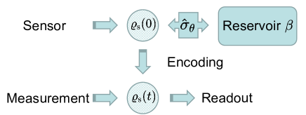
Figure 1: Schematic diagram of our quantum thermometry scheme in which a two-level system is used to as the sensor estimate the temperature of a bosonic reservoir.

In this section, we propose our scheme and analyze its sensing efficiency. A two-level system or a qubit, acting as the quantum sensor, is employed to estimate the temperature of a bosonic reservoir (see Fig. 1). The total Hamiltonian of the sensor plus the finite-temperature reservoir is described as follows:

$$\hat{H}=\hat{H}_{\mathrm{s}}+\sum_{k}\omega_{k}\hat{b}_{k}^{\dagger}\hat{b}_{k}+\mathcal{\hat{S}}\otimes\sum_{k}g_{k}(\hat{b}_{k}^{\dagger}+\hat{b}_{k}),$$ (3)

where $\hat{H}_{\mathrm{s}}=\frac{1}{2}\epsilon\hat{\sigma}_{z}+\frac{1}{2}\Delta\hat{\sigma}_{x}$ is the Hamiltonian of the sensor with $\epsilon$ being the bias and $\Delta$ being the tunneling parameter, operators $\hat{b}_{k}$ and $\hat{b}_{k}^{\dagger}$ are annihilation and creation operators of the $k$th bosonic mode with frequency $\omega_{k}$, respectively. The parameter $g_{k}$ labels the coupling strength between the sensor and the $k$th bosonic mode. Generally, it is very convenient to encode the frequency dependence of the interaction strengths in the so-called spectral density, which is defined by $J(\omega)\equiv\sum_{k}g_{k}^{2}\delta(\omega-\omega_{k})$. In this paper, we consider an Ohmic spectral density with a Drude-type cutoff

$$J(\omega)=\frac{2}{\pi}\frac{\chi\omega\omega_{\mathrm{c}}}{\omega^{2}+\omega_{\mathrm{c}}^{2}},$$ (4)

where $\chi$ qualifies the sensor-reservoir coupling strength, and $\omega_{\mathrm{c}}$ denotes the cutoff frequency.

In our scheme, we consider a general coupling operator, i.e., $\mathcal{\hat{S}}$ has the form of Duan et al. (2020)

$$\mathcal{\hat{S}}=\hat{\sigma}_{\theta}\equiv\sin\theta\hat{\sigma}_{z}+\cos\theta\hat{\sigma}_{x}.$$ (5)

By varying the coupling angle $\theta$, all the directions on the $x$-$z$ plane of the Bloch sphere can be taken into account. In Refs. Sun et al. (2016); Lü et al. (2013); Acharyya et al. (2020); Ke and Zhao (2018), $\sin\theta\hat{\sigma}_{z}$ is named as the diagonal coupling term, while $\cos\theta\hat{\sigma}_{x}$ is called the off-diagonal coupling operator. However, such a naming convention may lead to misunderstanding when the diagonal and the off-diagonal terms are included in both $\hat{H}_{\mathrm{s}}$ and $\mathcal{\hat{S}}$ at the same time. To avoid such a problem, in this paper, we prefer to use the $z$-type and $x$-type coupling terms to indicate $\sin\theta\hat{\sigma}_{z}$ and $\cos\theta\hat{\sigma}_{x}$ in $\mathcal{\hat{S}}$, respectively. Due to the rotational symmetry of $\hat{\sigma}_{\theta}$, we restrict our study to $0\leq\theta<\pi$. If $\theta=\pi/2$, a more $z$-type coupling operator is included in $\mathcal{\hat{S}}$; when $\theta=0$, only the $x$-type coupling is considered Sun et al. (2016). As demonstrated in Refs. Sun et al. (2016); Wu et al. (2012); Lü et al. (2013), the authors demonstrated the $x$-type coupling term plays a positive role in restraining coherence and can lead to a much richer ground-state phase diagram in the spin-boson systems. These results inspire us to explore the effect of $z$-type and $x$-type coupling on sensitivity of quantum thermometry.

To realize our sensing scheme, we assume the whole sensor-reservoir system is initially prepared in a product state

$$\begin{split}\varrho_{\mathrm{sb}}(0)=&\varrho_{\mathrm{s}}(0)\otimes\varrho_{\mathrm{b}}^{\mathrm{G}}\\ =&|\psi_{\mathrm{s}}(0)\rangle\langle\psi_{\mathrm{s}}(0)|\otimes\frac{\exp(-\beta\hat{H}_{\mathrm{b}})}{\mathrm{Tr}_{\mathrm{b}}[\exp(-\beta\hat{H}_{\mathrm{b}})]},\end{split}$$ (6)

where $|\psi_{\mathrm{s}}(0)\rangle=\cos\alpha|\mathrm{e}\rangle+\sin\alpha e^{-i\varphi}|g\rangle$ with $|\mathrm{e},g\rangle$ being the eigenstates of the Pauli $z$-operator and $\hat{H}_{\mathrm{b}}=\sum_{k}\omega_{k}\hat{b}_{k}^{\dagger}\hat{b}_{k}$ denotes the Hamiltonian of the reservoir. The parameter $\beta\equiv T^{-1}$ denotes the inverse temperature and is the quantity of interest to be estimated in this paper.

During the purely numerical calculations to the QFI, one needs to handle the first-order derivative to the parameter $\beta$, say $\partial_{\beta}\boldsymbol{r}$ in Eq. (2). In this paper, the first-order derivative for an arbitrary $\beta$-dependent function $f_{\beta}$ is numerically done by adopting the following finite difference method:

$$\partial_{\beta}f_{\beta}\simeq\frac{-f_{\beta+2\delta}+8f_{\beta+\delta}-8f_{\beta-\delta}+f_{\beta-2\delta}}{12\delta}.$$ (7)

We set $\delta/\beta=10^{-6}$, which provides a very good accuracy.

III.1 Non-Markovian temperature sensing

In this subsection, we first investigate the dynamical behavior of QFI within an exact non-Markovian framework. Depending on the characteristic of the reservoir spectral density, quantum reservoirs can be roughly classified into two different categories: the fast reservoir $\omega_{\mathrm{c}}>\max\{\epsilon,\Delta\}$ and the slow reservoir $\omega_{\mathrm{c}}\leq\max\{\epsilon,\Delta\}$ Ke and Zhao (2018); Lee et al. (2012); Wang et al. (2019). An interesting question arises here: what is the influence of the reservoir’s characteristic on the sensing performance? In this subsection, we try to address this question.

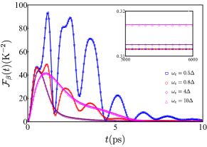
Figure 2: The dynamics QFI with different cutoff frequencies: $\omega_{\mathrm{c}}=0.5\Delta$ (blue rectangles), $\omega_{\mathrm{c}}=0.8\Delta$ (red circles), $\omega_{\mathrm{c}}=4\Delta$ (purple rhombuses) and $\omega_{\mathrm{c}}=10\Delta$ (magenta triangles). The inset figure depicts the steady-state QFI in the long-time regime. Parameters are chosen as $\alpha=\pi/4$, $\varphi=\pi/2$, $\epsilon=0.5\Delta$, $\beta\Delta=0.06$, $\theta=0$ and $\chi=0.06\Delta$ with $\Delta=1\,\mathrm{cm}^{-1}$.

We first consider the so-called deep fast-reservoir regime, i.e., $\omega_{\mathrm{c}}\gg\max\{\epsilon,\Delta\}$, in which the reservoir is memoryless (see Fig. 6 in Appendix A and Refs. Ke and Zhao (2018); Lee et al. (2012); Wang et al. (2019); Clos and Breuer (2012) for more details). In this regime, the dynamical behavior of QFI from the HEOM approach is displayed by the magenta triangles in Fig. 2. One can see the QFI gradually increases from its initial value $\mathcal{F}_{\beta}(0)=0$ to the maximum value. Then, the QFI begins to decrease and eventually tends to a steady value in the long-encoding-time limit. Such behavior of $\mathcal{F}_{\beta}(t)$ is physically reasonable because the whole temperature-sensing process includes the following three steps. First, no message about the temperature is contained in the initial state of the sensor, resulting in $\mathcal{F}_{\beta}(0)=0$ at the beginning. Then, the sensor-reservoir interaction, which generates the temperature’s information in $\varrho_{\mathrm{s}}(t)$ with the evolution of encoding time, leads to the increase of QFI. Finally, in the long-time limit, the value of $\mathcal{F}_{\beta}(t)$ remains unchanged because, in this step, the message about the temperature is completely from the steady-state reduced density matrix $\varrho_{\mathrm{s}}(\infty)$, which is independent of the encoding time. The above result means there exists an optimal encoding time which can maximize the value of QFI. The appearance of maximal QFI can be understood as the physical result of the interplay between the encoding and the decoherence  Wu and Shi (2020); Wu et al. (2021a, b); Bina et al. (2018). In Fig. 3, we plot the maximal QFI, $\max_{t}\mathcal{F}_{\beta}$, as a function of the coupling angle $\theta$. One can see the maximal QFI is quite sensitive to the coupling angle. Using our above results, one can design the most efficient sensor-reservoir interaction Hamiltonian to obtain the maximum precision estimation by adjusting the weight of the $x$-type coupling operator in the whole sensor-reservoir interaction Hamiltonian.

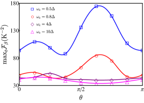
Figure 3: The maximum QFI with respect to the optimal encoding time versus the coupling angle for different cutoff frequencies: $\omega_{\mathrm{c}}=0.5\Delta$ (blue rectangles), $\omega_{\mathrm{c}}=0.8\Delta$ (red circles), $\omega_{\mathrm{c}}=4\Delta$ (purple rhombuses) and $\omega_{\mathrm{c}}=10\Delta$ (magenta triangles). Other parameters are the same as those of Fig. 2.

Next, we consider the slow-reservoir regime, for example, the blue rectangles with $\omega_{\mathrm{c}}=0.5\Delta$ in Fig. 2, in which the reservoir-induced decoherence should be strongly non-Markovian Ke and Zhao (2018); Lee et al. (2012); Wang et al. (2019). In this situation, we find the dynamics of QFI presented by the HEOM method exhibits a collapse-and-revival phenomenon resulting in multiple local maximums, which is completely different from that of the fast reservoir case. A similar result was also reported in Refs. Berrada (2013); Wu and Shi (2020) and can be regarded as evidence of the information’s backflow from the reservoir back to the sensor. Moreover, we also display the maximum QFI with respect to the optimal encoding time versus the coupling angle in Fig. 3. Multiple local-most-efficient coupling angles are revealed (see the the blue rectangles in Fig. 3). Additionally, we find the maximal QFI in the slow-reservoir regime can be much larger than that of the fast-reservoir case for the entire range of $0\leq\theta<\pi$. This result suggests the non-Markovian effect, generated by the characteristics of slow reservoir, may be used to improve the estimation precision.

III.2 Breakdown of the canonical statistics

In this subsection, we shall discuss the feature of steady-state QFI in the long-encoding-time regime. If the sensor-reservoir coupling is weak, the long-time steady state of a fully thermalized thermometer can be described by the canonical Gibbs state, namely, $\varrho_{\mathrm{s}}(\infty)\simeq\varrho_{\mathrm{s}}^{\mathrm{G}}=\exp(-\beta\hat{H}_{\mathrm{s}})/\mathrm{Tr}[\exp(-\beta\hat{H}_{\mathrm{s}})]$. In such an approximate treatment, by diagonalizing $\hat{H}_{\mathrm{s}}$, one can easily find the ratio of $\varrho_{\mathrm{gg}}(\infty)/\varrho_{\mathrm{ee}}(\infty)$ is a monotonously and exponentially increasing function

$$\frac{\varrho_{\mathrm{gg}}(\infty)}{\varrho_{\mathrm{ee}}(\infty)}\simeq\frac{\varrho_{\mathrm{gg}}^{\mathrm{G}}}{\varrho_{\mathrm{ee}}^{\mathrm{G}}}=e^{\beta\Omega},$$ (8)

where $\Omega=\sqrt{\epsilon^{2}+\Delta^{2}}$ shall be regarded as the sensor’s Rabi frequency. And the corresponding QFI with respect to the canonical Gibbs state is given by

$$\mathcal{F}_{\beta}^{\mathrm{G}}=\frac{\Omega^{2}}{2+2\cosh(\beta\Omega)}.$$ (9)

From the above expression, one can easily find $\mathcal{F}_{\beta}^{\mathrm{G}}(\Omega)$ is not a monotonic function. With a fixed temperature, $\mathcal{F}_{\beta}^{\mathrm{G}}(\Omega)$ is a increasing function for $\Omega\in[0,\Omega^{*})$ with $\Omega^{*}$ being determined by $\partial_{\Omega}\mathcal{F}_{\beta}^{\mathrm{G}}(\Omega)=0$; while, for $\Omega\in[\Omega^{*},\infty)$, $\mathcal{F}_{\beta}^{\mathrm{G}}(\Omega)$ monotonically decreases. The above analysis means the steady-state behaviors of the population ratio and the QFI strongly depend on the sensor’s Rabi frequency $\Omega$.

However, as demonstrated in many previous articles Lee et al. (2012); Gan and Zheng (2009); Zhao et al. (2011); Li et al. (2011), in the deep slow-reservoir regime, which generally induces a strongly non-Markovian effect, the reservoir-induced decoherence can give rise to a drastic frequency renormalization, namely, $\Omega\rightarrow\tilde{\Omega}$. The renormalized frequency $\tilde{\Omega}$ is smaller than the original frequency $\Omega$ and their deviation becomes larger as the increase of the sensor-reservoir coupling Lee et al. (2012); Gan and Zheng (2009); Zhao et al. (2011); Li et al. (2011); Silbey and Harris (1984). This result can be qualitatively understood by performing a polaron transformation. Making use of the polaron transformation, as displayed in Appendix B, the sensor’s Rabi frequency is renormalized as

$$\tilde{\Omega}_{\mathrm{P}}=\sqrt{\tilde{\epsilon}^{2}+\eta^{2}\tilde{\Delta}^{2}},$$ (10)

where $\tilde{\epsilon}=\epsilon\sin\theta+\Delta\cos\theta$, $\tilde{\Delta}=\Delta\sin\theta-\epsilon\cos\theta$, and $\eta$ is the renormalized factor, whose explicit expression is given by Eq. (B8), induced by the polaron transformation. In Table 1, we display the frequency renormalization within the framework of polaron transformation theory $\tilde{\Omega}_{\mathrm{P}}/\Omega$ versus the sensor-reservoir coupling strength $\chi$. It is clear to see a larger $\chi$ leads to a smaller $\tilde{\Omega}_{\mathrm{P}}/\Omega$. Such a frequency renormalization phenomenon is responsible for the so-called localized-delocalized transition in the well-known spin-boson model Gan and Zheng (2009); Zhao et al. (2011).

Table 1: The frequency renormalization $\tilde{\Omega}_{\mathrm{P}}$ and $\tilde{\Omega}_{\mathrm{H}}$ versus the sensor-reservoir coupling strength $\chi$. Parameters are chosen as $\alpha=\pi/4$, $\varphi=\pi/2$, $\theta=2\pi/3$, $\epsilon=2\Delta$, $\beta\Delta=0.95$, $\omega_{\mathrm{c}}=0.8\Delta$, and $\Delta=0.1\mathrm{cm}^{-1}$.

$\chi/\Delta$	0	0.1	0.2	0.3	0.4	0.5
$\tilde{\Omega}_{\mathrm{P}}/\Omega$	1.000	0.968	0.932	0.890	0.837	0.741
$\tilde{\Omega}_{\mathrm{H}}/\Omega$	1.000	0.834	0.818	0.794	0.766	0.734

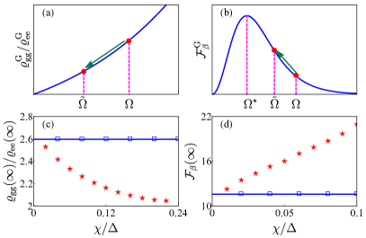
Figure 4: Schematic diagram of the influence of frequency renormalization $\Omega\rightarrow\tilde{\Omega}$ on (a) the steady-state population ratio and (b) the QFI. (c) The steady-state population ratio $\varrho_{\mathrm{gg}}(\infty)/\varrho_{\mathrm{ee}}(\infty)$ is plotted as a function of the sensor-reservoir coupling strength $\chi$. (d) The steady-state QFI versus $\chi$. The red five-point stars are the numerical results obtained by the HEOM method, the blue rectangles are the steady-state solutions from the Born-Markov master equation approach, while the blue solid lines represent the results from the canonical Gibbs state. Parameters are chosen as $\alpha=\pi/4$, $\varphi=\pi/2$, $\epsilon=0.5\Delta$, $\beta\Delta=5$, and $\omega_{\mathrm{c}}=0.5\Delta$ with $\Delta=50\,\mathrm{cm}^{-1}$. Here, $\Omega^{*}\simeq 24\,\mathrm{cm}^{-1}$ and $\Omega\simeq 56\,\mathrm{cm}^{-1}$.

Thus, the most simple and straightforward correction to the previous assumption of canonical statistics is replacing the original Rabi frequency $\Omega$ by a smaller renormalized frequency $\tilde{\Omega}$. Under such treatment, one can see the frequency shift $\Omega\rightarrow\tilde{\Omega}$ shall lead to a smaller value of $\varrho_{\mathrm{gg}}(\infty)/\varrho_{\mathrm{ee}}(\infty)$ [see Figs. 4(a) and 5(a)] compared with that of the canonical Gibbs state case, which implies the breakdown of canonical statistics Zhu et al. (2020); Iles-Smith et al. (2014, 2016). Moreover, if $\Omega>\Omega^{*}$, the frequency renormalization results in a larger QFI in comparison with that of the canonical statistics [see Fig. 4(b)]. On the contrary, if $\Omega<\Omega^{*}$, the frequency renormalization in turn diminishes the sensing precision [see Fig. 5(b)].

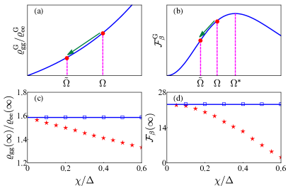
Figure 5: The same with Fig. 4, but $\beta\Delta=1$ and $\Delta=10\,\mathrm{cm}^{-1}$. Here, $\Omega^{*}\simeq 24\,\mathrm{cm}^{-1}$ and $\Omega\simeq 11\,\mathrm{cm}^{-1}$.

The above analytical analysis is completely based on the polaron transformation, which only provides a qualitative interpretation as well as a pictorial illustration. To obtain a quantitative result, we display the steady-state population ratio and the QFI as functions of the coupling strength from the HEOM and the Born-Markov master equation methods (see Appendix A for details) in Figs. 4(c,) and 4(d) and Figs. 5(c,) and 5(d). As a result of neglecting the higher-order terms of the sensor-reservior interaction, the steady-state solutions from the Born-Markov master equation approach coincide with the canonical statistics, i.e., the steady-state population ratio and the QFI are independent of the coupling strength. In sharp contrast to this, one can see the numerical results obtained by the HEOM method are in good agreement with our previous discussions about the frequency renormalization within the framework of the polaron transformation. In Table 1, we also display the renormalized Rabi frequency predicted by the HEOM method, namely $\tilde{\Omega}_{\mathrm{H}}\equiv\beta^{-1}\ln[\varrho_{\mathrm{gg}}(\infty)/\varrho_{\mathrm{ee}}(\infty)]$, as the function of the coupling strength $\chi$. It is clear to see the evolutionary trend of $\tilde{\Omega}_{\mathrm{H}}/\Omega$ in qualitative agreement with that of $\tilde{\Omega}_{\mathrm{P}}/\Omega$. These results demonstrate, in the strong-coupling regime, the noncanonical distribution occurs, which plays a complicated role in the quantum thermometry. The result presented by the red stars in Figs. 4(c,) and 4(d) and Figs. 5(c,)and 5(d) cannot be predicted by using the Gorini-Kossakowski-Sudarshan-Lindblad master equation formula or other common perturbative methods, where the effect of frequency shift is generally washed out Huang and Zheng (2010); Wu and Lin (2016).

Therefore, we uncover a threshold $\Omega=\Omega^{*}$, above such critical Rabi frequency, i.e., $\Omega>\Omega^{*}$, the sensing precision can be effectively enhanced by strengthening the sensor-reservoir coupling. In this sense, the sensitivity of quantum thermometry can be improved by engineering the sensor’s bare frequency. Here, we concentrate the frequency renormalization mechanism on the slow-reservoir regime, the reason is twofold. First, in the deep fast-reservoir regime, the decoherence is Markovian which means the canonical statistics assumption is valid with no need for corrections. Second, as $\omega_{\mathrm{c}}/\max\{\epsilon,\Delta\}\rightarrow\infty$, the renormalized factor $\eta$ approaches to $1$ accordingly, resulting in the disappearance of frequency shift phenomenon in the deep-reservoir regime. Our result is consistent with that of Ref. Correa et al. (2017), in which the authors found the sensing precision of a Brownian thermometer can be improved by increasing the coupling at low temperature. Their result can be easily understood by using our threshold mechanism: the critical Rabi frequency $\Omega^{*}$ approaches to zero in the low-temperature limit, which means the condition $\Omega>\Omega^{*}$ becomes very easy to be satisfied. Thus, as long as the Brownian sensor has a finite bare frequency, i.e., $\Omega>0$, the sensor-reservoir can boost the thermometric precision without doubt. Of course, it is worth mentioning that our scenario is totally different from that found in Ref. Correa et al. (2017). Their quantum thermometry is based on the Caldeira-Leggett Hamiltonian, namely, the sensor in Ref. Correa et al. (2017) is a continuous-variable system, rather than the discrete-variable sensor (qubit) in this paper.

IV Conclusion

In summary, going beyond the usual assumptions of the Born-Markov theory, the pure dephasing mechanism and the weak-coupling approximation, we propose a single-qubit thermometer scheme and analyze its sensing performance with the help of the HEOM approach. We find, when the encoding time is short and the sensor is partly thermalized, the non-Markovian effect induced by the slow reservoir’s characteristics may enhance the efficiency of the quantum thermometry. By optimizing the encoding time, we investigate the relation between the maximal QFI and the sensor-reservoir coupling angle. It is revealed that the performance of our quantum thermometry can be further boosted by modulating the weight of the $x$-type coupling operator in the whole sensor-reservoir Hamiltonian. Moreover, in the slow-reservoir regime, by strengthening the sensor-reservoir coupling, we find the noncanonical feature appears in the sensor’s steady state and the corresponding QFI obtained by the HEOM method can be larger than the value predicated by the canonical Gibbs state as well as the Born-Markov master equation approach, under suitable conditions. A possible threshold mechanism, which is based on the frequency renormalization appearing in the strongly non-Markovian regime, is proposed to explain the above result in the long-encoding-time limit. Finally, due to the generality of the qubit-based quantum thermometer, we expect our results to be of interest for certain potential applications in the researches of quantum metrology and quantum sensing.

V Acknowledgments

The authors thank Dr. Si-Yuan Bai, Professor Jun-Hong An and Professor Hong-Gang Luo for many fruitful discussions. W. Wu wishes to especially thank Dr. Chong Chen and an anonymous referee for their suggestions on the discussion of frequency renormalization. The work was supported by the National Natural Science Foundation (Grant No. 11704025).

VI Appendix A: HEOM

The HEOM method is a purely numerical technique, which exactly maps the Schr$\ddot{\mathrm{o}}$dinger equation or quantum Liouville equation to a set of ordinary differential equations by introducing auxiliary density matrices. These ordinary differential equations can be treated numerically by the Runge-Kutta algorithm. Without invoking the Born-Markov, weak-coupling and rotating-wave approximations, the HEOM can provide a rigorous numerical dynamics for an open quantum system Tanimura and Kubo (1989); Tanimura (1990, 2020); Xu and Yan (2007); Jin et al. (2007, 2008); Wu (2018a, b).

To realize the above HEOM method, it is generally required that the reservoir correlation function $C(t)$, which is defined by

$$\begin{split}C(t)=&\mathrm{Tr}_{\mathrm{b}}\Big{(}e^{it\hat{H}_{\mathrm{b}}}\mathcal{\hat{B}}e^{-it\hat{H}_{\mathrm{b}}}\mathcal{\hat{B}}\Big{)}\\ =&\int_{0}^{\infty}d\omega J(\omega)\Big{[}\coth\Big{(}\frac{\beta\omega}{2}\Big{)}\cos(\omega t)-i\sin(\omega t)\Big{]},\end{split}$$ (A1)

can be expressed as a sum of exponential functions Tanimura and Kubo (1989); Tanimura (1990, 2020); Xu and Yan (2007); Jin et al. (2007, 2008); Wu (2018a, b); Ritschel and Eisfeld (2014). Here, $\mathcal{\hat{B}}\equiv\sum_{k}g_{k}(\hat{b}_{k}^{\dagger}+\hat{b}_{k})$. Fortunately, for the Ohmic spectral density considered in this paper, the reservoir correlation function satisfies such requirement. Substituting Eq. (4) into Eq. (A1), one can find

$$C(t)=\sum_{\ell=0}^{\varepsilon}\zeta_{\ell}e^{-\upsilon_{\ell}t},$$ (A2)

where $\upsilon_{\ell}=\omega_{\mathrm{c}}\delta_{0\ell}+2\ell\pi(1-\delta_{0\ell})\beta^{-1}$ denotes the $\ell$th Matsubara frequency and

$$\begin{split}\zeta_{\ell}=&\frac{4\chi\omega_{\mathrm{c}}}{\beta}\frac{\upsilon_{\ell}}{\upsilon_{\ell}^{2}-\omega_{\mathrm{c}}^{2}}(1-\delta_{0\ell})\\ &+\Big{[}\chi\omega_{\mathrm{c}}\cot\Big{(}\frac{\beta\omega_{\mathrm{c}}}{2}\Big{)}-i\chi\omega_{\mathrm{c}}\Big{]}\delta_{0\ell},\end{split}$$ (A3)

are the expansion coefficients. Here, we set a truncation parameter $\varepsilon$ to ensure the above series remain finite. With the help of the Eq. (A2), the hierarchical equations can be constructed following detailed exposition in Refs. Wu (2018a, b). The HEOM reads

$$\begin{split}\frac{d}{dt}\varrho_{\vec{\nu}}(t)=&\Big{(}\mathcal{\hat{L}}_{\mathrm{s}}-\vec{\nu}\cdot\vec{\mu}\Big{)}\varrho_{\vec{\nu}}(t)\\ &+\hat{\Phi}\sum_{\ell=0}^{\varepsilon}\hat{\varrho}_{\vec{\nu}+\vec{e}_{\ell}}(t)+\sum_{\ell=0}^{\varepsilon}\nu_{\ell}\hat{\Theta}_{\ell}\hat{\varrho}_{\vec{\nu}-\vec{e}_{\ell}}(t),\end{split}$$ (A4)

where $\vec{\nu}=(\nu_{0},\nu_{1},\nu_{2},.~{}.~{}.,\nu_{\varepsilon})$ is a $(\varepsilon+1)$-dimensional index, $\vec{e}_{\ell}=(0,0,0,.~{}.~{}.1_{\ell},.~{}.~{}.,0)$ and $\vec{\mu}=(\upsilon_{0},\upsilon_{1},\upsilon_{2},.~{}.~{}.,\upsilon_{\varepsilon})$ are $(\varepsilon+1)$-dimensional vectors. The superoperators $\mathcal{\hat{L}}_{\mathrm{s}}$, $\hat{\Phi}$, and $\hat{\Theta}_{\ell}$ are defined as $\mathcal{\hat{L}}_{\mathrm{s}}\equiv-i\hat{H}_{\mathrm{s}}^{\times}$, $\hat{\Phi}\equiv-i\mathcal{\hat{S}}^{\times}$ and

$$\hat{\Theta}_{\ell}=-i\Big{[}\mathrm{Re}(\zeta_{\ell})\mathcal{\hat{S}}^{\times}+i\mathrm{Im}(\zeta_{\ell})\mathcal{\hat{S}}^{\circ}\Big{]},$$ (A5)

where $\hat{o}_{1}^{\times}\hat{o}_{2}\equiv\hat{o}_{1}\hat{o}_{2}-\hat{o}_{2}\hat{o}_{1}$ and $\hat{o}_{1}^{\circ}\hat{o}_{2}\equiv\hat{o}_{1}\hat{o}_{2}+\hat{o}_{2}\hat{o}_{1}$.

In numerical simulations, the initial states of the auxiliary operators are given by

$$\varrho_{\vec{\nu}=\vec{0}}(0)=\varrho_{\mathrm{s}}(0);~{}~{}\varrho_{\vec{\nu}\neq\vec{0}}(0)=\vec{0},$$ (A6)

where $\vec{0}=(0,0,0...,0)$ is a $(\varepsilon+1)$-dimensional zero vector. In this paper, we constantly increasing the number of the differential equations as well as the value of $\varepsilon$ until the final result converges.

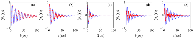
Figure 6: The dynamics of population difference $\langle\hat{\sigma}_{z}(t)\rangle$ with different cutoff frequencies: (a) $\omega_{\mathrm{c}}=30\Delta$ (the deep fast-reservoir regime), (b) $\omega_{\mathrm{c}}=20\Delta$, (c) $\omega_{\mathrm{c}}=10\Delta$, (d) $\omega_{\mathrm{c}}=0.07\Delta$, and (e) $\omega_{\mathrm{c}}=0.05\Delta$ (the deep slow-reservoir regime). The red circles are numerical results predicted by the HEOM method, while the blue solid lines are from the Born-Markovian master equation approach. Other parameters are chosen as $\alpha=\pi/4$, $\varphi=\pi/2$, $\epsilon=0.5\Delta$, $\chi=0.06\Delta$, $\beta\Delta=0.25$, $\theta=3\pi/8$, and $\Delta=1\,\mathrm{cm}^{-1}$.

As a benchmark, we also employe the most common Born-Markov master equation to compute the reduced dynamics of the sensor. As displayed in Ref. Wu and Lin (2016), the Born-Markov master equation reads

$$\frac{d}{dt}\varrho_{\mathrm{s}}(t)=\Big{(}\mathcal{\hat{L}}_{\mathrm{s}}-\mathcal{\hat{S}}^{\times}\hat{\Upsilon}^{\times}+\mathcal{\hat{S}}^{\times}\hat{\Xi}^{\circ}\Big{)}\varrho_{\mathrm{s}}(t),$$ (A7)

where

$$\hat{\Upsilon}\equiv\int_{0}^{\infty}dtC_{\mathrm{R}}(t)\mathcal{\hat{S}}(-t),$$

and

$$\hat{\Xi}\equiv-i\int_{0}^{\infty}dtC_{\mathrm{I}}(t)\mathcal{\hat{S}}(-t).$$

Here, $\mathcal{\hat{S}}(t)\equiv e^{it\hat{H}_{\mathrm{s}}}\hat{\mathcal{S}}e^{-it\hat{H}_{\mathrm{s}}}$ and $C_{\mathrm{R}(\mathrm{I})}(t)$ denotes the real (imaginary) part of the correlation function. By neglecting the imaginary Lamb-shift terms Wu and Lin (2016), the master equation given by Eq. (A7) can be further simplified, which shall be very convenient for numerical simulations in practice.

To verify the feasibility of the HEOM method, we here make a comparison between the purely numerical result obtained by the numerical HEOM method and that of the Born-Markov master equation approach. In Fig. 6, we display the evolution of population difference

$$\langle\hat{\sigma}_{z}(t)\rangle\equiv\mathrm{Tr}\Big{[}\hat{\sigma}_{z}e^{-i\hat{H}t}\varrho_{\mathrm{s}}(0)\otimes\varrho_{\mathrm{b}}^{\mathrm{G}}e^{i\hat{H}t}\Big{]}.$$ (A8)

Good agreement is found between results from the two different approaches in the deep fast-reservoir regime, see Fig. 6(a). On the contrary, a relatively large deviation is found in the deep slow-reservoir regime, see Figs. 66(d) and 6(e). Moreover, we observe that such a deviation becomes more and more evident as $\omega_{\mathrm{c}}/\Delta$ approaches to zero with fixed $\epsilon=0.5\Delta$. This result is physically reasonable, because the reservoir is memoryless in the deep fast-reservoir regime. While, with the decrease of $\omega_{\mathrm{c}}/\Delta$, the non-Markovianity becomes non-negligible Clos and Breuer (2012), which means the results from the Born-Marovian master equation method are unreliable. Our result is consistent with that of Ref. Ke and Zhao (2018) in which only the $z$-type coupling term is taken into consideration.

VII Appendix B: Variational polaron transformation

To obtain the explicit expression of $\tilde{\Omega}_{\mathrm{P}}$, we first need a rotation matrix $\mathcal{\hat{R}}\equiv\exp(-\frac{i}{2}\phi\hat{\sigma}_{y})$ with $\phi=\arctan(\cot\theta)$ to diagonalize $\mathcal{\hat{S}}$. By doing so, the original Hamiltonian $\hat{H}$ can be transformed into $\hat{H}^{\prime}=\mathcal{\hat{R}}^{\dagger}\hat{H}\mathcal{\hat{R}}$, where

$$\hat{H}^{\prime}=\frac{1}{2}\tilde{\epsilon}\hat{\sigma}_{z}+\frac{1}{2}\tilde{\Delta}\hat{\sigma}_{x}+\hat{H}_{\mathrm{b}}+\hat{\sigma}_{z}\otimes\sum_{k}\tilde{g}_{k}(\hat{b}_{k}^{\dagger}+\hat{b}_{k}),$$ (B1)

with $\tilde{g}_{k}=\sin(\theta+\phi)g_{k}$. For the special scope $0\leq\theta<\pi$ considered in this paper, $\tilde{g}_{k}$ coincidentally reduces to $g_{k}$. Employing such rotation, $\hat{H}^{\prime}$ now has the standard form of well-known spin-boson model.

Next, we apply the variational polaron transformation to $\hat{H}^{\prime}$ as $\hat{H}^{\prime\prime}=\exp(\hat{\mathcal{P}})\hat{H}^{\prime}\exp(-\hat{\mathcal{P}})$. Here, the polaron generator $\hat{\mathcal{P}}$ is given by Lee et al. (2012)

$$\hat{\mathcal{P}}=\hat{\sigma}_{z}\sum_{k}\frac{\xi_{k}}{\omega_{k}}(\hat{b}_{k}^{\dagger}-\hat{b}_{k}),$$ (B2)

where $\xi_{k}=g_{k}\mathfrak{S}(\omega_{k})$ with

$$\mathfrak{S}(\omega_{k})=\bigg{[}1+\frac{\eta^{2}\tilde{\Delta}^{2}}{\omega_{k}\tilde{\Omega}_{\mathrm{P}}}\coth\Big{(}\frac{1}{2}\beta\omega_{k}\Big{)}\tanh\Big{(}\frac{1}{2}\beta\tilde{\Omega}_{\mathrm{P}}\Big{)}\bigg{]}^{-1},$$ (B3)

being self-consistently determined by minimizing the Bogoliubov upper bound for the free energy Lee et al. (2012). The expression of $\hat{H}^{\prime\prime}$ can be written as $\hat{H}^{\prime\prime}=\hat{H}_{\mathrm{s}}^{\prime\prime}+\hat{H}_{\mathrm{b}}+\hat{H}_{\mathrm{sb}}^{\prime\prime}$, where $\hat{H}_{\mathrm{s}}^{\prime\prime}$ denotes the transformed Hamiltonian of the sensor

$$\hat{H}_{\mathrm{s}}^{\prime\prime}=\frac{1}{2}\tilde{\epsilon}\hat{\sigma}_{z}+\frac{1}{2}\eta\tilde{\Delta}\hat{\sigma}_{x}+\sum_{k}\frac{\xi_{k}}{\omega_{k}}\big{(}\xi_{k}-2g_{k}\big{)}.$$ (B4)

The last term in the above expression is an energy shift induced by the polaron transformation, which has no influence on the sensing accuracy in the assumption of canonical statistics. From the expression of $\hat{H}_{\mathrm{s}}^{\prime\prime}$, one can immediately find the Rabi frequency is $\tilde{\Omega}_{\mathrm{P}}^{2}=\tilde{\epsilon}^{2}+\eta^{2}\tilde{\Delta}^{2}$, which recovers Eq. (10) in the main text. The transformed sensor-reservoir interaction Hamiltonian $\hat{H}_{\mathrm{sb}}^{\prime\prime}$ can be written as $\hat{H}_{\mathrm{sb}}^{\prime\prime}=\hat{\sigma}_{x}\mathcal{\hat{B}}_{x}+\hat{\sigma}_{y}\mathcal{\hat{B}}_{y}+\hat{\sigma}_{z}\mathcal{\hat{B}}_{z}$, where

$$\mathcal{\hat{B}}_{x}=\frac{1}{2}\tilde{\Delta}\big{(}\cosh\hat{\Sigma}-\eta\big{)},~{}~{}\mathcal{\hat{B}}_{y}=\frac{i}{2}\tilde{\Delta}\sinh\hat{\Sigma},$$ (B5)

$$\begin{split}\mathcal{\hat{B}}_{z}=\sum_{k}\big{(}g_{k}-\xi_{k}\big{)}\Big{(}\hat{b}_{k}^{\dagger}+\hat{b}_{k}\Big{)},\end{split}$$ (B6)

with

$$\hat{\Sigma}\equiv\sum_{k}\frac{2\xi_{k}}{\omega_{k}}\Big{(}\hat{b}_{k}^{\dagger}-\hat{b}_{k}\Big{)},$$ (B7)

and

$$\begin{split}\eta\equiv&\mathrm{Tr}\Big{(}\varrho_{\mathrm{b}}^{\mathrm{G}}\cosh\hat{\Sigma}\Big{)}\\ =&\exp\bigg{[}-2\int_{0}^{\infty}d\omega\frac{J(\omega)}{\omega^{2}}\mathfrak{S}(\omega)^{2}\coth\Big{(}\frac{1}{2}\beta\omega\Big{)}\bigg{]}.\end{split}$$ (B8)

References

- Puglisi et al. (2017) A. Puglisi, A. Sarracino, and A. Vulpiani, “Temperature in and out of equilibrium: A review of concepts, tools and attempts,” Physics Reports 709-710, 1–60 (2017).
- Mehboudi et al. (2019) Mohammad Mehboudi, Anna Sanpera, and Luis A Correa, “Thermometry in the quantum regime: recent theoretical progress,” Journal of Physics A: Mathematical and Theoretical 52, 303001 (2019).
- Mitchison et al. (2020) Mark T. Mitchison, Thomás Fogarty, Giacomo Guarnieri, Steve Campbell, Thomas Busch, and John Goold, “In situ thermometry of a cold fermi gas via dephasing impurities,” Phys. Rev. Lett. 125, 080402 (2020).
- Hovhannisyan et al. (2021) Karen V. Hovhannisyan, Mathias R. Jørgensen, Gabriel T. Landi, Álvaro M. Alhambra, Jonatan B. Brask, and Martí Perarnau-Llobet, “Optimal quantum thermometry with coarse-grained measurements,” PRX Quantum 2, 020322 (2021).
- Mok et al. (2021) Wai-Keong Mok, Kishor Bharti, Leong-Chuan Kwek, and Abolfazl Bayat, “Optimal probes for global quantum thermometry,” Communications Physics 4, 62 (2021).
- Kirkova et al. (2021) Aleksandrina V. Kirkova, Weibin Li, and Peter A. Ivanov, “Adiabatic sensing technique for optimal temperature estimation using trapped ions,” Phys. Rev. Research 3, 013244 (2021).
- Cavina et al. (2018) Vasco Cavina, Luca Mancino, Antonella De Pasquale, Ilaria Gianani, Marco Sbroscia, Robert I. Booth, Emanuele Roccia, Roberto Raimondi, Vittorio Giovannetti, and Marco Barbieri, “Bridging thermodynamics and metrology in nonequilibrium quantum thermometry,” Phys. Rev. A 98, 050101(R) (2018).
- Feyles et al. (2019) Michele M. Feyles, Luca Mancino, Marco Sbroscia, Ilaria Gianani, and Marco Barbieri, “Dynamical role of quantum signatures in quantum thermometry,” Phys. Rev. A 99, 062114 (2019).
- Tamascelli et al. (2020) Dario Tamascelli, Claudia Benedetti, Heinz-Peter Breuer, and Matteo G A Paris, “Quantum probing beyond pure dephasing,” New Journal of Physics 22, 083027 (2020).
- Correa et al. (2017) Luis A. Correa, Martí Perarnau-Llobet, Karen V. Hovhannisyan, Senaida Hernández-Santana, Mohammad Mehboudi, and Anna Sanpera, “Enhancement of low-temperature thermometry by strong coupling,” Phys. Rev. A 96, 062103 (2017).
- Hovhannisyan and Correa (2018) Karen V. Hovhannisyan and Luis A. Correa, “Measuring the temperature of cold many-body quantum systems,” Phys. Rev. B 98, 045101 (2018).
- Khan et al. (2021) M. Miskeen Khan, H. Terças, J. T. Mendonça, J. Wehr, C. Charalambous, M. Lewenstein, and M. A. Garcia-March, “Quantum dynamics of a bose polaron in a -dimensional bose-einstein condensate,” Phys. Rev. A 103, 023303 (2021).
- Correa et al. (2015) Luis A. Correa, Mohammad Mehboudi, Gerardo Adesso, and Anna Sanpera, “Individual quantum probes for optimal thermometry,” Phys. Rev. Lett. 114, 220405 (2015).
- Potts et al. (2019) Patrick P. Potts, Jonatan Bohr Brask, and Nicolas Brunner, “Fundamental limits on low-temperature quantum thermometry with finite resolution,” Quantum 3, 161 (2019).
- Pati et al. (2020) Arun Kumar Pati, Chiranjib Mukhopadhyay, Sagnik Chakraborty, and Sibasish Ghosh, “Quantum precision thermometry with weak measurements,” Phys. Rev. A 102, 012204 (2020).
- Latune et al. (2020) C L Latune, I Sinayskiy, and F Petruccione, “Collective heat capacity for quantum thermometry and quantum engine enhancements,” New Journal of Physics 22, 083049 (2020).
- Gebbia et al. (2020) Francesca Gebbia, Claudia Benedetti, Fabio Benatti, Roberto Floreanini, Matteo Bina, and Matteo G. A. Paris, “Two-qubit quantum probes for the temperature of an ohmic environment,” Phys. Rev. A 101, 032112 (2020).
- Bouton et al. (2020) Quentin Bouton, Jens Nettersheim, Daniel Adam, Felix Schmidt, Daniel Mayer, Tobias Lausch, Eberhard Tiemann, and Artur Widera, “Single-atom quantum probes for ultracold gases boosted by nonequilibrium spin dynamics,” Phys. Rev. X 10, 011018 (2020).
- Candeloro and Paris (2021) Alessandro Candeloro and Matteo G. A. Paris, “Discrimination of ohmic thermal baths by quantum dephasing probes,” Phys. Rev. A 103, 012217 (2021).
- Kenfack et al. (2021) Lionel Tenemeza Kenfack, William Degaulle Waladi Gueagni, Martin Tchoffo, and Lukong Cornelius Fai, “Temperature estimation in a quantum spin bath through entangled and separable two-qubit probes,” The European Physical Journal Plus 136, 220 (2021).
- Vázquez and Gorin (2020) P C López Vázquez and T Gorin, “Probing the dynamics of an open quantum system via a single qubit,” Journal of Physics A: Mathematical and Theoretical 53, 355301 (2020).
- Campbell et al. (2018) Steve Campbell, Marco G Genoni, and Sebastian Deffner, “Precision thermometry and the quantum speed limit,” Quantum Science and Technology 3, 025002 (2018).
- Liu et al. (2019) Jing Liu, Haidong Yuan, Xiao-Ming Lu, and Xiaoguang Wang, “Quantum fisher information matrix and multiparameter estimation,” Journal of Physics A: Mathematical and Theoretical 53, 023001 (2019).
- Xiong et al. (2015) Heng-Na Xiong, Ping-Yuan Lo, Wei-Min Zhang, Da Hsuan Feng, and Franco Nori, “Non-markovian complexity in the quantum-to-classical transition,” Scientific Reports 5, 13353 (2015).
- Cai et al. (2014) C. Y. Cai, Li-Ping Yang, and C. P. Sun, “Threshold for nonthermal stabilization of open quantum systems,” Phys. Rev. A 89, 012128 (2014).
- Yang et al. (2014) Chun-Jie Yang, Jun-Hong An, Hong-Gang Luo, Yading Li, and C. H. Oh, “Canonical versus noncanonical equilibration dynamics of open quantum systems,” Phys. Rev. E 90, 022122 (2014).
- Matsuzaki et al. (2018) Yuichiro Matsuzaki, Simon Benjamin, Shojun Nakayama, Shiro Saito, and William J. Munro, “Quantum metrology beyond the classical limit under the effect of dephasing,” Phys. Rev. Lett. 120, 140501 (2018).
- Berrada (2013) K. Berrada, “Non-markovian effect on the precision of parameter estimation,” Phys. Rev. A 88, 035806 (2013).
- Wu and Shi (2020) Wei Wu and Chuan Shi, “Quantum parameter estimation in a dissipative environment,” Phys. Rev. A 102, 032607 (2020).
- Wu et al. (2021a) Wei Wu, Si-Yuan Bai, and Jun-Hong An, “Non-markovian sensing of a quantum reservoir,” Phys. Rev. A 103, L010601 (2021a).
- Wu et al. (2021b) Wei Wu, Zhen Peng, Si-Yuan Bai, and Jun-Hong An, “Threshold for a discrete-variable sensor of quantum reservoirs,” Phys. Rev. Applied 15, 054042 (2021b).
- Salari Sehdaran et al. (2019) Fahimeh Salari Sehdaran, Mohammad H. Zandi, and Alireza Bahrampour, “The effect of probe-ohmic environment coupling type and probe information flow on quantum probing of the cutoff frequency,” Physics Letters A 383, 126006 (2019).
- Tanimura and Kubo (1989) Yoshitaka Tanimura and Ryogo Kubo, “Time evolution of a quantum system in contact with a nearly gaussian-markoffian noise bath,” Journal of the Physical Society of Japan 58, 101–114 (1989).
- Tanimura (1990) Yoshitaka Tanimura, “Nonperturbative expansion method for a quantum system coupled to a harmonic-oscillator bath,” Phys. Rev. A 41, 6676–6687 (1990).
- Tanimura (2020) Yoshitaka Tanimura, “Numerically “exact” approach to open quantum dynamics: The hierarchical equations of motion (heom),” The Journal of Chemical Physics 153, 020901 (2020).
- Xu and Yan (2007) Rui-Xue Xu and YiJing Yan, “Dynamics of quantum dissipation systems interacting with bosonic canonical bath: Hierarchical equations of motion approach,” Phys. Rev. E 75, 031107 (2007).
- Jin et al. (2007) Jinshuang Jin, Sven Welack, JunYan Luo, Xin-Qi Li, Ping Cui, Rui-Xue Xu, and YiJing Yan, “Dynamics of quantum dissipation systems interacting with fermion and boson grand canonical bath ensembles: Hierarchical equations of motion approach,” The Journal of Chemical Physics 126, 134113 (2007).
- Jin et al. (2008) Jinshuang Jin, Xiao Zheng, and YiJing Yan, “Exact dynamics of dissipative electronic systems and quantum transport: Hierarchical equations of motion approach,” The Journal of Chemical Physics 128, 234703 (2008).
- Wu (2018a) Wei Wu, “Realization of hierarchical equations of motion from stochastic perspectives,” Phys. Rev. A 98, 012110 (2018a).
- Wu (2018b) Wei Wu, “Stochastic decoupling approach to the spin-boson dynamics: Perturbative and nonperturbative treatments,” Phys. Rev. A 98, 032116 (2018b).
- Hauke et al. (2016) Philipp Hauke, Markus Heyl, Luca Tagliacozzo, and Peter Zoller, “Measuring multipartite entanglement through dynamic susceptibilities,” Nature Physics 12, 778–782 (2016).
- Lambert and Sørensen (2019) J. Lambert and E. S. Sørensen, “Estimates of the quantum fisher information in the antiferromagnetic heisenberg spin chain with uniaxial anisotropy,” Phys. Rev. B 99, 045117 (2019).
- Haine and Hope (2020) Simon A. Haine and Joseph J. Hope, “Machine-designed sensor to make optimal use of entanglement-generating dynamics for quantum sensing,” Phys. Rev. Lett. 124, 060402 (2020).
- Huelga et al. (1997) S. F. Huelga, C. Macchiavello, T. Pellizzari, A. K. Ekert, M. B. Plenio, and J. I. Cirac, “Improvement of frequency standards with quantum entanglement,” Phys. Rev. Lett. 79, 3865–3868 (1997).
- Bai et al. (2019) Kai Bai, Zhen Peng, Hong-Gang Luo, and Jun-Hong An, “Retrieving ideal precision in noisy quantum optical metrology,” Phys. Rev. Lett. 123, 040402 (2019).
- Braunstein and Caves (1994) Samuel L. Braunstein and Carlton M. Caves, “Statistical distance and the geometry of quantum states,” Phys. Rev. Lett. 72, 3439–3443 (1994).
- Zhong et al. (2013) Wei Zhong, Zhe Sun, Jian Ma, Xiaoguang Wang, and Franco Nori, “Fisher information under decoherence in bloch representation,” Phys. Rev. A 87, 022337 (2013).
- Duan et al. (2020) Chenru Duan, Chang-Yu Hsieh, Junjie Liu, Jianlan Wu, and Jianshu Cao, “Unusual transport properties with noncommutative system–bath coupling operators,” The Journal of Physical Chemistry Letters 11, 4080–4085 (2020).
- Sun et al. (2016) Ke-Wei Sun, Yuta Fujihashi, Akihito Ishizaki, and Yang Zhao, “A variational master equation approach to quantum dynamics with off-diagonal coupling in a sub-ohmic environment,” The Journal of Chemical Physics 144, 204106 (2016).
- Lü et al. (2013) Zhiguo Lü, Liwei Duan, Xin Li, Prathamesh M. Shenai, and Yang Zhao, “Sub-ohmic spin-boson model with off-diagonal coupling: Ground state properties,” The Journal of Chemical Physics 139, 164103 (2013).
- Acharyya et al. (2020) Nirmalendu Acharyya, Roman Ovcharenko, and Benjamin P. Fingerhut, “On the role of non-diagonal system–environment interactions in bridge-mediated electron transfer,” The Journal of Chemical Physics 153, 185101 (2020).
- Ke and Zhao (2018) Yaling Ke and Yi Zhao, “Quantum dynamics simulations in an ultraslow bath using hierarchy of stochastic schrödinger equations,” Molecular Physics 116, 813–822 (2018).
- Wu et al. (2012) Ning Wu, Ke-Wei Sun, Zhe Chang, and Yang Zhao, “Resonant energy transfer assisted by off-diagonal coupling,” The Journal of Chemical Physics 136, 124513 (2012).
- Lee et al. (2012) Chee Kong Lee, Jeremy Moix, and Jianshu Cao, “Accuracy of second order perturbation theory in the polaron and variational polaron frames,” The Journal of Chemical Physics 136, 204120 (2012).
- Wang et al. (2019) Yu-Chen Wang, Yaling Ke, and Yi Zhao, “The hierarchical and perturbative forms of stochastic schrödinger equations and their applications to carrier dynamics in organic materials,” WIREs Computational Molecular Science 9, e1375 (2019).
- Clos and Breuer (2012) Govinda Clos and Heinz-Peter Breuer, “Quantification of memory effects in the spin-boson model,” Phys. Rev. A 86, 012115 (2012).
- Bina et al. (2018) Matteo Bina, Federico Grasselli, and Matteo G. A. Paris, “Continuous-variable quantum probes for structured environments,” Phys. Rev. A 97, 012125 (2018).
- Gan and Zheng (2009) Congjun Gan and Hang Zheng, “Non-markovian dynamics of a dissipative two-level system: Nonzero bias and sub-ohmic bath,” Phys. Rev. E 80, 041106 (2009).
- Zhao et al. (2011) Chunjian Zhao, Zhiguo Lü, and Hang Zheng, “Entanglement evolution and quantum phase transition of biased spin-boson model,” Phys. Rev. E 84, 011114 (2011).
- Li et al. (2011) Haifeng Li, Jiushu Shao, and Shikuan Wang, “Derivation of exact master equation with stochastic description: Dissipative harmonic oscillator,” Phys. Rev. E 84, 051112 (2011).
- Silbey and Harris (1984) Robert Silbey and Robert A. Harris, “Variational calculation of the dynamics of a two level system interacting with a bath,” The Journal of Chemical Physics 80, 2615–2617 (1984).
- Zhu et al. (2020) Wen-Li Zhu, Wei Wu, and Hong-Gang Luo, “Effect of system–reservoir correlations on temperature estimation,” Chinese Physics B 29, 020501 (2020).
- Iles-Smith et al. (2014) Jake Iles-Smith, Neill Lambert, and Ahsan Nazir, “Environmental dynamics, correlations, and the emergence of noncanonical equilibrium states in open quantum systems,” Phys. Rev. A 90, 032114 (2014).
- Iles-Smith et al. (2016) Jake Iles-Smith, Arend G. Dijkstra, Neill Lambert, and Ahsan Nazir, “Energy transfer in structured and unstructured environments: Master equations beyond the born-markov approximations,” The Journal of Chemical Physics 144, 044110 (2016).
- Huang and Zheng (2010) Peihao Huang and Hang Zheng, “Effect of bath temperature on the quantum decoherence,” Chemical Physics Letters 500, 256–262 (2010).
- Wu and Lin (2016) Wei Wu and Hai-Qing Lin, “Effect of bath temperature on the decoherence of quantum dissipative systems,” Phys. Rev. A 94, 062116 (2016).
- Ritschel and Eisfeld (2014) Gerhard Ritschel and Alexander Eisfeld, “Analytic representations of bath correlation functions for ohmic and superohmic spectral densities using simple poles,” The Journal of Chemical Physics 141, 094101 (2014).