Adversarial Purification through Representation Disentanglement

Abstract

Deep learning models are vulnerable to adversarial examples and make incomprehensible mistakes, which puts a threat on their real-world deployment. Combined with the idea of adversarial training, preprocessing-based defenses are popular and convenient to use because of their task independence and good generalizability. Current defense methods, especially purification, tend to remove “noise” by learning and recovering the natural images. However, different from random noise, the adversarial patterns are much easier to be overfitted during model training due to their strong correlation to the images. In this work, we propose a novel adversarial purification scheme by presenting disentanglement of natural images and adversarial perturbations as a preprocessing defense. With extensive experiments, our defense is shown to be generalizable and make significant protection against unseen strong adversarial attacks. It reduces the success rates of state-of-the-art ensemble attacks from 61.7% to 14.9% on average, superior to a number of existing methods. Notably, our defense restores the perturbed images perfectly and does not hurt the clean accuracy of backbone models, which is highly desirable in practice.

Introduction

Adversarial examples have seriously threatened the application of deep learning models, which are mainly crafted by adding malicious perturbations to natural images (Szegedy et al. 2014; Goodfellow, Shlens, and Szegedy 2015; Madry et al. 2018; Dong et al. 2018, 2019). To enhance and harden the reliability of deep learning models, a large number of researchers are devoted to developing defenses to counter adversarial examples, such as adversarial training (Madry et al. 2018; Zhang et al. 2019) and input preprocessing defenses (Guo et al. 2018; Xie et al. 2018; Prakash et al. 2018; Liao et al. 2018; Naseer et al. 2020). Adversarial training methods are usually task-dependent, computationally expensive, and sacrifice models’ performances on clean data (Naseer et al. 2020). In contrast, input preprocessing defenses are scalable and task-agnostic.

Now we are discussing the design of preprocessing methods. While early input preprocessing methods (Guo et al. 2018; Xie et al. 2018; Prakash et al. 2018) are less robust to strong iterative attacks (Dong et al. 2019), the recently proposed purification defenses (Liao et al. 2018; Naseer et al. 2020) show more promising results by regarding the adversarial perturbation removal as a special case of denoising tasks. Popular deep denoising schemes (Zhang et al. 2017; Liu et al. 2018b) focus on learning the underlying image structures from the clean corpus. Thus, as the solver of the ill-posed inverse problem, i.e., denoising, the learned deep image prior can be applied to remove “noise” that is assumed random and uncorrelated to the clean images. In contrast, such assumption is no longer valid in adversarial purification, as the perturbations are generated based on the natural data, thus NOT random but highly correlated to the natural images. Most attack methods take the images as inputs and accumulate the gradients of models w.r.t inputs to craft adversarial examples. Thus, as existing purification defense algorithms all reply on fitting the mapping from adversarial samples to natural images, they inevitably overfit the adversarial patterns when constructing the deep image prior. We argue that such an overfitting issue by overlooking the fundamental differences between adversarial perturbations and random noise would limit the performances of existing purification-based defenses.

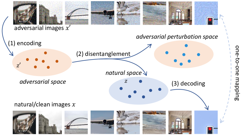
Figure 1: The pipeline of the proposed RDP for adversarial purification.

In this work, different from all existing methods, we tackle the adversarial perturbation challenge by learning to disentangle perturbation and natural images, based on which we propose a novel adversarial example purification method, called Representation Disentangled Purification (RDP). Concretely, RDP disentangles the latent vectors of natural images from adversarial latent space and recovers natural images in an end-to-end manner. Figure 1 shows the pipeline of the proposed RDP. RDP shows the best performances against various strong adversarial attacks through extensive experiments, compared to the state-of-the-art (SOTA) preprocessing-based defenses. Our contributions are summarized as follows:

• We propose a novel adversarial defense scheme named RDP, which effectively purifies the adversarial examples by disentangling natural image representations from adversarial perturbations.

• The RDP model is trained in a self-supervised manner with no assumption of potential adversarial attacks. Notably, RDP can be turned into a dynamic defense against strong white-box attacks.

• Extensive experimental results against various strong attacks on ImageNet demonstrate the efficacy and superiority of RDP.

Related Works

Adversarial Attacks

Since Szegedy et al. (2014) for the first time revealed the vulnerability of deep learning models on adversarial examples, numerous attack methods are proposed to generate imperceptible adversarial perturbations. Goodfellow, Shlens, and Szegedy (2015) proposed an one-step attack: Fast Gradient Sign Method (FGSM) to generate adversarial examples quickly; Later, the multi-step FGSM (I-FGSM) is developed in (Kurakin, Goodfellow, and Bengio 2016) to generate strong attacks. Some similar attacks are C&W attack (Carlini and Wagner 2017), JSMA (Papernot et al. 2016), and PGD attack (Madry et al. 2018). To enhance the transferability and practicality of strong attacks, Momentum is introduced in the process of generation, called MI-FGSM (Dong et al. 2018). More recently, Xie et al. (2019b) proposed to augment the input with randomized scaling and padding to boost the transferability, the attack of which is called DI-FGSM; Dong et al. (2019) and Lin et al. (2020) utilized the translation-invariant and scale-invariant properties of convolutional neural networks (CNNs), and developed corresponding TI-FGSM and SI-FGSM attacks respectively. All these attacks are generated as a function of the input images.

Adversarial Defenses

One widely recognized defense method is called adversarial training (Madry et al. 2018; Zhang et al. 2019), which involves adversarial examples during training, and many variants of adversarial training have been proposed (Bai et al. 2021). Though effective, there are many challenges of adversarial training remaining to solve, like high training cost, task dependency, and the trade-off between accuracy and adversarial robustness for adversarial trained models (Naseer et al. 2020; Bai et al. 2021), which hinder the broad application of adversarially trained models. Compared to adversarial training, another line of research relies on image restoration techniques to remove adversarial perturbations before feeding images to downstream tasks. Guo et al. (2018) used JPEG compression and Total Variation Minimization (TVM) to remove adversarial perturbations. Xu, Evans, and Qi (2017) proposed bit reduction (Bit-Red), which is designed to do feature squeezing to remove adversarial effects. Xie et al. (2018) preprocessed the input by Random resizing and Padding (R&P) to mitigate the effects of adversarial examples. Mustafa et al. (2019) employed super-resolution (SR) to map off-the-manifold adversarial samples back to the manifold of natural images. Jia et al. (2019) utilized deep models to compress input images and remove adversarial patterns, which is named as ComDefend. Liu et al. (2019) proposed Feature distillation (FD), which is a JPEG-based compression framework for defense purposes. Liao et al. (2018) adopted the denoiser with high-level representation guidance, which is named HGD. R&P and HGD are the top-2 solutions in NIPS 2017 Adversarial attacks and defenses competition (Kurakin et al. 2018). NRP (Naseer et al. 2020), the derivative work of HGD, employs a self-supervised way to generate adversarial examples for training denoisers. Energy-Based Models (EBM) trained with Markov-Chain Monte-Carlo (MCMC) (Yoon, Hwang, and Lee 2021; Grathwohl et al. 2020) show the efficacy for purifying adversarial examples from toy datasets. A large number of MCMC steps during training make these methods costly and impractical when applied to large datasets. The online purification method proposed by (Shi, Holtz, and Mishne 2021) requires an accompanied auxiliary task for training backbone models, which is task-dependant thus not considered in this paper.

Disentanglement for Adversarial Robustness

Disentanglement is designed to model the independent representations of data with variations, which has a wide range of applications in image translation (Liu et al. 2018a) and domain adaptation (Peng et al. 2019). In the field of adversarial defenses, some very recent works have demonstrated the efficacy of disentanglement in robust representation learning (Willetts et al. 2020; Yang et al. 2021; Gowal et al. 2020). To the best of our knowledge, no prior works apply disentanglement to adversarial purification. We are the first to exploit disentangling the natural representations from adversarial examples and restore their natural counterparts.

Methodology

In this section, we first elaborate on the architecture and the objective functions of RDP, then explain the motivation and advantages of the two-branch design of RDP.

RDP Framework

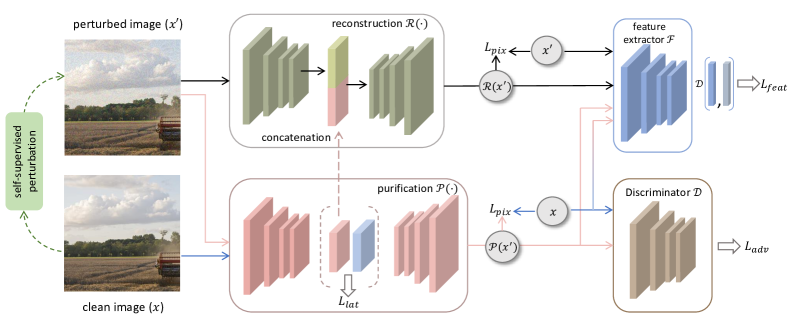
Figure 2: Illustration of proposed RDP network architecture.

The design of our RDP architecture is depicted in this section. As shown in Figure 2, RDP consists of a purifier $\mathcal{P}$, a reconstructor $\mathcal{R}$, a discriminator $\mathcal{D}$ and a feature extractor $\mathcal{F}$. The upper and lower branches in DRP are called the purification and reconstruction branches, respectively. The proposed RDP aims to learn a purifier $\mathcal{P}$ (purification branch) to purify adversarial patterns and restore natural images ($x$) from their adversarial examples ($x^{\prime}$), and utilize the reconstructor $\mathcal{R}$ (reconstruction branch) to reconstruct the perturbed images with the natural latent representations as the additional inputs. In this way, natural latent representations are disentangled from adversarial latent representations and used to recover purified images. The purified images are then discriminated by the discriminator $\mathcal{D}$ to ensure they are mapped onto the manifold of natural images. With the pre-trained feature extractor $\mathcal{F}$, we utilize the power of self-supervision for crafting adversarial examples, which makes our defense task-agnostic and is proved to be effective in (Naseer et al. 2020). During training, given natural images $x$, adversarial examples $x^{\prime}$ are crafted by maximizing the feature distortions of the feature extractor $\mathcal{F}$, which is expressed as

$$\begin{split}\max_{\boldsymbol{x}^{\prime}}\boldsymbol{d}\left(\mathcal{F}_{n}(\boldsymbol{x}),\mathcal{F}_{n}\left(\boldsymbol{x}^{\prime}\right)\right)\text{ s.t. }\left\|\boldsymbol{x}-\boldsymbol{x}^{\prime}\right\|_{\infty}\leq\epsilon,\end{split}$$ (1)

where $n$ is layer number of $\mathcal{F}$ used for feature extraction, $\epsilon$ is the maximum of perturbations under $l_{\infty}$ distance, and the function of $\boldsymbol{d}(\cdot)$ is to calculate the distance between two inputs. We use project gradient descent (Madry et al. 2018) to solve the Eq. (1) and obtain $x^{\prime}$. Then $x$ and $x^{\prime}$ are fed into RDP simultaneously. The training scheme is summarized in Algorithm 1.

Training Loss

For the purification branch, $x^{\prime}$ is expected to be mapped into the natural image manifold. The purified image $\mathcal{P}(x^{\prime})$ should be aligned to the natural image $x$ to a feasible extent. Thus, we designed a hybrid loss function for $\mathcal{P}$, which consists of latent representation loss, feature loss, pixel loss, and adversarial loss and is well explained in the following.

RDP is to disentangle the natural representations from adversarial examples and restore the natural counterparts. The restored images should be similar to the clean images as much as possible. We design the feature loss $\mathcal{L}_{feat}$ and pixel loss $\mathcal{L}_{pix}$ for restoring images from contents to styles, which are expressed as

$$\mathcal{L}_{feat}^{\mathcal{P}}=\left\|\mathcal{F}_{n}(\mathcal{P}(x^{\prime}))-\mathcal{F}_{n}(x)\right\|_{1}$$ (2)

and

$$\mathcal{L}_{pix}^{\mathcal{P}}=\left\|\mathcal{P}(x^{\prime})-x)\right\|_{1}.$$ (3)

We add latent representation loss $\mathcal{L}_{lat}$ for regularizing the latent representations extracted by the encoder, which is expressed as

$$\mathcal{L}_{lat}=\left\|\mathcal{P}_{enc}(x^{\prime})-\mathcal{P}_{enc}(x)\right\|_{1},$$ (4)

where $\mathcal{P}_{enc}(\cdot)$ represents the disentangled latent representations. Lastly, we use the adversarial loss $\mathcal{L}_{adv}$ to push the restored images to the manifold of natural images. We use the relativistic average GAN objective here for better convergence (Yadav, Chen, and Ross 2020; Jolicoeur-Martineau 2018; Naseer et al. 2020), which is

$$\mathcal{L}_{adv}=-\log\left(\sigma\left(\mathcal{D}_{\phi}\left(\mathcal{P}\left(\boldsymbol{x}^{\prime}\right)\right)-\mathcal{D}_{\phi}(\boldsymbol{x})\right)\right),$$ (5)

where $\sigma$ is the sigmoid function. The overall loss function of purification branch is

$$\mathcal{L}_{\mathcal{P}}=\mathcal{L}_{feat}^{\mathcal{P}}+\alpha_{1}\cdot\mathcal{L}_{pix}^{\mathcal{P}}+\alpha_{2}\cdot\mathcal{L}_{lat}+\alpha_{3}\cdot\mathcal{L}_{adv}.$$ (6)

On the other hand, the reconstruction branch is to reconstruct adversarial examples. It is worthy to note that the reconstructor $\mathcal{R}$ takes the latent representations extracted by $\mathcal{P}$ as input as well. Ideally, the natural latent representations from $\mathcal{P}$ are concatenated with the latent representations extracted by the encoder of $\mathcal{R}$, forming the integral adversarial latent representations for reconstruction. As such, the reconstruction and the purification branches complete the processing of disentanglement together. Thus, the reconstructed images $\mathcal{R}(x^{\prime})$ are expected to be similar to $x^{\prime}$ from the feature and pixel level, the losses of which are expressed as

$$\mathcal{L}_{feat}^{\mathcal{R}}=\left\|\mathcal{F}_{n}(\mathcal{R}(x^{\prime}))-\mathcal{F}_{n}(x^{\prime})\right\|_{1}$$ (7)

and

$$\mathcal{L}_{pix}^{\mathcal{R}}=\left\|\mathcal{R}(x^{\prime})-x^{\prime})\right\|_{1}.$$ (8)

Similarly, the overall loss for the reconstruction branch is

$$\mathcal{L}_{\mathcal{R}}=\mathcal{L}_{feat}^{\mathcal{R}}+\beta\cdot\mathcal{L}_{pix}^{\mathcal{R}}.$$ (9)

Algorithm 1 RDP training

Input: training data $\mathcal{X}$, Purifier $\mathcal{P}$, Reconstructor $\mathcal{R}$, feature extractor $\mathcal{F}$, discriminator $\mathcal{D}$, perturbation budget $\epsilon$, loss functions $\mathcal{L}_{\mathcal{P}}$ and $\mathcal{L}_{\mathcal{R}}$
Initialization: $\mathcal{P}$, $\mathcal{R}$ and $\mathcal{D}$

1:  while $\mathcal{P}$ doesn’t converge do

2:     Sample mini-batch of data $x\sim\mathcal{X}$.

3:     Obtain adversarial counterparts $x^{\prime}$ within the perturbation budget $\epsilon$ by solving Eq. (1).

4:     Feed $x$ and $x^{\prime}$ into $\mathcal{P}$, extract $V_{x^{\prime}}$ (the latent representations of $x^{\prime}$), and calculate $\mathcal{L}_{\mathcal{P}}$ (Eq. (6)).

5:     Feed $x^{\prime}$ and $V_{x^{\prime}}$ into $\mathcal{R}$ and calculate $\mathcal{L}_{\mathcal{R}}$ (Eq. (9)).

6:     Update $\mathcal{P}$ and $\mathcal{R}$ to minimize $\mathcal{L}_{\mathcal{P}}$ and $\mathcal{L}_{\mathcal{R}}$, respectively.

7:     Update $\mathcal{D}$ to classify $x$ from $\mathcal{P}(x^{\prime})$.

8:  end while

9:  return $\mathcal{P}$

Motivation of RDP Design

The design of RDP is to model both the natural images and their adversarial perturbations, which are different from random noise in two aspects. First, the distribution of adversarial perturbations is unknown. Random noise, due to Central Limit Theorem, is usually assumed to be under the Gaussian distribution (Meng and De la Torre 2013; Zhu et al. 2016). In contrast, as stated above, adversarial perturbations are dependant to images, which can be seen as a function of input images. The distribution of adversarial perturbations is difficult to model explicitly and remains unclear to us (Dong et al. 2020). Second, adversarial perturbations are correlated to image contents. From the perspective of the frequency domain, adversarial perturbations tend to have more high-frequency components that are mixed with the image contents while Gaussian noise does not (see Figure 3). As discovered in (Ulyanov, Vedaldi, and Lempitsky 2018), deep neural networks tend to learn the structural contents from corrupted images. The single-branch denoising methods inevitably would be overfitting to adversarial patterns during training, hurting the restoration of corrupted images.

By design, our two-branch RDP can handle these challenges. It is known that adversarial examples are crafted by adding adversarial perturbations to clean images. In our approach, as shown in Figure 2, we use the purification branch to restore clean images from adversarial inputs, and the reconstruction branch to reconstruct the adversarial inputs. On the one hand, the purification branch learns the distribution of natural images. On the other hand, the two branches are connected through latent representations. The adversarial images are recovered from the concatenated latent representations so that the distribution of adversarial perturbations is captured implicitly by RDP, which makes RDP superior to single-branch methods.

(a)

(b)

(c)

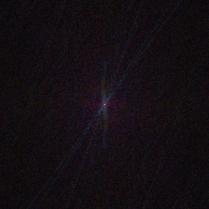
(d)

Figure 3: Differences between Gaussian noise and adversarial perturbations from the perspective of frequency domain. (a) and (c) are samples with Gaussian noise and adversarial perturbations, respectively. (b) and (d) plots the magnitudes of the noise and perturbation frequency spectrum in (a) and (c), respectively.

Experiments

Implementation details

Model Architecture

There are mainly four sub-models in RDP. The architectures of purifier $\mathcal{P}$ and the reconstructor $\mathcal{R}$ are adopted from (Wang et al. 2019; Kupyn et al. 2018), which consist of a convolutional layer and multiple basic blocks. Like Naseer et al. (2020) did, we remove the skip-connection to avoid introducing adversarial patterns to outputs. For the feature extractor $\mathcal{F}$ and the discriminator $\mathcal{D}$, their architectures are based on the VGG network, which is composed of five convolutional layers and one fully connected layer. Note that $\mathcal{F}$ is pre-trained on ImageNet (Russakovsky et al. 2015) and fixed during training.

Training Details

We implement our models and experiments with Python 3.8 and Pytorch 1.7 (Paszke et al. 2019) on three NVIDIA GTX 2080 Ti GPUs. For training, we randomly extract 25K images from the training data of ImageNet (Russakovsky et al. 2015) (25 images per class) as our training set. Adversarial examples are generated in a self-supervised way with $\epsilon=16$ and fed into RDP with their corresponding natural images. During training, we use randomly cropped images whose size is 128 × 128 × 3. The batch size is set to 48. Learning rates $\mathcal{R}$, $\mathcal{P}$ and $\mathcal{D}$ for are 0.0001. Hyperparameters are set to be $\alpha_{1,2,3}=\{10^{-2},10^{-1},10^{-4}\}$ and $\beta=10^{-4}$, respectively.

Evaluation Details

For evaluation, we mainly use NIPS 2017 DEV dataset (Kurakin et al. 2018), which contains $1,000$ images sampled from ImageNet. In our experiments, we study five models naturally pretrained on ImageNet: Inceptionv3 (Inc-v3) (Szegedy et al. 2016), Inceptionv4 (Inc-v4) (Szegedy et al. 2017), ResNet v2-101 (ResNet-101) (He et al. 2016) , ResNet v2-152 (ResNet-152) and Inception-ResNet-v2 (IncRes-v2) (Szegedy et al. 2017), and one adversarial trained model IncRes-v2_ens (Tramèr et al. 2018). Using the author-released codes, we evaluate our defense with various attacks like FGSM, MI-FGSM (iteration=10, momentum = 1)1, DIM (probability = 0.7), TI-DIM1, and SINI-TIDIM (scale = 5). Note that we only use the purification branch of RDP for evaluation.

Table 1: Error rates (%, lower is better) of different defense methods against various attacks ($\epsilon=16$). Other defenses are implemented based on author-released codes.

		Attacks
	Defense	FGSM	MI-FGSM	DIM	TI-DIM	SINI-TIDIM	Average
Inc-v3	JEPG	19.4	20.6	31.8	39.6	44.1	31.1
	FD	27.5	26.8	33.4	47.8	42.8	35.7
	Bit-Red	8.1	10.5	13.4	34.2	20.5	17.3
	TVM	10.0	13.8	18.6	37.8	27.7	21.6
	SR	28.0	28.9	44.3	40.8	43.7	37.1
	R&P	8.9	11.8	17.9	41.2	21.6	20.3
	ComDefend	22.5	22.5	27.3	44.3	37.3	30.8
	HGD	3.2	5.4	6.6	35.5	12.5	12.6
	NRP	5.5	6.8	9.1	12.7	13.2	9.5
	RDP	3.8	5.2	5.9	9.8	9.8	6.9
Inc-v4	JEPG	23.7	27.9	41.1	41.2	52.2	37.2
	FD	28.9	30.1	36.3	47.7	48.7	38.3
	Bit-Red	10.1	12.8	17.1	37.6	27.0	20.9
	TVM	11.8	17.7	22.4	39.4	35.7	25.4
	SR	33.7	40.2	54.5	47.1	52.1	45.5
	R&P	10.5	15.4	19.5	44.4	30.2	24.0
	ComDefend	24.6	25.3	30.3	45.7	44.8	34.1
	HGD	3.5	7.3	10.2	38.7	18.5	15.6
	NRP	6.9	7.6	9.3	13.0	18.0	11.0
	RDP	4.3	6.6	6.5	9.4	13.2	8.0
ResNet-101	JEPG	25.3	30.2	50.9	51.0	50.2	41.5
	FD	32.7	33.3	47.3	58.0	47.6	43.8
	Bit-Red	10.3	15.2	24.0	46.7	26.1	24.5
	TVM	14.1	21.4	34.8	48.2	35.1	30.7
	SR	35.8	38.0	57.8	46.4	49.0	45.4
	R&P	12.7	18.8	30.3	50.2	30.9	28.6
	ComDefend	25.7	25.8	36.2	55.3	41.8	37.0
	HGD	4.8	12.5	18.2	47.5	20.1	20.6
	NRP	9.3	11.6	15.7	22.2	18.9	15.5
	RDP	6.0	8.9	10.7	20.6	15.3	12.3
ResNet-152	JEPG	25.5	28.2	48.9	52.1	48.1	40.6
	FD	31.1	30.1	45.1	57.5	46.6	42.1
	Bit-Red	10.5	14.9	25.3	48.8	25.9	25.1
	TVM	13.1	19.2	34.2	48.3	33.0	29.6
	SR	34.1	35.7	57.4	45.0	47.5	43.9
	R&P	10.9	18.0	30.2	51.2	28.1	27.7
	ComDefend	25.1	24.0	36.7	56.2	38.7	36.1
	HGD	4.7	10.3	18.9	48.7	18.7	20.3
	NRP	8.3	10.0	16.1	21.5	17.0	14.6
	RDP	5.9	7.7	11.7	19.9	13.3	11.7
ensemble	JEPG	31.0	57.3	74.1	69.5	61.9	58.8
	FD	34.9	50.3	64.6	68.6	52.6	54.2
	Bit-Red	12.6	26.4	38.5	65.0	26.9	33.9
	TVM	16.2	35.8	51.2	66.6	35.3	41.0
	SR	38.8	61.0	82.1	65.2	61.3	61.7
	R&P	13.1	32.1	48.4	70.2	29.3	38.6
	ComDefend	30.5	42.7	57.1	68.8	45.1	48.8
	HGD	4.0	17.1	25.5	68.2	16.0	26.2
	NRP	11.1	18.5	25.9	31.5	18.1	21.0
	RDP	5.5	13.1	16.7	26.2	13.0	14.9

Table 2: Clean accuracy (higher is better) of different defenses. We use red$\uparrow$ to indicate the results which are higher than the original accuracy of IncRes-v2_ens on clean images.

Defense	JEPG	FD	BIT	TVM	SR
Acc	97.40%	90.30%	97.20%	96.20%	97.70% red$\uparrow$
Defense	R&P	ComDefend	HGD	NRP	RDP
Acc	97.10%	90.50%	97.20%	94.90%	97.70% red$\uparrow$

Table 3: Success rates (higher is better) of RDP against BPDA and TI-DIM attacks.

	ResNet-152	ResNet-152	ResNet-152 NRP
	TI-DIM	TI-DIM	TI-DIM BPDA
With RDP	✗	✓	✓
Inc-v3	37.10%	71.50%	64.60%
Inc-v4	43.10%	75.40%	71.90%
Incres-v2	45.60%	83.60%	83.10%
IncRes-v2ens	50.20%	80.80%	79.20%

Table 4: Defense success rates (higher is better) against PGD-10 attack in white-box settings on ImageNet validation set (50k images). ResNet-152 is used as the backbone.

Defense	N/A	AT-FD	NRP	RDP
Clean	82.41%	65.30%	73.86%	81.40%
Adversarial	0.74%	55.70%	65.60%	71.30%

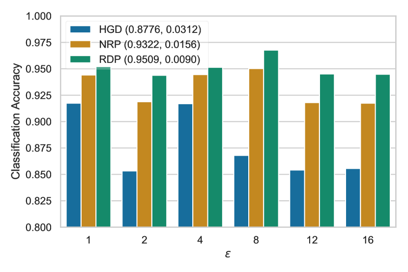
Figure 4: Success rates of HGD, NRP and RDP when defending against various attacks with $\epsilon=1,2,4,8,12,16$. The mean and standard deviation of each method are behind their names. We use Inc-v3 as the source model for attacks and IncRes-v2 as the backbone.

Evaluation Results

FGSM: bullfrog (✗)

MI-FGSM: bullfrog (✗)

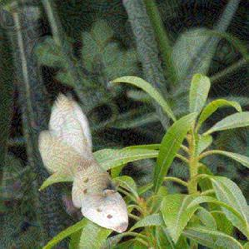
DIM: bullfrog (✗)

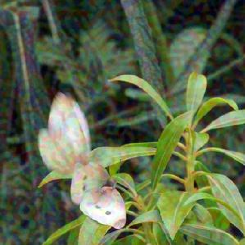
TI-DIM: corn (✗)

SINI-TIDIM: kingsnake (✗)

Sulphur butterfly (✓)

Sulphur butterfly (✓)

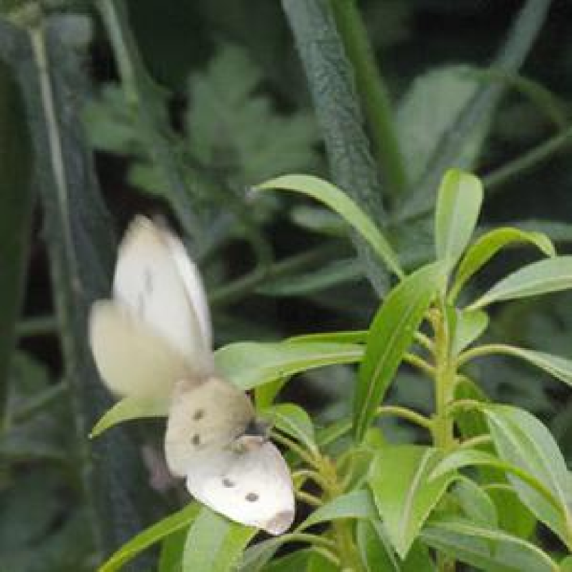
Sulphur butterfly (✓)

Sulphur butterfly (✓)

Sulphur butterfly (✓)

Figure 5: An illustration of the generalizability of RDP against various strong attacks ($\epsilon=16$). Images on the top row are generated by different adversarial attacks, while images on the bottom row are purified by RDP. RDP effectively removes the adversarial patterns and maintains the samples in high quality. we use ✓and ✗ to indicate the correctness of predictions, where IncRes-v2_ens is used as the backbone.

Defending various attacks

Compared to adversarial training, one advantage of preprocessing-based defenses is that there is no assumption of the potential attacks and downstream tasks. To demonstrate the generalization ability, RDP is deployed to defend against various strong attacks like FGSM, MI-FGSM, DIM, TI-DIM and SINI-TIDIM, where $\epsilon\in[0,255]$ and is set as 16 under $l_{\infty}$ norm, four naturally trained models and their ensembles are used as the source models. We also compare RDP with previous representative methods like JPEG compression (Guo et al. 2018), TVM (Guo et al. 2018), Bit Depth Reduction (Bit-Red) (Xu, Evans, and Qi 2017), Feature Distillation (FD) (Liu et al. 2019), SR (Mustafa et al. 2019), R&P (Xie et al. 2018), ComDefend (Jia et al. 2019) and the state-of-the-art methods like HGD (Liao et al. 2018) and NRP (Naseer et al. 2020). All these methods are originally developed to defend adversarial examples with $\epsilon=16$ on ImageNet. IncRes-v2_ens is used as the backbone model here. Quantitative results are summarized in Table 1. As we can see, among those methods, RDP holds the strongest robustness when defending most attacks. HGD performs better than RDP when defending FGSM, the reason of which is that the training data of HGD contains a large portion of adversarial examples generated by FGSM (Liao et al. 2018) while we don’t assume the potential attacks when training RDP. Compared to the SOTA method NRP, RDP holds an improvement of $3.6\%$ on average. In addition, RDP doesn’t hurt the performances of the backbone model on clean data while other defenses sacrifice the accuracy (97.60%) of the backbone model up to 7.10% (see Table 2).

Defending attacks with varying $\epsilon$

The magnitude $\epsilon$ of attacks is usually fixed for both training and testing in the literature (Liao et al. 2018; Naseer et al. 2020). Nevertheless, we argue that this could conceal the overfitting issue of learning-based defenses. The potential risk of being overfitting would make defenses unreliable to weak attacks. To address this concern, we prepare another evaluation set consisting of adversarial examples generated by the same attacks but with varying $\epsilon=\{1,2,4,8,12,16\}$, which is missing in the literature. Inc-v3 is used here as the target model for attacks. We mainly choose HGD and NRP for comparison, which are the most relevant to RDP and have good performances in previous experiments. As illustrated in Figure 4, across various $\epsilon$, the mean value of classification accuracies defended by RDP is highest, and the standard deviation is the smallest. To conclude, RDP generalizes well across various attacks with different $\epsilon$, the performances of which are more stable than NRP and HGD.

Adversaries’ Awareness of Defenses

In the above experiments, we assume the adversaries have no idea about the defenses. However, as suggested in (Athalye, Carlini, and Wagner 2018), adversaries could approximate the gradients to evade defenses when defenses are deployed. Here, we investigate the performances of RDP in this difficult scenario. We make two primary assumptions of the adversaries: (1) the adversaries are aware of the existence of our defense and have access to the exact or similar training data, (2) the adversaries train a similar defense and combines it with BPDA (Athalye, Carlini, and Wagner 2018) and TI-DIM attack to bypass our defense. Here we use the current SOTA method: NRP (Naseer et al. 2020) as the adversaries’ local defense and ResNet-152 as the source model to simulate this attack. Three naturally-trained models and one adversarially-trained model are used for evaluation. The experimental results are summarized in Table 3. For attacks with BPDA, the performances of RDP only drop slightly. What’s more, with RDP as the defense, the average relative gain of four target models is 74%. To sum up, RDP can effectively defend against adversarial attacks and is resistant to BPDA.

Further, we consider the worst scenario where adversaries can access both RDP and the backbone model when launching attacks. Following (Xie et al. 2019a), we test RDP under the targeted PGD-10 attack with $\epsilon=16$ in white-box settings. For hardening our defense, we propose to make RDP dynamic by incorporating random smoothing strategy (Cohen, Rosenfeld, and Kolter 2019; Naseer et al. 2020). Specifically, we add one Gaussian noise layer (standard deviation is 0.05) on the top of RDP when inference. In Table 4, we demonstrate the efficacy of RDP defending against white-box attacks. RDP significantly improves the robustness of the backbone model while maintaining the clean accuracy, which is apparently superior to adversarial training with feature denoising (AT-FD) (Xie et al. 2019a).

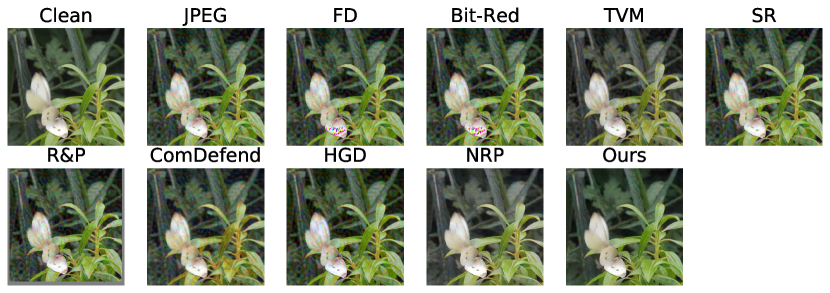
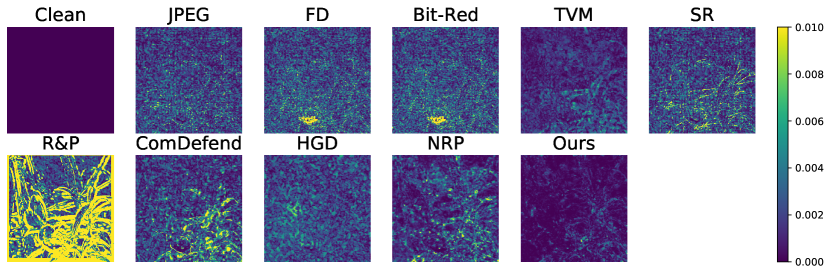
Figure 6: Restoration results (upper) and the magnitudes of the corresponding errors (lower) by different defense methods. The darker, the better. Adversarial example purified by RDP preserves the highest similarity with the clean image.

Disentangled Outputs by RDP

As illustrated in Figure 2, RDP has two branches: purification and reconstruction. When defending against adversarial attacks, we only use the purification branch. Samples of different adversarial examples and their corresponding purified images by RDP are shown in Figure 5. We also show the processed adversarial examples by other defenses in Figure 6. By visualizing the error maps between the processed images and clean images, we could see that RDP has the best restoration ability, which is also reflected in the strong adversarial robustness of RDP.

For better understanding the usage of the reconstruction branch in RDP, given an adversarial example (Figure 7(a)), we visualize and show the disentangled outputs of two branches in Figure 7(b) and 7(c), respectively. Further, we fix the reconstruction branch’s latent vector and replace the purification branch’s latent vector with random noise. The new reconstruction output is shown in Figure 7(d), which indicates that RDP does disentangle the contents and the perturbations of adversarial examples.

(a)

(b)

(c)

(d)

Figure 7: Disentangled outputs of RDP. (a) is the adversarial example. (b) and (c) are the outputs of purification and reconstruction branches, respectively. (d) is the output of reconstruction branch when replacing the natural latent vector with random noise.

Ablation Study

Here, we thoroughly investigate the impact of disentanglement training and the use of different objective functions with our defense. Figure 8 shows the evaluation results and provides the following conclusions: (1) the reconstruction branch indeed helps the purification of adversarial examples; (2) Performances of RDP without latent loss, pixel loss, and adversarial loss drop slightly; (3) Without feature loss, RDP cannot project adversarial examples to the manifold of natural images, and the defense gets much weaker.

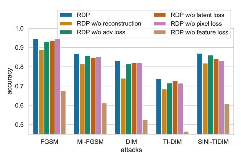
Figure 8: Ablation study of RDP. Results are obtained by IncRes-v2_ens against the ensemble attacks in previous experiments.

Conclusion

This paper proposes a novel defense method called Representation Disentangled Purification (RDP) to defend against adversarial attacks. By disentangling the image content and adversarial patterns, RDP effectively recovers the clean images in high quality. With extensive experiments, RDP exhibits high generalizability to the unseen strong attacks and outperforms the existing SOTA defense methods by a large gap. The high generalizability makes RDP potentially be applied to many kinds of downstream attacks and provides high adversarial robustness. Incorporating with the dynamic strategy, RDP is also resistant to strong white-box attacks without sacrificing the clean accuracy of backbone models.

References

- Athalye, Carlini, and Wagner (2018) Athalye, A.; Carlini, N.; and Wagner, D. 2018. Obfuscated gradients give a false sense of security: Circumventing defenses to adversarial examples. In International conference on machine learning, 274–283. PMLR.
- Bai et al. (2021) Bai, T.; Luo, J.; Zhao, J.; Wen, B.; and Wang, Q. 2021. Recent Advances in Adversarial Training for Adversarial Robustness. arXiv preprint arXiv:2102.01356.
- Carlini and Wagner (2017) Carlini, N.; and Wagner, D. 2017. Towards evaluating the robustness of neural networks. In 2017 IEEE Symposium on Security and Privacy (SP). IEEE.
- Cohen, Rosenfeld, and Kolter (2019) Cohen, J. M.; Rosenfeld, E.; and Kolter, J. Z. 2019. Certified Adversarial Robustness via Randomized Smoothing. In Proceedings of the 36th International Conference on Machine Learning, ICML 2019, 9-15 June 2019, Long Beach, California, USA, Proceedings of Machine Learning Research.
- Dong et al. (2020) Dong, Y.; Deng, Z.; Pang, T.; Zhu, J.; and Su, H. 2020. Adversarial Distributional Training for Robust Deep Learning. In Advances in Neural Information Processing Systems 33: Annual Conference on Neural Information Processing Systems 2020, NeurIPS 2020, December 6-12, 2020, virtual.
- Dong et al. (2018) Dong, Y.; Liao, F.; Pang, T.; Su, H.; Zhu, J.; Hu, X.; and Li, J. 2018. Boosting Adversarial Attacks With Momentum. In 2018 IEEE Conference on Computer Vision and Pattern Recognition, CVPR 2018, Salt Lake City, UT, USA, June 18-22, 2018.
- Dong et al. (2019) Dong, Y.; Pang, T.; Su, H.; and Zhu, J. 2019. Evading Defenses to Transferable Adversarial Examples by Translation-Invariant Attacks. In IEEE Conference on Computer Vision and Pattern Recognition, CVPR 2019, Long Beach, CA, USA, June 16-20, 2019.
- Goodfellow, Shlens, and Szegedy (2015) Goodfellow, I. J.; Shlens, J.; and Szegedy, C. 2015. Explaining and Harnessing Adversarial Examples. In 3rd International Conference on Learning Representations, ICLR 2015, San Diego, CA, USA, May 7-9, 2015, Conference Track Proceedings.
- Gowal et al. (2020) Gowal, S.; Qin, C.; Huang, P.-S.; Cemgil, T.; Dvijotham, K.; Mann, T.; and Kohli, P. 2020. Achieving robustness in the wild via adversarial mixing with disentangled representations. In Proceedings of the IEEE/CVF Conference on Computer Vision and Pattern Recognition, 1211–1220.
- Grathwohl et al. (2020) Grathwohl, W.; Wang, K.-C.; Jacobsen, J.-H.; Duvenaud, D.; Norouzi, M.; and Swersky, K. 2020. Your classifier is secretly an energy based model and you should treat it like one. In International Conference on Learning Representations.
- Guo et al. (2018) Guo, C.; Rana, M.; Cissé, M.; and van der Maaten, L. 2018. Countering Adversarial Images using Input Transformations. In 6th International Conference on Learning Representations, ICLR 2018, Vancouver, BC, Canada, April 30 - May 3, 2018, Conference Track Proceedings.
- He et al. (2016) He, K.; Zhang, X.; Ren, S.; and Sun, J. 2016. Identity mappings in deep residual networks. In European conference on computer vision, 630–645. Springer.
- Jia et al. (2019) Jia, X.; Wei, X.; Cao, X.; and Foroosh, H. 2019. Comdefend: An efficient image compression model to defend adversarial examples. In Proceedings of the IEEE/CVF Conference on Computer Vision and Pattern Recognition, 6084–6092.
- Jolicoeur-Martineau (2018) Jolicoeur-Martineau, A. 2018. The relativistic discriminator: a key element missing from standard GAN. arXiv preprint arXiv:1807.00734.
- Kupyn et al. (2018) Kupyn, O.; Budzan, V.; Mykhailych, M.; Mishkin, D.; and Matas, J. 2018. Deblurgan: Blind motion deblurring using conditional adversarial networks. In Proceedings of the IEEE conference on computer vision and pattern recognition, 8183–8192.
- Kurakin et al. (2018) Kurakin, A.; Goodfellow, I.; Bengio, S.; Dong, Y.; Liao, F.; Liang, M.; Pang, T.; Zhu, J.; Hu, X.; Xie, C.; et al. 2018. Adversarial attacks and defences competition. In The NIPS’17 Competition: Building Intelligent Systems, 195–231. Springer.
- Kurakin, Goodfellow, and Bengio (2016) Kurakin, A.; Goodfellow, I. J.; and Bengio, S. 2016. Adversarial examples in the physical world. CoRR.
- Liao et al. (2018) Liao, F.; Liang, M.; Dong, Y.; Pang, T.; Hu, X.; and Zhu, J. 2018. Defense Against Adversarial Attacks Using High-Level Representation Guided Denoiser. In 2018 IEEE Conference on Computer Vision and Pattern Recognition, CVPR 2018, Salt Lake City, UT, USA, June 18-22, 2018.
- Lin et al. (2020) Lin, J.; Song, C.; He, K.; Wang, L.; and Hopcroft, J. E. 2020. Nesterov Accelerated Gradient and Scale Invariance for Adversarial Attacks. In 8th International Conference on Learning Representations, ICLR 2020, Addis Ababa, Ethiopia, April 26-30, 2020.
- Liu et al. (2018a) Liu, A. H.; Liu, Y.-C.; Yeh, Y.-Y.; and Wang, Y.-C. F. 2018a. A Unified Feature Disentangler for Multi-Domain Image Translation and Manipulation. In NeurIPS.
- Liu et al. (2018b) Liu, D.; Wen, B.; Liu, X.; Wang, Z.; and Huang, T. S. 2018b. When Image Denoising Meets High-Level Vision Tasks: A Deep Learning Approach. In Proceedings of the Twenty-Seventh International Joint Conference on Artificial Intelligence, IJCAI 2018, July 13-19, 2018, Stockholm, Sweden.
- Liu et al. (2019) Liu, Z.; Liu, Q.; Liu, T.; Xu, N.; Lin, X.; Wang, Y.; and Wen, W. 2019. Feature distillation: DNNoriented JPEG compression against adversarial examples. In 2019 IEEE/CVF Conference on Computer Vision and Pattern Recognition (CVPR), 860–868. IEEE.
- Madry et al. (2018) Madry, A.; Makelov, A.; Schmidt, L.; Tsipras, D.; and Vladu, A. 2018. Towards Deep Learning Models Resistant to Adversarial Attacks. In 6th International Conference on Learning Representations, ICLR 2018, Vancouver, BC, Canada, April 30 - May 3, 2018, Conference Track Proceedings.
- Meng and De la Torre (2013) Meng, D.; and De la Torre, F. 2013. Robust Matrix Factorization with Unknown Noise. In 2013 IEEE International Conference on Computer Vision, 1337–1344.
- Mustafa et al. (2019) Mustafa, A.; Khan, S. H.; Hayat, M.; Shen, J.; and Shao, L. 2019. Image super-resolution as a defense against adversarial attacks. IEEE Transactions on Image Processing, 29: 1711–1724.
- Naseer et al. (2020) Naseer, M.; Khan, S.; Hayat, M.; Khan, F. S.; and Porikli, F. 2020. A Self-supervised Approach for Adversarial Robustness. In 2020 IEEE/CVF Conference on Computer Vision and Pattern Recognition, CVPR 2020, Seattle, WA, USA, June 13-19, 2020.
- Papernot et al. (2016) Papernot, N.; McDaniel, P.; Jha, S.; Fredrikson, M.; Celik, Z. B.; and Swami, A. 2016. The limitations of deep learning in adversarial settings. In 2016 IEEE European Symposium on Security and Privacy (EuroS&P). IEEE.
- Paszke et al. (2019) Paszke, A.; Gross, S.; Massa, F.; Lerer, A.; Bradbury, J.; Chanan, G.; Killeen, T.; Lin, Z.; Gimelshein, N.; Antiga, L.; et al. 2019. Pytorch: An imperative style, high-performance deep learning library. Advances in neural information processing systems, 32: 8026–8037.
- Peng et al. (2019) Peng, X.; Huang, Z.; Sun, X.; and Saenko, K. 2019. Domain agnostic learning with disentangled representations. In International Conference on Machine Learning, 5102–5112. PMLR.
- Prakash et al. (2018) Prakash, A.; Moran, N.; Garber, S.; DiLillo, A.; and Storer, J. A. 2018. Deflecting Adversarial Attacks With Pixel Deflection. In 2018 IEEE Conference on Computer Vision and Pattern Recognition, CVPR 2018, Salt Lake City, UT, USA, June 18-22, 2018.
- Russakovsky et al. (2015) Russakovsky, O.; Deng, J.; Su, H.; Krause, J.; Satheesh, S.; Ma, S.; Huang, Z.; Karpathy, A.; Khosla, A.; Bernstein, M.; Berg, A. C.; and Fei-Fei, L. 2015. ImageNet Large Scale Visual Recognition Challenge. International Journal of Computer Vision (IJCV), 115(3): 211–252.
- Shi, Holtz, and Mishne (2021) Shi, C.; Holtz, C.; and Mishne, G. 2021. Online Adversarial Purification based on Self-supervised Learning. In International Conference on Learning Representations.
- Szegedy et al. (2017) Szegedy, C.; Ioffe, S.; Vanhoucke, V.; and Alemi, A. A. 2017. Inception-v4, inception-resnet and the impact of residual connections on learning. In Thirty-first AAAI conference on artificial intelligence.
- Szegedy et al. (2016) Szegedy, C.; Vanhoucke, V.; Ioffe, S.; Shlens, J.; and Wojna, Z. 2016. Rethinking the inception architecture for computer vision. In Proceedings of the IEEE conference on computer vision and pattern recognition, 2818–2826.
- Szegedy et al. (2014) Szegedy, C.; Zaremba, W.; Sutskever, I.; Bruna, J.; Erhan, D.; Goodfellow, I. J.; and Fergus, R. 2014. Intriguing properties of neural networks. In 2nd International Conference on Learning Representations, ICLR 2014, Banff, AB, Canada, April 14-16, 2014, Conference Track Proceedings.
- Tramèr et al. (2018) Tramèr, F.; Kurakin, A.; Papernot, N.; Goodfellow, I. J.; Boneh, D.; and McDaniel, P. D. 2018. Ensemble Adversarial Training: Attacks and Defenses. In 6th International Conference on Learning Representations, ICLR 2018, Vancouver, BC, Canada, April 30 - May 3, 2018, Conference Track Proceedings.
- Ulyanov, Vedaldi, and Lempitsky (2018) Ulyanov, D.; Vedaldi, A.; and Lempitsky, V. 2018. Deep image prior. In Proceedings of the IEEE conference on computer vision and pattern recognition, 9446–9454.
- Wang et al. (2019) Wang, X.; Chan, K. C.; Yu, K.; Dong, C.; and Change Loy, C. 2019. Edvr: Video restoration with enhanced deformable convolutional networks. In Proceedings of the IEEE/CVF Conference on Computer Vision and Pattern Recognition Workshops, 0–0.
- Willetts et al. (2020) Willetts, M.; Camuto, A.; Roberts, S.; and Holmes, C. 2020. Disentangling Improves VAEs’ Robustness to Adversarial Attacks.
- Xie et al. (2018) Xie, C.; Wang, J.; Zhang, Z.; Ren, Z.; and Yuille, A. L. 2018. Mitigating Adversarial Effects Through Randomization. In 6th International Conference on Learning Representations, ICLR 2018, Vancouver, BC, Canada, April 30 - May 3, 2018, Conference Track Proceedings.
- Xie et al. (2019a) Xie, C.; Wu, Y.; van der Maaten, L.; Yuille, A. L.; and He, K. 2019a. Feature Denoising for Improving Adversarial Robustness. In IEEE Conference on Computer Vision and Pattern Recognition, CVPR 2019, Long Beach, CA, USA, June 16-20, 2019.
- Xie et al. (2019b) Xie, C.; Zhang, Z.; Zhou, Y.; Bai, S.; Wang, J.; Ren, Z.; and Yuille, A. L. 2019b. Improving Transferability of Adversarial Examples With Input Diversity. In IEEE Conference on Computer Vision and Pattern Recognition, CVPR 2019, Long Beach, CA, USA, June 16-20, 2019.
- Xu, Evans, and Qi (2017) Xu, W.; Evans, D.; and Qi, Y. 2017. Feature squeezing: Detecting adversarial examples in deep neural networks. arXiv preprint arXiv:1704.01155.
- Yadav, Chen, and Ross (2020) Yadav, S.; Chen, C.; and Ross, A. 2020. Relativistic discriminator: A one-class classifier for generalized iris presentation attack detection. In Proceedings of the IEEE/CVF Winter Conference on Applications of Computer Vision, 2635–2644.
- Yang et al. (2021) Yang, S.; Guo, T.; Wang, Y.; and Xu, C. 2021. Adversarial Robustness through Disentangled Representations. In Proceedings of the AAAI Conference on Artificial Intelligence, volume 35, 3145–3153.
- Yoon, Hwang, and Lee (2021) Yoon, J.; Hwang, S. J.; and Lee, J. 2021. Adversarial purification with Score-based generative models. arXiv preprint arXiv:2106.06041.
- Zhang et al. (2019) Zhang, H.; Yu, Y.; Jiao, J.; Xing, E. P.; Ghaoui, L. E.; and Jordan, M. I. 2019. Theoretically Principled Trade-off between Robustness and Accuracy. In Proceedings of the 36th International Conference on Machine Learning, ICML 2019, 9-15 June 2019, Long Beach, California, USA, Proceedings of Machine Learning Research.
- Zhang et al. (2017) Zhang, K.; Zuo, W.; Chen, Y.; Meng, D.; and Zhang, L. 2017. Beyond a gaussian denoiser: Residual learning of deep cnn for image denoising. IEEE transactions on image processing, 26(7): 3142–3155.
- Zhu et al. (2016) Zhu, F.; Chen, G.; Hao, J.; and Heng, P.-A. 2016. Blind image denoising via dependent Dirichlet process tree. IEEE transactions on pattern analysis and machine intelligence, 39(8): 1518–1531.