Sharp $L^{\infty}$ estimates of HDG methods for Poisson equation II: 3D

Abstract

In [SIAM J. Numer. Anal., 59 (2), 720-745], we proved quasi-optimal $L^{\infty}$ estimates (up to logarithmic factors) for the solution of Poisson’s equation by a hybridizable discontinuous Galerkin (HDG) method. However, the estimates only work in 2D. In this paper, we use the approach in [Numer. Math., 131 (2015), pp. 771–822] and obtain sharp (without logarithmic factors) $L^{\infty}$ estimates for the HDG method in both 2D and 3D. Numerical experiments are presented to confirm our theoretical result.

1 Introduction

This is the second in a series of papers devoted to proving $L^{\infty}$ norm estimates for the hybridizable discontinuous Galerkin (HDG) method applied to elliptic partial differential equations (PDEs). The HDG methods were proposed by Cockburn et al. [8], have the same advantages as typical DG methods but have many less globally coupled unknowns. HDG methods are currently undergoing rapid development and have been used in many applications; see, e.g., [23, 5, 19, 2, 29, 3].

Let us place our results within the ongoing effort of proving sharp $L^{\infty}$ estimates for PDEs. The first technique for $L^{\infty}$ norm estimation was developed in series of papers by Schatz and Wahlbin [24, 25, 26]. They used dyadic decomposition of the domain and require local energy estimates together with sharp pointwise estimates for the corresponding components of the Green’s matrix. For smooth domains this technique was successfully used in [7] for mixed methods, in [17, 20] for discontinuous Galerkin (DG) methods and in [6] for local DG methods. This technique was also applied for the Stokes equations, see Guzmán and Leykekhman [18].

Another technique is based on weighted $L^{2}$ norms. In 1976, Scott [28] proved a quasi-optimal $L^{\infty}$ norm estimates for the conforming finite element method. Later on, Gastaldi and Nochetto [14] extended this technique for mixed methods; see also [27, 13, 11, 12, 14, 31]. Since there is a strong relation between the HDG and the mixed methods (see [8]), it is reasonable to ask if similar estimates could be obtained for the HDG method.

In part I of this work [4], we considered $L^{\infty}$ estimates for the HDG approximation of the solution of the following elliptic system:

$$\bm{q}+\nabla u =\bm{0}\quad\text{in}\;\Omega,$$ (1.1a)

$$\nabla\cdot\bm{q} =f\quad\text{in}\;\Omega,$$ (1.1b)

$$u =0\quad\text{on}\;\partial\Omega,$$ (1.1c)

where $\Omega\subset\mathbb{R}^{2}$ is a convex polygonal Lipschitz domain with boundary $\partial\Omega$ and $f\in L^{2}(\Omega)$. We proved quasi-optimal $L^{\infty}$ error estimates for the HDG approximation to $u$ and $\bm{q}$. However, the estimates are only valid for a triangular mesh in 2D and polynomials of degree $k\geq 1$. The current paper is devoted mainly to $\mathbb{R}^{3}$, in which case $\Omega$ is a convex, polyhedral, Lipschitz domain.

The roadblock for optimal $L^{\infty}$ error estimates for the HDG method in 3D is that the HDG projection (see [9, Proposition 2.1]) only has a weak commutative property. Hence, we use different finite element spaces and numerical fluxes such that the corresponding HDG projection satisfies a strong commutative property. We note that this choice was first proposed by Lehrenfeld in [22]. However, this brings new challenges, we are not only need to prove an optimal weighted $L^{2}$ estimates for the flux of the Green’s function, but also the Green’s function itself. Moreover, we use the approach in [15] to remove the logarithmic factors in the error analysis; see Section 3. To the best of our knowledge, this is the first such result for mixed methods and HDG methods. Finally, we present numerical experiments in Section 4 to confirm our theoretical results from Theorem 1.

2 HDG formulation and preliminary material

Throughout the paper we adopt the standard notation $W^{m,p}(D)$ for Sobolev spaces on a bounded domain $D\subset\mathbb{R}^{d}$ ($d=2,3$) with norm $\|\cdot\|_{W^{m,p}(D)}$ and seminorm $|\cdot|_{W^{m,p}(D)}$:

$$\|u\|_{W^{m,p}(D)}^{p}=\sum_{|i|\leq m}\int_{D}|D^{i}u|^{p}{\rm d}\bm{x},\quad|u|_{W^{m,p}(D)}^{p}=\sum_{|i|=m}\int_{D}|D^{i}u|^{p}{\rm d}\bm{x},$$

where $i$ is a multi-index and $D^{i}$ is the corresponding partial differential operator of order $|i|$. We denote $W^{m,2}(D)$ by $H^{m}(D)$ with norm $\|\cdot\|_{H^{m}(D)}$ and seminorm $|\cdot|_{H^{m}(D)}$. Specifically, $H_{0}^{1}(D)=\{v\in H^{1}(D):v=0\;\mbox{on}\;\partial D\}$. We denote the $L^{2}$-inner products on $D$ and $S$ by

$$(v,w)_{D}=\int_{D}vw\;{\rm d}\bm{x}\quad\forall v,w\in L^{2}(D),\quad\left\langle v,w\right\rangle_{S}=\int_{S}vw\;{\rm d}\bm{x}\quad\forall v,w\in L^{2}(S),$$

where $D\subset\mathbb{R}^{d}$ and $S$ is a surface in $\mathbb{R}^{d-1}$. Finally, we define the space $\bm{H}(\text{div},\Omega)$ as usual

$$\bm{H}(\text{div},\Omega)=\{\bm{v}\in[L^{2}(\Omega)]^{d}\,:\,\nabla\cdot\bm{v}\in L^{2}(\Omega)\}.$$

Let $\mathcal{T}_{h}$ be a collection of disjoint polyhedral elements $K$ that partition $\Omega$. We assume that all the elements are shape-regular and quasi-uniform in the sense of [10]. We denote by $\partial\mathcal{T}_{h}$ the set $\{\partial K:K\in\mathcal{T}_{h}\}$. For an element $K$ of the mesh $\mathcal{T}_{h}$, let $F=\partial K\cap\partial\Omega$ denotes the boundary face of $K$ having non-zero $d-1$ dimensional Lebesgue measure. Let $\mathcal{F}_{h}^{\partial}$ be the set of boundary faces and $\mathcal{F}_{h}$ denote the set of all faces. We define the following mesh dependent norms and spaces by

$$(w,v)_{\mathcal{T}_{h}}=\sum_{K\in\mathcal{T}_{h}}(w,v)_{K},\quad\quad\quad\quad\left\langle\zeta,\rho\right\rangle_{\partial\mathcal{T}_{h}}=\sum_{K\in\mathcal{T}_{h}}\left\langle\zeta,\rho\right\rangle_{\partial K},$$

$$H^{1}(\mathcal{T}_{h})=\prod_{K\in\mathcal{T}_{h}}H^{1}(K),\quad\quad\quad\quad L^{2}(\partial\mathcal{T}_{h})=\prod_{K\in\mathcal{T}_{h}}L^{2}(\partial K).$$

Let $\mathcal{P}^{k}(D)$ (resp $\mathcal{P}^{k}(S)$) denote the set of polynomials of degree at most $k$ on a domain $D\subset\mathbb{R}^{d}$ (resp. a plane $S\subset\mathbb{R}^{d}$). We introduce the discontinuous finite element spaces used in the HDG method as follows:

$$\bm{V}_{h} :=\{\bm{v}\in[L^{2}(\Omega)]^{d}: \;\bm{v}|_{K}\in[\mathcal{P}^{k}(K)]^{d}, \;\forall\;K\in\mathcal{T}_{h}\},$$

$${W}_{h} :=\{{w}\in L^{2}(\Omega): \;{w}|_{K}\in\mathcal{P}^{k+1}(K), \;\forall\;K\in\mathcal{T}_{h}\},$$

$${M}_{h} :=\{{\mu}\in L^{2}(\mathcal{\mathcal{F}}_{h}): \;{\mu}|_{F}\in\mathcal{P}^{k}(F), \;\forall\;F\in\mathcal{F}_{h}, \;\mu|_{\mathcal{F}_{h}^{\partial}}=0\}.$$

2.1 HDG formulation

In this paper, we will use the HDG scheme of [22]. The HDG method seeks the flux ${\bm{q}}_{h}\in\bm{V}_{h}$, the scalar variable $u_{h}\in W_{h}$ and its numerical trace $\widehat{u}_{h}\in\widehat{W}_{h}$ satisfying

$$(\bm{q}_{h},\bm{v}_{h})_{{\mathcal{T}_{h}}}-(u_{h},\nabla\cdot\bm{v}_{h})_{{\mathcal{T}_{h}}}+\langle\widehat{u}_{h},\bm{v}_{h}\cdot\bm{n}\rangle_{\partial{{\mathcal{T}_{h}}}} =0,$$ (2.1a)

$$-(\bm{q}_{h},\nabla w_{h})_{{\mathcal{T}_{h}}}+\langle\widehat{\bm{q}}_{h}\cdot\bm{n},w_{h}\rangle_{\partial{{\mathcal{T}_{h}}}} =(f,w_{h})_{{\mathcal{T}_{h}}},$$ (2.1b)

$$\langle\widehat{\bm{q}}_{h}\cdot\bm{n},\widehat{w}_{h}\rangle_{\partial\mathcal{T}_{h}} =0$$ (2.1c)

for all $$(\bm{v}_{h},w_{h},\widehat{w}_{h})\in\bm{V}_{h}\times W_{h}\times\widehat{W}_{h} \partial\mathcal{T}_{h}$$. The numerical flux on is defined by [22]

$$\widehat{\bm{q}}_{h}\cdot\bm{n} =\bm{q}_{h}\cdot\bm{n}+h_{K}^{-1}(\Pi^{\partial}_{k}u_{h}-\widehat{u}_{h}),$$ (2.1d)

where $$\Pi_{k}^{\partial} L^{2} \mathcal{P}^{k+1}(F) \mathcal{P}^{k}(F)$$ is the element-wise projection from to :

$$\langle\Pi_{k}^{\partial}w,\widehat{w}_{h}\rangle_{F} =\langle w,\widehat{w}_{h}\rangle_{F}\qquad\forall\;\widehat{w}_{h}\in\mathcal{P}^{k}(F).$$ (2.1e)

This completes the definition of the HDG formulation we shall analyze.

To shorten lengthy equations, we define the following HDG bilinear form $\mathscr{B}:\left(\bm{H}^{1}(\mathcal{T}_{h})\times\right.$ $\left.H^{1}(\mathcal{T}_{h})\times L^{2}(\partial\mathcal{T}_{h})\right)\times\left(\bm{H}^{1}(\mathcal{T}_{h})\times H^{1}(\mathcal{T}_{h})\times L^{2}(\partial\mathcal{T}_{h})\right)\to\mathbb{R}$ by

$$\begin{split}\mathscr{B}(\bm{q},u,\widehat{u};\bm{v},w,\widehat{w})&=(\bm{q},\bm{v})_{{\mathcal{T}_{h}}}-(u,\nabla\cdot\bm{v})_{{\mathcal{T}_{h}}}+\langle\widehat{u},\bm{v}\cdot\bm{n}\rangle_{\partial{{\mathcal{T}_{h}}}}\\ &\quad-(\nabla\cdot\bm{q},w)_{{\mathcal{T}_{h}}}+\langle\bm{q}\cdot\bm{n},\widehat{w}\rangle_{\partial\mathcal{T}_{h}}-\langle h_{K}^{-1}(\Pi_{k}^{\partial}u-\widehat{u}),\Pi_{k}^{\partial}w-\widehat{w}\rangle_{\partial{{\mathcal{T}_{h}}}},\end{split}$$ (2.2)

By the definition of $\mathscr{B}$ in (2.2), we can rewrite the HDG formulation of system (2.1), as follows: find $({\bm{q}}_{h},u_{h},\widehat{u}_{h})\in\bm{V}_{h}\times W_{h}\times\widehat{W}_{h}$ such that

$$\mathscr{B}(\bm{q}_{h},u_{h},\widehat{u}_{h};\bm{v}_{h},w_{h},\widehat{w}_{h})=-(f,w_{h})_{\mathcal{T}_{h}}$$ (2.3)

for all $\left(\bm{v}_{h},w_{h},\widehat{w}_{h}\right)\in\bm{V}_{h}\times W_{h}\times\widehat{W}_{h}$. Moreover, the exact solution $(\bm{q},u)\in\bm{H}^{1}(\mathcal{T}_{h})\times H^{1}(\mathcal{T}_{h})$ satisfies equation (2.3), i.e.,

$$\mathscr{B}(\bm{q},u,u;\bm{v}_{h},w_{h},\widehat{w}_{h})=-(f,w_{h})_{\mathcal{T}_{h}}.$$ (2.4)

The following lemma shows that the bilinear form $\mathscr{B}$ is symmetric and has an important positive property. It is proved by integration by parts. We do not provide details.

Lemma 1.

For any $(\bm{q},u,\widehat{u};\bm{v},w,\widehat{w})\in\bm{H}^{1}(\mathcal{T}_{h})\times H^{1}(\mathcal{T}_{h})\times L^{2}(\partial\mathcal{T}_{h})\times\bm{H}^{1}(\mathcal{T}_{h})\times H^{1}(\mathcal{T}_{h})\times L^{2}(\partial\mathcal{T}_{h})$, we have

$$\mathscr{B}(\bm{q},u,\widehat{u};\bm{v},w,\widehat{w}) =\mathscr{B}(\bm{v},w,\widehat{w};\bm{q},u,\widehat{u}),$$ (2.5a)

$$\mathscr{B}(\bm{q},u,\widehat{u};\bm{q},-u,-\widehat{u}) =\|\bm{q}\|_{\mathcal{T}_{h}}^{2}+\|h_{K}^{\frac{1}{2}}(\Pi_{k}^{\partial}u-\widehat{u})\|_{\partial\mathcal{T}_{h}}^{2}.$$ (2.5b)

2.2 Preliminary material

We introduce the standard local $L^{2}$ projection operator $\Pi_{\ell}^{o}:L^{2}(K)\to\mathcal{P}^{\ell}(K)$ satisfying

$$(\Pi_{\ell}^{o}w,w_{h})_{K} =(w,w_{h})_{K}\qquad\forall\;w_{h}\in\mathcal{P}^{\ell}(K).$$ (2.6)

We use $\bm{\Pi}_{\ell}^{o}$ to denote the local vector $L^{2}$ projection operator, the definition componentwise is the same as the local scalar $L^{2}$ projection operator. The next lemma gives the approximation properties of $\Pi_{\ell}^{o}$ and its proof can be found in [30, Theorem 3.3.3, Theorem 3.3.4].

Lemma 2.

Let $\ell\geq 0$ be an integer and $\rho\in[1,+\infty]$. If $(\ell+1)\rho<d$, then we require $d,\rho$ and $\ell$ to also satisfy $2\leq\frac{d\rho}{d-(\ell+1)\rho}$. For $j\in\{0,1,\ldots,\ell+1\}$, if $s_{j}$ satisfies

$$\begin{cases}\rho\leq s_{j}\leq\frac{d\rho}{d-(\ell+1-j)\rho}&(\ell+1-j)\rho<d,\\ \rho\leq s_{j}<\infty&(\ell+1-j)\rho=d,\\ \rho\leq s_{j}\leq\infty&(\ell+1-j)\rho>d,\end{cases}$$ (2.7)

then there exists a constant $C$ which is independent of $K$ such that

$$\|\nabla^{j}(\Pi_{\ell}^{o}u-u)\|_{L^{s_{j}}(K)} \leq Ch_{K}^{\ell+1-j+\frac{d}{s_{j}}-\frac{d}{\rho}}|u|_{W^{\ell+1,\rho}(K)},$$ (2.8a)

$$\|\nabla^{j}(\Pi_{\ell}^{o}u-u)\|_{L^{s_{j}}(\partial K)} \leq Ch_{K}^{\ell+1-j+\frac{d-1}{s_{j}}-\frac{d}{\rho}}|u|_{W^{\ell+1,\rho}(K)}.$$ (2.8b)

In the analysis, we also need the following standard inverse inequality [30, Theorem 3.4.1], that follows from our assumption of a shape regular mesh.

Lemma 3 (Inverse inequality).

Let $k\geq 0$ be an integer, $\mu,\rho\in[1,+\infty]$, then there exists $C$ depend on $k,\mu,\rho$ and $d$ such that

$$|v_{h}|_{t,\mu,K}\leq Ch_{K}^{\frac{d}{\mu}-\frac{d}{\rho}-t+s}|v_{h}|_{s,\rho,K},\quad\forall v_{h}\in\mathcal{P}_{k}(K),\quad t\geq s.$$ (2.9)

2.3 Basic tools related to the weighted function

First, we define the weight $\sigma_{z}$ by:

$$\sigma_{z}(\bm{x})=(|\bm{x}-\bm{z}|^{2}+{\theta^{2}})^{\frac{1}{2}}.$$ (2.10)

where $\bm{z}\in\Omega$, $\theta=\kappa h$ and $\kappa\geq 1$ is a constant which will be discussed later.

Next, we summarize some properties of the function which will be used later.

Lemma 4.

[15] For any $\alpha\in\mathbb{R}$ there is a constant $C$ independent of $\alpha$ such that the function $\sigma_{z}$ has the following properties:

$$\frac{\max_{\bm{x}\in K}\sigma_{z}(\bm{x})^{\alpha}}{\min_{\bm{x}\in K}\sigma_{z}(\bm{x})^{\alpha}}\leq 3^{\frac{\alpha}{2}}\qquad\forall K\in\mathcal{T}_{h},$$ (2.11a)

$$\left|\nabla^{k}(\sigma_{z}(\bm{x})^{\alpha})\right|\leq C\sigma_{z}(\bm{x})^{\alpha-k},$$ (2.11b)

$$\int_{\Omega}\sigma_{z}(\bm{x})^{-d-\lambda}~{}{\rm d}\bm{x}\leq C\theta^{-\lambda}\qquad\forall 0<\lambda<1,$$ (2.11c)

$$\|\sigma_{z}^{\alpha}\|_{\partial\mathcal{T}_{h}}\leq C\theta^{-\frac{1}{2}}\|\sigma_{z}^{\alpha}\|_{\mathcal{T}_{h}}.$$ (2.11d)

Proof.

The proof of (2.11a), (2.11b) and (2.11c) can be found in [16, Lemma 2.1, equation (2.2)] and [15, equation (1.42)], respectively. For (2.11d) we have

$$\|\sigma_{z}^{\alpha}\|_{L^{2}(\partial K)}^{2}\leq C\|\sigma_{z}^{\alpha}\|_{L^{2}(K)}\|\nabla(\sigma_{z}^{\alpha})\|_{\bm{L}^{2}(K)}\leq C\|\sigma_{z}^{\alpha}\|_{L^{2}(K)}\|\sigma_{z}^{\alpha-1}\|_{L^{2}(K)}\leq C\theta^{-\frac{1}{2}}\|\sigma_{z}^{\alpha}\|_{L^{2}(K)}^{2}.$$

Now (2.11d) follows by adding over all the elements. ∎

The next lemma provides weighted norm error estimates for the local $L^{2}$ projection.

Lemma 5.

For any integer $j\geq 0$, we have the weighted approximation

$$\left\|\sigma_{z}^{\alpha}(v-\Pi_{j}^{o}v)\right\|_{\mathcal{T}_{h}}+h_{K}^{\frac{1}{2}}\left\|\sigma_{z}^{\alpha}(v-\Pi_{j}^{o}v)\right\|_{\partial\mathcal{T}_{h}}\leq Ch^{j+1}\|\sigma_{z}^{\alpha}\nabla^{j+1}v\|_{\mathcal{T}_{h}},$$ (2.12a)

if $$v_{h}|_{K}\in\mathcal{P}^{j}(K)$$, then we have the following weighted superconvergence

$$\begin{split}\hskip 20.00003pt&\left\|\sigma_{z}^{-{\frac{\alpha}{2}}}\left(\sigma_{z}^{{\alpha}}v_{h}-\Pi_{j}^{o}(\sigma_{z}^{{\alpha}}v_{h})\right)\right\|_{\mathcal{T}_{h}}+h^{\frac{1}{2}}\left\|\sigma_{z}^{-{\frac{\alpha}{2}}}\left(\sigma_{z}^{{\alpha}}v_{h}-\Pi_{j}^{o}(\sigma_{z}^{{\alpha}}v_{h})\right)\right\|_{\partial\mathcal{T}_{h}}\\ &+h^{\frac{1}{2}}\left\|\sigma_{z}^{-{\frac{\alpha}{2}}}\left(\sigma_{z}^{{\alpha}}v_{h}-\Pi_{j}^{\partial}(\sigma_{z}^{{\alpha}}v_{h})\right)\right\|_{\partial\mathcal{T}_{h}}\leq Ch\left\|\sigma_{z}^{{\frac{\alpha}{2}}-1}v_{h}\right\|_{\mathcal{T}_{h}}.\end{split}$$ (2.12b)

The proof of Lemma 5 can be found in [4, Lemma 3.6]. The idea behind the proof is to use (2.11a) and local estimates on each element, and then sum over all elements. Using the same technique, we can prove the following weighted estimates, and the details are omitted.

Lemma 6 (Weighted inverse inequality).

We have

$$\|\sigma_{z}^{\alpha}v_{h}\|_{\partial\mathcal{T}_{h}}\leq Ch^{-\frac{1}{2}}\|\sigma_{z}^{\alpha}v_{h}\|_{\mathcal{T}_{h}}.$$ (2.13)

Lemma 7 (Weighted Oswald interpolation).

[21] There exists an interpolation operator $\mathcal{I}_{h}:W_{h}\to W_{h}\cap H_{0}^{1}(\Omega)$, such that

$$\|\sigma_{z}^{\alpha}(\mathcal{I}_{h}v_{h}-v_{h})\|_{\mathcal{T}_{h}}+h\|\sigma_{z}^{\alpha}\nabla(\mathcal{I}_{h}v_{h}-v_{h})\|_{\mathcal{T}_{h}} \leq C\|\sigma_{z}^{\alpha}h^{\frac{1}{2}}[\![v_{h}]\!]\|_{\mathcal{E}_{h}}.$$ (2.14)

3 $L^{\infty}$ norm estimates

3.1 Main result

Now, we state the main result of our paper:

Theorem 1.

Let $(\bm{q},u)$ and $(\bm{q}_{h},u_{h},\widehat{u}_{h})$ be the solution of (1.1) and (2.1), respectively. First, if $u\in L^{\infty}(\Omega)$ and $\bm{q}\in\bm{L}^{\infty}(\Omega)$, then we have the following stability bounds:

$$\|u_{h}\|_{L^{\infty}(\Omega)} \leq C(\|u\|_{L^{\infty}(\Omega)}+h\|\bm{q}\|_{\bm{L}^{\infty}(\Omega)}),$$ (3.1a)

$$\|\bm{q}_{h}\|_{L^{\infty}(\Omega)} \leq C\|\bm{q}\|_{\bm{L}^{\infty}(\Omega)}.$$ (3.1b)

Second, if $$(\bm{q},u)\in\bm{W}^{k+1,\infty}(\Omega)\times W^{k+2,\infty}(\Omega)$$, we have

$$\|\bm{q}-\bm{q}_{h}\|_{\bm{L}^{\infty}(\Omega)} \leq Ch^{k+1}(|\bm{q}|_{\bm{W}^{k+1,\infty}(\Omega)}+|u|_{W^{k+2,\infty}(\Omega)}),$$ (3.1c)

$$\|u-u_{h}\|_{L^{\infty}(\Omega)} \leq Ch^{k+2}(|\bm{q}|_{\bm{W}^{k+1,\infty}(\Omega)}+|u|_{W^{k+2,\infty}(\Omega)}).$$ (3.1d)

Remark 1.

In [4], we obtained quasi-optimal $L^{\infty}$ norm error estimates, but the domain is restricted to two dimensional space, the mesh has to be triangular and the polynomial degree $k\geq 1$. The result in Theorem 1 (which holds in $\mathbb{R}^{2}$ or $\mathbb{R}^{3}$) relaxes all the above constraints. It is worthwhile mentioning that the constant $C$ in (1) does not depend on logarithmic factors $(\log h)$, which is the first such result for mixed methods in the literature.

In [4] we showed that a useful application of $L^{\infty}$ estimates is to prove flux estimates on interfaces in the mesh. We give the corresponding result next.

Corollary 1.

Let $\Gamma$ be a finite union of line segments in 2D or plan surface in 3D such that $\Omega$ is decomposed into finitely many Lipschitz domains by $\Gamma$. Define $\mathcal{F}_{h}^{\Gamma}$ by

$$\mathcal{F}_{h}^{\Gamma}=\{F\in\mathcal{F}_{h}\,:\,\textup{measure}(F\cap\Gamma)>0\}.$$

We assume $\Gamma$ can be written as the union of $\mathcal{O}(h^{1-d})$ edges or faces in $\mathcal{F}_{h}$, i.e., $\bar{\Gamma}=\bigcup_{F\in\mathcal{F}_{h}^{\Gamma}\subset\mathcal{F}_{h}}\bar{F}$. If the assumptions in Theorem 1 hold, then we have:

$$\|\bm{q}-\bm{q}_{h}\|_{\bm{L}^{2}(\Gamma)} \leq Ch^{k+1}(|\bm{q}|_{\bm{W}^{k+1,\infty}(\Omega)}+|u|_{W^{k+2,\infty}(\Omega)}),$$ (3.2a)

$$\|u-u_{h}\|_{L^{2}(\Gamma)} \leq Ch^{k+2}(|\bm{q}|_{\bm{W}^{k+1,\infty}(\Omega)}+|u|_{W^{k+2,\infty}(\Omega)}).$$ (3.2b)

The proof of (1) is based on the proof in [4, Theorem 4.1] and Theorem 1.

The remainder of this section will be devoted to proving our main result, Theorem 1.

3.2 Proof of Theorem 1

Before starting the proof of Theorem 1 we recall the definition of suitable regularized Green’s functions. We follow the notation of Girault, Nochetto and Scott [15]. Let $\varphi_{h}$ be a polynomial in $\mathcal{P}^{k}$ on each element, $\bm{x}_{M}$ be the point such that $|\varphi(\bm{x}_{M})|=\max_{\bm{x}\in\bar{\Omega}}|\varphi(\bm{x})|$, $K$ be an element containing $\bm{x}_{M}$ and $B\subset K$ be the disk of radius $\rho_{K}$ inscribed in $K$. Then there exists a smooth function $\delta_{M}\in C_{0}^{\infty}(B)$ supported in $B$ such that

$$\int_{\Omega}\delta_{M}~{}{\rm d}\bm{x} =1$$

$$\left\|\varphi_{h}\right\|_{L^{\infty}(\Omega)} =\left|\int_{\Omega}\delta_{M}\varphi_{h}~{}{\rm d}\bm{x}\right|,$$

and

$$\left\|\delta_{M}\right\|_{L^{t}(B)} \leq\frac{C_{t}}{\rho_{K}^{d\left(1-\frac{1}{t}\right)}},$$ (3.3)

for any number $t$ with $1\leq t\leq\infty$, where the constant $C_{t}$ independent of mesh size $h$. Here we interpret $\dfrac{1}{t}=0$ in the case $t=\infty$.

The main idea behind the proof of $L^{\infty}$ norm estimates is to use the above defined smooth $\delta_{M}$ function. Given a scalar function $\delta_{1,z}$ and a vector $\bm{\delta}_{2,z}$ of the above type, we define two regularized Green’s functions for problem (1.1) in mixed form:

$$\bm{\Phi}_{1}+\nabla\Psi_{1}=\bm{0}\;\text{in}\ \Omega,\quad\nabla\cdot\bm{\Phi}_{1}=\delta_{1,z}\;\text{in}\ \Omega,\quad\Psi_{1}=0\;\text{on}\ \partial\Omega,$$ (3.4)

and

$$\bm{\Phi}_{2}+\nabla\Psi_{2}=\bm{\delta}_{2,z}\;\text{in}\ \Omega,\quad\nabla\cdot\bm{\Phi}_{2}=0\;\text{in}\ \Omega,\quad\Psi_{2}=0\;\text{on}\ \partial\Omega.$$ (3.5)

We need two auxiliary results before starting the proof of Theorem 1. The proof of Lemma 8 can be found in [16].

Lemma 8 (Regularity for $\Psi_{1}$ and $\Psi_{2}$).

Suppose $z\in\Omega$, let $0<\lambda<1$ and $\mu=d+\lambda$. Let $\Psi_{1}$ and $\Psi_{2}$ be the solution of (3.4) and (3.5), respectively. Then we have:

$$\|\Psi_{1}\|_{H^{2}(\Omega)}\leq Ch^{-\frac{d}{2}}, \|\sigma_{z}^{\frac{\mu}{2}-1}D\Psi_{1}\|_{L^{2}(\Omega)}+\|\sigma_{z}^{\frac{\mu}{2}}D^{2}\Psi_{1}\|_{L^{2}(\Omega)}\leq Ch^{\frac{\lambda}{2}},$$ (3.6a)

$$\|\Psi_{2}\|_{H^{2}(\Omega)}\leq Ch^{-\frac{d}{2}-1}, \|\sigma_{z}^{\frac{\mu}{2}-1}D\Psi_{2}\|_{L^{2}(\Omega)}+\|\sigma_{z}^{\frac{\mu}{2}}D^{2}\Psi_{2}\|_{L^{2}(\Omega)}\leq Ch^{\frac{\lambda}{2}-1}.$$ (3.6b)

We split the proof of Theorem 1 into four steps. First, we give standard $L^{2}$ estimates of the solutions of (3.4) and (3.5). Second, we shall obtain weighted $L^{2}$ norm approximations. Third, we prove the $L^{\infty}$ norm stability of $\bm{q}_{h}$ and $u_{h}$. Finally, we obtain $L^{\infty}$ norm error estimates of $\bm{q}-\bm{q}_{h}$ and $u-u_{h}$.

Step 1: $L^{2}$ norm error estimates for the regularized Green’s functions

Let $(\bm{\Phi}_{1,h},\Psi_{1,h},\widehat{\Psi}_{1,h})$ and $(\bm{\Phi}_{2,h},\Psi_{2,h},\widehat{\Psi}_{2,h})$ be the HDG solution of (3.4) and (3.5), respectively, i.e.,

$$\mathscr{B}(\bm{\Phi}_{1,h},\Psi_{1,h},\widehat{\Psi}_{1,h};\bm{v}_{h},w_{h},\widehat{w}_{h}) =-(\delta_{1,z},w_{h})_{\mathcal{T}_{h}},$$ (3.7a)

$$\mathscr{B}(\bm{\Phi}_{2,h},\Psi_{2,h},\widehat{\Psi}_{2,h};\bm{v}_{h},w_{h},\widehat{w}_{h}) =(\bm{\delta}_{2,z},\bm{v}_{h})_{\mathcal{T}_{h}}$$ (3.7b)

for all $$(\bm{v}_{h},w_{h},\widehat{w}_{h})\in\bm{V}_{h}\times W_{h}\times\widehat{W}_{h}$$.

Through the paper, we use the following notation:

$$\mathcal{E}_{h}^{\bm{\Phi}_{i}}=\bm{\Pi}_{k}^{o}\bm{\Phi}_{i}-\bm{\Phi}_{i,h},\quad\mathcal{E}_{h}^{\Psi_{i}}=\Pi_{k+1}^{o}\Psi_{i}-\Psi_{i,h},\quad\mathcal{E}_{h}^{\widehat{\Psi}_{i}}=\Pi_{k}^{\partial}\Psi_{i}-\widehat{\Psi}_{i,h},i=1,2.$$

Next, we list some preliminary results below, the proof can be found in [19, Section 4.3].

$$\mathscr{B}(\bm{\Pi}_{k}^{o}\bm{\Phi}_{1},\Pi_{k+1}^{o}\Psi_{1},\Pi_{k}^{\partial}\Psi_{1};\bm{v}_{h},w_{h},\widehat{w}_{h}) =\mathscr{E}(\bm{\Phi}_{1},\Psi_{1};\bm{v}_{h},w_{h},\widehat{w}_{h})-(\delta_{1,z},w_{h})_{\mathcal{T}_{h}},$$ (3.8a)

$$\mathscr{B}(\bm{\Pi}_{k}^{o}\bm{\Phi}_{2},\Pi_{k+1}^{o}\Psi_{2},\Pi_{k}^{\partial}\Psi_{2};\bm{v}_{h},w_{h},\widehat{w}_{h}) =\mathscr{E}(\bm{\Phi}_{2},\Psi_{2};\bm{v}_{h},w_{h},\widehat{w}_{h})+(\bm{\delta}_{2,z},\bm{v}_{h})_{\mathcal{T}_{h}},$$ (3.8b)

$$\mathscr{B}(\mathcal{E}_{h}^{\bm{\Phi}_{1}},\mathcal{E}_{h}^{\Psi_{1}},\mathcal{E}_{h}^{\widehat{\Psi}_{1}};\bm{v}_{h},w_{h},\widehat{w}_{h}) =\mathscr{E}(\bm{\Phi}_{1},\Psi_{1};\bm{v}_{h},w_{h},\widehat{w}_{h}),$$ (3.8c)

$$\mathscr{B}(\mathcal{E}_{h}^{\bm{\Phi}_{2}},\mathcal{E}_{h}^{\Psi_{2}},\mathcal{E}_{h}^{\widehat{\Psi}_{2}};\bm{v}_{h},w_{h},\widehat{w}_{h}) =\mathscr{E}(\bm{\Phi}_{2},\Psi_{2};\bm{v}_{h},w_{h},\widehat{w}_{h}),$$ (3.8d)

where

$$\mathscr{E}(\bm{\Phi},\Psi;\bm{v}_{h},w_{h},\widehat{w}_{h})=\langle(\bm{\Phi}-\bm{\Pi}_{k}^{o}\bm{\Phi})\cdot\bm{n},w_{h}-\widehat{w}_{h}\rangle_{\partial\mathcal{T}_{h}}+\langle h_{K}^{-1}(\Psi-\Pi_{k+1}^{o}\Psi),\Pi_{k}^{\partial}w_{h}-\widehat{w}_{h}\rangle_{\partial\mathcal{T}_{h}}.$$

Using Lemma 1 and standard HDG error analysis, we have the following basic $L^{2}$ estimates:

$$\|\mathcal{E}_{h}^{\bm{\Phi}_{1}}\|_{\bm{L}^{2}(\Omega)}+\|h_{K}^{-\frac{1}{2}}(\Pi_{k}^{\partial}\mathcal{E}_{h}^{\Psi_{1}}-\mathcal{E}_{h}^{\widehat{\Psi}_{1}})\|_{\partial\mathcal{T}_{h}} \leq Ch^{1-\frac{d}{2}}, \|\mathcal{E}_{h}^{\Psi_{1}}\|_{L^{2}(\Omega)}\leq Ch^{2-\frac{d}{2}},$$ (3.9a)

$$\|\mathcal{E}_{h}^{\bm{\Phi}_{2}}\|_{\bm{L}^{2}(\Omega)}+\|h_{K}^{-\frac{1}{2}}(\Pi_{k}^{\partial}\mathcal{E}_{h}^{\Psi_{2}}-\mathcal{E}_{h}^{\widehat{\Psi}_{2}})\|_{\partial\mathcal{T}_{h}} \leq Ch^{-\frac{d}{2}}, \|\mathcal{E}_{h}^{\Psi_{2}}\|_{L^{2}(\Omega)}\leq Ch^{1-\frac{d}{2}},$$ (3.9b)

and the following discrete inequality on each element $$K\in\mathcal{T}_{h} i=1,2$$, .

$$\|\nabla\mathcal{E}_{h}^{\Psi_{i}}\|_{\bm{L}^{2}(K)}+\|{h_{K}^{-\frac{1}{2}}}(\mathcal{E}_{h}^{\Psi_{i}}-\mathcal{E}_{h}^{\widehat{\Psi}_{i}})\|_{L^{2}(\partial K)}\leq C(\|\mathcal{E}_{h}^{\bm{\Phi}_{i}}\|_{\bm{L}^{2}(K)}+\|{h_{K}^{-\frac{1}{2}}}(\Pi_{k}^{\partial}\mathcal{E}_{h}^{\Psi_{i}}-\mathcal{E}_{h}^{\widehat{\Psi}_{i}})\|_{L^{2}(\partial K)}).$$ (3.9c)

Step 2: Weighted $L^{2}$ norm error estimates for the regularized Green’s functions

First, we give the weighted $L^{2}$ norm estimate for the stabilization term. Since estimate (3.9c) holds on each element, we use the same technique as in Lemma 5 to get

$$\begin{split}\|\sigma_{z}^{\frac{\mu}{2}}\nabla\mathcal{E}_{h}^{\Psi_{i}}\|_{\mathcal{T}_{h}}&+\|h_{K}^{-\frac{1}{2}}\sigma_{z}^{\frac{\mu}{2}}(\mathcal{E}_{h}^{\Psi_{i}}-\mathcal{E}_{h}^{\widehat{\Psi}_{i}})\|_{\partial\mathcal{T}_{h}}\\ &\leq C(\|\sigma_{z}^{\frac{\mu}{2}}\mathcal{E}_{h}^{\bm{\Phi}_{i}}\|_{\mathcal{T}_{h}}+\|h_{K}^{-\frac{1}{2}}\sigma_{z}^{\frac{\mu}{2}}(\Pi_{k}^{\partial}\mathcal{E}_{h}^{\Psi_{i}}-\mathcal{E}_{h}^{\widehat{\Psi}_{i}})\|_{\partial\mathcal{T}_{h}}).\end{split}$$ (3.10)

Lemma 9.

Let $\mathcal{I}_{h}$ be the operator which was defined in Lemma 7, then we have

$$\|\sigma_{z}^{\frac{\mu}{2}-1}\mathcal{I}_{h}\mathcal{E}_{h}^{\Psi_{1}}\|_{\mathcal{T}_{h}} \leq C\|\sigma_{z}^{\frac{\mu}{2}-1}\mathcal{E}_{h}^{\Psi_{1}}\|_{\mathcal{T}_{h}},$$ (3.11a)

$$\|\sigma_{z}^{\frac{\mu}{2}}\nabla\mathcal{I}_{h}\mathcal{E}_{h}^{\Psi_{1}}\|_{\mathcal{T}_{h}} \leq C(\|\sigma_{z}^{\frac{\mu}{2}}\mathcal{E}_{h}^{\bm{\Phi}_{i}}\|_{\mathcal{T}_{h}}+h^{-\frac{1}{2}}\|\sigma_{z}^{\frac{\mu}{2}}(\Pi_{k}^{\partial}\mathcal{E}_{h}^{\Psi_{i}}-\mathcal{E}_{h}^{\widehat{\Psi}_{i}})\|_{\partial\mathcal{T}_{h}}).$$ (3.11b)

Proof.

By the triangle inequality, (2.14) and (2.13), we have

$$\|\sigma_{z}^{\frac{\mu}{2}-1}\mathcal{I}_{h}\mathcal{E}_{h}^{\Psi_{1}}\|_{\mathcal{T}_{h}} \leq\|\sigma_{z}^{\frac{\mu}{2}-1}(\mathcal{I}_{h}\mathcal{E}_{h}^{\Psi_{1}}-\mathcal{E}_{h}^{\Psi_{1}})\|_{\mathcal{T}_{h}}+\|\sigma_{z}^{\frac{\mu}{2}-1}\mathcal{E}_{h}^{\Psi_{1}}\|_{\mathcal{T}_{h}}$$

$$\leq Ch^{\frac{1}{2}}\|\sigma_{z}^{\frac{\mu}{2}-1}[\![\mathcal{E}_{h}^{\Psi_{1}}]\!]\|_{\partial\mathcal{T}_{h}}+\|\sigma_{z}^{\frac{\mu}{2}-1}\mathcal{E}_{h}^{\Psi_{1}}\|_{\mathcal{T}_{h}}$$

$$\leq C\|\sigma_{z}^{\frac{\mu}{2}-1}\mathcal{E}_{h}^{\Psi_{1}}\|_{\mathcal{T}_{h}},$$

and this proves (3.11a). Next, by the triangle inequality and (2.14) we have

$$\|\sigma_{z}^{\frac{\mu}{2}}\nabla\mathcal{I}_{h}\mathcal{E}_{h}^{\Psi_{1}}\|_{\mathcal{T}_{h}} \leq\|\sigma_{z}^{\frac{\mu}{2}}\nabla(\mathcal{I}_{h}\mathcal{E}_{h}^{\Psi_{1}}-\mathcal{E}_{h}^{\Psi_{1}})\|_{\mathcal{T}_{h}}+\|\sigma_{z}^{\frac{\mu}{2}}\nabla\mathcal{E}_{h}^{\Psi_{1}}\|_{\mathcal{T}_{h}}$$

$$\leq Ch^{-\frac{1}{2}}\|\sigma_{z}^{\frac{\mu}{2}}[\![\mathcal{E}_{h}^{\Psi_{1}}]\!]\|_{\mathcal{T}_{h}}+\|\sigma_{z}^{\frac{\mu}{2}}\nabla\mathcal{E}_{h}^{\Psi_{1}}\|_{\mathcal{T}_{h}}$$

$$=Ch^{-\frac{1}{2}}\|\sigma_{z}^{\frac{\mu}{2}}[\![\mathcal{E}_{h}^{\Psi_{1}}-\mathcal{E}_{h}^{\widehat{\Psi}_{1}}]\!]\|_{\partial\mathcal{T}_{h}}+\|\sigma_{z}^{\frac{\mu}{2}}\nabla\mathcal{E}_{h}^{\Psi_{1}}\|_{\mathcal{T}_{h}}.$$

The last equality holds since $\mathcal{E}_{h}^{\widehat{\Psi}_{1}}$ is single valued on interior edges and $\mathcal{E}_{h}^{\widehat{\Psi}_{1}}=0$ on boundary edges. Next, we use (3.10) to get

$$\|\sigma_{z}^{\frac{\mu}{2}}\nabla\mathcal{I}_{h}\mathcal{E}_{h}^{\Psi_{1}}\|_{\mathcal{T}_{h}}\leq C\left(\|\sigma_{z}^{\frac{\mu}{2}}\mathcal{E}_{h}^{\bm{\Phi}_{1}}\|_{\bm{L}^{2}(\mathcal{T}_{h})}+\|{h_{K}^{-\frac{1}{2}}}\sigma_{z}^{\frac{\mu}{2}}(\Pi_{k}^{\partial}\mathcal{E}_{h}^{\Psi_{1}}-\mathcal{E}_{h}^{\widehat{\Psi}_{1}})\|_{\partial\mathcal{T}_{h}}\right).$$

∎

Lemma 10.

If $\kappa$ is large enough, then we have:

$$\|\sigma_{z}^{\frac{\mu}{2}-1}\mathcal{E}_{h}^{\Psi_{1}}\|_{\mathcal{T}_{h}} \leq C\kappa^{-1}\left(\|\sigma_{z}^{\frac{\mu}{2}}\mathcal{E}_{h}^{\bm{\Phi}_{1}}\|_{\mathcal{T}_{h}}+\|{h_{K}^{-\frac{1}{2}}}\sigma_{z}^{\frac{\mu}{2}}(\Pi_{k}^{\partial}\mathcal{E}_{h}^{\Psi_{1}}-\mathcal{E}_{h}^{\widehat{\Psi}_{1}})\|_{\partial\mathcal{T}_{h}}+h^{1+\frac{\lambda}{2}}\right),$$ (3.12a)

$$\|\sigma_{z}^{\frac{\mu}{2}-1}\mathcal{E}_{h}^{\Psi_{2}}\|_{\mathcal{T}_{h}} \leq C\kappa^{-1}\left(\|\sigma_{z}^{\frac{\mu}{2}}\mathcal{E}_{h}^{\bm{\Phi}_{2}}\|_{\mathcal{T}_{h}}+\|{h_{K}^{-\frac{1}{2}}}\sigma_{z}^{\frac{\mu}{2}}(\Pi_{k}^{\partial}\mathcal{E}_{h}^{\Psi_{2}}-\mathcal{E}_{h}^{\widehat{\Psi}_{2}})\|_{\partial\mathcal{T}_{h}}+h^{\frac{\lambda}{2}}\right),$$ (3.12b)

where $$C \kappa h$$ is independent of and .

Proof.

We use the Oswald operator $\mathcal{I}_{h}$ (7) to split the following term into two terms:

$$\|\sigma_{z}^{\frac{\mu}{2}-1}\mathcal{E}_{h}^{\Psi_{1}}\|_{\mathcal{T}_{h}}^{2}=(\sigma_{z}^{\mu-2}\mathcal{E}_{h}^{\Psi_{1}},\mathcal{E}_{h}^{\Psi_{1}}-\mathcal{I}_{h}\mathcal{E}_{h}^{\Psi_{1}})_{\mathcal{T}_{h}}+(\sigma_{z}^{\mu-2}\mathcal{E}_{h}^{\Psi_{1}},\mathcal{I}_{h}\mathcal{E}_{h}^{\Psi_{1}})_{\mathcal{T}_{h}}:=I_{1}+I_{2}.$$

Next, we estimate the above two terms. First, by (2.14) we have

$$|I_{1}| \leq Ch^{\frac{1}{2}}\|\sigma_{z}^{\frac{\mu}{2}-1}(\mathcal{E}_{h}^{\Psi_{1}}-\mathcal{E}_{h}^{\widehat{\Psi}_{1}})\|_{\partial\mathcal{T}_{h}}\|\sigma_{z}^{\frac{\mu}{2}-1}\mathcal{E}_{h}^{\Psi_{1}}\|_{\mathcal{T}_{h}}$$

$$\leq C\kappa^{-1}h^{-\frac{1}{2}}\|\sigma_{z}^{\frac{\mu}{2}}(\mathcal{E}_{h}^{\Psi_{1}}-\mathcal{E}_{h}^{\widehat{\Psi}_{1}})\|_{\partial\mathcal{T}_{h}}\|\sigma_{z}^{\frac{\mu}{2}-1}\mathcal{E}_{h}^{\Psi_{1}}\|_{\mathcal{T}_{h}}.$$

Here we used the fact that $\sigma_{z}\geq\kappa h$ (see (2.10)) and (2.11a). By (3.10) we have

$$|I_{1}| \leq C\kappa^{-1}\left(\|\sigma_{z}^{\frac{\mu}{2}}\mathcal{E}_{h}^{\bm{\Phi}_{1}}\|_{\mathcal{T}_{h}}+h^{-\frac{1}{2}}\|\sigma_{z}^{\frac{\mu}{2}}(\Pi_{k}^{\partial}\mathcal{E}_{h}^{\Psi_{1}}-\mathcal{E}_{h}^{\widehat{\Psi}_{1}})\|_{\partial\mathcal{T}_{h}}\right)\|\sigma_{z}^{\frac{\mu}{2}-1}\mathcal{E}_{h}^{\Psi_{1}}\|_{\mathcal{T}_{h}}$$

$$\leq\frac{1}{4}\|\sigma_{z}^{\frac{\mu}{2}-1}\mathcal{E}_{h}^{\Psi_{1}}\|_{\mathcal{T}_{h}}^{2}+C\kappa^{-2}\left(\|\sigma_{z}^{\frac{\mu}{2}}\mathcal{E}_{h}^{\bm{\Phi}_{1}}\|_{\mathcal{T}_{h}}^{2}+\|{h_{K}^{-\frac{1}{2}}}\sigma_{z}^{\frac{\mu}{2}}(\Pi_{k}^{\partial}\mathcal{E}_{h}^{\Psi_{1}}-\mathcal{E}_{h}^{\widehat{\Psi}_{1}})\|_{\partial\mathcal{T}_{h}}^{2}\right).$$

Next, for the term $I_{2}$, by (3.8a), (2.5a) and (3.8c) we have

$$I_{2} =-\mathscr{B}(\bm{\Pi}_{k}^{o}\bm{\Phi}_{3},\Pi_{k+1}^{o}\Psi_{3},\Pi_{k}^{\partial}\Psi_{3};\mathcal{E}_{h}^{\bm{\Phi}_{1}},\mathcal{E}_{h}^{\Psi_{1}},\mathcal{E}_{h}^{\widehat{\Psi}_{1}})+\mathscr{E}(\bm{\Phi}_{3},\Psi_{3};\mathcal{E}_{h}^{\bm{\Phi}_{1}},\mathcal{E}_{h}^{\Psi_{1}},\mathcal{E}_{h}^{\widehat{\Psi}_{1}})$$

$$=-\mathscr{B}(\mathcal{E}_{h}^{\bm{\Phi}_{1}},\mathcal{E}_{h}^{\Psi_{1}},\mathcal{E}_{h}^{\widehat{\Psi}_{1}};\bm{\Pi}_{k}^{o}\bm{\Phi}_{3},\Pi_{k+1}^{o}\Psi_{3},\Pi_{k}^{\partial}\Psi_{3})+\mathscr{E}(\bm{\Phi}_{3},\Psi_{3};\mathcal{E}_{h}^{\bm{\Phi}_{1}},\mathcal{E}_{h}^{\Psi_{1}},\mathcal{E}_{h}^{\widehat{\Psi}_{1}})$$

$$=-\mathscr{E}(\bm{\Phi}_{1},\Psi_{1};\bm{\Pi}_{k}^{o}\bm{\Phi}_{3},\Pi_{k+1}^{o}\Psi_{3},\Pi_{k}^{\partial}\Psi_{3})+\mathscr{E}(\bm{\Phi}_{3},\Psi_{3};\mathcal{E}_{h}^{\bm{\Phi}_{1}},\mathcal{E}_{h}^{\Psi_{1}},\mathcal{E}_{h}^{\widehat{\Psi}_{1}})$$

$$=:I_{21}+I_{22}.$$

For the term $I_{21}$ we have

$$I_{21} =-\mathscr{E}(\bm{\Phi}_{1},\Psi_{1};\bm{\Pi}_{k}^{o}\bm{\Phi}_{3},\Pi_{k+1}^{o}\Psi_{3},\Pi_{k}^{\partial}\Psi_{3})$$

$$=\langle(\bm{\Phi}_{1}-\bm{\Pi}_{k}^{o}\bm{\Phi}_{1})\cdot\bm{n},\Pi_{k+1}^{o}\Psi_{3}-\Pi_{k}^{\partial}\Psi_{3}\rangle_{\partial\mathcal{T}_{h}}+\langle h_{K}^{-1}(\Psi_{1}-\Pi_{k+1}^{o}\Psi_{1}),\Pi_{k}^{\partial}(\Pi_{k+1}^{o}\Psi_{3}-\Psi_{3})\rangle_{\partial\mathcal{T}_{h}}$$

$$=\langle(\bm{\Phi}_{1}-\bm{\Pi}_{k}^{o}\bm{\Phi}_{1})\cdot\bm{n},\Pi_{k+1}^{o}\Psi_{3}-\Psi_{3}\rangle_{\partial\mathcal{T}_{h}}+\langle h_{K}^{-1}(\Psi_{1}-\Pi_{k+1}^{o}\Psi_{1}),\Pi_{k}^{\partial}(\Pi_{k+1}^{o}\Psi_{3}-\Psi_{3})\rangle_{\partial\mathcal{T}_{h}}.$$

The last equality holds since $\langle\bm{\Phi}_{1}\cdot\bm{n},\Psi_{3}\rangle_{\partial\mathcal{T}_{h}}=0=\langle\bm{\Phi}_{1}\cdot\bm{n},\Pi_{k}^{\partial}\Psi_{3}\rangle_{\partial\mathcal{T}_{h}}$. Hence,

$$|I_{21}| \leq|\langle\sigma_{z}^{\frac{\mu}{2}}(\bm{\Phi}_{1}-\bm{\Pi}_{k}^{o}\bm{\Phi}_{1})\cdot\bm{n},\sigma_{z}^{-\frac{\mu}{2}}(\Pi_{k+1}^{o}\Psi_{3}-\Psi_{3})\rangle_{\partial\mathcal{T}_{h}}|$$

$$\quad+|\langle h_{K}^{-1}\sigma_{z}^{\frac{\mu}{2}}(\Psi_{1}-\Pi_{k+1}^{o}\Psi_{1}),\sigma_{z}^{\frac{\mu}{2}}\Pi_{k}^{\partial}(\Pi_{k+1}^{o}\Psi_{3}-\Psi_{3})\rangle_{\partial\mathcal{T}_{h}}|$$

$$\leq Ch^{2}\|\sigma_{z}^{\frac{\mu}{2}}D^{2}\Psi_{1}\|_{L^{2}(\Omega)}\|\sigma_{z}^{-\frac{\mu}{2}}D^{2}\Psi_{3}\|_{L^{2}(\Omega)}\leq Ch^{2+\frac{\lambda}{2}}\|\sigma_{z}^{-\frac{\mu}{2}}D^{2}\Psi_{3}\|_{L^{2}(\Omega)}.$$

Similarly, for the term $I_{22}$ we have

$$|I_{22}|\leq Ch\|\sigma_{z}^{-\frac{\mu}{2}}D^{2}\Psi_{3}\|_{L^{2}(\Omega)}\left(\|\sigma_{z}^{\frac{\mu}{2}}\mathcal{E}_{h}^{\bm{\Phi}_{1}}\|_{\mathcal{T}_{h}}+\|h_{K}^{-\frac{1}{2}}\sigma_{z}^{\frac{\mu}{2}}(\Pi_{k}^{\partial}\mathcal{E}_{h}^{\Psi_{1}}-\mathcal{E}_{h}^{\widehat{\Psi}_{1}})\|_{\partial\mathcal{T}_{h}}\right).$$

This gives

$$|I_{2}|\leq Ch\|\sigma_{z}^{-\frac{\mu}{2}}D^{2}\Psi_{3}\|_{L^{2}(\Omega)}\left(\|\sigma_{z}^{\frac{\mu}{2}}\mathcal{E}_{h}^{\bm{\Phi}_{1}}\|_{\mathcal{T}_{h}}+\|h_{K}^{-\frac{1}{2}}\sigma_{z}^{\frac{\mu}{2}}(\Pi_{k}^{\partial}\mathcal{E}_{h}^{\Psi_{1}}-\mathcal{E}_{h}^{\widehat{\Psi}_{1}})\|_{\partial\mathcal{T}_{h}}+h^{1+\frac{\lambda}{2}}\right).$$ (3.13)

To estimate $\|\sigma_{z}^{-\frac{\mu}{2}}D^{2}\Psi_{3}\|_{L^{2}(\Omega)}$, we consider the dual problem: find $(\bm{\Phi}_{3},\Psi_{3})$ such that

$$\bm{\Phi}_{3}+\nabla\Psi_{3}=0\;\;\;\text{in}\ \Omega,\quad\nabla\cdot\bm{\Phi}_{3}=\sigma_{z}^{\mu-2}\mathcal{I}_{h}\mathcal{E}_{h}^{\Psi_{1}}\;\;\;\text{in}\ \Omega,\quad\Psi_{3}=0\;\;\;\text{on}\ \partial\Omega.$$

Since $\sigma_{z}^{\mu-2}\mathcal{I}_{h}\mathcal{E}_{h}^{\Psi_{1}}\in H_{0}^{1}(\Omega)$, by the regularity in [1, Lemma 8.3.7] and the estimates in Lemma 9 we have

$$\begin{split}\hskip 10.00002pt&\|\sigma_{z}^{-\frac{\mu}{2}}D^{2}\Psi_{3}\|_{\bm{L}^{2}(\Omega)}\leq C\theta^{-1}\|\sigma_{z}^{2-\frac{\mu}{2}}D(\sigma_{z}^{\mu-2}\mathcal{I}_{h}\mathcal{E}_{h}^{\Psi_{1}})\|_{\bm{L}^{2}(\Omega)}\\ &\leq C\theta^{-1}\left(\|\sigma_{z}^{\frac{\mu}{2}-1}\nabla\sigma_{z}~{}\mathcal{I}_{h}\mathcal{E}_{h}^{\Psi_{1}}\|_{\mathcal{T}_{h}}+\|\sigma_{z}^{\frac{\mu}{2}}\nabla\mathcal{I}_{h}\mathcal{E}_{h}^{\Psi_{1}}\|_{\mathcal{T}_{h}}\right)\\ &\leq C\theta^{-1}\left(\|\sigma_{z}^{\frac{\mu}{2}-1}\mathcal{E}_{h}^{\Psi_{1}}\|_{\mathcal{T}_{h}}+\|\sigma_{z}^{\frac{\mu}{2}}\mathcal{E}_{h}^{\bm{\Phi}_{1}}\|_{\mathcal{T}_{h}}+h^{-\frac{1}{2}}\|\sigma_{z}^{\frac{\mu}{2}}(\Pi_{k}^{\partial}\mathcal{E}_{h}^{\Psi_{1}}-\mathcal{E}_{h}^{\widehat{\Psi}_{1}})\|_{\partial\mathcal{T}_{h}}\right).\end{split}$$ (3.14)

Substituting (3.14) into (3.13) we have

$$|I_{2}| \leq Ch\theta^{-1}\left(\|\sigma_{z}^{\frac{\mu}{2}-1}\mathcal{E}_{h}^{\Psi_{1}}\|_{\mathcal{T}_{h}}+\|\sigma_{z}^{\frac{\mu}{2}}\mathcal{E}_{h}^{\bm{\Phi}_{1}}\|_{\mathcal{T}_{h}}+h^{-\frac{1}{2}}\|\sigma_{z}^{\frac{\mu}{2}}(\Pi_{k}^{\partial}\mathcal{E}_{h}^{\Psi_{1}}-\mathcal{E}_{h}^{\widehat{\Psi}_{1}})\|_{\partial\mathcal{T}_{h}}+h^{1+\frac{\lambda}{2}}\right)$$

$$\qquad\qquad\times\left(\|\sigma_{z}^{\frac{\mu}{2}}\mathcal{E}_{h}^{\bm{\Phi}_{1}}\|_{\mathcal{T}_{h}}+\|\sigma_{z}^{\frac{\mu}{2}}(\Pi_{k}^{\partial}\mathcal{E}_{h}^{\Psi_{1}}-\mathcal{E}_{h}^{\widehat{\Psi}_{1}})\|_{\partial\mathcal{T}_{h}}+h^{1+\frac{\lambda}{2}}\right)$$

$$\leq C\kappa^{-2}\left(\|\sigma_{z}^{\frac{\mu}{2}-1}\mathcal{E}_{h}^{\Psi_{1}}\|_{\mathcal{T}_{h}}^{2}+\|\sigma_{z}^{\frac{\mu}{2}}\mathcal{E}_{h}^{\bm{\Phi}_{1}}\|_{\mathcal{T}_{h}}^{2}+h^{-1}\|\sigma_{z}^{\frac{\mu}{2}}(\Pi_{k}^{\partial}\mathcal{E}_{h}^{\Psi_{1}}-\mathcal{E}_{h}^{\widehat{\Psi}_{1}})\|_{\partial\mathcal{T}_{h}}^{2}+h^{2+\lambda}\right).$$

Then the desired result (3.12a) follows by summing $I_{1}$ and $I_{2}$, and taking $\kappa$ large enough. The proof of (3.12b) is similar to the proof of (3.12a).

∎

Lemma 11.

If $\kappa$ is large enough, then we have:

$$\|\sigma_{z}^{\frac{\mu}{2}}\mathcal{E}_{h}^{\bm{\Phi}_{1}}\|_{\mathcal{T}_{h}}+\|h_{K}^{-\frac{1}{2}}\sigma_{z}^{\frac{\mu}{2}}(\Pi_{k}^{\partial}\mathcal{E}_{h}^{\Psi_{1}}-\mathcal{E}_{h}^{\widehat{\Psi}_{1}})\|_{L^{2}(\partial\mathcal{T}_{h})}+\|h_{K}^{-\frac{1}{2}}\sigma_{z}^{\frac{\mu}{2}}(\mathcal{E}_{h}^{\Psi_{1}}-\mathcal{E}_{h}^{\widehat{\Psi}_{1}})\|_{L^{2}(\partial\mathcal{T}_{h})}\leq Ch^{1+\frac{\lambda}{2}},$$ (3.15a)

$$\|\sigma_{z}^{\frac{\mu}{2}}\mathcal{E}_{h}^{\bm{\Phi}_{2}}\|_{\mathcal{T}_{h}}+\|h_{K}^{-\frac{1}{2}}\sigma_{z}^{\frac{\mu}{2}}(\Pi_{k}^{\partial}\mathcal{E}_{h}^{\Psi_{2}}-\mathcal{E}_{h}^{\widehat{\Psi}_{2}})\|_{L^{2}(\partial\mathcal{T}_{h})}+\|h_{K}^{-\frac{1}{2}}\sigma_{z}^{\frac{\mu}{2}}(\mathcal{E}_{h}^{\Psi_{2}}-\mathcal{E}_{h}^{\widehat{\Psi}_{2}})\|_{L^{2}(\partial\mathcal{T}_{h})}\leq Ch^{\frac{\lambda}{2}}.$$ (3.15b)

Proof.

On one hand, by the definition of $\mathscr{B}$ in (2.2) we have:

$$\mathscr{B}(\mathcal{E}_{h}^{\bm{\Phi}_{1}},\mathcal{E}_{h}^{\Psi_{1}},\mathcal{E}_{h}^{\widehat{\Psi}_{1}};\sigma_{z}^{\mu}\mathcal{E}_{h}^{\bm{\Phi}_{1}},-\sigma_{z}^{\mu}\mathcal{E}_{h}^{\Psi_{1}},-\sigma_{z}^{\mu}\mathcal{E}_{h}^{\widehat{\Psi}_{1}})$$

$$=(\mathcal{E}_{h}^{\bm{\Phi}_{1}},\sigma_{z}^{\mu}\mathcal{E}_{h}^{\bm{\Phi}_{1}})_{{\mathcal{T}_{h}}}-(\mathcal{E}_{h}^{\Psi_{1}},\nabla\cdot(\sigma_{z}^{\mu}\mathcal{E}_{h}^{\bm{\Phi}_{1}}))_{{\mathcal{T}_{h}}}+\langle\mathcal{E}_{h}^{\widehat{\Psi}_{1}},\sigma_{z}^{\mu}\mathcal{E}_{h}^{\bm{\Phi}_{1}}\cdot\bm{n}\rangle_{\partial{{\mathcal{T}_{h}}}}+(\nabla\cdot\mathcal{E}_{h}^{\bm{\Phi}_{1}},\sigma_{z}^{\mu}\mathcal{E}_{h}^{\Psi_{1}})_{{\mathcal{T}_{h}}}$$

$$\;\;-\langle\mathcal{E}_{h}^{\bm{\Phi}}\cdot\bm{n},\sigma_{z}^{\mu}\mathcal{E}_{h}^{\widehat{\Psi}_{1}}\rangle_{\partial\mathcal{T}_{h}}+\langle{h_{K}^{-1}}(\Pi_{k}^{\partial}\mathcal{E}_{h}^{\Psi_{1}}-\mathcal{E}_{h}^{\widehat{\Psi}_{1}}),\Pi_{k}^{\partial}(\sigma_{z}^{\mu}\mathcal{E}_{h}^{\Psi_{1}})-\sigma_{z}^{\mu}\mathcal{E}_{h}^{\widehat{\Psi}_{1}}\rangle_{\partial{{\mathcal{T}_{h}}}}$$

$$=(\mathcal{E}_{h}^{\bm{\Phi}_{1}},\sigma_{z}^{\mu}\mathcal{E}_{h}^{\bm{\Phi}_{1}})_{{\mathcal{T}_{h}}}-(\mathcal{E}_{h}^{\Psi_{1}},\sigma_{z}^{\mu}\nabla\cdot\mathcal{E}_{h}^{\bm{\Phi}_{1}})_{{\mathcal{T}_{h}}}-(\mathcal{E}_{h}^{\Psi_{1}},\mu\sigma_{z}^{\mu-1}\nabla\sigma_{z}\cdot\mathcal{E}_{h}^{\bm{\Phi}_{1}})_{{\mathcal{T}_{h}}}+\langle\mathcal{E}_{h}^{\widehat{\Psi}_{1}},\sigma_{z}^{\mu}\mathcal{E}_{h}^{\bm{\Phi}_{1}}\cdot\bm{n}\rangle_{\partial{{\mathcal{T}_{h}}}}$$

$$\;+(\nabla\cdot\mathcal{E}_{h}^{\bm{\Phi}_{1}},\sigma_{z}^{\mu}\mathcal{E}_{h}^{\Psi_{1}})_{{\mathcal{T}_{h}}}-\langle\mathcal{E}_{h}^{\bm{\Phi}_{1}}\cdot\bm{n},\sigma_{z}^{\mu}\mathcal{E}_{h}^{\widehat{\Psi}_{1}}\rangle_{\partial\mathcal{T}_{h}}+\langle{h_{K}^{-1}}(\Pi_{k}^{\partial}\mathcal{E}_{h}^{\Psi_{1}}-\mathcal{E}_{h}^{\widehat{\Psi}_{1}}),\Pi_{k}^{\partial}(\sigma_{z}^{\mu}\mathcal{E}_{h}^{\Psi_{1}})-\sigma_{z}^{\mu}\mathcal{E}_{h}^{\widehat{\Psi}_{1}}\rangle_{\partial{{\mathcal{T}_{h}}}}.$$

This gives

$$\begin{split}\hskip 10.00002pt&\mathscr{B}(\mathcal{E}_{h}^{\bm{\Phi}_{1}},\mathcal{E}_{h}^{\Psi_{1}},\mathcal{E}_{h}^{\widehat{\Psi}_{1}};\sigma_{z}^{\mu}\mathcal{E}_{h}^{\bm{\Phi}_{1}},-\sigma_{z}^{\mu}\mathcal{E}_{h}^{\Psi_{1}},-\sigma_{z}^{\mu}\mathcal{E}_{h}^{\widehat{\Psi}_{1}})\\ &=(\mathcal{E}_{h}^{\bm{\Phi}_{1}},\sigma_{z}^{\mu}\mathcal{E}_{h}^{\bm{\Phi}_{1}})_{{\mathcal{T}_{h}}}-(\mathcal{E}_{h}^{\Psi_{1}},\mu\sigma_{z}^{\mu-1}\nabla\sigma_{z}\cdot\mathcal{E}_{h}^{\bm{\Phi}_{1}})_{{\mathcal{T}_{h}}}+\|{h_{K}^{-\frac{1}{2}}}\sigma_{z}^{\frac{\mu}{2}}(\Pi_{k}^{\partial}\mathcal{E}_{h}^{\Psi_{1}}-\mathcal{E}_{h}^{\widehat{\Psi}_{1}})\|_{L^{2}(\partial\mathcal{T}_{h})}^{2}\\ &\quad+\langle{h_{K}^{-1}}(\Pi_{k}^{\partial}\mathcal{E}_{h}^{\Psi_{1}}-\mathcal{E}_{h}^{\widehat{\Psi}_{1}}),\Pi_{k}^{\partial}(\sigma_{z}^{\mu}\mathcal{E}_{h}^{\Psi_{1}})-\sigma_{z}^{\mu}\Pi_{k}^{\partial}\mathcal{E}_{h}^{\Psi_{1}}\rangle_{\partial{{\mathcal{T}_{h}}}}.\end{split}$$ (3.16)

On the other hand, by the error equation (3.8c) we get

$$\mathscr{B}(\mathcal{E}_{h}^{\bm{\Phi}_{1}},\mathcal{E}_{h}^{\Psi_{1}},\mathcal{E}_{h}^{\widehat{\Psi}_{1}};\sigma_{z}^{\mu}\mathcal{E}_{h}^{\bm{\Phi}_{1}},-\sigma_{z}^{\mu}\mathcal{E}_{h}^{\Psi_{1}},-\sigma_{z}^{\mu}\mathcal{E}_{h}^{\widehat{\Psi}_{1}})$$

$$=\mathscr{B}(\mathcal{E}_{h}^{\bm{\Phi}_{1}},\mathcal{E}_{h}^{\Psi_{1}},\mathcal{E}_{h}^{\widehat{\Psi}_{1}};\sigma_{z}^{\mu}\mathcal{E}_{h}^{\bm{\Phi}_{1}}-\bm{\Pi}_{k}^{o}(\sigma_{z}^{\mu}\mathcal{E}_{h}^{\bm{\Phi}_{1}}),-\sigma_{z}^{\mu}\mathcal{E}_{h}^{\Psi_{1}}+\Pi_{k+1}^{o}(\sigma_{z}^{\mu}\mathcal{E}_{h}^{\Psi_{1}}),-\sigma_{z}^{\mu}\mathcal{E}_{h}^{\widehat{\Psi}_{1}}+\Pi_{k}^{\partial}(\sigma_{z}^{\mu}\mathcal{E}_{h}^{\widehat{\Psi}_{1}}))$$

$$\quad+\mathscr{B}(\mathcal{E}_{h}^{\bm{\Phi}_{1}},\mathcal{E}_{h}^{\Psi_{1}},\mathcal{E}_{h}^{\widehat{\Psi}_{1}};\bm{\Pi}_{k}^{o}(\sigma_{z}^{\mu}\mathcal{E}_{h}^{\bm{\Phi}_{1}}),{-\Pi_{k+1}^{o}(\sigma_{z}^{\mu}\mathcal{E}_{h}^{\Psi_{1}})},-\Pi_{k}^{\partial}(\sigma_{z}^{\mu}\mathcal{E}_{h}^{\widehat{\Psi}_{1}}))$$

$$=\mathscr{B}(\mathcal{E}_{h}^{\bm{\Phi}_{1}},\mathcal{E}_{h}^{\Psi_{1}},\mathcal{E}_{h}^{\widehat{\Psi}_{1}};\sigma_{z}^{\mu}\mathcal{E}_{h}^{\bm{\Phi}_{1}}-\bm{\Pi}_{k}^{o}(\sigma_{z}^{\mu}\mathcal{E}_{h}^{\bm{\Phi}_{1}}),-\sigma_{z}^{\mu}\mathcal{E}_{h}^{\Psi_{1}}+\Pi_{k+1}^{o}(\sigma_{z}^{\mu}\mathcal{E}_{h}^{\Psi_{1}}),-\sigma_{z}^{\mu}\mathcal{E}_{h}^{\widehat{\Psi}_{1}}+\Pi_{k}^{\partial}(\sigma_{z}^{\mu}\mathcal{E}_{h}^{\widehat{\Psi}_{1}}))$$

$$\quad+\mathscr{E}(\bm{\Phi}_{1},\Psi_{1};\bm{\Pi}_{k}^{o}(\sigma_{z}^{\mu}\mathcal{E}_{h}^{\bm{\Phi}_{1}}),-\Pi_{k+1}^{o}(\sigma_{z}^{\mu}\mathcal{E}_{h}^{\Psi_{1}}),-\Pi_{k}^{\partial}(\sigma_{z}^{\mu}\mathcal{E}_{h}^{\widehat{\Psi}_{1}})).$$

Next, we use the definition of $\mathscr{B}$ in (2.2) to get:

$$\mathscr{B}(\mathcal{E}_{h}^{\bm{\Phi}_{1}},\mathcal{E}_{h}^{\Psi_{1}},\mathcal{E}_{h}^{\widehat{\Psi}_{1}};\sigma_{z}^{\mu}\mathcal{E}_{h}^{\bm{\Phi}_{1}}-\bm{\Pi}_{k}^{o}(\sigma_{z}^{\mu}\mathcal{E}_{h}^{\bm{\Phi}_{1}}),-\sigma_{z}^{\mu}\mathcal{E}_{h}^{\Psi_{1}}+\Pi_{k+1}^{o}(\sigma_{z}^{\mu}\mathcal{E}_{h}^{\Psi_{1}}),-\sigma_{z}^{\mu}\mathcal{E}_{h}^{\widehat{\Psi}_{1}}+\Pi_{k}^{\partial}(\sigma_{z}^{\mu}\mathcal{E}_{h}^{\widehat{\Psi}_{1}}))$$

$$=\langle\mathcal{E}_{h}^{\Psi_{1}}-\mathcal{E}_{h}^{\widehat{\Psi}_{1}},(\sigma_{z}^{\mu}\mathcal{E}_{h}^{\bm{\Phi}_{1}}-\bm{\Pi}_{k}^{o}(\sigma_{z}^{\mu}\mathcal{E}_{h}^{\bm{\Phi}_{1}}))\cdot\bm{n}\rangle_{\partial{{\mathcal{T}_{h}}}}$$

$$\quad+\langle\Pi_{k}^{\partial}\mathcal{E}_{h}^{\Psi_{1}}-\mathcal{E}_{h}^{\widehat{\Psi}_{1}},{h_{K}^{-1}}(\Pi_{k+1}^{o}(\sigma_{z}^{\mu}\mathcal{E}_{h}^{\Psi_{1}})-\sigma_{z}^{\mu}\mathcal{E}_{h}^{\Psi_{1}})\rangle_{\partial{{\mathcal{T}_{h}}}}.$$

This implies

$$(\mathcal{E}_{h}^{\bm{\Phi}_{1}},\sigma_{z}^{\mu}\mathcal{E}_{h}^{\bm{\Phi}_{1}})_{{\mathcal{T}_{h}}}+\|{h_{K}^{-\frac{1}{2}}}\sigma_{z}^{\frac{\mu}{2}}(\Pi_{k}^{\partial}\mathcal{E}_{h}^{\Psi_{1}}-\mathcal{E}_{h}^{\widehat{\Psi}_{1}})\|_{L^{2}(\partial\mathcal{T}_{h})}^{2}$$

$$=(\mathcal{E}_{h}^{\Psi_{1}},\mu\sigma_{z}^{\mu-1}\nabla\sigma_{z}\cdot\mathcal{E}_{h}^{\bm{\Phi}_{1}})_{{\mathcal{T}_{h}}}-\langle{h_{K}^{-1}}(\Pi_{k}^{\partial}\mathcal{E}_{h}^{\Psi_{1}}-\mathcal{E}_{h}^{\widehat{\Psi}_{1}}),\Pi_{k}^{\partial}(\sigma_{z}^{\mu}\mathcal{E}_{h}^{\Psi_{1}})-\sigma_{z}^{\mu}\Pi_{k}^{\partial}\mathcal{E}_{h}^{\Psi_{1}}\rangle_{\partial{{\mathcal{T}_{h}}}}$$

$$\quad+\mathscr{E}(\bm{\Phi}_{1},\Psi_{1};\bm{\Pi}_{k}^{o}(\sigma_{z}^{\mu}\mathcal{E}_{h}^{\bm{\Phi}_{1}}),-\Pi_{k+1}^{o}(\sigma_{z}^{\mu}\mathcal{E}_{h}^{\Psi_{1}}),-\Pi_{k}^{\partial}(\sigma_{z}^{\mu}\mathcal{E}_{h}^{\widehat{\Psi}_{1}}))$$

$$\quad+\langle\mathcal{E}_{h}^{\Psi_{1}}-\mathcal{E}_{h}^{\widehat{\Psi}_{1}},(\sigma_{z}^{\mu}\mathcal{E}_{h}^{\bm{\Phi}_{1}}-\bm{\Pi}_{k}^{o}(\sigma_{z}^{\mu}\mathcal{E}_{h}^{\bm{\Phi}_{1}}){)}\cdot\bm{n}\rangle_{\partial{{\mathcal{T}_{h}}}}$$

$$\quad+\langle\Pi_{k}^{\partial}\mathcal{E}_{h}^{\Psi_{1}}-\mathcal{E}_{h}^{\widehat{\Psi}_{1}},{h_{K}^{-1}}(\Pi_{k+1}^{o}(\sigma_{z}^{\mu}\mathcal{E}_{h}^{\Psi_{1}})-\sigma_{z}^{\mu}\mathcal{E}_{h}^{\Psi_{1}})\rangle_{\partial{{\mathcal{T}_{h}}}}$$

$${=:}I_{1}+I_{2}+I_{3}+I_{4}+I_{5}.$$

For the first term $I_{1}$, by (2.11b), Young’s inequality, (3.12a) and taking $\kappa$ large enough (independent of $h$) we get

$$|I_{1}|\leq C\|\sigma_{z}^{\frac{\mu}{2}}\mathcal{E}_{h}^{\bm{\Phi}_{1}}\|_{\mathcal{T}_{h}}\|\sigma_{z}^{\frac{\mu}{2}-1}\mathcal{E}_{h}^{\Psi_{1}}\|_{\mathcal{T}_{h}}\leq\frac{1}{8}\left(\|\sigma_{z}^{\frac{\mu}{2}}\mathcal{E}_{h}^{\bm{\Phi}_{1}}\|_{\mathcal{T}_{h}}^{2}+\|{h_{K}^{-\frac{1}{2}}}\sigma_{z}^{\frac{\mu}{2}}(\Pi_{k}^{\partial}\mathcal{E}_{h}^{\Psi_{1}}-\mathcal{E}_{h}^{\widehat{\Psi}_{1}})\|^{2}_{\partial\mathcal{T}_{h}}+h^{2+\lambda}\right).$$

For the term $I_{2}$, let $\overline{\sigma_{z}^{\mu}}=\Pi_{0}^{o}\sigma_{z}^{\mu}$, then,

$$|I_{2}| =-\langle{h_{K}^{-1}}(\Pi_{k}^{\partial}\mathcal{E}_{h}^{\Psi_{1}}-\mathcal{E}_{h}^{\widehat{\Psi}_{1}}),\sigma_{z}^{\mu}\mathcal{E}_{h}^{\Psi_{1}}-\sigma_{z}^{\mu}\Pi_{k}^{\partial}\mathcal{E}_{h}^{\Psi_{1}}\rangle_{\partial{{\mathcal{T}_{h}}}}$$

$$=-\langle{h_{K}^{-1}}(\Pi_{k}^{\partial}\mathcal{E}_{h}^{\Psi_{1}}-\mathcal{E}_{h}^{\widehat{\Psi}_{1}}),\sigma_{z}^{\mu}(\mathcal{E}_{h}^{\Psi_{1}}-\Pi_{k}^{\partial}\mathcal{E}_{h}^{\Psi_{1}})\rangle_{\partial{{\mathcal{T}_{h}}}}$$

$$=-\langle{h_{K}^{-1}}(\Pi_{k}^{\partial}\mathcal{E}_{h}^{\Psi_{1}}-\mathcal{E}_{h}^{\widehat{\Psi}_{1}}),(\sigma_{z}^{\mu}-\overline{\sigma_{z}^{\mu}})(\mathcal{E}_{h}^{\Psi_{1}}-\Pi_{k}^{\partial}\mathcal{E}_{h}^{\Psi_{1}})\rangle_{\partial{{\mathcal{T}_{h}}}}$$

$$\leq C\sum_{K\in\mathcal{T}_{h}}{h_{K}^{-1}}\|\Pi_{k}^{\partial}\mathcal{E}_{h}^{\Psi_{1}}-\mathcal{E}_{h}^{\widehat{\Psi}_{1}}\|_{L^{2}(\partial K)}\|\mathcal{E}_{h}^{\Psi_{1}}\|_{L^{2}(\partial K)}\|\sigma_{z}^{\mu}-\overline{\sigma_{z}^{\mu}}\|_{L^{\infty}(\partial K)}.$$

Here we used the boundness of $\Pi_{k}^{\partial}$ on $L^{2}(\partial K)$. By (2.8b), (2.11a), (3.12a) and letting $\kappa$ be large enough, we have

$$|I_{2}| \leq C\sum_{K\in\mathcal{T}_{h}}\|\Pi_{k}^{\partial}\mathcal{E}_{h}^{\Psi_{1}}-\mathcal{E}_{h}^{\widehat{\Psi}_{1}}\|_{L^{2}(\partial K)}\|\mathcal{E}_{h}^{\Psi_{1}}\|_{L^{2}(\partial K)}\|\sigma_{z}^{\mu-1}\|_{L^{\infty}(K)}$$

$$\leq C\sum_{K\in\mathcal{T}_{h}}h^{-\frac{1}{2}}\|\sigma_{z}^{\frac{\mu}{2}}(\Pi_{k}^{\partial}\mathcal{E}_{h}^{\Psi_{1}}-\mathcal{E}_{h}^{\widehat{\Psi}_{1}})\|_{L^{2}(\partial K)}\|\sigma_{z}^{\frac{\mu}{2}-1}\mathcal{E}_{h}^{\Psi_{1}}\|_{L^{2}(K)}$$

$$\leq\frac{1}{8}\left(\|\sigma_{z}^{\frac{\mu}{2}}\mathcal{E}_{h}^{\bm{\Phi}_{1}}\|_{\mathcal{T}_{h}}^{2}+h^{-1}\|\sigma_{z}^{\frac{\mu}{2}}(\Pi_{k}^{\partial}\mathcal{E}_{h}^{\Psi_{1}}-\mathcal{E}_{h}^{\widehat{\Psi}_{1}})\|^{2}_{\partial\mathcal{T}_{h}}+h^{2+\lambda}\right).$$

Using the same technique that we used to estimate $I_{2}$, for the term $I_{3}$ we have

$$|I_{3}|\leq\frac{1}{8}\left(\|\sigma_{z}^{\frac{\mu}{2}}\mathcal{E}_{h}^{\bm{\Phi}_{1}}\|_{\mathcal{T}_{h}}^{2}+h^{-1}\|\sigma_{z}^{\frac{\mu}{2}}(\Pi_{k}^{\partial}\mathcal{E}_{h}^{\Psi_{1}}-\mathcal{E}_{h}^{\widehat{\Psi}_{1}})\|^{2}_{\partial\mathcal{T}_{h}}+h^{2+\lambda}\right).$$

For the term $I_{4}$, we use (3.10) and (2.12b) to get

$$|I_{4}| \leq\|\sigma_{z}^{\frac{\mu}{2}}(\mathcal{E}_{h}^{\Psi_{1}}-\mathcal{E}_{h}^{\widehat{\Psi}_{1}})\|_{\partial\mathcal{T}_{h}}\|\sigma_{z}^{-\frac{\mu}{2}}(\sigma_{z}^{\mu}\mathcal{E}_{h}^{\bm{\Phi}_{1}}-\bm{\Pi}_{k}^{o}(\sigma_{z}^{\mu}\mathcal{E}_{h}^{\bm{\Phi}_{1}}))\|_{\partial\mathcal{T}_{h}}$$

$$\leq Ch\left(\|\sigma_{z}^{\frac{\mu}{2}}\mathcal{E}_{h}^{\bm{\Phi}_{1}}\|_{\mathcal{T}_{h}}+h^{-\frac{1}{2}}\|\sigma_{z}^{\frac{\mu}{2}}(\Pi_{k}^{\partial}\mathcal{E}_{h}^{\Psi_{1}}-\mathcal{E}_{h}^{\widehat{\Psi}_{1}})\|_{\partial\mathcal{T}_{h}}\right)\|\sigma_{z}^{\frac{\mu}{2}-1}\mathcal{E}_{h}^{\bm{\Phi}_{1}}\|_{\mathcal{T}_{h}}.$$

By the definition of $\sigma_{z}$ in (2.10) we have $\sigma_{z}\geq\kappa h$, and choosing $\kappa$ big enough we obtain

$$|I_{4}| \leq\frac{1}{8}\left(\|\sigma_{z}^{\frac{\mu}{2}}\mathcal{E}_{h}^{\bm{\Phi}_{1}}\|_{\mathcal{T}_{h}}^{2}+h^{-1}\|\sigma_{z}^{\frac{\mu}{2}}(\Pi_{k}^{\partial}\mathcal{E}_{h}^{\Psi_{1}}-\mathcal{E}_{h}^{\widehat{\Psi}_{1}})\|_{\partial\mathcal{T}_{h}}^{2}\right).$$

For the term $I_{5}$, we use (2.12b) to get

$$|I_{5}| \leq h^{-1}\|\sigma_{z}^{\frac{\mu}{2}}(\Pi_{k}^{\partial}\mathcal{E}_{h}^{\Psi_{1}}-\mathcal{E}_{h}^{\widehat{\Psi}_{1}})\|_{\partial\mathcal{T}_{h}}\|\sigma_{z}^{-\frac{\mu}{2}}(\Pi_{k+1}^{o}(\sigma_{z}^{\mu}\mathcal{E}_{h}^{\Psi_{1}})-\sigma_{z}^{\mu}\mathcal{E}_{h}^{\Psi_{1}})\|_{\partial\mathcal{T}_{h}}$$

$$\leq Ch^{-\frac{1}{2}}\|\sigma_{z}^{\frac{\mu}{2}}(\Pi_{k}^{\partial}\mathcal{E}_{h}^{\Psi_{1}}-\mathcal{E}_{h}^{\widehat{\Psi}_{1}})\|_{\partial\mathcal{T}_{h}}\|\sigma_{z}^{\frac{\mu}{2}-1}\mathcal{E}_{h}^{{\Psi}_{1}}\|_{\mathcal{T}_{h}}.$$

Next, we apply (3.12a) and take $\kappa$ sufficiently large to have

$$|I_{5}|\leq\frac{1}{8}\left(\|\sigma_{z}^{\frac{\mu}{2}}\mathcal{E}_{h}^{\bm{\Phi}_{1}}\|_{\mathcal{T}_{h}}^{2}+h^{-1}\|\sigma_{z}^{\frac{\mu}{2}}(\Pi_{k}^{\partial}\mathcal{E}_{h}^{\Psi_{1}}-\mathcal{E}_{h}^{\widehat{\Psi}_{1}})\|_{\partial\mathcal{T}_{h}}^{2}+h^{2+\lambda}\right).$$

Summing the estimates for $\{|I_{k}|\}_{k=1}^{5}$ gives

$$\|\sigma_{z}^{\frac{\mu}{2}}\mathcal{E}_{h}^{\bm{\Phi}_{1}}\|_{\mathcal{T}_{h}}+\|h_{K}^{-\frac{1}{2}}\sigma_{z}^{\frac{\mu}{2}}(\Pi_{k}^{\partial}\mathcal{E}_{h}^{\Psi_{1}}-\mathcal{E}_{h}^{\widehat{\Psi}_{1}})\|_{L^{2}(\partial\mathcal{T}_{h})}\leq Ch^{1+\frac{\lambda}{2}}.$$

We get the desired result (3.15a) by using the above estimate and (3.10). The proof of (3.15b) is similar to the proof of (3.15a). ∎

Step 3: Proof of (3.1a)-(3.1b) in Theorem 1

Proof.

We choose $\delta_{1,z}$ so that $\|u_{h}\|_{L^{\infty}(\Omega)}=(\delta_{1,z},u_{h})_{\mathcal{T}_{h}}$, then using Lemma 1,

$$-(\delta_{1,z},u_{h})_{\mathcal{T}_{h}} =\mathscr{B}(\bm{\Phi}_{1,h},\Psi_{1,h},\widehat{\Psi}_{1,h};\bm{q}_{h},u_{h},\widehat{u}_{h}) \textup{by }\eqref{Green_HDG_1}$$

$$=\mathscr{B}(\bm{q}_{h},u_{h},\widehat{u}_{h};\bm{\Phi}_{1,h},\Psi_{1,h},\widehat{\Psi}_{1,h}) \textup{by }\eqref{commute}$$

$$=\mathscr{B}(\bm{q},u,u;\bm{\Phi}_{1,h},\Psi_{1,h},\widehat{\Psi}_{1,h}) \textup{by }\eqref{HDG_exact}$$

$$=\mathscr{B}(\bm{\Phi}_{1,h},\Psi_{1,h},\widehat{\Psi}_{1,h};\bm{q},u,u) \textup{by }\eqref{commute}$$

$$=\mathscr{B}(\bm{\Phi}_{1,h}-\bm{\Phi}_{1},\Psi_{1,h}-\Psi_{1},\widehat{\Psi}_{1,h}-{\Psi}_{1};\bm{q},u,u)$$

$$\qquad+\mathscr{B}(\bm{\Phi}_{1},\Psi_{1},{\Psi}_{1};\bm{q},u,u)$$

$$=\mathscr{B}(\bm{\Phi}_{1,h}-\bm{\Phi}_{1},\Psi_{1,h}-\Psi_{1},\widehat{\Psi}_{1,h}-{\Psi}_{1};\bm{q},u,u)-(\delta_{1,z},u)_{\mathcal{T}_{h}} \textup{by }\eqref{Green_HDG_1}.$$

By the definition of $\mathscr{B}$ in (2.2) we have

$$\mathscr{B}(\bm{\Phi}_{1,h}-\bm{\Phi}_{1},\Psi_{1,h}-\Psi_{1},\widehat{\Psi}_{1,h}-{\Psi}_{1};\bm{q},u,u)$$

$$=(\bm{\Phi}_{1,h}-\bm{\Phi}_{1},\bm{q})_{\mathcal{T}_{h}}-(\Psi_{1,h}-\Psi_{1},\nabla\cdot\bm{q})_{\mathcal{T}_{h}}+\langle\widehat{\Psi}_{1,h}-{\Psi}_{1},\bm{q}\cdot\bm{n}\rangle_{\partial\mathcal{T}_{h}}$$

$$\quad-(\nabla\cdot(\bm{\Phi}_{1,h}-\bm{\Phi}_{1}),u)_{\mathcal{T}_{h}}+\langle(\bm{\Phi}_{1,h}-\bm{\Phi}_{1})\cdot\bm{n},u\rangle_{\partial\mathcal{T}_{h}}$$

$$=(\nabla(\Psi_{1,h}-\Psi_{1}),\bm{q})_{\mathcal{T}_{h}}-\langle\Psi_{1,h}-\widehat{\Psi}_{1,h},\bm{q}\cdot\bm{n}\rangle_{\partial\mathcal{T}_{h}},$$

where we used integration by parts and the fact that $\langle\widehat{\Psi}_{1,h},\bm{q}\cdot\bm{n}\rangle_{\partial\mathcal{T}_{h}}=0$ and $\langle{\Psi}_{1},\bm{q}\cdot\bm{n}\rangle_{\partial\mathcal{T}_{h}}=0$ in the last equality. Therefore,

$$(\delta_{1,z},u_{h})_{\mathcal{T}_{h}} =(\delta_{1,z},u)_{\mathcal{T}_{h}}-(\nabla(\Psi_{1,h}-\Psi_{1}),\bm{q})_{\mathcal{T}_{h}}+\langle\Psi_{1,h}-\widehat{\Psi}_{1,h},\bm{q}\cdot\bm{n}\rangle_{\partial\mathcal{T}_{h}}$$

$$=(\delta_{1,z},u)_{\mathcal{T}_{h}}+T_{1}+T_{2}.$$

Next, we estimate the above two terms $T_{1}$ and $T_{2}$. For the term $T_{1}$ we have

$$|T_{1}| \leq\|\sigma_{z}^{\frac{\mu}{2}}\nabla(\Psi_{1,h}-\Psi_{1})\|_{L^{2}(\Omega)}\|\sigma_{z}^{-\frac{\mu}{2}}\|_{L^{2}(\Omega)}\|\bm{q}\|_{L^{\infty}(\Omega)}$$

$$\leq(\|\sigma_{z}^{\frac{\mu}{2}}\nabla(\Psi_{1,h}-\Pi_{k+1}^{o}\Psi_{1})\|_{L^{2}(\Omega)}+\|\sigma_{z}^{\frac{\mu}{2}}\nabla(\Pi_{k+1}^{o}\Psi_{1}-\Psi_{1})\|_{L^{2}(\Omega)})\|\sigma_{z}^{-\frac{\mu}{2}}\|_{L^{2}(\Omega)}\|\bm{q}\|_{L^{\infty}(\Omega)}$$

$$\leq Ch\|\bm{q}\|_{L^{\infty}(\Omega)}.$$

Here we used (3.10), (3.15a), (2.12a) and(2.11c). For the term $T_{2}$ we have

$$|T_{2}| =|\langle\mathcal{E}_{h}^{\Psi_{1}}-\mathcal{E}_{h}^{\widehat{\Psi}_{1}}+\Pi_{k+1}^{o}\Psi_{1}-\Pi_{k}^{\partial}\Psi_{1},\bm{q}\cdot\bm{n}\rangle_{\partial\mathcal{T}_{h}}|=|\langle\mathcal{E}_{h}^{\Psi_{1}}-\mathcal{E}_{h}^{\widehat{\Psi}_{1}}+\Pi_{k+1}^{o}\Psi_{1}-\Psi_{1},\bm{q}\cdot\bm{n}\rangle_{\partial\mathcal{T}_{h}}|$$

$$\leq\|\sigma_{z}^{\frac{\mu}{2}}(\mathcal{E}_{h}^{\Psi_{1}}-\mathcal{E}_{h}^{\widehat{\Psi}_{1}}+\Pi_{k+1}^{o}\Psi_{1}-\Psi_{1})\|_{L^{2}(\partial\mathcal{T}_{h})}\|\sigma_{z}^{-\frac{\mu}{2}}\|_{L^{2}(\partial\mathcal{T}_{h})}\|\bm{q}\|_{L^{\infty}(\Omega)}$$

$$\leq Ch\|\bm{q}\|_{L^{\infty}(\Omega)},$$

where we used (3.15a), (2.12a) and (2.11d). Combining the above two estimates, and using the fact that $\|\delta_{1,z}\|_{L^{1}(\Omega)}\leq C$ (see (3.3)) give

$$\|u_{h}\|_{L^{\infty}(\Omega)} \leq C(\|u\|_{L^{\infty}(\Omega)}+h\|\bm{q}\|_{\bm{L}^{\infty}(\Omega)}).$$

This completes the proof of (3.1a). The proof of (3.1b) is similar to the proof of (3.1a). ∎

Step 4: Proof of (3.1c)-(3.1d) in Theorem 1

In this step, we only prove (3.1d) since the proof of (3.1c) is very similar. We take $(\bm{v}_{h},w_{h},\widehat{w}_{h})=(\bm{\Pi}_{k}^{o}\bm{q}-\bm{q}_{h},\Pi_{k+1}^{o}u-u_{h},\Pi_{k}^{\partial}u-\widehat{u}_{h})$ in (3.7a) to get

$$-(\delta_{1,z},\Pi_{k+1}^{o}u-u_{h})_{\mathcal{T}_{h}}$$

$$=\mathscr{B}(\bm{\Phi}_{1,h},\Psi_{1,h},\widehat{\Psi}_{1,h};\bm{\Pi}_{k}^{o}\bm{q}-\bm{q}_{h},\Pi_{k+1}^{o}u-u_{h},\Pi_{k}^{\partial}u-\widehat{u}_{h})$$

$$=\mathscr{B}(\bm{\Pi}_{k}^{o}\bm{q}-\bm{q}_{h},\Pi_{k+1}^{o}u-u_{h},\Pi_{k}^{\partial}u-\widehat{u}_{h};\bm{\Phi}_{1,h},\Psi_{1,h},\widehat{\Psi}_{1,h}) \textup{by }\eqref{commute}$$

$$=\mathscr{B}(\bm{\Pi}_{k}^{o}\bm{q}-\bm{q},\Pi_{k+1}^{o}u-u,\Pi_{k}^{\partial}u-u;\bm{\Phi}_{1,h},\Psi_{1,h},\widehat{\Psi}_{1,h}) \textup{by }\eqref{HDG_exact}$$

$$=\mathscr{B}(\bm{\Phi}_{1,h},\Psi_{1,h},\widehat{\Psi}_{1,h};\bm{\Pi}_{k}^{o}\bm{q}-\bm{q},\Pi_{k+1}^{o}u-u,\Pi_{k}^{\partial}u-u) \textup{by }\eqref{commute}$$

$$=-(\Psi_{1,h},\nabla\cdot(\bm{\Pi}_{k}^{o}\bm{q}-\bm{q}))_{{\mathcal{T}_{h}}}+\langle\widehat{\Psi}_{1,h},(\bm{\Pi}_{k}^{o}\bm{q}-\bm{q})\cdot\bm{n}\rangle_{\partial{{\mathcal{T}_{h}}}}$$

$$\quad-\langle h_{K}^{-1}(\Pi_{k}^{\partial}\Psi_{1,h}-\widehat{\Psi}_{1,h}),\Pi_{k+1}^{o}u-u\rangle_{\partial\mathcal{T}_{h}},$$

where we used the definition of $\mathscr{B}$ in the last step. Next, integration by part gives

$$(\delta_{1,z},\Pi_{k+1}^{o}u-u_{h})_{\mathcal{T}_{h}} =\langle\Psi_{1,h}-\widehat{\Psi}_{1,h},(\bm{\Pi}_{k}^{o}\bm{q}-\bm{q})\cdot\bm{n}\rangle_{\partial{{\mathcal{T}_{h}}}}+\langle{h_{K}^{-1}}(\Pi_{k}^{\partial}\Psi_{1,h}-\widehat{\Psi}_{1,h}),\Pi_{k+1}^{o}u-u\rangle_{\partial\mathcal{T}_{h}}$$

$$=T_{1}+T_{2}.$$

We now estimate the above two terms. For the term $T_{1}$, by the triangle inequality we have

$$|T_{1}| =|\langle\Psi_{1,h}-\Pi_{k+1}^{o}\Psi_{1}+\Pi_{k+1}^{o}\Psi_{1}-\Pi_{k}^{\partial}\Psi_{1}+\Pi_{k}^{\partial}\Psi_{1}-\widehat{\Psi}_{1,h},(\bm{\Pi}_{k}^{o}\bm{q}-\bm{q})\cdot\bm{n}\rangle_{\partial{{\mathcal{T}_{h}}}}|$$

$$\leq|\langle\mathcal{E}_{h}^{\Psi_{1}}-\mathcal{E}_{h}^{\widehat{\Psi}_{1}},(\bm{\Pi}_{k}^{o}\bm{q}-\bm{q})\cdot\bm{n}\rangle_{\partial{{\mathcal{T}_{h}}}}|+|\langle\Pi_{k+1}^{o}\Psi_{1}-\Pi_{k}^{\partial}\Psi_{1},(\bm{\Pi}_{k}^{o}\bm{q}-\bm{q})\cdot\bm{n}\rangle_{\partial{{\mathcal{T}_{h}}}}|$$

$$=|\langle\mathcal{E}_{h}^{\Psi_{1}}-\mathcal{E}_{h}^{\widehat{\Psi}_{1}},(\bm{\Pi}_{k}^{o}\bm{q}-\bm{q})\cdot\bm{n}\rangle_{\partial{{\mathcal{T}_{h}}}}|+|\langle\Pi_{k+1}^{o}\Psi_{1}-\Psi_{1},(\bm{\Pi}_{k}^{o}\bm{q}-\bm{q})\cdot\bm{n}\rangle_{\partial{{\mathcal{T}_{h}}}}|.$$

Here we used the fact that $\langle\Pi_{k}^{\partial}\Psi_{1},\bm{q}\cdot\bm{n}\rangle_{\partial\mathcal{T}_{h}}=0$ and $\langle{\Psi}_{1},\bm{q}\cdot\bm{n}\rangle_{\partial\mathcal{T}_{h}}=0$ in the last equality. Next, by the Cauchy-Schwarz and Hölder inequality we have

$$|T_{1}| \leq\|\sigma_{z}^{-\frac{\mu}{2}}\|_{L^{2}(\partial\mathcal{T}_{h})}(\|\sigma_{z}^{\frac{\mu}{2}}(\mathcal{E}_{h}^{\Psi_{1}}-\mathcal{E}_{h}^{\widehat{\Psi}_{1}})\|_{L^{2}(\partial\mathcal{T}_{h})}+\|\sigma_{z}^{\frac{\mu}{2}}(\Pi_{k+1}^{o}\Psi_{1}-\Psi_{1})\|_{L^{2}(\partial\mathcal{T}_{h})})\|\bm{\Pi}_{k}^{o}\bm{q}-\bm{q}\|_{\bm{L}^{\infty}(\Omega)}$$

$$\leq C\theta^{-\frac{1}{2}}\|\sigma_{z}^{-\frac{\mu}{2}}\|_{L^{2}(\Omega)}(\|\sigma_{z}^{\frac{\mu}{2}}(\mathcal{E}_{h}^{\Psi_{1}}-\mathcal{E}_{h}^{\widehat{\Psi}_{1}})\|_{\partial\mathcal{T}_{h}}+\|\sigma_{z}^{\frac{\mu}{2}}(\Pi_{k+1}^{o}\Psi_{1}-\Psi_{1})\|_{\partial\mathcal{T}_{h}}\|\bm{\Pi}_{k}^{o}\bm{q}-\bm{q}\|_{\bm{L}^{\infty}(\Omega)},$$

where we used (2.11d) in the last inequality. Next, we use (2.11c), (2.12a), (3.6a), (3.15a) and (2.8a) to get

$$|T_{1}|\leq C\theta^{-\frac{1}{2}}h^{-\frac{\lambda}{2}}h^{\frac{3}{2}+\frac{\lambda}{2}}h^{k+1}|\bm{q}|_{\bm{W}^{k+1,\infty}(\Omega)}\leq Ch^{k+2}|\bm{q}|_{\bm{W}^{k+1,\infty}(\Omega)}.$$

For the term $T_{2}$, we use the same arguments of $T_{1}$ to get

$$|T_{2}|\leq Ch^{k+2}|u|_{W^{k+2,\infty}(\Omega)}.$$

This implies that

$$\|\Pi_{k+1}^{o}u-u_{h}\|_{L^{\infty}(\Omega)}\leq Ch^{k+2}(|u|_{W^{k+2,\infty}(\Omega)}+|\bm{q}|_{\bm{W}^{k+1,\infty}(\Omega)}).$$

Using the above inequality and (2.8a) we have our desired result.

4 Numerical Experiments

In this section, we present two examples to illustrate our theoretical results.

Example 1.

We first test the convergence rate of the $L^{\infty}$ norm estimate in 2D, in order to provide an example on a non simplicial mesh. The domain $\Omega=(0,1)\times(0,1)$ and we partition by ladder-shaped meshes; see Figure 1. The exact solution $u(x,y)$ is chosen to be $\sin^{2}(\pi x)\sin^{2}(\pi y)$. The source term $f$ is chosen to match the exact solution of (1.1) and the approximation errors are listed in Table 1. The rates match the theoretical predictions in Theorem 1.

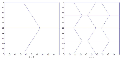
Figure 1: Ladder-shaped meshes for $\Omega=(0,1)\times(0,1)$.

	$h$	$k=0$		$k=1$		$k=2$
		Error	Rate	Error	Rate	Error	Rate
$\|\bm{q}-\bm{q}_{h}\|_{\bm{L}^{\infty}(\Omega)}$	$2^{-4}$	1.95E-01	-	2.84E-02	-	1.23E-03	-
	$2^{-5}$	9.38E-02	1.06	7.72E-02	1.88	1.30E-04	3.24
	$2^{-6}$	4.68E-02	1.00	1.98E-02	1.96	2.12E-05	2.62
	$2^{-7}$	2.33E-02	1.01	4.95E-02	2.00	2.65E-06	3.00
	$2^{-8}$	1.16E-02	1.01	1.23E-02	2.00	3.33E-07	2.99
$\|u-u_{h}\|_{L^{\infty}(\Omega)}$	$2^{-4}$	4.90E-02	-	4.96E-04	-	1.48E-04	-
	$2^{-5}$	1.41E-02	1.80	5.79E-05	3.10	1.22E-05	3.60
	$2^{-6}$	3.54E-03	1.99	6.96E-06	3.06	7.53E-07	4.02
	$2^{-7}$	8.88E-04	2.00	8.68E-07	3.00	4.80E-08	3.97
	$2^{-8}$	2.22E-04	2.00	1.08E-07	3.01	3.13E-09	3.94

Table 1: Example 1: $L^{\infty}(\Omega)$ errors for $\bm{q}_{h}$ and $u_{h}$ on domain $(0,1)\times(0,1)$ with Ladder-shaped meshes.

Example 2.

Next, we test the convergence rate of the $L^{\infty}$ norm estimate in 3D. The domain $\Omega=(0,1)\times(0,1)\times(0,1)$ and we use uniform simplex meshes. The exact solution $u(x,y,z)$ is chosen to be $u(x,y,z)=x(x-1)y(y-1)z(z-1)$. The source term $f$ is chosen to match the exact solution of (1.1) and the approximation errors are listed in Table 2. The rates match the theoretical predictions in Theorem 1.

	$h$	$k=0$		$k=1$		$k=2$
		Error	Rate	Error	Rate	Error	Rate
$\|\bm{q}-\bm{q}_{h}\|_{\bm{L}^{\infty}(\Omega)}$	$2^{-1}$	9.79E-03	-	6.47E-03	-	7.58E-03	-
	$2^{-2}$	8.61E-03	0.18	1.84E-03	1.81	1.49E-04	2.35
	$2^{-3}$	5.20E-03	0.73	5.01E-04	1.88	2.78E-05	2.42
	$2^{-4}$	2.77E-03	0.91	1.30E-04	1.94	4.18E-06	2.73
	$2^{-5}$	1.42E-03	0.96	3.36E-05	1.95	5.69E-07	2.88
$\|u-u_{h}\|_{L^{\infty}(\Omega)}$	$2^{-1}$	4.51E-03	-	9.86E-04	-	2.64E-04	-
	$2^{-2}$	1.31E-03	1.78	1.31E-04	2.90	1.65E-05	4.00
	$2^{-3}$	3.38E-04	1.96	1.73E-05	2.93	1.03E-07	4.00
	$2^{-4}$	8.51E-05	1.99	2.23E-06	2.96	6.44E-08	4.00
	$2^{-5}$	2.13E-05	2.00	2.92E-07	2.93	4.03E-09	4.00

Table 2: Example 2: $L^{\infty}(\Omega)$ errors for $\bm{q}_{h}$ and $u_{h}$ on domain $(0,1)\times(0,1)\times(0,1)$ with simplex meshes.

5 Conclusion

We have proved sharp $L^{\infty}$ norm estimates for the Poisson equation in both 2D and 3D. In the future, we would like to extend the results to some other models, such as the Stokes equation and Maxwell’s equations.

References

- [1] S. C. Brenner and L. R. Scott, The Mathematical Theory of Finite Element Methods, vol. 15 of Texts in Applied Mathematics, Springer, New York, third ed., 2008, https://doi.org/10.1007/978-0-387-75934-0, https://doi.org/10.1007/978-0-387-75934-0.
- [2] G. Chen, B. Cockburn, J. Singler, and Y. Zhang, Superconvergent interpolatory HDG methods for reaction diffusion equations I: An method, J. Sci. Comput., 81 (2019), pp. 2188–2212, https://doi.org/10.1007/s10915-019-01081-3.
- [3] G. Chen, P. Monk, and Y. Zhang, An HDG Method for the Time-dependent Drift–Diffusion Model of Semiconductor Devices, J. Sci. Comput., 80 (2019), pp. 420–443, https://doi.org/10.1007/s10915-019-00945-y.
- [4] G. Chen, P. B. Monk, and Y. Zhang, norm error estimates for HDG methods applied to the Poisson equation with an application to the Dirichlet boundary control problem, SIAM J. Numer. Anal., 59 (2021), pp. 720–745, https://doi.org/10.1137/20M1338551.
- [5] G. Chen, J. R. Singler, and Y. Zhang, An HDG method for Dirichlet boundary control of convection dominated diffusion PDEs, SIAM J. Numer. Anal., 57 (2019), pp. 1919–1946, https://doi.org/10.1137/18M1208708.
- [6] H. Chen, Pointwise error estimates of the local discontinuous Galerkin method for a second order elliptic problem, Math. Comp., 74 (2005), pp. 1097–1116, https://doi.org/10.1090/S0025-5718-04-01700-4.
- [7] H. Chen, Pointwise error estimates for finite element solutions of the Stokes problem, SIAM J. Numer. Anal., 44 (2006), pp. 1–28, https://doi.org/10.1137/S0036142903438100.
- [8] B. Cockburn, J. Gopalakrishnan, and R. Lazarov, Unified hybridization of discontinuous Galerkin, mixed, and continuous Galerkin methods for second order elliptic problems, SIAM J. Numer. Anal., 47 (2009), pp. 1319–1365, https://doi.org/10.1137/070706616.
- [9] B. Cockburn, J. Gopalakrishnan, and F.-J. Sayas, A projection-based error analysis of HDG methods, Math. Comp., 79 (2010), pp. 1351–1367, https://doi.org/10.1090/S0025-5718-10-02334-3.
- [10] Z. Dong and A. Ern, Hybrid high-order and weak galerkin methods for the biharmonic problem, arXiv preprint arXiv:2103.16404, (2021).
- [11] R. Durán, R. H. Nochetto, and J. P. Wang, Sharp maximum norm error estimates for finite element approximations of the Stokes problem in -D, Math. Comp., 51 (1988), pp. 491–506, https://doi.org/10.2307/2008760.
- [12] R. G. Durán, Error analysis in for mixed finite element methods for linear and quasi-linear elliptic problems, RAIRO Modél. Math. Anal. Numér., 22 (1988), pp. 371–387, https://doi.org/10.1051/m2an/1988220303711.
- [13] L. Gastaldi and R. Nochetto, Optimal -error estimates for nonconforming and mixed finite element methods of lowest order, Numer. Math., 50 (1987), pp. 587–611, https://doi.org/10.1007/BF01408578.
- [14] L. Gastaldi and R. H. Nochetto, Sharp maximum norm error estimates for general mixed finite element approximations to second order elliptic equations, RAIRO Modél. Math. Anal. Numér., 23 (1989), pp. 103–128, https://doi.org/10.1051/m2an/1989230101031.
- [15] V. Girault, R. H. Nochetto, and L. R. Scott, Max-norm estimates for Stokes and Navier-Stokes approximations in convex polyhedra, Numer. Math., 131 (2015), pp. 771–822, https://doi.org/10.1007/s00211-015-0707-8.
- [16] V. Girault, R. H. Nochetto, and R. Scott, Maximum-norm stability of the finite element Stokes projection, J. Math. Pures Appl. (9), 84 (2005), pp. 279–330, https://doi.org/10.1016/j.matpur.2004.09.017.
- [17] J. Guzmán, Local and pointwise error estimates of the local discontinuous Galerkin method applied to the Stokes problem, Math. Comp., 77 (2008), pp. 1293–1322, https://doi.org/10.1090/S0025-5718-08-02067-X.
- [18] J. Guzmán and D. Leykekhman, Pointwise error estimates of finite element approximations to the Stokes problem on convex polyhedra, Math. Comp., 81 (2012), pp. 1879–1902, https://doi.org/10.1090/S0025-5718-2012-02603-2.
- [19] W. Hu, J. Shen, J. R. Singler, Y. Zhang, and X. Zheng, A superconvergent hybridizable discontinuous Galerkin method for Dirichlet boundary control of elliptic PDEs, Numer. Math., 144 (2020), pp. 375–411, https://doi.org/10.1007/s00211-019-01090-2.
- [20] G. Kanschat and R. Rannacher, Local error analysis of the interior penalty discontinuous Galerkin method for second order elliptic problems, J. Numer. Math., 10 (2002), pp. 249–274, https://doi.org/10.1515/JNMA.2002.249.
- [21] O. A. Karakashian and F. Pascal, A posteriori error estimates for a discontinuous Galerkin approximation of second-order elliptic problems, SIAM J. Numer. Anal., 41 (2003), pp. 2374–2399, https://doi.org/10.1137/S0036142902405217, https://doi.org/10.1137/S0036142902405217.
- [22] C. Lehrenfeld, Hybrid Discontinuous Galerkin methods for solving incompressible flow problems, (2010). PhD Thesis.
- [23] P. Monk and Y. Zhang, An HDG method for the Steklov eigenvalue problem, IMA Journal of Numerical Analysis, (2021).
- [24] A. H. Schatz and L. B. Wahlbin, Interior maximum norm estimates for finite element methods, Math. Comp., 31 (1977), pp. 414–442, https://doi.org/10.2307/2006424.
- [25] A. H. Schatz and L. B. Wahlbin, On the quasi-optimality in of the -projection into finite element spaces, Math. Comp., 38 (1982), pp. 1–22, https://doi.org/10.2307/2007461.
- [26] A. H. Schatz and L. B. Wahlbin, Interior maximum-norm estimates for finite element methods. II, Math. Comp., 64 (1995), pp. 907–928, https://doi.org/10.2307/2153476.
- [27] R. Scholz, -convergence of saddle-point approximations for second order problems, RAIRO Anal. Numér., 11 (1977), pp. 209–216, 221, https://doi.org/10.1051/m2an/1977110202091.
- [28] R. Scott, Optimal estimates for the finite element method on irregular meshes, Math. Comp., 30 (1976), pp. 681–697, https://doi.org/10.2307/2005390.
- [29] J. Shen, J. R. Singler, and Y. Zhang, HDG-POD reduced order model of the heat equation, J. Comput. Appl. Math., 362 (2019), pp. 663–679, https://doi.org/10.1016/j.cam.2018.09.031.
- [30] Z. Shi and M. Wang, Finite Element Methods, vol. 58 of Series in Information and Computation Science, Science Press, Beijing, 2013.
- [31] J. P. Wang, Asymptotic expansions and -error estimates for mixed finite element methods for second order elliptic problems, Numer. Math., 55 (1989), pp. 401–430, https://doi.org/10.1007/BF01396046.