Methods for Creation and Linear Elastic Response Analysis of Packings of Semi-flexible Soft Polymer Chains

Abstract

From understanding the sand on the beach to the foam on your beer, soft sphere simulations have been crucial to the study of the amorphous world around us. However, many of the materials we interact with on a daily basis aren’t comprised of individual grains, but complex chains of polymers. By extending the soft sphere model to a model of chained spheres, we can learn more about the materials we interact with on a daily basis. In this methods paper, I show how one can find and study the physical properties of packings of flexible chains, rigid molecules, and everything in between. In addition to describing the energy landscape of these materials, these methods describe how to shear stabilize polymer packings, classify them in the jamming hierarchy, describe their elastic properties, and much more. This simple modification to soft sphere simulations has the potential to yield new discoveries surrounding glasses.

I Introduction

Glasses, grains, foams, sand, particulates, and colloidal suspensions are all examples of amorphous systems that undergo complicated phase transitions. These transitions have been studied extensively through simulations with packings of soft, athermal, frictionless spheres that interact through a one-sided contact potential. The success of this simplified model in furthering our understanding of glasses and jamming cannot be overstated Liu and Nagel (1998, 2010); Dagois-Bohy et al. (2012); Charbonneau et al. (2015, 2016); Lin et al. (2016); Morse and Corwin (2017); Dennis and Corwin (2020). However, many glassy systems are not comprised of soft spheres, but polymer chains that interact in more complex ways Ichihara et al. (1971); Cangialosi (2014); Monnier et al. (2021); Wu et al. (2021).

While the use of soft sphere packings will not and should not subside in the future, I hope we can get further understand glassy systems if we begin simulating packings of soft chains of spheres. I show how this can be done through a simple modification to code for soft sphere simulations.

The importance of polymer studies ranges from the biology of complex biomolecules such as proteins and chains of DNA Watson and Crick (1953); Boyer et al. (2011); Numata (2020) to the polyethylene that is omnipresent in our daily lives Royer et al. (2018); Ghatge et al. (2020). Packings of chains and polymers have been explored in experimental systems as well as in simulations Zou et al. (2009); Barrat et al. (2010); Karayiannis et al. (2012); Hoy (2017); Gartner and Jayaraman (2019); Mavrantzas (2021).

Here a novel method is proposed that can be more easily implemented and adapted to arbitrary cluster types and constraints. While real polymers are comprised of components joined by various types of interparticle forces, the work in this manuscript is done for the limiting case where the interparticle linkages are much stronger than the interaction potential between unlinked particles. The methods in this manuscript are focused specifically on soft chains of spheres which interact via a one-sided harmonic potential. However, the methods can be easily generalized to include more sophisticated interactions. Beyond the simple simulations of clusters of rigid molecules and flexible polymeric chains, one can also simulate clumping, aggregation, and the cementing of particles.

In this manuscript, I demonstrate how to create overjammed and critically jammed packings of arbitrarily defined semi-rigid clusters of spheres. It is further explained how these can be prepared and shear stabilized as well as describe how to find features of the packing, such as the normal modes, rattling clusters, classification in the jamming hierarchy, and elastic moduli. This simple extension to the already successful soft sphere packing model opens the door for many avenues of exploration in the physical properties of glassy systems.

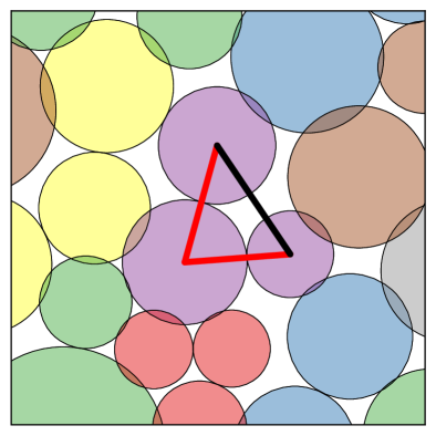
Figure 1: An example of a set of links in a packing. The red lines and the black line are all links, chosen to keep the purple cluster rigid. The red links join the particles together to form a cluster of three particles while the black link fixes the bond angle preventing the cluster from deforming. This rigid cluster only has three degrees of freedom: two translational and one rotational. However, three independent, unconstrained particles have six degrees of freedom. Adding the three links above effectively removes three degrees of freedom.

II Generating the Packings

Below a procedure is presented for generating packings of soft polymer chains that are force balanced in a local energy minimum through the use of constraints.

II.1 Generating Polymers: Links

The polymer packings are comprised of individual sets (or clusters) of spheres of variable radii, $r.$ The individual spheres in each cluster interact via a potential, $U,$ that is a function of their normalized overlaps, $\xi.$ To define these clusters, consider linkages between particles $i$ and $j$ of a fixed length. These are referred to as links.

By defining links, one is able to not only constrain the particles to be connected in arbitrary ways, but one can also fix the bond angles between particles. For example, given a triplet of circles, $a,\leavevmode\nobreak\ b,$ and $c$ connected via links $ab$ and $bc,$ the bond angle can be fixed by creating a link of some fixed length $l$ between $a$ and $c$ (see Figure 1).

II.2 The Orthonormalized Constraint Basis

Applying an arbitrary force to each of the particles in a packing would break their links and violate the constraints. The approach taken to prevent this is to project out the part of the force vector that violates the constraints to first order. Performing this projection will result in the forces that the chains actually experience and cause the appropriate cluster motions and torques in the simulation. Finding the projection requires finding an orthonormalized constraint basis.

In order to derive the orthonormal constraint basis, first consider the vector between two particles $i$ and $j$ that share a link, $\vec{x}_{ij}.$ Because we are working in periodic boundary conditions for arbitrary lattice vectors, I define the lattice vector matrix, $\Lambda,$ to be a $d\times d$ matrix where the columns are the lattice vectors. By considering a vector of integer lattice coordinates $\vec{z}_{ij}\in\mathbb{Z}^{d},$

$$x_{ij}^{\alpha}=x_{j}^{\alpha}-x_{i}^{\alpha}+\tensor{\Lambda}{{}^{\alpha}_{\gamma}}z_{ij}^{\gamma}$$ (1)

where $\alpha$ and $\gamma$ index the coordinates. It is also required that $\vec{z}_{ij}$ be an integer lattice vector which minimizes the norm of $x.$ For particles in contact, this means that $\vec{z}_{ij}$ is any integer vector that causes particle images $i$ and $j$ to be in contact. In general, this is degenerate, but without loss of generality, it can be asserted that every pair of overlapping spheres has exactly one $\vec{z}_{ij}$ and that $z_{ij}^{\alpha}\in\left\{-1,0,1\right\}$ for all coordinates $\alpha.$ If there is a link between particles $i$ and $j,$ our constraint is

$$c_{\langle ij\rangle}=\sqrt{\sum_{\alpha}\left(x_{ij}^{\alpha}\right)^{2}}-l_{\langle ij\rangle}=0$$ (2)

where $l_{\langle ij\rangle}$ is the constant length of bond $\langle ij\rangle.$ Defining

$$\hat{\tau}_{ij}^{\alpha}=\frac{x_{ij}^{\alpha}}{l_{\langle ij\rangle}}$$ (3)

to be the normalized distance vector between particles $i$ and $j,$ the constraint Jacobian is

$$\Omega_{k\alpha\langle ij\rangle}=\hat{\tau}_{ij}^{\alpha}\left(\delta_{jk}-\delta_{ik}\right)$$ (4)

such that the columns of this matrix are given by the derivatives of $c.$ If the packing does not contain degenerate links, then the constraint Jacobian has the property that the number of columns is equal to the rank. In practice, it is very easy to remove degenerate links, so to simplify computations and derivations, we assume there are no degenerate links.

This constraint Jacobian becomes very powerful in determining the forces on the unconstrained degrees of freedom. Because links in the same cluster share particles, the columns of this matrix will in general not be orthogonal. One can perform QR decomposition Trefethen and Bau (1997) on the constraint Jacobian to find an orthonormal basis for the constraints. QR decomposition can be fairly computationally intensive, so a parallelized modified Gram-Schmitt process is employed Kerr et al. (2009) on each of the clusters individually. Since no two independent clusters share degrees of freedom, their columns will be automatically orthogonal. After performing the decomposition on our constraint Jacobian, the orthonormalized constraint basis, $\Omega_{\textrm{o}}$ is found. This matrix can be used to constrain the forces applied to the packing. Given an arbitrary force vector, $\vec{F},$ which acts on the particle positions, one can project out the part of the vector that lies along the constraints. This projection gives the constrained force vector:

$$\vec{F}_{\textrm{cons}} =\vec{F}-\Omega_{\textrm{o}}\Omega_{\textrm{o}}^{T}\vec{F}$$ (5)

$$=\left(\mathbf{1}-\Omega_{\textrm{o}}\Omega_{\textrm{o}}^{T}\right)\vec{F}.$$ (6)

For a system of rigid clusters, this constrained force removes the need to consider torques as it performs the correct angular rotation to first order. Similarly, for clusters with free bond angles, this alters the bond angles appropriately. It is worth noting that equation 6 does not apply only to forces, but other variables as well. For example, one can find a constrained velocity in the same manner.

II.3 Higher Order Corrections

The previously described constraint method is only correct for infinitesimal perturbations. As the goal is to perform a quench on these clusters, the non-linear contributions will accumulate over the course of the simulation causing our constraints to be violated. To combat this, the constraints are periodically reaffixed. This can be achieved numerically by employing the Newton-Rhapson method Verbeke and Cools (1995). For simplicity, consider the positions of the particles to be encapsulated by a single vector, $\vec{x}.$ Practically, this can be achieved by simply flattening the matrix of positions. If the constraints are considered to be a vector, then the following recursive equation can be solved iteratively:

$$\Omega^{T}(\vec{x}_{k})\left[\vec{x}_{k+1}-\vec{x}_{k}\right]=-\vec{c}(\vec{x}_{k})$$ (7)

for $\vec{x}_{k+1}$ where $k$ represents the iteration number. This equation can be solved using a method such as Gaussian elimination Trefethen and Bau (1997). This algorithm is continued until iteration $n$ where $\left|\vec{c}(\vec{x}_{n})\right|<p$ for the desired precision $p.$ When starting in a position that is very close to satisfying the constraints, this algorithm should terminate after just a few steps.

This now fully defines a method for generating semi-flexible soft polymer packings, however if one also wants to probe the linear elastic response, they should do so for packings that are stable with respect to strains.

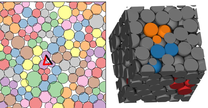
Figure 2: Polymer packings made up of $50$ clusters of three particles with fixed bond angles in 2D (left) and 3D (right). For visualization purposes, only three of the rigid clusters are shown in the three dimensional packing.

II.4 Shear Stabilization

While true stress-strain isotropy is typically reserved only for certain perfect crystalline packings, the amorphous nature of large thermal systems of grains and polymers causes them to be approximately isotropic as well. However, this is only true if they are shear stabilized. That is, if the packing is not at a minimum with respect to all strain degrees of freedom, then there exists a strain which when applied causes the energy of the packing to decrease. This violates the isotropic assumption which means that the packings cannot be described with elastic moduli. While plenty of excellent research has been done on elastic response in systems which are not shear stabilized Liao et al. (1997); Manning (2011); Manning and Liu (2011); Banigan et al. (2013); Rainone et al. (2020), the desire for shear stabilization is often warranted nonetheless Donev et al. (2004a); Dagois-Bohy et al. (2012).

Shear stabilization is achieved by minimizing the energy of a packing with respect to both position and strain degrees of freedom. In other words, we also consider the packing’s lattice vectors to be subject to change. Given the position of a node, $\vec{p}_{0},$ one can describe its lattice images as

$$\vec{p}=\vec{p}_{0}+\Lambda\vec{z}.$$ (8)

A perturbation of the lattice vectors, $\Delta\Lambda,$ results in

$$\Delta\vec{p}=\left(\Delta\Lambda\right)\vec{z}.$$ (9)

Solving equation 8 for $\vec{z}$ and making a substitution,

$$\Delta\vec{p}=\left(\Delta\Lambda\right)\Lambda^{-1}\left(\vec{p}-\vec{p}_{0}\right).$$ (10)

Therefore, from the definition of the strain matrix,

$$\mathbf{\varepsilon}\equiv\nabla_{\vec{p}}\left(\Delta\vec{p}\right)=\left(\Delta\Lambda\right)\Lambda^{-1}.$$ (11)

It’s also important to notice that the strain matrix must be symmetric; this can be achieved by defining it’s derivatives as

$$\frac{\partial\mathbf{\varepsilon}_{ij}}{\partial\mathbf{\varepsilon}_{kl}}\equiv\frac{1}{2}\left(\delta_{ik}\delta_{jl}+\delta_{il}\delta_{jk}\right).$$ (12)

It is crucial that the positions of particles be a function of the affine strain, so one can then find the distance between particle $i$ and $j$ as a function of position and strain,

$$\psi_{ij}^{\alpha}=\left(\tensor{\delta}{{}^{\alpha}_{\beta}}+\tensor{\varepsilon}{{}^{\alpha}_{\beta}}\right)\left(x_{j}^{\beta}-x_{i}^{\beta}+\tensor{\Lambda}{{}^{\beta}_{\gamma}}z_{ij}^{\gamma}\right).$$ (13)

The constraints, $c_{\langle ij\rangle},$ and constraint Jacobian, $\Omega,$ can also be redefined as functions of the strain degrees of freedom. This means that

$$c_{\langle ij\rangle}(\varepsilon)=\sqrt{\sum_{\alpha}\left(\psi_{ij}^{\alpha}(\varepsilon)\right)^{2}}-l_{\langle ij\rangle}.$$ (14)

The columns of $\Omega$ are comprised of derivatives of the constraints with respect to all of the degrees of freedom, positional and strain. The derivatives are evaluated at the current positions of the particles and the current strain of the packing. Because the positions and lattice vectors are updated at every step of the minimization protocol, the constraint derivates can be evaluated at zero strain. One can derive that

$$\frac{\partial c_{\langle ij\rangle}}{\partial x_{k}^{\alpha}}\bigg{|}_{\varepsilon=0}=\hat{\tau}_{ij}^{\alpha}\left(\delta_{jk}-\delta_{ik}\right)$$ (15)

as before. However,

$$\frac{\partial c_{\langle ij\rangle}}{\partial\tensor{\varepsilon}{{}^{a}_{b}}}\bigg{|}_{\varepsilon=0}=\hat{\tau}_{ij}^{a}\hat{\tau}_{ij}^{b}l_{\langle ij\rangle}$$ (16)

after employing equation 12. It’s important to note that all of the columns of our constraint Jacobian are linearly dependent which prevents the QR decomposition algorithm from taking advantage of the speed increase gained by assuming that the constraints between different clusters are orthogonal.

As the strain tensor is required to be a $d\times d$ symmetric matrix, there are $d(d+1)/2$ strain degrees of freedom. However, there is one final constraint to consider for shear stabilizing a packing of polymers: constraining the box volume. For a packing of monomers where the box volume is not constrained, the strain forces will always lead to the decompression of the box causing an unjamming event. It is therefore required that the applied strains keep the box volume constant. For infinitesimal strains, this constraint is simply $\operatorname{Tr}(\varepsilon)=0$ Torquato et al. (2003); Donev et al. (2004a, b). The derivative of this constraint with respect to positional degrees of freedom is zero, but for the strain degrees of freedom, this means that

$$\frac{\partial}{\partial\tensor{\varepsilon}{{}^{a}_{b}}}\left(\sum_{\alpha}\tensor{\varepsilon}{{}^{\alpha}_{\alpha}}\right)=\delta_{ab}.$$ (17)

To avoid confusion, the constraint Jacobian is referred to as $\Omega$ if it only involves positional degrees of freedom and $\Gamma$ if it involves both positional and strain degrees of freedom as well as the volume preserving constraint. Likewise, the othornormalized versions are called $\Omega_{o}$ and $\Gamma_{o}$ respectively. Just as in equation 6, given an arbitrary force vector that involves the derivatives of positions and strain, $\vec{F},$ the constrained force is given by

$$\vec{F}_{\textrm{cons}}=\left(\mathbf{1}-\Gamma_{o}\Gamma_{o}^{T}\right)\vec{F}.$$ (18)

II.5 Performing Minimization

The constraints described above can be applied to any minimization algorithm that involves forces, such as gradient descent and FIRE Bitzek et al. (2006) as well as molecular dynamics simulations. While this algorithm can be realized with any potential, I choose to direct my attention to a soft sphere potential of the form,

$$U(x,\varepsilon)=\frac{1}{2w}\sum_{i}\sum_{j\in\partial i}\left(\xi_{ij}\right)^{w}$$ (19)

where $w$ is some power and $\xi_{ij}$ is the normalized overlap,

$$\xi_{ij}=1-\frac{\rho_{ij}}{\sigma_{ij}}.$$ (20)

In this equation $\rho_{ij}=\sqrt{\sum_{\alpha}\left(\psi_{ij}^{\alpha}\right)^{2}},$ $\sigma_{ij}$ is the sum of the radii, and $j\in\partial i$ are defined to be those particles $j$ which are in contact with particle $i.$ This is understood to be a one-sided potential meaning that particles which are not overlapping do not interact. As a result, the contact network of our polymers changes throughout the minimization.

The positional forces are unchanged,

$$F_{x,k}^{\mu}=-\frac{\partial U}{\partial x_{k}^{\mu}}\bigg{|}_{\varepsilon=0}=\sum_{i\in\partial k}\xi_{ik}^{w-1}\frac{\hat{n}_{ik}^{\mu}}{\sigma_{ik}}$$ (21)

and the strain forces are

$$F_{\varepsilon,ab}=-\frac{\partial U}{\partial\tensor{\varepsilon}{{}^{a}_{b}}}\bigg{|}_{\varepsilon=0}=\frac{1}{2}\sum_{i}\sum_{j\in\partial i}\frac{\rho_{ij}}{\sigma_{ij}}\xi_{ij}^{w-1}\hat{n}_{ij}^{a}\hat{n}_{ij}^{b}$$ (22)

where $\hat{n}_{ij}^{a}$ is the normalized contact vector between particles $i$ and $j$ where $a$ indexes the coordinates.

Now all that is left to do is to apply constraints to these forces and perform the minimization. After each minimization step, the positions and strains are updated. To simplify the scheme, the particle perturbations are applied first then the affine strain perturbs the particles further. The strain to our lattice vectors is also applied such that

$$\Lambda_{\textrm{new}}=\left(\mathbf{1}+\varepsilon\right)\Lambda.$$ (23)

Finally, the strain is reset to zero. However, applying a finite strain to the lattice vectors will only preserve the volume to first order. To correct this, the lattice vectors are uniformly rescaled after each step so that they have a determinant of one. The polymer constraints also become violated to higher order so the same scheme that appears in section II.3 must be applied with our updated lattice vectors. To demonstrate the success of this methodology, two and three dimensional minimized system with $50$ rigid clusters each containing three particles is shown in Figure 2.

II.6 Crossing Links, Rattling clusters, and Danglers

Careful initialization of two dimensional packings is important to avoid crossing links. If two dimers have links that cross, as seen in Figure 3, this forms a stable configuration that minimization will not affect. This behavior can occur between different clusters or even in a single cluster of adequate length. To avoid this behavior, one can initialize the system such that link crossings are forbidden prior to minimization. However, if large overlaps are present in a configuration prior to minimization, link crossings may still occur. This behavior becomes more likely for larger timesteps in the beginning of the quench.

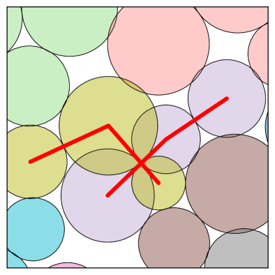
Figure 3: Two clusters and their links are shown in a packing of short chains. Two of the red links were crossing before minimization and these two links remain crossing after the minimization is finished. These two chains are in force balance despite being in a high energy configuration. This only occurs in two dimensions and can be mitigated by ensuring that there are no crossing links before beginning the quench.

In a system of monomers at densities close to jamming, particles which are not locally constrained, termed rattlers, may introduce zero energy eigenmodes, or floppy modes, to the system. Rattlers are particles that are able to move independently of the other particles without affecting the system’s energy. Polymer chain systems analogously can have rattling clusters. A rattling cluster is a cluster in which a subset of the cluster can move independently of the other clusters without affecting the system’s energy. A particular type of rattling cluster that may appear is a dangler. A dangler is a single particle that does not interact with the other particles except by it’s link (see Figure 4).

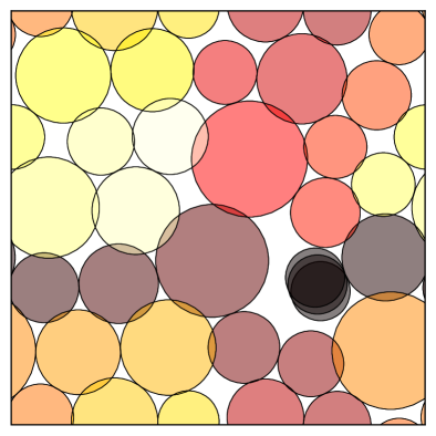
Figure 4: A chain of 30 particles in force balance. This chain is an example of a rattling cluster because one end of the chain (black) is constrained by its link, but still has a degree of freedom to move (as shown). This free motion is a floppy mode and this means that the packing is not collectively jammed. However, simply removing the end of the chain will remove this floppy mode from the system, leaving a subsystem that is collectively jammed.

III Finding Critically Jammed Systems

A critically jammed packing is a packing that is rigid and has zero energy. To create such a polymer packing, start with randomly distributed cluster positions and bond angles (avoiding link crossings in 2D) at a density which is much higher than the expected jamming density. These clusters are allowed to interact via a harmonic contact potential and the energy is minimized with the FIRE algorithm. The size of each cluster and the corresponding constraints are then uniformly decreased while maintaining their average positions. After minimizing this lower-density packing, the process is repeated until the energy reaches a low threshold. The amount by which the packing fraction is decreased at each step is decided by taking advantage of the scaling relationship between energy and distance to the jamming density for soft sphere systems, $\phi-\phi_{j},$ given in reference Charbonneau et al. (2015).

Because of the aforementioned rattling clusters, packings prepared in this manner will typically have some form of floppy mode present. This effect will be discussed in section V.

IV Defining the constrained Hessian and Rigidity Matrices

IV.1 The Constrained Hessian

For a packing of polymers, one may wish to find the normal modes, with or without strain degrees of freedom. In order to do that, one must first find the second derivatives of the energy function with respect to these degrees of freedom. These are as follows,

$$H_{xx}=\left.\frac{\partial^{2}U}{\partial r_{j}^{\nu}\partial r_{k}^{\mu}}\right|_{\varepsilon=0}=$$ (24)

$$\delta_{kj}\sum_{i\in\partial k}\left[\left(w-1\right)\frac{\xi_{ik}^{w-2}}{\sigma_{ik}^{2}}n_{ik}^{\mu}n_{ik}^{\nu}+\frac{\xi_{ik}^{w-1}}{\rho_{ik}\sigma_{ik}}(n_{ik}^{\mu}n_{ik}^{\nu}-\delta^{\mu\nu})\right]$$

$$-\delta_{\langle kj\rangle}\left[\left(w-1\right)\frac{\xi_{kj}^{w-2}}{\sigma_{kj}^{2}}n_{kj}^{\mu}n_{kj}^{\nu}+\frac{\xi_{kj}^{w-1}}{\rho_{kj}\sigma_{kj}}(n_{kj}^{\mu}n_{kj}^{\nu}-\delta^{\mu\nu})\right],$$

$$H_{\varepsilon x}=\left.\frac{\partial^{2}U}{\partial\tensor{\varepsilon}{{}^{a}_{b}}\partial r_{k}^{\mu}}\right|_{\varepsilon=0}=$$ (25)

$$\sum_{i}\frac{\delta_{\langle ik\rangle}}{\sigma_{ik}}\biggl{\{}\left[\left(w-1\right)\xi_{ik}^{w-2}-\left(w-2\right)\xi_{ik}^{w-1}\right]n_{ik}^{\mu}n_{ik}^{\kappa}n_{ik}^{\beta}\biggr{.}$$

$$\biggl{.}-\xi_{ik}^{w-1}\left(\delta^{\beta\mu}n_{ik}^{\kappa}+\delta^{\mu\kappa}n_{ik}^{\beta}\right)\biggr{\}}\left(\frac{\partial\tensor{\varepsilon}{{}^{\kappa}_{\beta}}}{\partial\tensor{\varepsilon}{{}^{a}_{b}}}\right),$$

and

$$H_{\varepsilon\varepsilon}=\left.\frac{\partial^{2}U}{\partial\tensor{\varepsilon}{{}^{g}_{h}}\partial\tensor{\varepsilon}{{}^{a}_{b}}}\right|_{\varepsilon=0}=$$ (26)

$$\frac{1}{2}\sum_{i}\sum_{j\in\partial i}\left(1-\xi_{ij}\right)\biggl{\{}\left[\left(w-1\right)\xi_{ij}^{w-2}-\left(w-2\right)\xi_{ij}^{w-1}\right]n_{ij}^{\alpha}n_{ij}^{\mu}\biggr{.}$$

$$\biggl{.}-\xi_{ij}^{w-1}\delta^{\alpha\mu}\biggr{\}}n_{ij}^{\beta}n_{ij}^{\nu}\left(\frac{\partial\tensor{\varepsilon}{{}^{\mu}_{\nu}}}{\partial\tensor{\varepsilon}{{}^{g}_{h}}}\right)\left(\frac{\partial\tensor{\varepsilon}{{}^{\alpha}_{\beta}}}{\partial\tensor{\varepsilon}{{}^{a}_{b}}}\right).$$

In these equations, the term $\delta_{\langle km\rangle}$ is equal to one if particles $k$ and $m$ are in contact and zero otherwise. These terms can be combined to find the extended hessian, which is the second derivative of the energy function in terms of both positional and strain degrees of freedom:

$$H_{0}=\begin{pmatrix}H_{xx}&H_{x\varepsilon}\\ H_{x\varepsilon}^{T}&H_{\varepsilon\varepsilon}\end{pmatrix}.$$ (27)

The extended hessian can be used to find the energy of a perturbation that is done to the positions of individual particles and the strains. However, with polymer packings, we do not have access to all of these degrees of freedom. If there are $N$ particles in $d$ dimensions with $N_{l}$ nondegenerate links, the extended hessian will have $Nd+d(d+1)/2$ rows and columns whereas there are actually $N_{\textrm{dof}}=Nd+d(d+1)/2-N_{l}-1$ degrees of freedom (where the constraints due to the links and the volume-preserving strain have been subtracted). In order to calculate the energy of a perturbation and the normal modes of the polymer packing, one needs to translate the perturbations of the particles and affine strains to some basis of the true degrees of freedom. This can be achieved by performing a change of basis from the original basis to a basis of the true degrees of freedom and the constraints.

Let $\vec{y}$ be a vector of length $Nd+d(d+1)/2$ that contains the position and strain variables, let $\vec{y}_{t}$ be a vector of length $N_{\textrm{dof}}$ that contains the true degrees of freedom, and let $\vec{\lambda}$ be a vector of length $N_{l}+1$ corresponding to the constraint degrees of freedom. We need a square matrix, $Q,$ that decomposes $\vec{y}$ into $\vec{y}_{t}$ and $\vec{\lambda}$ such that

$$\begin{pmatrix}\vec{\lambda}\\ \vec{y}_{t}\end{pmatrix}=Q^{T}\vec{y}.$$ (28)

Without loss of generality, one can define a matrix,

$$\begin{pmatrix}\Gamma&\mathrm{Null}(\Gamma^{T})\end{pmatrix}.$$ (29)

This gives a non-singular matrix where the first $N_{l}+1$ columns correspond to our constraints. This matrix can then be subjected to QR decomposition to give a matrix $Q.$

With this new matrix, $Q,$ one can define a rectangular change of basis matrix as

$$B=\begin{pmatrix}\mathbf{0}_{N_{l}+1}&\mathbf{1}_{N_{\textrm{dof}}}\end{pmatrix}Q^{T}$$ (30)

such that

$$\vec{y}_{t}=B\vec{y}.$$ (31)

This basis is also useful for removing the components of a vector $\vec{y}$ that violate our constraints:

$$\vec{y}^{\prime}=B^{T}B\vec{y}.$$ (32)

With this matrix, $B,$ the constrained extended hessian becomes

$$H_{\textrm{E}}=BH_{0}B^{T}.$$ (33)

Given some perturbation, $\vec{y}_{t}$ of our $N_{\textrm{dof}}$ degrees of freedom, the change in energy can be computed as

$$\Delta E=\frac{1}{2}\vec{y}_{t}^{T}H_{\textrm{E}}\vec{y}_{t}.$$ (34)

The extended hessian can also be diagonalized to find the normal modes. The only problem is that the normal modes are in terms of a rather confusing basis, but this can be easily rectified by taking the matrix of eigenvectors and multiplying them by $B^{T}$ giving a set of $N_{\textrm{dof}}$ eigenmodes in the familiar basis of positions of particles and strains. This entire procedure can also be easily adapted to use the matrix, $\Omega,$ and create an extended hessian that deals only with positional degrees of freedom.

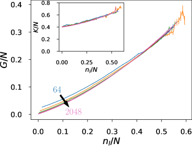
Figure 5: The shear and bulk (inset) moduli of three dimensional packings of clustered particles. Starting with shear stabilized, critically jammed systems of monomers, links are randomly added to the contact network and bond angles are frozen to simulate cementing events. The number of links at any given point is $n_{l}$ and this does not include those links which are added to fix the bond angles. There are about $25$ packings for each $N$ (from $2^{6}$ to $2^{1}1$) in which $50$ independent percolation experiments were performed. The data for each $N$ and $n_{l}$ was subject to a weighted average where the Reuss and Voigt averages were used as a minimum and maximum respectively. The error bars show the weighted standard error.

IV.2 The Constrained Rigidity Matrix

If one wanted to examine the underlying unnormalized, unstressed spring network of a packing and find the states of self stress, they could define the extended rigidity matrix. The rigidity matrix relates perturbations to bond stresses, so to derive it, consider the effect that perturbing or straining the packing has on the bond stresses. For particle perturbations, the rigidity matrix has the form

$$R_{x,\langle ij\rangle\left(k\gamma\right)}=\left(\delta_{jk}-\delta_{ik}\right)n_{ij}^{\gamma}.$$ (35)

For strains, the rigidity matrix has the form

$$R_{\varepsilon,\langle ij\rangle\left(k\gamma\right)}=n_{ij}^{\alpha}n_{ij}^{\beta}\sigma_{ij}.$$ (36)

These two terms can be combined to get the rigidity matrix in terms of strains and positions,

$$R_{0,\langle ij\rangle}=\begin{pmatrix}R_{x,\langle ij\rangle}&R_{\varepsilon,\langle ij\rangle}\end{pmatrix}$$ (37)

such that for a vector $\vec{y}=\begin{pmatrix}\vec{x}\\ \vec{\varepsilon}\end{pmatrix},$

$$R_{0,\langle ij\rangle}\vec{y}=R_{x,\langle ij\rangle}\vec{x}+R_{\varepsilon,\langle ij\rangle}\vec{\varepsilon}.$$ (38)

As before, one can perform a change of basis on this rigidity matrix to find the constrained extended rigidity matrix,

$$R_{\textrm{E}}=R_{0}B^{T}.$$ (39)

Note that the constrained extended rigidity matrix is only defined for the bonds in the system, not for the links. If the links were included, then $R_{\textrm{E}}$ would return zero stress on those bonds regardless of the choice for $\vec{y}_{t}.$

Similarly, the states of self stress for the network are the left singular vectors that have a zero singular value. The constrained extended $\mathcal{N}$-matrix can be computed as $\mathcal{N}_{\textrm{E}}=R_{\textrm{E}}R_{\textrm{E}}^{T}$ and the constrained extended dynamical matrix as $\mathcal{D}_{\textrm{E}}=R_{\textrm{E}}^{T}R_{\textrm{E}}$ for the underlying unstressed spring network.

V Testing for strict jamming

If one were to make a hard sphere polymer packing, such as those found by following the procedure described in section III, one might want to know whether or not this packing remains stable against all possible combinations of strains and perturbations. One way to do this is to employ a linear programming algorithm based on the one found in reference Donev et al. (2004b) with the constrained extended rigidity matrix in place of the adjacency matrix. The linear program is:

$$\textrm{min\leavevmode\nobreak\ }\vec{b}^{T}\vec{y}_{t}$$ (40)

such that $$R_{\textrm{E}}\vec{y}_{t}\leq\vec{0}$$ (41)

where $$\left|\vec{y}_{t}\right|\leq y_{\textrm{max}}.$$ (42)

In this program, we are looking for the vector $\vec{y}_{t}$ which is subjected to some random load vector $\vec{b}$ that is bounded such that the length is less than some finite value $y_{\textrm{max}}.$ If this algorithm returns a nonzero vector, $\vec{y}_{t},$ then $\vec{y}_{t}$ describes an unjamming motion. Because of the presence of rattling clusters, this may be the case. To determine which particles are contributing to the nonzero $\vec{y}_{t},$ one can find the nonzero indices for $B^{T}\vec{y}_{t}.$ Those rattling clusters should be removed from the packing before the linear program is executed again. This process can be repeating until $\vec{y}_{t}=\vec{0}$ is found. One must also run the same linear program for $\textrm{min\leavevmode\nobreak\ }-\vec{b}^{T}\vec{y}_{t}$ to ensure that the polymer subpacking is strictly jammed Donev et al. (2004b). As in the previous sections, the strain degrees of freedom do not need to be added; the same process can be adapted to $R_{x}$ to test for collective jamming.

VI Computing the Compliance Matrix

Now that jamming and normal modes for the polymer systems have been discussed, the discussion can conclude by computing the elastic moduli. To compute the elastic moduli, the compliance matrix, $S,$ is computed. This matrix relates the stress to the strain,

$$\vec{\varepsilon}=S\vec{\sigma}.$$ (43)

Before this is derived, consider Hooke’s law for the unconstrained extended hessian,

$$H_{0}\begin{pmatrix}\Delta\vec{x}\\ \vec{\varepsilon}\end{pmatrix}=\begin{pmatrix}-\vec{F}\\ \vec{\sigma}\end{pmatrix}.$$ (44)

Applying an arbitrary strain, $\vec{\varepsilon},$ and perturbation, $\Delta\vec{x},$ puts a stress, $\vec{\sigma},$ and interparticle forces, $\vec{F},$ on our packing. Not every combination of $\Delta\vec{x}$ and $\vec{\varepsilon}$ is allowed, so we need to project out the part of our vector that violates the constraints. From equation 32 one can achieve this with $B^{T}B.$ However, this is not quite correct. When finding the elastic moduli, deformations which may affect the volume of the packing are allowed. As such, $B$ is rederived with the volume-conserving constraint excluded from $\Gamma.$ This new rectangular change of basis is referred to as $B_{-1}.$ A new constrained hessian can be defined as

$$H_{c}=B_{-1}^{T}B_{-1}H_{0}B_{-1}^{T}B_{-1}$$ (45)

such that it contains the same degrees of freedom as the original hessian.

To find the stress-strain relationship, it is not enough to apply an affine strain. Simply applying an affine strain will cause the packing to lose force balance. When the stress-strain relationship is probed in granular packings, minimization steps are taken between strain steps. What one must do is apply an arbitrary affine strain and a corresponding nonaffine perturbation, $\Delta\vec{x}_{\textrm{na}},$ such that force balance is kept. For an unconstrained hessian, Hooke’s law can be applied to achieve an equation such as the following:

$$H_{0}\begin{pmatrix}\Delta\vec{x}_{\textrm{na}}\\ \vec{\varepsilon}\end{pmatrix}=\begin{pmatrix}\vec{0}\\ \vec{\sigma}\end{pmatrix}.$$ (46)

However, for the constrained hessian, this relationship is false. To understand why, imagine applying a particular perturbation and strain that strictly violate our constraints; this would result in zero strain. This is the exact opposite of what one would expect. It should be impossible to apply such a perturbation and strain, therefore one would expect the result of such a test to return an infinite stress. This is easily remedied by taking the Moore-Penrose pseudoinverse ben (2003) of $H_{c}.$ This works because the pseudoinverse preserves all of the zero eigenvalues. We can then conclude that

$$\left(H_{c}\right)^{-1}\begin{pmatrix}\vec{0}\\ \vec{\sigma}\end{pmatrix}=\begin{pmatrix}\Delta\vec{x}_{\textrm{na}}\\ \vec{\varepsilon}\end{pmatrix}.$$ (47)

This is much easier to understand as well because while certain strains may not be possible, any stress is allowed. The result will never violate our constraints, but may lead to zero strain. If $\left(H_{c}\right)^{-1}$ is partitioned,

$$\vec{\varepsilon}=S\vec{\sigma}$$ (48)

where

$$S=\begin{pmatrix}\mathbf{0}_{Nd\times Nd}&\mathbf{0}_{Nd\times s}\\ \mathbf{0}_{s\times Nd}&\mathbf{1}_{s\times s}\end{pmatrix}\left(H_{c}\right)^{-1}$$ (49)

is the compliance matrix.

For three dimensional polymer chain systems, the shear and bulk moduli can be found from the Voigt, Reuss, and Hill averages under the assumption that the configuration is nearly isotropic Hill (1952); Watt et al. (1976). From these averages, the poisson ratio and anisotropy can also be calculated. To understand this procedure, take three dimensional shear stabilized systems of monodisperse monomers at a single state of self stress and randomly replace some of their contacts with links. At a certain point sufficiently many links are added to prevent certain stresses from causing strains. These impossible stresses show up as zero modes in the compliance matrix and indicate a direction in which the shear modulus is infinite. Adding additional links will also eventually cause the compliance matrix to become zero, indicating a completely rigid packing of polymer chains. The bulk and shear moduli for these systems as a function of the fraction of added links, $n_{l}/N,$ (not including those added to preserve bond angles) are shown in Figure 5.

VII Conclusions

In this methods paper I have discussed how to generate packings of arbitrarily defined polymer chains. I described how to simulate the annealing of these packings and how they can be shear stabilized in the process. I gave examples of undesirable behaviors and how to prevent them as well as the definitions of rattling clusters and danglers. I then explained how to find the normal modes, classification in the jamming hierarchy, and elastic moduli. This work lays the foundations for a more thorough exploration of the mechanical properties of packings of polymer chains and molecules as well as a clear method for furthering our understanding of many important topics such as the polymer glass transition, clumping, and cementing events.

VIII Acknowledgments

I thank Eric Corwin, James Sartor, and Heinrich Jaeger for helpful discussions and feedback. This work was supported by National Science Foundation (NSF) Career Award DMR-1255370 and the Simons Foundation No. 454939.

References

- Liu and Nagel (1998) Andrea J. Liu and Sidney R. Nagel, “Jamming is not just cool any more,” Nature 396, 21–22 (1998), number: 6706 Publisher: Nature Publishing Group.
- Liu and Nagel (2010) Andrea J. Liu and Sidney R. Nagel, “The Jamming Transition and the Marginally Jammed Solid,” Annual Review of Condensed Matter Physics 1, 347–369 (2010), publisher: Annual Reviews.
- Dagois-Bohy et al. (2012) Simon Dagois-Bohy, Brian P. Tighe, Johannes Simon, Silke Henkes, and Martin van Hecke, “Soft-Sphere Packings at Finite Pressure but Unstable to Shear,” Physical Review Letters 109, 095703 (2012), publisher: American Physical Society.
- Charbonneau et al. (2015) Patrick Charbonneau, Eric I. Corwin, Giorgio Parisi, and Francesco Zamponi, “Jamming Criticality Revealed by Removing Localized Buckling Excitations,” Physical Review Letters 114, 125504 (2015), publisher: American Physical Society.
- Charbonneau et al. (2016) Patrick Charbonneau, Eric I. Corwin, Giorgio Parisi, Alexis Poncet, and Francesco Zamponi, “Universal Non-Debye Scaling in the Density of States of Amorphous Solids,” Physical Review Letters 117, 045503 (2016), publisher: American Physical Society.
- Lin et al. (2016) Jie Lin, Ivane Jorjadze, Lea-Laetitia Pontani, Matthieu Wyart, and Jasna Brujic, “Evidence for Marginal Stability in Emulsions,” Physical Review Letters 117, 208001 (2016), publisher: American Physical Society.
- Morse and Corwin (2017) Peter K. Morse and Eric I. Corwin, “Echoes of the Glass Transition in Athermal Soft Spheres,” Physical Review Letters 119, 118003 (2017), publisher: American Physical Society.
- Dennis and Corwin (2020) R. C. Dennis and E. I. Corwin, “Jamming Energy Landscape is Hierarchical and Ultrametric,” Physical Review Letters 124, 078002 (2020), publisher: American Physical Society.
- Ichihara et al. (1971) Shoji Ichihara, Akihiko Komatsu, Yoshiharu Tsujita, Takuhei Nose, and Toshio Hata, “Thermodynamic Studies on the Glass Transition and the Glassy State of Polymers. I. Pressure Dependence of the Glass Transition Temperature and Its Relation to Other Thermodynamic Properties of Polystyrene,” Polymer Journal 2, 530–534 (1971), bandiera_abtest: a Cg_type: Nature Research Journals Number: 4 Primary_atype: Research Publisher: Nature Publishing Group.
- Cangialosi (2014) D. Cangialosi, “Dynamics and thermodynamics of polymer glasses,” Journal of Physics. Condensed Matter: An Institute of Physics Journal 26, 153101 (2014).
- Monnier et al. (2021) Xavier Monnier, Juan Colmenero, Marcel Wolf, and Daniele Cangialosi, “Reaching the Ideal Glass in Polymer Spheres: Thermodynamics and Vibrational Density of States,” Physical Review Letters 126, 118004 (2021), publisher: American Physical Society.
- Wu et al. (2021) Guozhang Wu, Yuanbiao Liu, and Gaopeng Shi, “New Experimental Evidence for Thermodynamic Links to the Kinetic Fragility of Glass-Forming Polymers,” Macromolecules 54, 5595–5606 (2021), publisher: American Chemical Society.
- Watson and Crick (1953) J. D. Watson and F. H. C. Crick, “Molecular Structure of Nucleic Acids: A Structure for Deoxyribose Nucleic Acid,” Nature 171, 737–738 (1953), bandiera_abtest: a Cg_type: Nature Research Journals Number: 4356 Primary_atype: Research Publisher: Nature Publishing Group.
- Boyer et al. (2011) Cyrille Boyer, Xin Huang, Michael R. Whittaker, Volga Bulmus, and Thomas P. Davis, “An overview of protein–polymer particles,” Soft Matter 7, 1599–1614 (2011), publisher: The Royal Society of Chemistry.
- Numata (2020) Keiji Numata, “How to define and study structural proteins as biopolymer materials,” Polymer Journal 52, 1043–1056 (2020), bandiera_abtest: a Cc_license_type: cc_by Cg_type: Nature Research Journals Number: 9 Primary_atype: Reviews Publisher: Nature Publishing Group Subject_term: Biomaterials – proteins;Polymers Subject_term_id: biomaterials-proteins;polymers.
- Royer et al. (2018) Sarah-Jeanne Royer, Sara Ferrón, Samuel T. Wilson, and David M. Karl, “Production of methane and ethylene from plastic in the environment,” PLoS ONE 13, e0200574 (2018).
- Ghatge et al. (2020) Sunil Ghatge, Youri Yang, Jae-Hyung Ahn, and Hor-Gil Hur, “Biodegradation of polyethylene: a brief review,” Applied Biological Chemistry 63, 27 (2020).
- Zou et al. (2009) Ling-Nan Zou, Xiang Cheng, Mark L. Rivers, Heinrich M. Jaeger, and Sidney R. Nagel, “The Packing of Granular Polymer Chains,” Science 326, 408–410 (2009), publisher: American Association for the Advancement of Science.
- Barrat et al. (2010) Jean-Louis Barrat, Jörg Baschnagel, and Alexey Lyulin, “Molecular dynamics simulations of glassy polymers,” Soft Matter 6, 3430–3446 (2010), publisher: The Royal Society of Chemistry.
- Karayiannis et al. (2012) Nikos Karayiannis, Katerina Foteinopoulou, and Manuel Laso, “Spontaneous Crystallization in Athermal Polymer Packings,” International journal of molecular sciences 14, 332–58 (2012).
- Hoy (2017) Robert S. Hoy, “Jamming of Semiflexible Polymers,” Physical Review Letters 118, 068002 (2017), publisher: American Physical Society.
- Gartner and Jayaraman (2019) Thomas E. Gartner and Arthi Jayaraman, “Modeling and Simulations of Polymers: A Roadmap,” Macromolecules 52, 755–786 (2019), publisher: American Chemical Society.
- Mavrantzas (2021) Vlasis G. Mavrantzas, “Using Monte Carlo to Simulate Complex Polymer Systems: Recent Progress and Outlook,” Frontiers in Physics 9, 173 (2021).
- Trefethen and Bau (1997) Lloyd Nicholas Trefethen and David Bau, Numerical Linear Algebra (Society for Industrial and Applied Mathematics, 1997) google-Books-ID: 5Y1TPgAACAAJ.
- Kerr et al. (2009) Andrew Kerr, Dan Campbell, and Mark Richards, “QR decomposition on GPUs,” (2009) pp. 71–78.
- Verbeke and Cools (1995) Johan Verbeke and Ronald Cools, “The Newton‐Raphson method,” International Journal of Mathematical Education in Science and Technology 26, 177–193 (1995), publisher: Taylor & Francis _eprint: https://doi.org/10.1080/0020739950260202.
- Liao et al. (1997) Ching-Lung Liao, Ta-Peng Chang, Dong-Hwa Young, and Ching S. Chang, “Stress-strain relationship for granular materials based on the hypothesis of best fit,” International Journal of Solids and Structures 34, 4087–4100 (1997).
- Manning (2011) M. Lisa Manning, “Vibrational modes identify soft spots in a sheared model glass,” (2011).
- Manning and Liu (2011) M. L. Manning and A. J. Liu, “Vibrational Modes Identify Soft Spots in a Sheared Disordered Packing,” Physical Review Letters 107, 108302 (2011), publisher: American Physical Society.
- Banigan et al. (2013) Edward J. Banigan, Matthew K. Illich, Derick J. Stace-Naughton, and David A. Egolf, “The chaotic dynamics of jamming,” Nature Physics 9, 288–292 (2013), bandiera_abtest: a Cg_type: Nature Research Journals Number: 5 Primary_atype: Research Publisher: Nature Publishing Group Subject_term: Particle physics;Statistical physics, thermodynamics and nonlinear dynamics Subject_term_id: particle-physics;statistical-physics-thermodynamics-and-nonlinear-dynamics.
- Rainone et al. (2020) Corrado Rainone, Eran Bouchbinder, and Edan Lerner, “Pinching a glass reveals key properties of its soft spots,” Proceedings of the National Academy of Sciences 117, 5228–5234 (2020), publisher: National Academy of Sciences Section: Physical Sciences.
- Donev et al. (2004a) Aleksandar Donev, Salvatore Torquato, Frank H. Stillinger, and Robert Connelly, “Jamming in hard sphere and disk packings,” Journal of Applied Physics 95, 989–999 (2004a), publisher: American Institute of Physics.
- Torquato et al. (2003) S. Torquato, A. Donev, and F. H. Stillinger, “Breakdown of elasticity theory for jammed hard-particle packings: conical nonlinear constitutive theory,” International Journal of Solids and Structures Special issue in Honor of George J. Dvorak, 40, 7143–7153 (2003).
- Donev et al. (2004b) Aleksandar Donev, Salvatore Torquato, Frank H. Stillinger, and Robert Connelly, “A linear programming algorithm to test for jamming in hard-sphere packings,” Journal of Computational Physics 197, 139–166 (2004b).
- Bitzek et al. (2006) Erik Bitzek, Pekka Koskinen, Franz Gähler, Michael Moseler, and Peter Gumbsch, “Structural Relaxation Made Simple,” Physical Review Letters 97, 170201 (2006), publisher: American Physical Society.
- ben (2003) “Existence and Construction of Generalized Inverses,” in Generalized Inverses: Theory and Applications, CMS Books in Mathematics, edited by Adi Ben-Israel and Thomas N. E. Greville (Springer, New York, NY, 2003) pp. 40–51.
- Hill (1952) R. Hill, “The Elastic Behaviour of a Crystalline Aggregate,” Proceedings of the Physical Society. Section A 65, 349–354 (1952), publisher: IOP Publishing.
- Watt et al. (1976) J. Peter Watt, Geoffrey F. Davies, and Richard J. O’Connell, “The elastic properties of composite materials,” Reviews of Geophysics 14, 541–563 (1976).