[b]Stella T. Schindler
Finite-density QCD, symmetry, and exotic phases
Abstract
We study the phase structure of effective models of finite-density QCD using analytic and lattice simulation techniques developed for the study of non-Hermitian and -symmetric QFTs. Finite-density QCD is symmetric under the combined operation of the charge and complex conjugation operators , which falls into the class of so-called generalized symmetries. We show that -symmetric quantum field theories can support patterned ground-state field configurations in the vicinity of a critical endpoint. We apply our methods to a lattice heavy quark model at nonzero chemical potential that displays patterning behavior for a range of parameters. We derive a simple approximate criterion for the formation of these patterns, which can be used with lattice results.
1 Motivation
Finite-density QCD belongs to the class of so-called non-Hermitian -symmetric systems due to its invariance under the -type operator , the simultaneous action of charge and complex conjugation [1, 2]. Since its inception in 1998 [3], the field of symmetry has had a wide impact on physics, generating thousands of experiments and applications across such diverse areas as optics, condensed matter, and quantum computing [4, 5, 6, 7, 8]. We bring knowledge of symmetry to bear on lattice gauge theory, inspiring novel analytic and simulation techniques for finite-density models [9, 10, 2]. Our findings indicate that finite-density QCD may have complicated phase behavior associated with the Polyakov loop, including inhomogeneous phases and sinusoidally-modulated Polyakov loop correlators near the critical endpoint.
It has long been known that inhomogeneous behavior might be present in order parameters associated with quarks [11], including LOFF phases in color superconductors [12] and chiral spirals [13]. It was first suggested in 2011 that propagators might exhibit sinusoidal modulation based on a flux tube model [14, 15], which has a real action but is equivalent to a spin model with complex magnetic fields. A number of phenomenological continuum effective field theories of finite-density QCD also exhibit a region of parameter space characterized by sinusoidally-modulated Polyakov loop correlators [16, 17]. In Polyakov-Nambu-Jona Lasinio models, such modulation is known to occur near the critical endpoint in the plane [18]. Strong-coupling lattice expansions of Polyakov loop correlators in the presence of static quarks at finite density display sinusoidal modulation [19], and there is strong evidence for this behavior in a model through simulation and mean field theory [20].
In these proceedings, we use methods motivated by symmetry to help explain the appearance of these exotic phenomena. We develop a straightforward analytic probe for finding the phase structure of scalar QFTs, which we confirm numerically for a two-component theory using a new algorithm to circumvent the sign problem. We then apply this analytic technique to a simple effective model of finite-density QCD.
2 Brief introduction to symmetry
A system is said to have a -type symmetry if it is invariant under the combined operations of any given linear operator ("") and antilinear operator ("").111This notation need not refer specifically to the parity inversion or time reversal operators of particle theory. A prototypical -symmetric system is a Schrödinger equation with a complex potential like satisfying
| (1) |
is not Hermitian, but it is invariant under the simultaneous action of and . An imaginary term in a potential signifies energy exchange between a system and its surroundings. Thus, symmetry indicates balanced energy flow into and out of the system [3].
Each eigenvalue of a -symmetric operator must be either real or part of a complex-conjugate pair. When the eigenvalue spectrum is entirely real, we say that has an unbroken symmetry.222This terminology has no direct connection to spontaneous symmetry breaking. Unbroken Hamiltonians exhibit analogues of traditional Hermitian properties such as unitary time evolution, orthogonality [21], completeness [22], and interlacing eigenfunctions [23, 24]. These properties break down in a characteristic manner when symmetry is broken and one or more eigenvalue pairs becomes complex.
The symmetry in eq. (1) is reminiscent of the fermion determinant of QCD at real nonzero , which respects
| (2) |
Eq. (2) is the source of the lattice QCD sign problem. It is also manifestly symmetric under the simultaneous action of the linear charge operator and antilinear complex conjugation , a symmetry of the type [2]. Finite-density QCD is thus amenable to study using methods.
3 Phase structure of complex QFTs
We can determine the phase structure of a complex QFT by doing a conventional stability analysis of the propagator [10, 2]. Let us consider a generic theory with multiple scalar fields
| (3) |
where we allow the potential to have complex couplings and masses. We can write the momentum-space propagator as , with mass matrix
| (4) |
evaluated at homogeneous minima and .
In a conventional QFT, has nonnegative eigenvalues. In position space, the propagator decays exponentially, and thus the theory supports a stable homogeneous ground state. On the other hand, a generic Lagrangian with arbitrary complex terms has a non-Hermitian with a mix of positive, negative, and complex eigenvalues. In general, the position-space propagator would grow exponentially, signaling complete instability of the theory.
Non-Hermitian Lagrangians with -type symmetries are better behaved. Let us consider eq. (3) with a -symmetric action satisfying
| (5) |
The potential and mass matrix obey the same symmetry as eq. (5). Thus, eigenvalues of are real or complex-conjugate pairs. Just like in a Hermitian system, when all eigenvalues of are real and positive, the position-space propagator decays exponentially, and we observe a normal homogeneous ground state. Likewise, when an odd number of eigenvalues are negative, the propagator blows up exponentially, and the QFT is unstable.
| Eigenvalues of | Position-space propagator behavior | Region |
|---|---|---|
| All positive | Exponential decay | Normal |
| Odd number of | Exponential growth | Unstable |
| Some | Sinusoidally-modulated exponential | broken |
| Even number of | Homogeneous solution unstable at some | Patterned vacuum |
-symmetric QFTs exhibit two behaviors that do not occur in conventional QFTs, which we can observe directly from . First, when has one or more complex-conjugate eigenvalue pairs, the propagator decays exponentially in position space, but with modulation from a sine term. Nonetheless, this region still maintains a stable homogeneous ground state. Second, can have an even number of negative eigenvalues. In this case, the homogeneous solution is unstable to fluctuations for some momenta , but it is stable for . Instability of a homogeneous phase need not indicate instability of the full theory; rather, here it merely signifies that the stable phase is inhomogeneous: i.e., a so-called Lifshitz instability. We summarize these behaviors in Table 1. The case gives massless modes; in some models, Goldstones are obtained [25, 26].
3.1 Example: -symmetric model
Let us develop intuition for -QFTs by applying the mass-matrix analysis to a simple theory, and then cross-checking our results with simulations. Consider a two-component -symmetric extension of the conventional model [10]:
| (6) |
Here, we have a massless field sitting in a double-well potential, coupled by an imaginary strength to a massive -symmetric field . We can adjust the heights of the two wells and break their symmetry with the source term . Plugging eq. (6) into eq. (4), we can calculate the mass matrix of :
| (7) |
where we take as the tree level minimum of . The eigenvalues of are
| (8) |
which can become complex for sufficiently large couplings . Note that a direct mass matrix analysis requires us to work with as a parameter, rather than just the more natural coupling constants in .
We begin by discussing a familiar case: decoupling the fields with , leaving us with a conventional theory. From eq. (7), we see that has mass . Thus, in the plane, we observe an unstable phase in the region , metastable states centered around , and a second-order critical point at . Taking a Legendre transform gives us the phase diagram of eq. (6) in the plane: the metastable and unstable states of the plane are replaced by a cut along the axis for all positive values of .
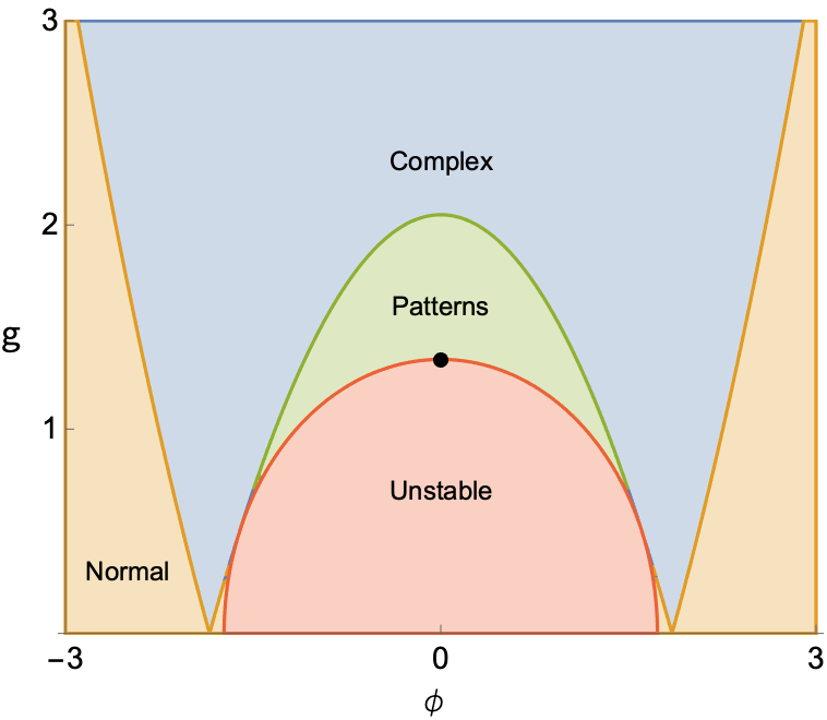
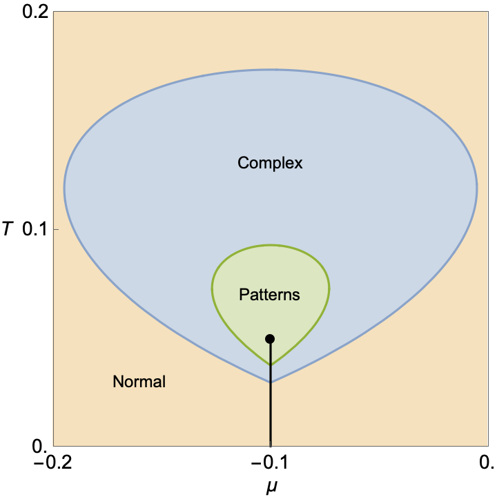
Now, we examine nonzero values, varying and while holding and fixed. We again start by analyzing in the plane. In Fig. 1, as expected we see four phases: stable, unstable, complex, and patterned. A spinodal line separates the unstable and patterned regions. A second-order critical point lies on the spinodal line at .
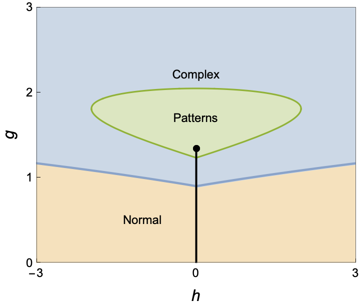
We can Legendre-transform these results into the plane. As in the normal model, metastable states in the complex (blue) phase and unstable states (red) disappear and collapse into a critical line running up the axis. This line is a first-order phase transition terminating in a second-order critical endpoint; i.e., exhibits a discontinuity as we vary past . Note that after the Legendre transform, the critical endpoint has relocated from the edge of the patterned region to its interior.
3.2 Simulations
Medina and Ogilvie have developed a technique to recast -QFTs into a fully real form [9]: all we need to do is take a Fourier transform of appropriate fields within the path integral. To simulate in eq. (6), we make such a transform with respect to the field (not the position-space variable ). The dual action is real, positive, and thus simulatable:
| (9) |
In Fig. 2, we display a small sample of lattice simulation results. We notice that the region of pattern formation in lattice simulations using as a parameter agrees well with the region we determined using tree-level analytics using as a parameter in Fig. 1.
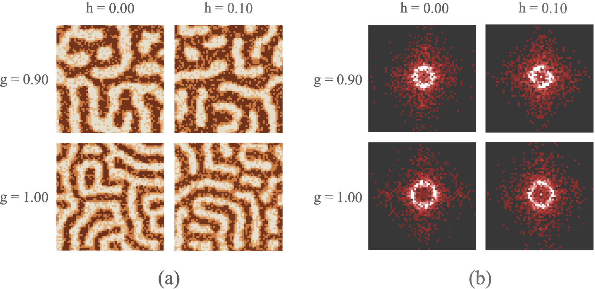
The nature of the patterned field configurations strongly suggests that the patterned region comprises a single thermodynamic phase. As we vary the parameters , the pattern morphologies evolve smoothly. When we take a Fourier transform of a configuration from to , we see that patterned configurations in -space become ring-shaped in -space. The only evidence for a sharp thermodynamic phase transition in the patterned region is at for low values of , which is where we have analytically determined the critical line and critical endpoint to be located. Along this line, jumps in a first-order transition that terminates at a second-order point.
4 Phase structure of a QCD-like model
Let us now apply these methods to a simple effective model of finite-density QCD, a heavy quark theory [2]. Consider the action
| (10) |
The first term is a mean-field heavy quark determinant; we parametrize the Polyakov loop as and absorb parameters into a coefficient . The second term characterizes Polyakov loop interactions with a potential split into attractive and repulsive pieces .
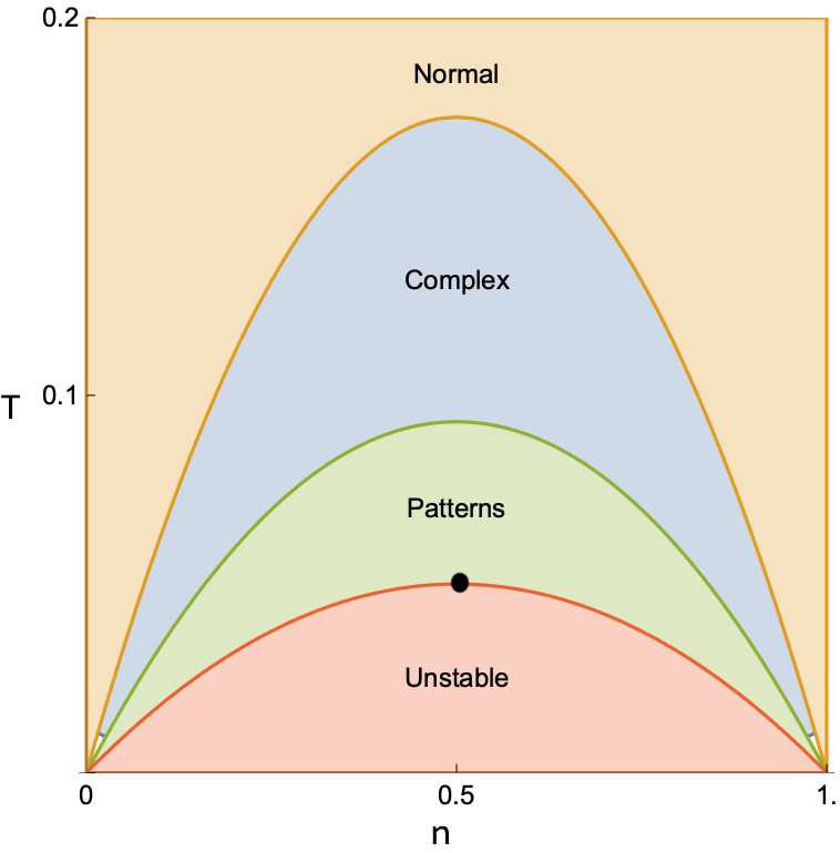
We can determine the phase diagram of eq. (10) straightforwardly using the procedure outlined in Sec. 3. It is instructive to first examine a simple choice of potentials: Yukawa interactions with . We plot the phase diagram of the Yukawa model in both the fermion density vs. plane, as well as in the chemical potential vs. plane in Fig. 3.
The phase diagram structure looks remarkably similar to that of eq. (6): around the critical endpoint, we find a patterned region, surrounded by a sinusoidally-modulated region, which is in turn bounded by a disorder line. These behaviors are indeed universal in pattern formation, which raises the possibility that we might see similar phenomena around the critical endpoint of finite-density QCD. The inhomogeneous phase would consist of patterns of deconfined phase within a sea of confined phase, and vice versa.
We can calculate the phase diagram for the full model as in Table 1, and extend the results to the continuum. We write the criterion for stability against pattern formation as
| (11) |
where is the quark number susceptibility and is the quark-quark potential. Note that all terms in this stability criterion are in principle computable on the lattice.
5 Outlook
We believe that the -symmetric framework holds great promise in understanding critical behavior in field theories with sign problems, including finite-density QCD. There are two natural directions in which to proceed. First, we can directly use the techniques shown in these proceedings to tackle more complicated models that incorporate more features of finite-density QCD. For example, dropping the mean-field approximation implicit in eq. (10) allows for a more precise determination of the critical point of a heavy quark model. Also, we can examine the effect of adding in canonical features of QCD like triality and chirality, and see their effect on phase structure. Second, it is important to extend our suite of -inspired analytic and algorithmic techniques to accommodate a wider span of field theories. We are pursuing both lines of research.
References
- [1] P.N. Meisinger and M.C. Ogilvie, PT symmetry in classical and quantum statistical mechanics, Phil. Trans. Roy. Soc. Lond. A 371 (2013) 20120058 [1208.5077].
- [2] M.A. Schindler, S.T. Schindler and M.C. Ogilvie, symmetry, pattern formation, and finite-density QCD, [2106.07092].
- [3] C.M. Bender and S. Boettcher, Real spectra in non-Hermitian Hamiltonians having PT symmetry, Phys. Rev. Lett. 80 (1998) 5243 [physics/9712001].
- [4] M.-A. Miri and A. Alu, Exceptional points in optics and photonics, Science 363 (2019) eaar7709.
- [5] L. Feng, R. El-Ganainy and L. Ge, Non-Hermitian photonics based on parity-time symmetry, Nature Photonics 11 (2017) 752.
- [6] R. El-Ganainy, K.G. Makris, M. Khajavikhan, Z.H. Musslimani, S. Rotter and D.N. Christodoulides, Non-Hermitian physics and PT symmetry, Nature Physics 14 (2018) 11.
- [7] S. Ozdemir, S. Rotter, F. Nori and L. Yang, Parity-time symmetry and exceptional points in photonics, Nature Materials 18 (2019) 783.
- [8] C.M. Bender, P.E. Dorey, C. Dunning, A. Fring, D.W. Hook, H.F. Jones et al., PT Symmetry: in Quantum and Classical Physics, World Scientific (2019), 10.1142/q0178.
- [9] M.C. Ogilvie and L. Medina, Simulation of scalar field theories with complex actions, PoS LATTICE2018 (2018) 157 [1811.11112].
- [10] M.A. Schindler, S.T. Schindler, L. Medina and M.C. Ogilvie, Universality of pattern formation, Phys. Rev. D 102 (2020) 114510 [1906.07288].
- [11] K. Fukushima and T. Hatsuda, The phase diagram of dense QCD, Rept. Prog. Phys. 74 (2011) 014001 [1005.4814].
- [12] M.G. Alford, A. Schmitt, K. Rajagopal and T. Schäfer, Color superconductivity in dense quark matter, Rev. Mod. Phys. 80 (2008) 1455 [0709.4635].
- [13] T. Kojo, Y. Hidaka, L. McLerran and R.D. Pisarski, Quarkyonic Chiral Spirals, Nucl. Phys. A 843 (2010) 37 [0912.3800].
- [14] A. Patel, Flux Tube Model Signals for Baryon Correlations in Heavy Ion Collisions, Phys. Rev. D 85 (2012) 114019 [1111.0177].
- [15] A. Patel, Baryon Number Correlations in Heavy Ion Collisions, PoS LATTICE2012 (2012) 096 [1210.5907].
- [16] H. Nishimura, M.C. Ogilvie and K. Pangeni, Complex saddle points in QCD at finite temperature and density, Phys. Rev. D 90 (2014) 045039 [1401.7982].
- [17] H. Nishimura, M.C. Ogilvie and K. Pangeni, Complex Saddle Points and Disorder Lines in QCD at finite temperature and density, Phys. Rev. D 91 (2015) 054004 [1411.4959].
- [18] H. Nishimura, M.C. Ogilvie and K. Pangeni, Liquid-Gas Phase Transitions and Symmetry in Quantum Field Theories, Phys. Rev. D 95 (2017) 076003 [1612.09575].
- [19] H. Nishimura, M.C. Ogilvie and K. Pangeni, Complex spectrum of finite-density lattice QCD with static quarks at strong coupling, Phys. Rev. D 93 (2016) 094501 [1512.09131].
- [20] O. Akerlund, P. de Forcrand and T. Rindlisbacher, Oscillating propagators in heavy-dense QCD, JHEP 10 (2016) 055 [1602.02925].
- [21] C.M. Bender, Making sense of non-Hermitian Hamiltonians, Rept. Prog. Phys. 70 (2007) 947 [hep-th/0703096].
- [22] S. Weigert, Completeness and orthonormality in PT-symmetric quantum systems, Phys. Rev. A 68 (2003) 062111 [quant-ph/0306040].
- [23] C.M. Bender, S. Boettcher and V.M. Savage, Conjecture on the interlacing of zeros in complex Sturm-Liouville problems, J. Math. Phys. 41 (2000) 6381 [math-ph/0005012].
- [24] S.T. Schindler and C.M. Bender, Winding in non-Hermitian systems, J. Phys. A 51 (2018) 055201 [1704.02028].
- [25] A. Fring and T. Taira, Non-Hermitian gauge field theories and BPS limits, [2103.13519].
- [26] P.D. Mannheim, Extension of the Goldstone and the Englert-Brout-Higgs mechanisms to non-Hermitian theories, 9, 2021 [2109.08714].