Detectability and global observer design for 2D Navier-Stokes equations with uncertain inputs

Abstract

We present simulation friendly detectability conditions for 2D Navier-Stokes Equation (NSE) with periodic boundary conditions, and describe a generic class of “detectable” observation operators: it includes pointwise evaluation of NSE’s solution at interpolation nodes, and spatial average measurements. For “detectable” observation operators we design a global infinite-dimensional observer for NSE with uncertain possibly destabilizing inputs: in our numerical experiments we illustrate $H^{1}$-sensitivity of NSE to small perturbations of initial conditions, yet the observer converges for known and uncertain inputs.

, ,

1 Introduction

Navier-Stokes Equation (NSE)

$$\frac{d\vec{u}}{dt}+(\vec{u}\cdot\nabla)\vec{u}-\nu\Delta\vec{u}+\nabla p=\vec{f}$$ (1.1)

is a basic mathematical model of fluid dynamics: it describes evolution of fluid’s velocity vector-field $\vec{u}$ and scalar pressure field $p$ as a function of initial and boundary conditions, input $\vec{f}$ and coefficient $\nu>0$. NSE has applications in biology, weather prediction, energy forecasting to name a few. It also serves as a mathematical model of turbulence: yet an open problem in 3D, in 2D NSE is used to study turbulence and, in particular, to reveal its connection to deterministic chaos [6]. Indeed, for certain $\nu$ and $\vec{f}$ NSE (1.1) has the unique attractor, which is globally exponentially stable, e.g. $\vec{u}=0$ for $\vec{f}=0$ and any $\nu>0$. However, for small enough $\nu>0$ and a destabilising input $\vec{f}$, NSE’s attractor could be a multidimensional manifold (e.g. [6, 14]), moreover, the attractor could also be chaotic, i.e. initially close-by trajectories might diverge over time on the attractor. For such destabilising inputs classical control problems, e.g. observer design, become challenging, as was noted in [20], especially when attractor’s structure depends on an uncertain input $\vec{f}$.

In this work we generalise the classical notion of detectability for LTI evolution equations [3] to periodic 2D NSE, and introduce detectability conditions: we describe a generic class of “detectable” observation (output) operators $\mathcal{C}$ verifying the proposed conditions (our 1st contribution). Intuitively, “detectable” output $\mathcal{C}\vec{u}$ of (1.1) must provide information about a finite-dimensional subspace where the nonlinear advection term $(\vec{u}\cdot\nabla)\vec{u}$ is not dominated by the diffusion term $-\nu\Delta\vec{u}$ (see also the mechanism of energy cascades [6]). Given such output $\mathcal{C}\vec{u}(t)$ one can then reconstruct the entire state $\vec{u}(t)$ by designing a minimax filter which injects $\mathcal{C}\vec{u}$ so that the reconstruction error in the “unmeasured” infinite-dimensional orthogonal complement of the range of $\mathcal{C}$ will decay thanks to the stabilizing effect of $-\nu\Delta\vec{u}$ akin to the case of detectable LTI systems. More specifically, by employing the direct Lyapunov method, we design an approximate minimax filter for NSE (1.1): we show that $\vec{u}(t)$, the solution of (1.1) for an unknown initial condition $\vec{u}(0)=\vec{u}_{0}$, and for $\vec{f}=\vec{g}+\vec{d}$, $\vec{g}$ – a destabilising known input, $\vec{d}$ – an uncertain bounded input, belongs to $H^{1}$-ellipsoid, centered at the state $\vec{z}(t)$ of Luenberger observer, and its radius decays to $0$ as $t\to\infty$ independently of $\vec{u}_{0}$, provided the uncertain input $\vec{d}$ “perturbs” $\vec{g}$ less frequently in time or $L^{2}(\Omega)$-norm of the perturbation $\vec{d}$ (in space) decays as $t\to\infty$, a remarkable result for turbulent systems which are highly sensitive to small perturbations (our 2nd contribution).
Infinite-dimensional observers for NSEs, employing backstepping as a design technique, were proposed in [20] for Poisseuille flows, a benchmark for turbulence estimation, and in [11] for local observer-based stabilization of NSEs. Disturbance estimation by means of backstepping for linear 1D heat equation was proposed in [5].

The proposed class of “detectable” output operators $\mathcal{C}$ generalizes the notions of so-called determining modes, e.g. spatial averages $\int_{\Omega_{j}}\vec{u}d\vec{x}$ of the solution $\vec{u}$ over squares $\Omega_{j}$ covering the domain $\Omega$ (see e.g. [8, 9, 15]), and determining nodes, e.g. pointwise evaluation $\vec{u}(\vec{x}_{j})$ at finitely many interpolation nodes $\vec{x}_{j}$ (see e.g. [2]), which are well-known in NSE’s literature [6, p.123,p.131]. Our class contains those cases, and more generally it consists of all closed linear operators $\mathcal{C}$ verifying certain inequalities: e.g., spatial averages output $\mathcal{C}\vec{u}=\sum_{j=1}^{N}\int_{\Omega_{j}}\vec{u}d\vec{x}\xi_{j}$, $\xi_{j}$ – normalised indicator of $h\times h$-square $\Omega_{j}$, is detectable if $h^{2}$, the area of $\Omega_{j}$ is small enough for $\vec{u}-\mathcal{C}\vec{u}$ to be “controlled” by $h\nabla\vec{u}$ (Poincaré inequality). These inequalities do not cover boundary-type observations though (see [22, 21]).
We stress that spatial averages outputs are important in real-world applications: for example, short-term solar energy forecasting from a sequence of Cloud Optical Depth (COD) images relies upon estimating averaged velocities of clouds from COD images and uses those as measurements in periodic 2D NSE for cloud velocity prediction [1]; similarly 2D NSE with averaged velocity measurements obtained from Sea Surface Temperature (SST) satellite images were used in [12] to predict short-term SST dynamics.

In this work we build upon preliminary results presented in our conference papers [23, 16]: key differences include detectability conditions and more general case of uncertain inputs. Qualitatively similar results were obtained in [2] where sufficient conditions for convergence of Luenberger observer were proposed for periodic boundary conditions and known inputs. The authors make use of Brezis inequality to bound the nonlinear advection term in the error equation, and derive conditions for observer’s gain and output (e.g. number and size of squares $\Omega_{j}$ for the case of spatial averages outputs), sufficient for convergence. An experimental assesment of these conditions was recently provided in [7]. In contrast, our convergence analysis relies upon a novel one-parametric inequality relating $L^{\infty}$ and $H^{2}$-norms of periodic vector-functions, which for certain values of the parameter reduces to Agmon and Brezis inequalities, and S-procedure widely used in Lyapunov stability analysis. As a result, we get simulation friendly and less conservative detectability conditions: e.g. for the case of spatial averages outputs our estimate of $h^{2}$, the area of squares $\Omega_{j}$, is at least one order of magnitude better for small $\nu>0$, which is of high interest in the case of turbulent flows, and hence for convergence, observer requires averaging the velocity $\vec{u}$ over larger $\Omega_{j}$ (see Remark 3.5 below) so less of squares (“sensors”) is needed, and more importantly, the averaging over larger $\Omega_{j}$ helps reducing the noise hence improving convergence in practice.

1.1 Mathematical preliminaries

Notation.  Let $\mathbb{R}^{n}$ denote Euclidian space of dimension $n$ with inner product $\vec{u}\cdot\vec{v}=\sum_{i=1}^{n}u_{i}v_{i}$, $\mathbb{R}^{n}_{+}$ – non-negative orthant of $\mathbb{R}^{n}$, $\mathbb{R}^{1}_{+}=\mathbb{R}_{+}$, and for $\vec{k},\vec{\ell}\in\mathbb{R}^{n}$ set $\frac{\vec{k}}{\vec{\ell}}=(\frac{k_{1}}{\ell_{1}}\dots\frac{k_{n}}{\ell_{n}})^{\top}$. Let $\mathscr{L}(H)$ denote the space of all closed linear operators $\mathcal{C}$ acting in a Hilbert space $H$ with domain $\mathscr{D}(\mathcal{C})\subset H$. The following functional spaces are standard in NSE’s theory ( [6, p.45-p.48]):

• $L_{p}^{2}(\Omega)$ – space of $\Omega$-periodic functions $u:\Omega\subset\mathbb{R}^{2}\to\mathbb{R}$ with period $\Omega=(-\frac{\ell_{1}}{2},\frac{\ell_{1}}{2})\times(-\frac{\ell_{2}}{2},\frac{\ell_{2}}{2})$ for some $\ell_{1,2}>0$ and inner product $(w,v)=\int_{\Omega}wvdx_{1}dx_{2}$

• $L_{p}^{2}(\Omega)^{2}$ – space of $\Omega$-periodic vector-functions $\vec{u}=\bigl{[}\begin{smallmatrix}u_{1}u_{2}\end{smallmatrix}\bigr{]}$ with inner product $(\vec{u},\vec{\phi})=(u_{1},\phi_{1})+(u_{2},\phi_{2})$ and norm $\|\vec{u}\|^{2}_{L^{2}}=\|u_{1}\|^{2}_{L^{2}}+\|u_{1}\|^{2}_{L^{2}}$

• $H_{p}^{1}(\Omega)=\{u\in L_{p}^{2}(\Omega):\|\nabla u\|_{\mathbb{R}^{2}}\in L_{p}^{2}(\Omega)\}$,
  $H_{p}^{1}(\Omega)^{2}=\{\vec{u}=\bigl{[}\begin{smallmatrix}u_{1}u_{2}\end{smallmatrix}\bigr{]}\in L_{p}^{2}(\Omega)^{2}:u_{1,2}\in H_{p}^{1}(\Omega)\}$ with norm $\|\vec{u}\|^{2}_{H^{1}}=\|\vec{u}\|_{L^{2}}^{2}+\|\nabla\vec{u}\|^{2}_{L^{2}}$ where $\|\nabla\vec{u}\|^{2}_{L^{2}}=\int_{\Omega}\|\nabla\vec{u}\|_{\mathbb{R}^{2}}^{2}dx_{1}dx_{2}$, and $\|\nabla\vec{u}\|_{\mathbb{R}^{2}}^{2}=\|\nabla u_{1}\|_{\mathbb{R}^{2}}^{2}+\|\nabla u_{2}\|_{\mathbb{R}^{2}}^{2}$

• $\mathcal{H}=\{\vec{v}\in[L_{p}^{2}(\Omega)]^{2}:\,\nabla\cdot\vec{v}=0\}$ – space of divergence-free vector-functions $\vec{v}$, $\mathring{\mathcal{H}}=\{\vec{v}\in\mathcal{H}:\quad\int_{\Omega}\vec{v}dxdy=0\}$ – subspace of $\mathcal{H}$ of $\vec{v}$ with zero mean components

• $\mathcal{V}=\{\vec{v}\in[H_{p}^{1}(\Omega)]^{2}:\quad\nabla\cdot\vec{v}=0\}$ and $\mathring{\mathcal{V}}=\{\vec{v}\in\mathcal{V}:\quad\int_{\Omega}\vec{v}dxdy=0\}$

• $L^{2}(0,T,H)$ – space of $H$-valued functions $t\mapsto u(t)\in H$ with finite norm $\|u\|^{2}_{L^{2}(0,T,H)}=\int_{0}^{T}\|u(t)\|_{H}^{2}dt$ for $T\in(0,+\infty)$, e.g. $L^{2}(0,T,\mathring{\mathcal{H}})$ – space of $\vec{v}(t,x_{1},x_{2})$ such that $\int_{0}^{T}\int_{\Omega}\|\vec{v}(t,x_{1},x_{2})\|_{\mathbb{R}^{2}}^{2}dx_{1}dx_{2}<+\infty$ and $\vec{v}(t,\cdot)$ has zero divergence and zero mean for almost all $t\in(0,T)$

• $L^{\infty}(0,T,H)$ – space of $H$-valued functions $t\mapsto u(t)\in H$ such that $\|u(t)\|_{H}\leq C<+\infty$ for some $C>0$ and almost all $t\in(0,T)$, $T\in(0,+\infty)$ with finite norm $\|u\|^{2}_{L^{\infty}}=\|u\|^{2}_{L^{\infty}(0,T,H)}=\min_{C}\{C>0:\|u(t)\|_{H}\leq C\}$

1.1.1 Bounds for $L^{\infty}$-norms of periodic vector-functions

The following lemma is a key building block used below to define detectability and design observer for NSE.

Lemma 1.1.

If $\vec{u}\in H_{p}^{2}(\Omega)^{2}$ and $\int_{\Omega}\vec{u}dx_{1}dx_{2}=0$ then for any $\gamma>0$ it holds:

$$\begin{split}\|\vec{u}\|_{L^{\infty}}&\leq\frac{\log^{\frac{1}{2}}\bigl{(}1+\frac{4\pi^{2}\gamma^{2}}{\ell_{1}\ell_{2}}\bigr{)}\|\vec{u}\|_{H^{1}}}{\sqrt{2\pi}}+\frac{\|\vec{\ell}\|_{\mathbb{R}^{2}}\|\Delta\vec{u}\|_{L^{2}}}{\gamma\sqrt{32\pi^{3}}}\end{split}$$ (1.2)

For $\gamma=\|\vec{u}\|_{H^{1}}^{-\frac{1}{2}}\|\Delta\vec{u}\|_{L^{2}}^{\frac{1}{2}}$ (1.2) gives 2D Agmon inequality [6, p.100]:

$$\begin{split}\|\vec{u}\|_{L^{\infty}}&\leq(\sqrt{\frac{2\pi}{\ell_{1}\ell_{2}}}+\frac{\|\vec{\ell}\|_{\mathbb{R}^{2}}}{\sqrt{32\pi^{3}}})\|\vec{u}\|_{H^{1}}^{\frac{1}{2}}\|\Delta\vec{u}\|_{L^{2}}^{\frac{1}{2}}\end{split}$$ (1.3)

For $\gamma=\|\vec{u}\|_{H^{1}}^{-1}\|\Delta\vec{u}\|_{L^{2}}$ (1.2) gives 2D Brezis inequality [4]:

$$\|\vec{u}\|_{L^{\infty}}\leq\bigl{(}\frac{\|\vec{\ell}\|_{\mathbb{R}^{2}}}{\sqrt{32\pi^{3}}}+\frac{\log^{\frac{1}{2}}(1+\frac{4\pi^{2}\|\Delta\vec{u}\|_{L^{2}}^{2}}{\ell_{1}\ell_{2}\|\vec{u}\|_{H^{1}}^{2}})}{\sqrt{2\pi}}\bigr{)}\|\vec{u}\|_{H^{1}}$$ (1.4)

The proof is given in the appendix.

1.1.2 Navier-Stokes equation: weak formulation and well-posedness in 2D

The classical NSE in 2D is a system of two PDEs defining dynamics of the scalar pressure field $p(x,y)$ and the viscous fluid velocity vector-field $\vec{u}(t,x,y)=[\begin{smallmatrix}u_{1}(t,x,y),u_{2}(t,x,y)\end{smallmatrix}]$ which depends on the initial condition $\vec{u}(0)=\vec{u}_{0}\in\mathcal{H}$, input (e.g. forcing) $\vec{f}=[f_{1},f_{2}]$ and Boundary Conditions (BC), e.g. periodic BC $u_{1,2}(t,x+\ell_{1},y)=u_{1,2}(t,x,y)$, $u_{1,2}(t,x,y+\ell_{2})=u_{1,2}(t,x,y)$. In the vector form it reads as follows:

$$\begin{split}\displaystyle\frac{d\vec{u}}{dt}&+(\vec{u}\cdot\nabla)\vec{u}-\nu\Delta\vec{u}+\nabla p=\vec{f},\quad\nabla\cdot\vec{u}=0\end{split}$$ (1.5)

To eliminate pressure $p$ and obtain an evolution equation just for $\vec{u}$ it is common to use Leray projection [6, p.38]: every vector-field $\vec{u}$ in $\mathbb{R}^{2}$ admits Helmholtz-Leray decomposition, $\vec{u}=\nabla p+\vec{v}$ with $\nabla\cdot\vec{v}=0$ which in turn defines Leray projector, $P_{l}(\vec{u})=\vec{v}$ – an orthogonal projector onto $\mathring{\mathcal{H}}$ (e.g. [6, p.36]). Multiplying (1.5) by a test function $\vec{\phi}\in\mathring{\mathcal{V}}$ (the projection step), and integrating by parts in $\Omega$ allows one to obtain Leray’s weak formulation of NSE in 2D:

$$\frac{d}{dt}(\vec{u},\vec{\phi})+b(\vec{u},\vec{u},\vec{\phi})+\nu((\vec{u},\vec{\phi}))=(\vec{f},\vec{\phi}),\quad\forall\vec{\phi}\in\mathring{\mathcal{V}}$$ (1.6)

with initial condition $(\vec{u}(0),\vec{\phi})=(\vec{u}_{0},\vec{\phi})$. Here

$$b(\vec{u},\vec{w},\vec{\phi}) =(\vec{u}\cdot\nabla w_{1},\phi_{1})+(\vec{u}\cdot\nabla w_{2},\phi_{2}),$$

$$((\vec{u},\vec{\phi})) =(\nabla u_{1},\nabla\phi_{1})+(\nabla u_{2},\nabla\phi_{2})$$

In what follows we will be using some properties of the trilinear form $b$ and Stokes operator $\vec{u}\mapsto A\vec{u}=-P_{l}\Delta\vec{u}$, a self-adjoint positive operator with compact inverse, which coincides with $\Delta\vec{u}$ for periodic BC (see [6, p.52]): for $\vec{u}\in\mathscr{D}(A)$ and $\vec{\phi}\in\mathring{\mathcal{V}}$

$$(A\vec{u},\vec{\phi}) =((\vec{u},\vec{\phi})),\,(A\vec{u},\vec{u})=((\vec{u},\vec{u}))\geq\lambda_{1}(\vec{u},\vec{u})$$ (1.7)

$$(A\vec{u},A\vec{u}) =(A(A^{\frac{1}{2}})\vec{u},(A^{\frac{1}{2}})\vec{u})\geq\lambda_{1}(A\vec{u},\vec{u})$$ (1.8)

$$\lambda_{1} =4\pi^{2}/\max\{\ell_{1},\ell_{2}\}^{2}$$ (1.9)

$$b(\vec{u},\vec{v},\vec{\phi}) =-b(\vec{u},\vec{\phi},\vec{v})$$ (1.10)

$$b(\vec{u},\vec{v},\vec{v}) =0,\quad b(\vec{v},\vec{v},A\vec{v})=0$$ (1.11)

Next Lemma collects results from [6, p.58, Th.7.4, p.99, f.(A.42), p.102, f.(A.66)-(A.67)] on existence, uniqueness, regularity and input-to-state stability of NSE’s weak (strong) solution $\vec{u}$, and bounds for $A\vec{u}$. Classical smoothness of $\vec{u}$ requires further constraining of $\vec{f}$, $\vec{u}_{0}$ [6, p.59].

Lemma 1.2.

Let $\vec{u}_{0}\in\mathring{\mathcal{H}}$ and $\vec{f}\in L^{2}(0,\bar{T},\mathring{\mathcal{H}})$. Then, on $[0,\bar{T}]$ there exist the unique weak solution $\vec{u}\in C(0,\bar{T},\mathring{\mathcal{H}})$ of NSE (1.6), and the components of $\vec{u}=\begin{smallmatrix}[u_{1}&u_{2}]\end{smallmatrix}$ verify: $u_{i},(u_{i})_{x,y}\in L^{2}(\Omega\times(0,\bar{T}))$. If $\vec{u}_{0}\in\mathring{\mathcal{V}}$ then the weak solution coincides with the strong solution of (1.6), and

$$\frac{du_{i}}{dt},(u_{i})_{x},(u_{i})_{y},(u_{i})_{xy}\in L^{2}(\Omega\times(0,\bar{T}))$$

i.e. $\vec{u}\in C(0,\bar{T},\mathring{\mathcal{V}})\cap L^{2}(0,\bar{T},\mathscr{D}(A))$. If in addition $\vec{f}\in L^{\infty}(\mathbb{R}_{+},\mathring{\mathcal{H}})$ then $(\,\|\vec{f}\|_{L^{\infty}}=\|\vec{f}\|_{L^{\infty}(\mathbb{R}_{+},\mathring{\mathcal{H}})}$ for short$)$:

$$\|\vec{u}(\cdot,t)\|^{2}_{L^{2}}\leq\frac{\|\vec{f}\|^{2}_{L^{\infty}}}{(\nu\lambda_{1})^{2}}+e^{(-\lambda_{1}\nu)(t-s)}\|\vec{u}(\cdot,s)\|^{2}_{L^{2}}$$ (1.12)

$$\|\nabla\vec{u}(\cdot,t)\|^{2}_{L^{2}}\leq\frac{\|\vec{f}\|^{2}_{L^{\infty}}}{\nu^{2}\lambda_{1}}+e^{(-\lambda_{1}\nu)(t-s)}\|\nabla\vec{u}(\cdot,s)\|^{2}_{L^{2}}$$ (1.13)

$$\frac{1}{\bar{T}}\int_{t}^{\bar{T}+t}\|A\vec{u}\|^{2}_{L^{2}}ds\leq\theta_{t,\bar{T}}:=\frac{2\|\vec{f}\|^{2}_{L^{\infty}}}{\bar{T}\nu^{3}\lambda_{1}}+$$ (1.14)

$$\quad+\frac{1}{\bar{T}}\int_{t}^{\bar{T}+t}\frac{\|\vec{f}(s)\|^{2}_{L^{2}}}{\nu^{2}}ds+\frac{2e^{(-\lambda_{1}\nu)t}\|\nabla\vec{u}_{0}\|^{2}_{L^{2}}}{\bar{T}\nu}$$ (1.15)

2 Problem statement

Generalizing the classical definition of detectability for LTI systems [3] we say that NSE is detectable w.r.t. output operator $\mathcal{C}$ if the distance (in space) between any two solutions corresponding to different initial conditions and inputs converges to zero over time, provided so does the distance between their respective outputs and inputs:

Definition 2.1.

For $\vec{f},\vec{F}\in L^{\infty}(\mathbb{R}_{+},\mathring{\mathcal{H}})$ let $\vec{u}$ and $\vec{z}$ solve

$$\displaystyle\frac{d}{dt}(\vec{u},\vec{\phi}) +b(\vec{u},\vec{u},\vec{\phi})+\nu((\vec{u},\vec{\phi}))=(\vec{f},\vec{\phi})\,,\vec{u}(0)\in\mathring{\mathcal{V}}$$ (2.1)

$$\displaystyle\frac{d}{dt}(\vec{z},\vec{\phi}) +b(\vec{z},\vec{z},\vec{\phi})+\nu((\vec{z},\vec{\phi}))=(\vec{F},\vec{\phi})\,,\vec{z}(0)\in\mathring{\mathcal{V}}$$ (2.2)

NSE is called detectable in $\mathring{\mathcal{V}}$ w.r.t. an linear output operator $\mathcal{C}\in\mathscr{L}(\mathcal{H})$ if the following conditions

$$\mathrm{A)}~{}\exists T>0:\limsup_{t\to\infty}\frac{1}{T}\int_{t}^{t+T}\|\mathcal{C}(\vec{u}(\cdot,s)-\vec{z}(\cdot,s))\|_{L^{2}}^{2}ds=0$$

$$\mathrm{B)}~{}\exists T>0:\limsup_{t\to\infty}\frac{1}{T}\int_{t}^{t+T}\|\vec{f}(\cdot,s)-\vec{F}(\cdot,s)\|_{L^{2}}^{2}ds=0$$

imply state convergence in $\mathring{\mathcal{V}}$: $\|\vec{u}(\cdot,t)-\vec{z}(\cdot,t)\|_{\mathring{\mathcal{V}}}\underset{t\to\infty}{\to}0$.

In practice, typical output operators $\mathcal{C}$ are either pointwise evaluations (see Example 2.2 below), or of projection type, i.e. $\mathcal{C}\vec{u}$ is a projection of $\vec{u}$ onto a subspace (see Example 2.1 below). The following definition introduces two classes of output operators $\mathcal{C}$ which generalize projection type and pointwise evaluation type observations:

Definition 2.2.

Take $\mathcal{C}\in\mathscr{L}(L^{2})$ such that $\mathcal{V}\subseteq\mathscr{D}(\mathcal{C})$ and fix $h>0$. $\mathcal{C}$ is said to be of class $\mathscr{C}_{1}(h,\Omega)$ or of class $\mathscr{C}_{2}(h,\Omega)$ if (2.3) or  (2.4) respectively holds for some $C_{\Omega}>0$

$$\forall\vec{u}\in\mathring{\mathcal{V}}:\quad\|\vec{u}-\mathcal{C}\vec{u}\|_{L^{2}}^{2} \leq h^{2}C_{\Omega}\|\nabla\vec{u}\|_{L^{2}}^{2}$$ (2.3)

$$\forall\vec{u}\in\mathscr{D}(A):\quad\|\vec{u}-\mathcal{C}\vec{u}\|_{L^{2}}^{2} \leq h^{2}C_{\Omega}\|\Delta\vec{u}\|_{L^{2}}^{2}$$ (2.4)

Example 2.1.

The class $\mathscr{C}_{1}(h,\Omega)$ generalizes the notion of so-called determining modes for NSE (e.g. [6, p.123]). The case of determining modes corresponds to $\mathcal{C}\in\mathscr{C}_{1}(h,\Omega)$ of finite rank, $\mathcal{C}\vec{u}$ represents the projection of $\vec{u}$ onto a certain finite-dimensional subspace of $\mathcal{H}$, and in this case $\mathcal{C}$ is bounded in $\mathcal{H}$. As an example, consider the case of spatial averages over a partition of $\Omega$ (e.g. [9, 2]): Let $\Omega=\cup_{j=1}^{N}\Omega_{j}$, $\Omega_{j}\cap\Omega_{i}=\varnothing$ for $i\neq j$, $\Omega_{j}$ – a rectangle with sides of length $h_{x}^{j}$ and $h_{y}^{j}$ respectively, and let $\xi_{j}$ denote the indicator function of $\Omega_{j}$. Let

$$\mathcal{C}\vec{u}(x,y)=\sum_{j=1}^{N}\bigl{[}\begin{smallmatrix}(u_{1},\xi_{j})\\ (u_{2},\xi_{j})\end{smallmatrix}\bigr{]}\frac{\xi_{j}(x,y)}{h_{x}^{j}h_{y}^{j}},\quad\xi_{j}(x,y)=1,(x,y)\in\Omega_{j}$$

Then (2.3) holds for $h^{2}=\max_{j}(\max\{h_{x}^{j},h_{y}^{j}\})^{2}$ and $C_{\Omega}=(4\pi^{2})^{-1}$ by Poincaré inequality (1.7).

Example 2.2.

The class $\mathscr{C}_{2}(h,\Omega)$ generalizes notion of so-called determining nodes for NSE (see e.g. [6, p.131]). The case of determining nodes corresponds to $\mathcal{C}\in\mathscr{C}_{2}(h,\Omega)$ of the form $\mathcal{C}\vec{u}=\sum_{j=1}^{n}\vec{u}(t,\vec{x}_{j})\vec{\phi}_{j}$ for some grid nodes $\vec{x}_{j}\in\Omega$ and functions $\vec{\phi}_{j}\in H^{1}_{p}(\Omega)^{2}$. Clearly, $\mathcal{C}$ is not bounded in $\mathcal{H}$ as it is defined for $\vec{u}\in H^{2}_{p}(\Omega)^{2}\cap\mathcal{H}$, but it is a closed linear operator such that $\mathscr{D}(A)\subset\mathscr{D}(C)$. As an example, consider the case of pointwise evaluations over nodes $\vec{x}_{j}$ of a finite element grid, here $\vec{\phi}_{j}$ are 2D hat basis functions. In this case $\mathcal{C}$ verifies (2.4) with constants $h$ and $C_{\Omega}$ which can be found in [13, Th 12.3.4].

With the above two definitions in mind we are ready to state goals of the paper:

• detectability: find sufficient conditions for detectability (as per Definition 2.1) of NSE w.r.t. any output operator $\mathcal{C}\in\mathscr{C}_{1}(h,\Omega)$ or $\mathcal{C}\in\mathscr{C}_{2}(h,\Omega)$

• observer design: given output $\mathcal{C}\vec{u}$ of (2.1) to construct an output feedback control $\vec{F}$ such that conditions $A)$ and $B)$ hold and so, by detectability, $\vec{z}$ converges to $\vec{u}$ in $\mathring{\mathcal{V}}$ independently of $\vec{u}(0)$ and $\nabla\vec{u}(0)$

3 Main results

3.1 Sufficient conditions for detectability

Recall the classes $\mathscr{C}_{1}(h,\Omega)$ and $\mathscr{C}_{2}(h,\Omega)$ of observation operators $\mathcal{C}$ introduced above in Def. 2.2. The following proposition demonstrates existence of a constant $h>0$ for each of $\mathscr{C}_{1}(h,\Omega)$ and $\mathscr{C}_{2}(h,\Omega)$ such that NSE is detectable (as per Definition 2.1). However, as is, this proposition is of rather theoretical value as to compute $h>0$ for numerical simulations one needs to know certain interpolation constants which are either unknown or very concervative. The question of how to use this result for estimating $h$ in numerical simulations will be addressed below.

Proposition 1.

Recall Def. 2.1: let $\vec{z},\vec{u}$ solve (2.1)-(2.2) for $\vec{f},\vec{F}\in L^{\infty}(\mathbb{R}_{+},\mathring{\mathcal{H}})$. Recall from [6, p.100,(A.47)] an interpolation inequality for $\nabla\vec{u}$, and define constants $C_{1,2}$:

$$\forall\vec{u}\in\mathscr{D}(A):\|\nabla\vec{u}\|^{2}_{L^{2}}\leq C_{\nabla}\|\vec{u}\|_{L^{2}}\|A\vec{u}\|_{L^{2}}$$ (3.1)

$$C_{1}^{2}=(1+\lambda_{1}^{-1})/(2\pi),\quad C_{2}^{2}=\|\vec{\ell}\|^{2}_{\mathbb{R}^{2}}/(32\pi^{3})$$ (3.2)

Take $\mathcal{C}\in\mathscr{C}_{1}(h,\Omega)$. Then NSE is detectable in $\mathring{\mathcal{V}}$ if for some $1<\kappa<<2$ and $\Gamma>0$

$$h<\frac{\lambda_{1}^{\frac{1}{2}}\nu\bigl{(}\frac{3\nu}{4}-\frac{C_{2}}{\lambda_{1}\Gamma}\bigr{)}}{C_{1}C_{\nabla}C^{\frac{1}{2}}_{\Omega}\kappa^{\frac{1}{2}}\|\vec{f}\|_{L^{\infty}(\mathbb{R}_{+},\mathring{\mathcal{H}})}\log^{\frac{1}{2}}\bigl{(}1+\frac{4\pi^{2}\kappa\|\vec{f}\|_{L^{2}}^{2}\Gamma^{2}}{\nu^{2}\ell_{1}\ell_{2}}\bigr{)}}$$ (3.3)

moreover, if $\mathcal{C}\in\mathscr{C}_{2}(h,\Omega)$ then NSE is detectable in $\mathring{\mathcal{V}}$ if $h$ verifies (3.3) without $\lambda_{1}^{\frac{1}{2}}$ in the numerator.

The proof is provided in the appendix.

3.2 Observer design

As noted above, condition (3.3) is hard to use in simulations. Below we build on (3.3) and propose “simulation friendly” conditions for $h$ (see $C1,C2$ of Theorem 3.2): it is demonstrated that plugging Luenberger-type output feedback $\vec{F}=\vec{g}+L\mathcal{C}(\vec{u}-\vec{z})$ into (2.2) ensures output and input convergence (conditions $A)$ and $B)$ of Def. 2.1), and as a result implies state convergence in $\mathring{\mathcal{V}}$: $\|\vec{u}(\cdot,t)-\vec{z}(\cdot,t)\|_{\mathring{\mathcal{V}}}\to 0$.

Lemma 3.1 (Wellposedness).

Let $\vec{u}$ solve (2.1). For any $\vec{g}\in L^{\infty}(\mathbb{R}_{+},\mathring{\mathcal{H}})$ there is the unique $\vec{z}\in L^{\infty}(\mathbb{R}_{+},\mathring{\mathcal{V}})\cap L^{2}(t_{0},t_{1},\mathscr{D}(A))$, $0\leq t_{0}<t_{1}<+\infty$ such that

$$\displaystyle\frac{d}{dt}(\vec{z},\vec{\phi})+b(\vec{z},\vec{z},\vec{\phi})+\nu((\vec{z},\vec{\phi}))=(\vec{F},\vec{\phi})\,,\phi\in\mathring{\mathcal{V}}$$ (3.4)

$$\vec{F}=\vec{g}+L\mathcal{C}(\vec{u}-\vec{z})$$ (3.5)

provided $\mathcal{C}\in\mathscr{C}_{1}(h,\Omega)$ and $Lh^{2}C_{\Omega}\leq 2\nu$, or $\mathcal{C}\in\mathscr{C}_{2}(h,\Omega)$ and $LhC_{\Omega}^{\frac{1}{2}}\leq\nu$.

The proof is given in the appendix.

Theorem 3.2.

Assume that (i) $\vec{u}$ solves (2.1) for unknown $\vec{u}(0)\in\mathring{\mathcal{V}}$ and $\vec{f}$, and (ii) $\vec{f}=\vec{g}+\vec{d}$ for a known $\vec{g}\in L^{\infty}(\mathbb{R}_{+},\mathring{\mathcal{H}})$, $C_{\vec{g}}=\|\vec{g}\|_{L^{\infty}(\mathbb{R}_{+},\mathring{\mathcal{H}})}$ and an uncertain input $\vec{d}$ from a ball $\mathscr{E}_{R}=\{\vec{d}:\|\vec{d}\|_{L^{\infty}(\mathbb{R}_{+},\mathring{\mathcal{H}})}\leq R\}$ of radius $R>0$. Let $\vec{z}$ solve (3.4) for $\vec{z}(0)=0$, $L>0$ and $\vec{g}$ as in (ii) above. For $\varepsilon>0$ define $\kappa=1+\varepsilon$ and functions of a parameter $\Gamma$:

$$\hat{L}_{\nabla}(\Gamma) =2(\nu-\frac{\|\vec{\ell}\|_{\mathbb{R}^{2}}}{\sqrt{32\pi^{3}}\lambda_{1}\Gamma})/C_{\Omega},\quad\vec{\ell}=\bigl{[}\begin{smallmatrix}\ell_{1}\\ \ell_{2}\end{smallmatrix}\bigr{]}$$ (3.6)

$$\hat{L}_{\Delta}(\Gamma) =\frac{(\kappa+\kappa\lambda_{1}^{-1})^{\frac{1}{2}}C_{\vec{g}}}{\nu\sqrt{2\pi}}\log^{\frac{1}{2}}\bigl{(}1+\frac{4\pi^{2}\kappa\,C_{\vec{g}}^{2}\,\Gamma^{2}}{\nu^{2}\ell_{1}\ell_{2}}\bigr{)}$$ (3.7)

$$\Theta(\Gamma) =\hat{L}_{\nabla}(\Gamma)/(2\hat{L}_{\Delta}(\Gamma))$$ (3.8)

and let $\Gamma_{\mathrm{max}}>0$ maximize $\Theta(\Gamma)$. Finally assume that

$$\exists T>0:\Sigma_{T}(s)=\sup_{t\geq s}\frac{1}{T}\int_{t}^{t+T}\|\vec{d}(\tau)\|^{2}_{L^{2}}d\tau\xrightarrow{s\to\infty}0$$ (3.9)

and take minimal $t^{\star}>0$ and $T_{1}\geq T$ verifying

$$\begin{split}&\delta(t^{\star})+\frac{2(C_{\vec{g}}+R)^{2}}{C_{\vec{g}}^{2}T_{1}\nu\lambda_{1}}+\frac{2\nu\mathbb{e}^{-\lambda_{1}\nu t^{\star}}\|\nabla\vec{u}_{0}\|^{2}_{L^{2}}}{T_{1}C_{\vec{g}}^{2}}\leq\varepsilon\\ &\delta(t^{\star})=C_{\vec{g}}^{-2}\Sigma_{T_{1}}(t^{\star})+C_{\vec{g}}^{-1}\Sigma_{T_{1}}^{\frac{1}{2}}(t^{\star})\end{split}$$ (3.10)

Then, for $t\geq s\geq t^{\star}$, $V(t)=\|\nabla(\vec{u}(t)-\vec{z}(t))\|^{2}_{L^{2}}$ verifies

$$\begin{split}V(t)&\leq e^{\omega LT_{1}}V(s)e^{(Q(L)-\omega L)(t-s)+\omega LT_{1}\lfloor\frac{t-s}{T_{1}}\rfloor}\\ &+\frac{T_{1}e^{T_{1}(\omega L-Q(L))}}{C_{\Omega}(1-\beta)\hat{L}_{\nabla}(\Gamma_{\mathrm{max}})}\Sigma_{T_{1}}(s)\\ Q(L)&=-L\omega+\hat{L}_{\Delta}(\Gamma_{\mathrm{max}})<0,\end{split}$$ (3.11)

if $\mathcal{C}$, $L$ in (3.4), and $\beta,\omega$ in (3.11) satisfy either $C1$ or $C2$:

• $\mathcal{C}\in\mathscr{C}_{1}(h,\Omega)$ verifies (2.3) with $h^{2}<\beta\Theta(\Gamma_{\mathrm{max}})$ for some $0<\beta<1$, and $L=\beta\hat{L}_{\nabla}(\Gamma_{\mathrm{max}})/h^{2}$, $\omega=1/2$

• $\mathcal{C}\in\mathscr{C}_{2}(h,\Omega)$ verifies (2.4) with $h<\beta C_{\Omega}^{\frac{1}{2}}\theta^{-1}\Theta(\Gamma_{\mathrm{max}})$ for some $0<\beta<1$, $\theta>1$, and $L=\theta\hat{L}_{\Delta}(\Gamma_{\mathrm{max}})$, $\omega=1$

The proof is provided in the appendix.

Remark 3.3.

Condition (3.9) is verified if either (i) the average of $L^{2}$-energy of the uncertain input $\vec{d}$ over time window $(t,t+T)$ decays to $0$, or (ii) the measure of time instants $s$ within a “window” $(t,t+T)$, where $\vec{d}(s,\cdot)$ is “active”, decays to $0$ as the window $(t,t+T)$ slides to infinity ($t\to\infty$). In other words, the case (ii) does not require $\|\vec{d}(s,\cdot)\|_{L^{2}}\to 0$ but requires that the uncertain input $d$ “perturbs” $\vec{g}$ less and less frequently asymptotically.
The rate of decay of $\Sigma_{T}(s)$ to $0$ determines the rate of decay of $V$: indeed, (3.11) implies that

$$\sup_{t>\bar{t}(s)>s}V(t)\leq 2\frac{T_{1}e^{T_{1}(\omega L-Q(L))}}{C_{\Omega}(1-\beta)\hat{L}_{\nabla}(\Gamma_{\mathrm{max}})}\Sigma_{T_{1}}(s)$$

provided $\bar{t}(s)$ is large enough for the impact of the 1st term in r.h.s. of (3.11) be negligible compared to the 2nd term. If $\Sigma_{T}(s)=0$ for $s>s^{\star}$ then $V(t)\to 0$ exponentially after $t=\max\{s^{\star},t^{\star}\}$. In fact, $V\leq V_{1}=\|\vec{u}-\vec{z}\|_{H^{1}(\Omega)}$ and by (1.7) $V_{1}\leq(1+\lambda_{1}^{-1})V$ hence theorem proposes an approximation of minimax filter in the following sence: by (3.11) $\vec{u}(t)$ belongs to $H^{1}$-ellipsoid, centered at $\vec{z}(t)$, and its radius is given by r.h.s. of (3.11).

Remark 3.4.

Parameter $0<\beta<1$ in $C1$ and $C2$ allows to balance “the number of sensors” (e.g. for outputs in the form of spatial averages larger $h^{2}$ means less data as one needs less of $h\times h$-squares to cover $\Omega$), and the impact of $\Sigma_{T}(s)$ onto the decay of $V$: $\beta$ close to $1$ allows to take $h^{2}$ close to its maximal value of $\Theta(\Gamma_{\mathrm{max}})=\max_{\Gamma>0}\Theta(\Gamma)$ at the price of amplifying the impact of the term with $\Sigma_{T}(s)$ in (3.11) proportionally to $1/(1-\beta)$. If $\Sigma_{T}(s)=0$ for $s>s^{\star}$ one can set $\beta=1$. Parameter $\theta>1$ is relevant only for outputs of $\mathscr{C}_{2}(h,\Omega)$-class, it is independent of $\beta$ and allows one to balance convergence speed and amount of observations: larger $\theta$ will imply faster convergence rate at the price of decreasing $h$ proportionally to $1/\theta$. Interestingly, $L$ increases with the decrease of $h$ as per $C1$ but is independent of $h$ if the case $C2$.

Remark 3.5.

Let us compare our upper bound for $h^{2}$ obtained above for $\mathcal{C}\in\mathscr{C}_{1}(h,\Omega)$, namely $h^{2}<\beta\Theta(\Gamma_{\mathrm{max}})$ to the state-of-the-art result of [2, Prop.2]:

$$h^{2}\leq\nu\mathcal{T}(\nu)=C_{\Omega}^{-1}\bigl{(}3\nu\lambda_{1}(2c\log(2)c^{\frac{3}{2}}+8c\log(1+G))G\bigr{)}^{-1},$$ (3.12)

where $G=\frac{\|\vec{f}\|_{L^{\infty}(\mathbb{R}_{+},\mathring{\mathcal{H}})}}{\lambda_{1}\nu^{2}}$ and the constant $c$ comes from Brezis inequality $\|\vec{u}\|_{L^{\infty}}\leq c\|\nabla\vec{u}\|_{L^{2}}(1+\log\frac{\|A\vec{u}\|_{L^{2}}^{2}}{\lambda_{1}\|\nabla\vec{u}\|_{L^{2}}^{2}})^{\frac{1}{2}}$ for $\vec{u}\in\mathscr{D}(A)$ [6, p.100, (A.50)]. Clearly,

$$c=\sup_{\vec{u}\in\mathscr{D}(A):\|\nabla\vec{u}\|_{L^{2}}>0}\|\vec{u}\|_{L^{\infty}}\|\nabla\vec{u}\|^{-1}_{L^{2}}(1+\log\frac{\|A\vec{u}\|_{L^{2}}^{2}}{\lambda_{1}\|\nabla\vec{u}\|_{L^{2}}^{2}})^{-\frac{1}{2}}$$

and so $c\geq c_{1}$ for $c_{1}=\|\vec{u}_{1}\|_{L^{\infty}}\|\nabla\vec{u}_{1}\|^{-1}_{L^{2}}(1+\log\frac{\|A\vec{u}_{1}\|_{L^{2}}^{2}}{\lambda_{1}\|\nabla\vec{u}_{1}\|_{L^{2}}^{2}})^{-\frac{1}{2}}$ and $\vec{u}_{1}\in\mathscr{D}(A)$ with components $u_{1}=-\cos(2\pi x)\sin(2\pi y)$ and $u_{2}=\cos(2\pi y)\sin(2\pi x)$. It is easy to compute that $c_{1}=(2\pi)^{-1}$. Since the r.h.s. of (3.12), $\mathcal{T}(\nu)$ increases if we substitute $c$ with $c_{1}$, and so the upper bound on $h^{2}$ improves, below we compare $\Theta(\Gamma_{\mathrm{max}})$ vs. $\mathcal{T}(\nu)$ with $c=c_{1}=(2\pi)^{-1}$ over the interval $\nu\in[10^{-6},10^{-1}]$. To match the setting of [2] we assume that $\ell_{1,2}=1$, $\|\vec{f}(s)-\vec{g}(s)\|_{\mathbb{R}^{2}}=0$ for $s>s^{\star}$ so we can use $\beta=1$, we also take $\|\vec{f}\|_{L^{\infty}(\mathbb{R}_{+},\mathring{\mathcal{H}})}=C_{\vec{f}}=1$ and $\kappa=2$. We get that $\log_{10}\frac{\Theta(\Gamma_{\mathrm{max}})}{\mathcal{T}(\nu)}=1.33$ for $\nu=10^{-6}$ and $0.58$ for $\nu=10^{-1}$ and LogLog-plot of $\Theta$ and $\mathcal{T}$ over $\nu\in[10^{-6},10^{-1}]$ is given in Fig. 1. Obviously, for small $\nu$ our upper bound is at least one order of magnitude better.

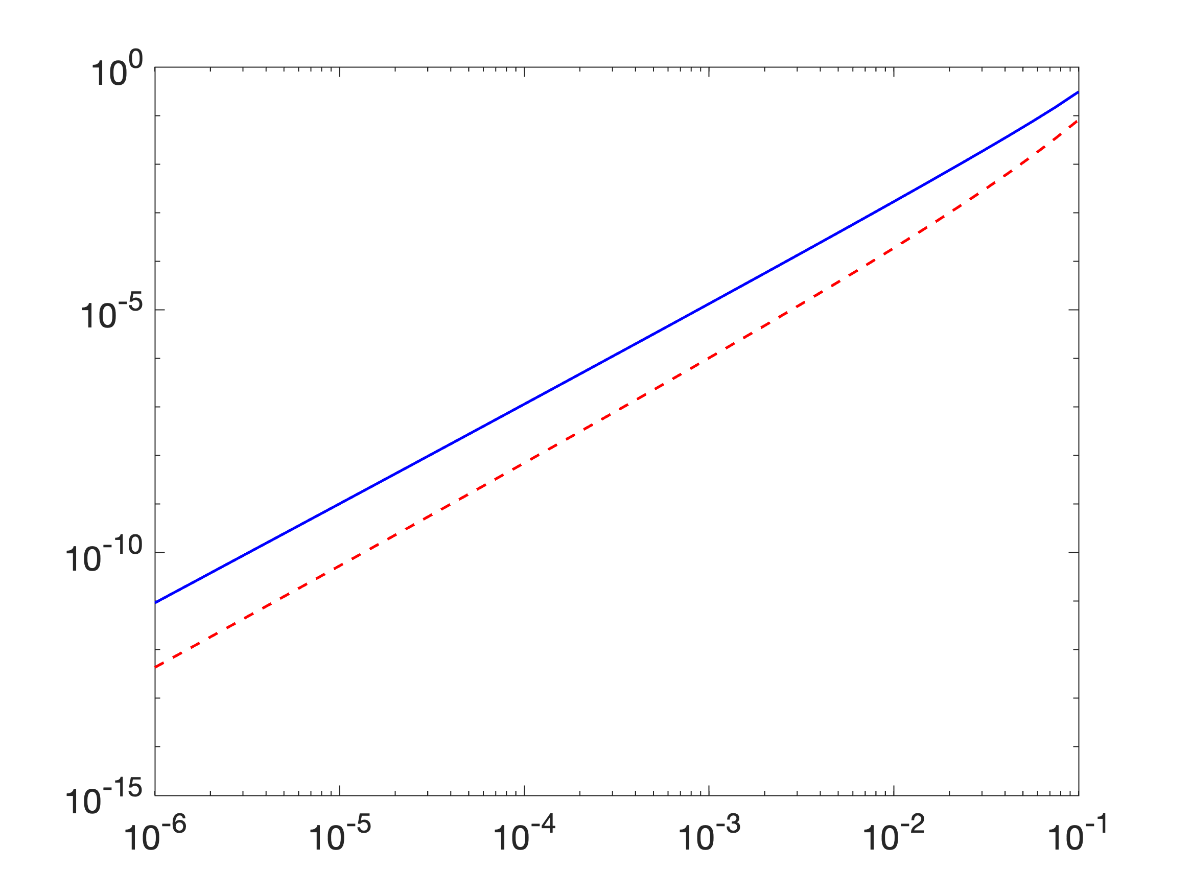
Figure 1: LogLog-plot of upper-bounds for $h^{2}$: $\Theta(\Gamma_{\mathrm{max}})$ (blue) vs. $\mathcal{T}(\nu)$ (red) with $c=c_{1}=(2\pi)^{-1}$ for $\nu\in[10^{-6},10^{-1}]$.

4 Experiments

In what follows we first illustrate sensitivity of NSE with destabilizing Kolmogorov input to small perturbations of initial conditions. Then we illustrate convergence of the observer for the case of known inputs. And finally, we perform a crash-test: we take observations generated by one numerical method, and use them in the observer discretised by a different method.
For the crash-test we generate spatial averages outputs by a numerical solver, referred to as FFT-solver. FFT-solver is a pseudo-spectral numerical method, which relies upon vorticity-streamfunction formulation of NSE. It is exactly divergence free (as required by continuous formulation) and has spectral convergence property in space: its convergence rate in $H^{1}$ automatically increases with the degree of smoothness of initial conditions and inputs. For time discretisation we used 2nd order implicit midpoint with 5 iterations; an open-source implementation of FFT-solver with different time-stepping is available in jax-cfd package. Then, we discretise the observer by a less accurate solver, referred to as FEM-solver. FEM-solver is implemented using Finite Element Method (based on Oasis Python package [17]) with 2nd order triangular elements providing global 1st order convergence rate in space. It also employs 2nd order Backward Differencing scheme for time discretisation. FEM-solver is not divergence free as it relies upon iterative minimization of velocity divergence at every time step. The immense differences between those solvers are pronounced on finite grids used below and their impact on observer, discretized by FEM-solver, is described as an unknown bounded disturbance $\vec{d}$.
Experiment setup. We take a shifted domain $\Omega=[0,\ell_{1}]\times[0,\ell_{2}]$ with $\ell_{1}=\ell_{2}=2\pi$, and a destabilizing input is taken to be $\vec{g}(x,y)=[-5\sin(10y),0]^{\top}$. The initial velocity $\vec{u}(0)$ is generated randomly and taken such that $\|\vec{u}(0)\|_{H^{1}}\approx 9.6$. Both solvers do $1000$ steps forward in time with timestep $\Delta t=0.01$. Spatial resolution varies as detailed below.
Turbulent behaviour. Top panel of Fig. 2 illustrates the sensitivity of NSE to small perturbations of the Initial Condition (IC) measured in $H^{1}$-norm: red curve shows dynamics of $H^{1}$-distance between two trajectories, $\vec{u}$ and $\vec{v}$ obtained by high-precision FFT-solver on $256\times 256$-grid with $\nu=0.01$ and the same input $\vec{g}$; $\vec{u}$ and $\vec{v}$ are close by initially, $\|\vec{u}(0)-\vec{v}(0)\|_{H^{1}}<10^{-4}\|\vec{u}(0)\|_{H^{1}}$. If we repeat the same simulation but for $\nu=0.1$ NSE becomes stable: $H^{1}$-distance between two trajectories decays (blue curve). Bottom panel of Fig. 2 shows dynamics of $H^{1}$-norm of two trajectories with same ICs and input but different $\nu$: for $\nu=0.1$ $H^{1}$-norm levels off, and the flow is laminar (stable) as shown on Fig. 3(a), in contrast, for $\nu=0.01$ $H^{1}$-norm is changing and the flow is turbulent as shown on Fig. 3(b).

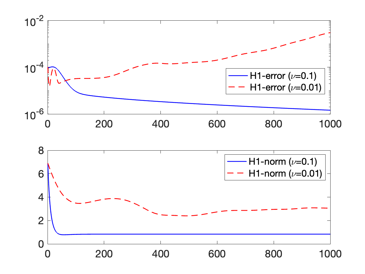
Figure 2: Top panel: $H^{1}$-relative difference of initially close-by trajectories for different $\nu$ over time. Bottom panel: $H^{1}$-norm dynamics of solution with the same initial condition and input for different $\nu$ over time.

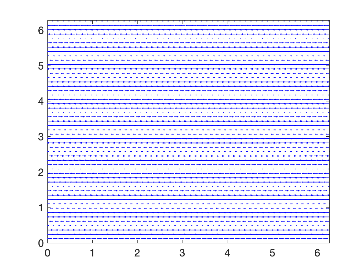
(a) Example of non-turbulent velocity for $\nu=0.1$ (at final time)

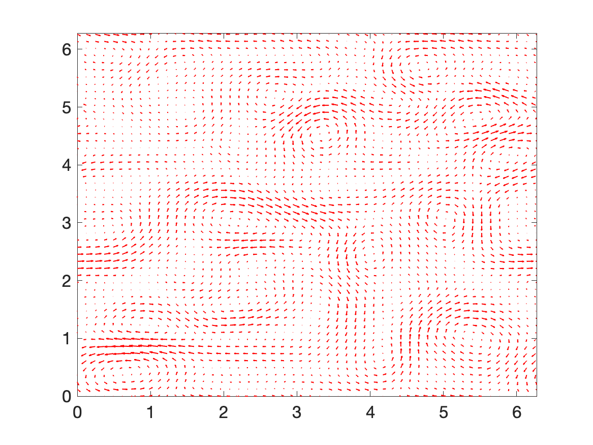
(b) Example of turbulent velocity for $\nu=0.01$ (at final time)

Figure 3: Turbulence: velocity snapshots

Known input. In this test we show that detectability conditions of Theorem 3.2 are indeed simulation friendly: $\mathcal{C}$ is taken to be spatial averages over squares $\Omega_{j}$ covering $\Omega$, and $h^{2}$ in (2.3) is the area of the largest $\Omega_{j}$, thus $h^{2}$ in fact determines the number of squares (sensors) required for convergence. $h^{2}$ is found from $C1$ (Theorem 3.2): since $\vec{d}=0$ it follows that we can set $R=0$, $\beta=1$ (as per Remark 3.4). Also $\Sigma_{T}(s)=0$ for any $T>0$. Hence (3.10) holds for every $T_{1}=T>0$ and $\varepsilon>0$ such that $2/(\nu\lambda_{1})+2\nu e^{-\lambda_{1}\nu t^{\star}}\|\nabla\vec{u}_{0}\|^{2}_{L^{2}}C_{\vec{g}}^{-2}\leq\varepsilon T_{1}$ as $\delta(t^{\star})=0$. We set $\varepsilon=0.001$ and $T_{1}=1.01\varepsilon\times 2/(\nu\lambda_{1})$ so (3.10) holds for $t^{\star}$ such that 2nd term of the last inequality is less than $0.01\times 2/(\nu\lambda_{1})$. We plug $\kappa=1+\varepsilon$ into (3.8) and maximize $\Theta$ by using grid search: we find $\Gamma_{\max}=611$. Hence $h^{2}=0.0029$ as per $C1$, and $L=262$. To get outputs we discretize NSE by FEM-solver with quadratic triangular elements constructed on a uniform grid of $256\times 256$ nodes. Then the outputs are plugged into the observer discretized by the same FEM-solver. The $H^{1}$-estimation error is given in Fig. 4 for 1,10 and 50 pressure corrections, which are used in FEM-solver to minimize the numerical divergence: 50 corrections have smallest divergence (red curve). Clearly, reduction of the numerical divergence implies reduction of $H^{1}$-estimation error.

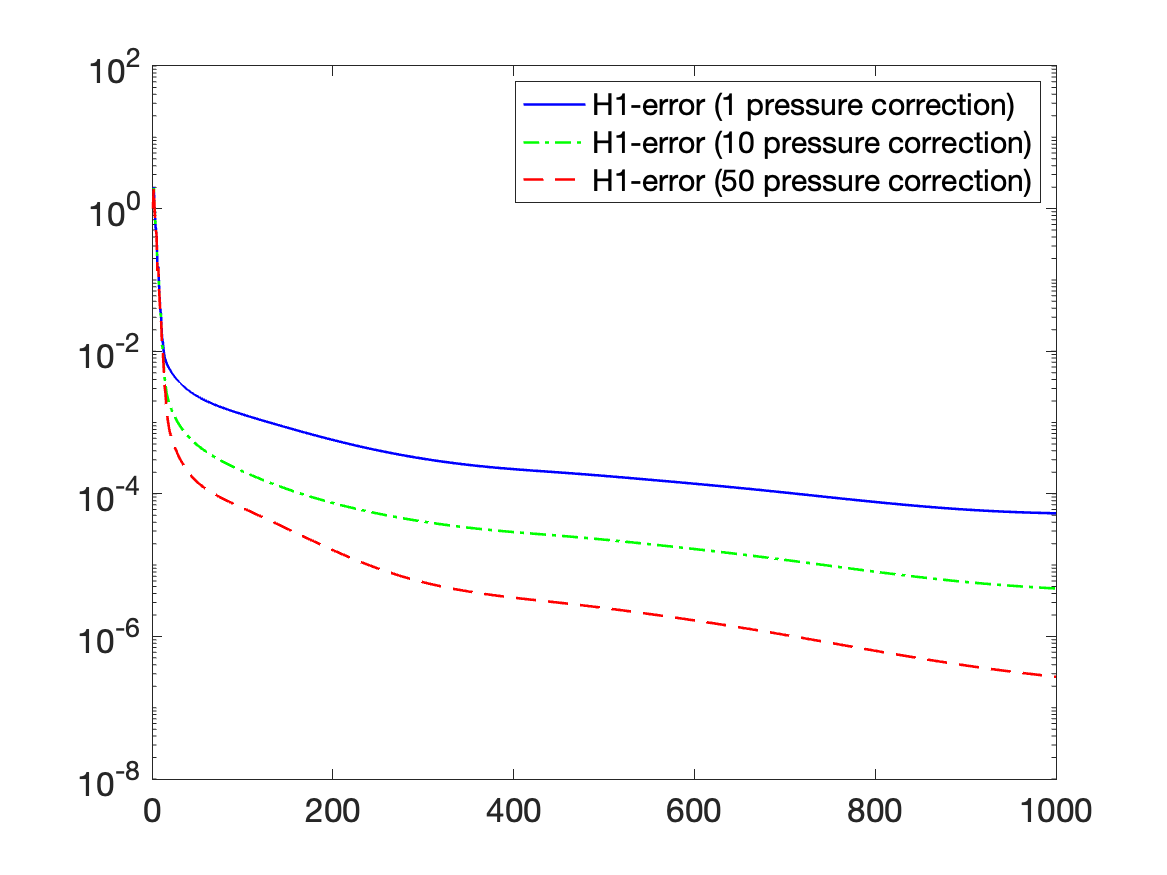
Figure 4: $H^{1}$ rel. est. error (log-scale) over time (1000 timesteps, $\Delta t=0.01$): output and observer generated by FEM-solver.

Uncertain input. In this test we pick $\varepsilon$, $T_{1}$ and $h,L$ as above but use FFT-solver to generate the outputs. The differences between discrete NSEs obtained by FEM-solver and FFT-solver on finite grids are significant, and in fact the former can be seen as the latter but with an additive uncertain input $\vec{d}$ which is expected to get “smaller” for finer grids. And this is exactly what we see on Fig. 5: due to the presence of the disturbance the observer converges into a “zone” which shrinks (in $H^{1}$-norm) when spatial resolution increases from $256\times 256$ to $512\times 512$.

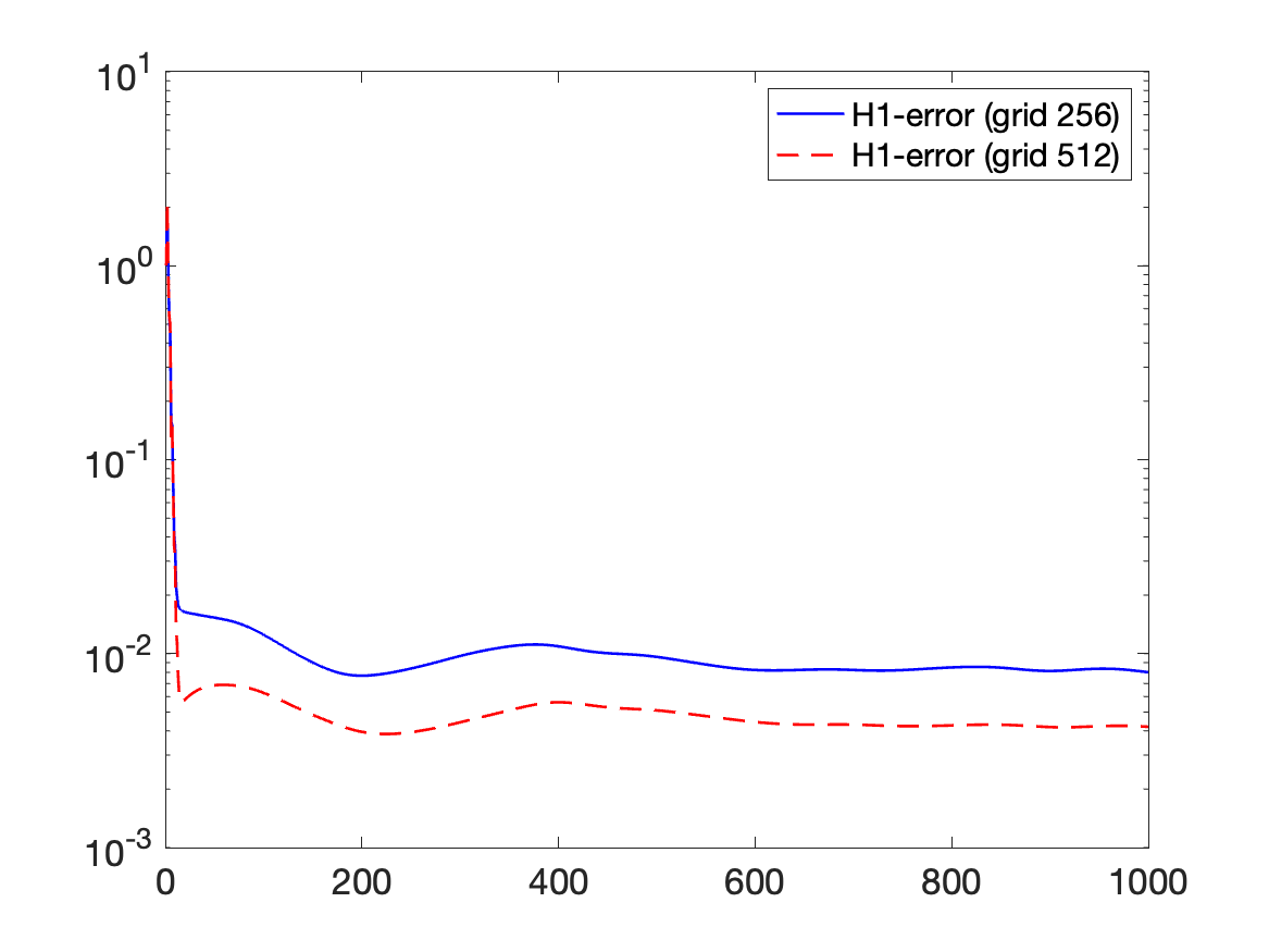
Figure 5: $H^{1}$ rel. est. error (log-scale) over time (1000 timesteps, $\Delta t=0.01$): output generated by FFT-solver, observer – by FEM-solver.

5 Conclusions

We proposed simulation friendly detectability conditions for 2D Navier-Stokes Equation, and designed infinite-dimensional globally converging Luenberger observer for continuous in time measurements. Promising research directions include extending our approach to sampled measurements, and to pointlike measurement where $\Omega_{j}$ do not necessarily cover the entire domain $\Omega$ as studied in [18] for the case of 2D heat equation.

Appendix A Proofs

Proof A.1.

Take $\vec{u}=\bigl{[}\begin{smallmatrix}u&v\end{smallmatrix}\bigr{]}\in[H_{p}^{2}(\Omega)]^{2}$. By Sobolev embedding theorems (see [13, Th.11.3.14]) $H^{2}(\Omega)$ is continuously embedded into the space of continuous functions $C(\Omega)$ hence the vector-function $\vec{u}$ is continuous. Since $\vec{u}$ is also periodic by Weierstrass approximation theorem [10, Corollary 3.1.11.] $\vec{u}$ can be represented as a uniform limit of its Fourier series:

$$\lim_{N\to\infty}\sup_{x\in\Omega}\|\vec{u}(\vec{x})-\sum_{\|\vec{k}\|_{\mathbb{R}^{2}}\leq N}\bigl{[}\begin{smallmatrix}u_{\vec{k}}&v_{\vec{k}}\end{smallmatrix}\bigr{]}{\mathbb{e}\mkern 1.0mu}^{2\pi{i\mkern 1.0mu}\frac{\vec{k}}{\vec{\ell}}\cdot\vec{x}}\|_{\mathbb{R}^{2}}=0$$ (A.1)

with $u_{\vec{k}}$ and $v_{\vec{k}}$ being complex conjugates of $u_{-\vec{k}}$ and $v_{-\vec{k}}$ (since $\vec{u}$ is real-valued), and $u_{\vec{k}}=(\ell_{1}\ell_{2})^{-1}\int_{\Omega}e_{1}\cdot\vec{u}(\vec{x}){\mathbb{e}\mkern 1.0mu}^{-2\pi{i\mkern 1.0mu}\frac{\vec{k}}{\vec{\ell}}\cdot\vec{x}}d\vec{x}$, and $v_{\vec{k}}$ defined as $u_{\vec{k}}$ but with $e_{2}$, provided $e_{1,2}$ – canonical basis of $\mathbb{R}^{2}$. We have:

$$\|\vec{u}(\vec{x})\|_{\mathbb{R}^{2}} \leq\|\vec{u}(\vec{x})-\sum_{\|\vec{k}\|_{\mathbb{R}^{2}}\leq N}\bigl{[}\begin{smallmatrix}u_{\vec{k}}&v_{\vec{k}}\end{smallmatrix}\bigr{]}{\mathbb{e}\mkern 1.0mu}^{2\pi{i\mkern 1.0mu}\frac{\vec{k}}{\vec{\ell}}\cdot\vec{x}}\|_{\mathbb{R}^{2}}$$ (A.2)

$$+\sum_{\|\vec{k}\|_{\mathbb{R}^{2}}\leq N}(|u_{\vec{k}}|_{\mathbb{C}}^{2}+|v_{\vec{k}}|_{\mathbb{C}}^{2})^{\frac{1}{2}}|{\mathbb{e}\mkern 1.0mu}^{2\pi{i\mkern 1.0mu}\frac{\vec{k}}{\vec{\ell}}\cdot\vec{x}}|_{\mathbb{C}}$$ (A.3)

$$\leq\sum_{\vec{k}\in\mathbb{Z}^{2}}(|u_{\vec{k}}|_{\mathbb{C}}^{2}+|v_{\vec{k}}|_{\mathbb{C}}^{2})^{\frac{1}{2}}$$ (A.4)

To get (A.4) one sends $N\to\infty$, invokes (A.1) and recalls that $|{\mathbb{e}\mkern 1.0mu}^{2\pi{i\mkern 1.0mu}\frac{\vec{k}}{\vec{\ell}}\cdot\vec{x}}|_{\mathbb{C}}=1$ and that $\vec{u}\in L^{2}(\Omega)^{2}$, as $\vec{u}$ is continuous, hence the series in (A.4) is converging.
Let us compute $\|\vec{u}\|^{2}_{L^{2}}=\|u\|^{2}_{L^{2}}+\|v\|^{2}_{L^{2}}$, $\|\nabla\vec{u}\|^{2}_{L^{2}}=\|\nabla u\|^{2}_{L^{2}}+\|\nabla v\|^{2}_{L^{2}}$, $\|\Delta\vec{u}\|^{2}_{L^{2}}=\|\Delta u\|^{2}_{L^{2}}+\|\Delta v\|^{2}_{L^{2}}$. Recall Parseval’s identity

$$\|\vec{u}\|^{2}_{L^{2}}=\ell_{1}\ell_{2}\sum_{\vec{k}\in\mathbb{Z}^{2}}(|u_{k_{1}}|^{2}_{\mathbb{C}}+|u_{k_{2}}|^{2}_{\mathbb{C}}),$$ (A.5)

and classical relations between the smoothness of a function and decay of its Fourier coefficients (see [10, Theorem 3.2.9]), and differentiate Fourier series of a function of $H^{2}$-class (e.g. [10, p.182]) to compute norms of $\nabla\vec{u}$ and $\Delta\vec{u}$:

$$\|\nabla\vec{u}\|_{L^{2}}^{2}=4\pi^{2}\ell_{1}\ell_{2}\sum_{\|\vec{k}\|_{\mathbb{R}^{2}}\in\mathbb{Z}^{2}}\|\frac{\vec{k}}{\vec{\ell}}\|^{2}_{\mathbb{R}^{2}}(|u_{\vec{k}}|_{\mathbb{C}}^{2}+|v_{\vec{k}}|_{\mathbb{C}}^{2})$$

$$\|\Delta\vec{u}\|_{L^{2}}^{2}=16\pi^{4}\ell_{1}\ell_{2}\sum_{\|\vec{k}\|_{\mathbb{R}^{2}}\in\mathbb{Z}^{2}}\|\frac{\vec{k}}{\vec{\ell}}\|^{4}_{\mathbb{R}^{2}}(|u_{\vec{k}}|_{\mathbb{C}}^{2}+|v_{\vec{k}}|_{\mathbb{C}}^{2}).$$ (A.6)

Now we split (A.4) into a finite sum and the remainder:

$$\|\vec{u}(\vec{x})\|_{\mathbb{R}^{2}} \leq\sum_{\|\vec{k}\|_{\mathbb{R}^{2}}\leq\gamma}\frac{\bigl{(}\ell_{1}\ell_{2}(1+4\pi^{2}\|\frac{\vec{k}}{\vec{\ell}}\|^{2}_{\mathbb{R}^{2}})(|u_{\vec{k}}|_{\mathbb{C}}^{2}+|v_{\vec{k}}|_{\mathbb{C}}^{2})\bigr{)}^{\frac{1}{2}}}{(\ell_{1}\ell_{2}+4\pi^{2}\ell_{1}\ell_{2}\|\frac{\vec{k}}{\vec{\ell}}\|^{2}_{\mathbb{R}^{2}})^{\frac{1}{2}}}$$

$$+\sum_{\|\vec{k}\|_{\mathbb{R}^{2}}>\gamma}\frac{4\pi^{2}\sqrt{\ell_{1}\ell_{2}}\|\frac{\vec{k}}{\vec{\ell}}\|^{2}_{\mathbb{R}^{2}}}{4\pi^{2}\sqrt{\ell_{1}\ell_{2}}\|\frac{\vec{k}}{\vec{\ell}}\|^{2}_{\mathbb{R}^{2}}}(|u_{\vec{k}}|_{\mathbb{C}}^{2}+|v_{\vec{k}}|_{\mathbb{C}}^{2})^{\frac{1}{2}}$$

and make use of (A.5)-(A.6) to derive (1.2):

$$\|\vec{u}(\vec{x})\|_{\mathbb{R}^{2}} \leq\|\vec{u}\|_{H^{1}}\left(\sum_{\|\vec{k}\|_{\mathbb{R}^{2}}\leq\gamma}(\ell_{1}\ell_{2}+4\pi^{2}\ell_{1}\ell_{2}\|\frac{\vec{k}}{\vec{\ell}}\|^{2}_{\mathbb{R}^{2}})^{-1}\right)^{\frac{1}{2}}$$

$$+\|\Delta\vec{u}\|_{L^{2}}\left(\sum_{\|\vec{k}\|_{\mathbb{R}^{2}}>\gamma}(16\pi^{4}\ell_{1}\ell_{2}\|\frac{\vec{k}}{\vec{\ell}}\|^{4}_{\mathbb{R}^{2}})^{-1}\right)^{\frac{1}{2}}$$

$$\leq\|\vec{u}\|_{H^{1}}\left(\int_{x_{1}^{2}+x_{2}^{2}\leq\gamma}\frac{dx_{1}dx_{2}}{\ell_{1}\ell_{2}+4\pi^{2}\ell_{1}\ell_{2}\|\frac{\vec{x}}{\vec{\ell}}\|^{2}_{\mathbb{R}^{2}}}\right)^{\frac{1}{2}}$$

$$+\|\Delta\vec{u}\|_{L^{2}}\left(\int_{x_{1}^{2}+x_{2}^{2}>\gamma}\frac{dx_{1}dx_{2}}{16\pi^{4}\ell_{1}\ell_{2}\|\frac{\vec{x}}{\vec{\ell}}\|^{4}_{\mathbb{R}^{2}}}\right)^{\frac{1}{2}}$$

$$=\|\vec{u}\|_{H^{1}}I_{1}^{\frac{1}{2}}+\|\Delta\vec{u}\|_{L^{2}}I_{2}^{\frac{1}{2}}.$$

By coarea formula:

$$I_{1}=\int_{0}^{\gamma}dr\int_{x_{1}^{2}+x_{2}^{2}=r^{2}}\frac{dS}{\ell_{1}\ell_{2}+4\pi^{2}\ell_{1}\ell_{2}\|\frac{\vec{x}}{\vec{\ell}}\|^{2}_{\mathbb{R}^{2}}}$$

To compute the latter line intergal along the circle set $x_{1}=r\sin(t)$ and $x_{2}=r\cos(t)$:

$$I_{1} =\int_{0}^{\gamma}\int_{0}^{2\pi}\frac{drdt}{\ell_{1}\ell_{2}+\frac{4\pi^{2}}{\ell_{1}\ell_{2}}(\ell_{2}^{2}r^{2}\sin^{2}(t)+\ell_{1}^{2}r^{2}\cos^{2}(t))}$$

$$=\int_{0}^{\gamma}\frac{dr}{(\ell_{1}^{2}+4\pi^{2}r^{2})^{\frac{1}{2}}(\ell_{2}^{2}+4\pi^{2}r^{2})^{\frac{1}{2}}}$$

$$\leq\int_{0}^{\gamma}\frac{2\pi rdr}{4\pi^{2}r^{2}+\ell_{1}\ell_{2}}=(4\pi)^{-1}\log(1+\frac{4\gamma^{2}\pi^{2}}{\ell_{1}\ell_{2}})$$

Analogously we compute $I_{2}=\frac{\ell_{1}^{2}+\ell_{2}^{2}}{32\gamma^{2}\pi^{3}}$.

Proof A.2.

Take $\mathcal{C}\in\mathscr{C}_{1}(h,\Omega)$ and set $\vec{e}=\vec{u}-\vec{z}$. Subtracting (2.2) from (2.1) we get “the error equation”:

$$\frac{d}{dt}(\vec{e},\vec{\phi})+b(\vec{e},\vec{u},\vec{\phi})+b(\vec{z},\vec{e},\vec{\phi})+\nu((\vec{e},\vec{\phi}))=(\vec{f}-\vec{F},\vec{\phi})$$

Note that by (1.7) $\|\nabla\vec{e}\|^{2}_{L^{2}}=((\vec{e},\vec{e}))\to 0$ implies that $\|\vec{e}\|^{2}_{L^{2}}=(\vec{e},\vec{e})\to 0$ hence, it is sufficient to demonstrate that $\frac{1}{T}\int_{t}^{t+T}\|\mathcal{C}\vec{e}(\cdot,s)\|_{L^{2}}ds\to 0$ and $\frac{1}{T}\int_{t}^{t+T}\|\vec{f}(\cdot,s)-\vec{F}(\cdot,s)\|_{L^{2}}^{2}ds\to 0$ (conditions $A)$ and $B)$ of Def. 2.1) imply $V=((\vec{e},\vec{e}))\to 0$ if (3.3) holds. To this end we plug $\vec{\phi}=A\vec{e}$ into the “error equation” $(*)$ and apply simple transformations: (i) recalling from (1.7) and (1.8) that $(\vec{e},A\vec{e})=((\vec{e},\vec{e}))$, $((\vec{e},A\vec{e}))=(A\vec{e},A\vec{e})$, and (ii) recalling from (1.11) that $b(\vec{e},\vec{e},A\vec{e})=0$ which implies $b(\vec{z},\vec{e},A\vec{e})=b(\vec{u}-\vec{e},\vec{e},A\vec{e})=b(\vec{u},\vec{e},A\vec{e})$ so that

$$b(\vec{e},\vec{u},A\vec{e}) +b(\vec{z},\vec{e},A\vec{e})=b(\vec{e},\vec{u},A\vec{e})+b(\vec{u},\vec{e},A\vec{e})$$

$$=-b(\vec{e},\vec{e},A\vec{u})\text{ (see \cite[cite]{[\@@bibref{}{NSE-Turbulence-book2001}{}{}, F.(A.63)]})}$$

we get:

$$\frac{d}{dt}((\vec{e},\vec{e}))+\nu(A\vec{e},A\vec{e})=(\vec{f}-\vec{F},A\vec{e})+b(\vec{e},\vec{e},A\vec{u})$$ (A.7)

Let us demonstrate that $\nu(A\vec{e},A\vec{e})$ “dominates” $b(\vec{e},\vec{e},A\vec{u})$ provided that condition $A)$ holds. Indeed

$$b(\vec{e},\vec{e},A\vec{u}) \overset{\eqref{eq:AgmoN}}{\leq}C_{1}\log^{\frac{1}{2}}\bigl{(}1+\frac{4\pi^{2}\gamma^{2}}{\ell_{1}\ell_{2}}\bigr{)}\|\nabla\vec{e}\|^{2}_{L^{2}}\|A\vec{u}\|_{L^{2}}$$

$$+C_{2}\lambda_{1}^{-1}\gamma^{-1}\|A\vec{u}\|_{L^{2}}\|A\vec{e}\|^{2}_{L^{2}}$$

Now, by (3.1), (2.3) and (1.8) we get:

$$\|\nabla\vec{e}\|^{2}_{L^{2}} \leq C_{\nabla}(\|\mathcal{C}\vec{e}\|_{L^{2}}\|A\vec{e}\|_{L^{2}}+hC^{\frac{1}{2}}_{\Omega}\lambda_{1}^{-\frac{1}{2}}\|A\vec{e}\|^{2}_{L^{2}})$$ (A.8)

Set $\gamma=\|A\vec{u}\|_{L^{2}}\Gamma$ for some $\Gamma>0$ and define

$$\tilde{C}^{1}_{h,\Gamma}(t) =C_{1}C_{\nabla}\log^{\frac{1}{2}}\bigl{(}1+\frac{4\pi^{2}\|A\vec{u}\|_{L^{2}}^{2}\Gamma^{2}}{\ell_{1}\ell_{2}}\bigr{)}hC^{\frac{1}{2}}_{\Omega}\lambda_{1}^{-\frac{1}{2}}\|A\vec{u}\|_{L^{2}}$$

$$+C_{2}\lambda_{1}^{-1}\Gamma^{-1}$$

$$\tilde{C}_{\Gamma}(t) =C_{1}C_{\nabla}\log^{\frac{1}{2}}\bigl{(}1+\frac{4\pi^{2}\|A\vec{u}\|_{L^{2}}^{2}\Gamma^{2}}{\ell_{1}\ell_{2}}\bigr{)}$$

Using $\tilde{C}^{1}_{h,\Gamma}$ and $\tilde{C}_{\Gamma}$ and noting that $2\|A\vec{e}\|_{L^{2}}\|A\vec{u}\|_{L^{2}}\leq\|A\vec{e}\|^{2}_{L^{2}}+\|A\vec{u}\|^{2}_{L^{2}}$ we transform the upper bound for $b$:

$$\begin{split}b(\vec{e},\vec{e},A\vec{u})&\leq\tilde{C}^{1}_{h,\Gamma}(t)\|A\vec{e}\|^{2}_{L^{2}}\\ &+0.5\tilde{C}_{\Gamma}(t)\|\mathcal{C}\vec{e}\|_{L^{2}}(\|A\vec{e}\|^{2}_{L^{2}}+\|A\vec{u}\|^{2}_{L^{2}})\end{split}$$ (A.9)

By Schwartz inequality:

$$(\vec{f}-\vec{F},A\vec{e})\leq 1/\nu\|\vec{f}-\vec{F}\|_{L^{2}}^{2}+\nu/4(A\vec{e},A\vec{e})$$

We plug the latter inequality and (A.9) into (A.7) (recall that $V=((e,e))$):

$$\dot{V}+(3\nu/4-\tilde{C}^{1}_{h,\Gamma}(t))(A\vec{e},A\vec{e})\leq\beta(t)$$

$$\beta:=\|\vec{f}-\vec{F}\|_{L^{2}}^{2}/\nu+0.5\tilde{C}_{\Gamma}(t)\|\mathcal{C}\vec{e}\|_{L^{2}}(\|A\vec{e}\|^{2}_{L^{2}}+\|A\vec{u}\|^{2}_{L^{2}})$$

If we set $\alpha(t)=(3\nu/4-\tilde{C}^{1}_{h,\Gamma}(t))$ then $V$ verifies the inequality $\dot{V}(t)+\alpha(t)V(t)\leq\beta(t)$. To show that $V\to 0$ we employ Lemma 1.1 from [6, p.125], a generalisation of the classical Gronwall lemma which in our case reads as follows: if $V$ verifies $\dot{V}(t)+\alpha(t)V(t)\leq\beta(t)$ with the just defined $\alpha,\beta$ then $\lim_{t\to\infty}V(t)=0$ provided there exist $T>0$ such that $\limsup_{t\to\infty}\frac{1}{T}\int_{t}^{t+T}\beta(s)ds=0$ and $\liminf_{t\to\infty}{\frac{1}{T}\int_{t}^{t+T}\alpha(s)ds}>0$. We claim that conditions $A)$ and $B)$ of Def. 2.1 imply the aforementioned condition for $\beta$, and (3.3) imply the required condition on $\alpha$. To show the former recall from [6, p.101, A.60] that $\sup_{t>t_{\Delta}}\|A\vec{u}(t)\|_{L^{2}}<C_{\Delta}$ for some $C_{\Delta}>0$ which depends on $\|f\|_{L^{\infty}(\mathbb{R}_{+},\mathring{\mathcal{H}})}$. Similar bound holds for $A\vec{z}$ but depends on $\|F\|_{L^{\infty}(\mathbb{R}_{+},\mathring{\mathcal{H}})}$. Hence $A\vec{e}=A\vec{u}-A\vec{z}$ is bounded for $t>t_{\Delta}$ and so is $\tilde{C}_{\Gamma}(t)$. If conditions $A)$ and $B)$ of Def. 2.1 hold then $\frac{1}{T}\int_{t}^{t+T}\beta(s)ds\to 0$ as $t\to\infty$. Now, to demonstrate condition on $\alpha$ let us show that (3.3) implies

$$\frac{1}{T}\int_{t}^{t+T}\tilde{C}^{1}_{h,\Gamma}(s)ds<(3\nu)/4$$ (A.10)

Indeed, as it follows from (1.15) and (1.14) for any $1<\kappa<<2$ there exist $t^{\star}>0$ and $T>0$ such that

$$\frac{1}{T}\int_{t}^{T+t}\|A\vec{u}\|^{2}_{L^{2}}ds\leq\theta_{t,T}\leq\kappa\|\vec{f}\|^{2}_{L^{\infty}(\mathbb{R}_{+},\mathring{\mathcal{H}})}\nu^{-2},t>t^{\star}$$

Having this in mind and applying integral Young inequality for concave function

$$\frac{1}{T}\int_{t}^{t+T}\log(\star)ds\leq\log(\frac{1}{T}\int_{t}^{t+T}(\star)ds)$$ (A.11)

we compute:

$$\frac{1}{T} \int_{t}^{t+T}\tilde{C}^{1}_{h,\Gamma}(s)ds\leq C_{2}\lambda_{1}^{-1}\Gamma^{-1}+C_{1}C_{\nabla}hC^{\frac{1}{2}}_{\Omega}\lambda_{1}^{-\frac{1}{2}}\theta_{\nu,T}^{\frac{1}{2}}\times$$

$$\quad\times\bigl{(}\frac{1}{T}\int_{t}^{t+T}\log\bigl{(}1+\frac{4\pi^{2}\Gamma^{2}\|A\vec{u}(t)\|_{L^{2}}^{2}}{\ell_{1}\ell_{2}}\bigr{)}ds\bigr{)}^{\frac{1}{2}}$$

$$\leq C_{2}\lambda_{1}^{-1}\Gamma^{-1}+C_{1}C_{\nabla}hC^{\frac{1}{2}}_{\Omega}\lambda_{1}^{-\frac{1}{2}}\kappa^{\frac{1}{2}}\|\vec{f}\|_{L^{\infty}(\mathbb{R}_{+},\mathring{\mathcal{H}})}/\nu\times$$

$$\qquad\times\log^{\frac{1}{2}}\bigl{(}1+\frac{4\pi^{2}\kappa\|\vec{f}\|_{L^{\infty}(\mathbb{R}_{+},\mathring{\mathcal{H}})}^{2}\Gamma^{2}}{\nu^{2}\ell_{1}\ell_{2}}\bigr{)}$$

This demonstrates that (3.3) implies (A.10).
If $\mathcal{C}\in\mathscr{C}_{2}(h,\Omega)$ one needs to invoke (2.4) in (A.8), and (1.8) is not required so $\lambda_{1}^{-\frac{1}{2}}$ in the r.h.s. of (A.8) disappears as well as in the numerator of (3.3).

Proof A.3.

We employ the standard argument [19, p.23,§3.3] with a difference in energy bounds due to the term $L\mathcal{C}\vec{e}$ which we outline below. Consider $\mathcal{C}\in\mathscr{C}_{1}(h,\Omega)$. Galerkin projection of (3.4) onto $W_{m}$, the span of $m$ eigen-functions of the Stokes operator $A$, is obtained by substituting $\vec{z}$ with $z_{m}$, the projection of $\vec{z}$ onto $W_{m}$, and restricting test-functions to $\vec{\phi}\in W_{m}$, specifically for $\vec{\phi}=Az_{m}$ one gets: $\displaystyle\frac{d}{dt}((z_{m},z_{m}))+\nu\|Az_{m}\|^{2}_{L^{2}}=(\vec{g}+L\mathcal{C}\vec{e},Az_{m})$. Adding and substructing $L(z_{m},Az_{m})$ and invoking (2.3) after simple manipulations one finds:

$$\frac{d}{dt}((z_{m},z_{m}))+\nu/4(Az_{m},Az_{m})\leq 1/\nu\|\vec{g}+L\mathcal{C}\vec{u}\|^{2}_{L^{2}}$$ (A.12)

provided $Lh^{2}C_{\Omega}/2\leq\nu$. Note that (A.12) is similar to the classical a-priori energy bound for 2D NSE with periodic BC, e.g. [6, p.102,(A.65)]. Then taking $m\to\infty$ and using the compactness argument [19, p.23,§3.3] one deduces lemma’s statement. The case of $\mathcal{C}\in\mathscr{C}_{2}(h,\Omega)$ follows the same logic.

Proof A.4.

Note that if $L$ and $h$ verify $C1$ or $C2$ then there is the unique $\vec{z}\in L^{\infty}(\mathbb{R}_{+},\mathring{\mathcal{V}})\cap L^{2}(t_{0},t_{1},\mathscr{D}(A))$, $0\leq t_{0}<t_{1}<+\infty$ (Lemma 3.1). Recall that for $\vec{z}$ and $\vec{u}$ solving (2.2) and (2.1) with generic $\vec{F}$ and $\vec{f}$ respectively the dynamics of $((\vec{e},\vec{e}))$, $\vec{e}=\vec{u}-\vec{z}$ is governed by (A.7). Now, let $\vec{u}$ solve (2.1) with $\vec{f}=\vec{g}+\vec{d}$, and $\vec{z}$ solve (3.4), and plug $\vec{F}=\vec{g}+L\mathcal{C}\vec{e}$ and $\vec{f}=\vec{g}+\vec{d}$ into (A.7): the resulting equation will determine the dynamics of $V=\|\nabla\vec{e}\|^{2}_{L^{2}}=((\vec{e},\vec{e}))$ defined in theorem’s statement. With this in mind let us demonstrate that $C1)$ implies (3.11). To this end we transform (A.7): for any $\Lambda_{1,2}>0$ and $q^{2}=2\|\vec{f}-\vec{g}\|^{2}_{L^{2}}=2\|\vec{d}\|^{2}_{L^{2}}$

$$(\vec{f}-\vec{F},A\vec{e})\leq (\vec{d}+L(\vec{e}-\mathcal{C}\vec{e}),A\vec{e})-L(\vec{e},A\vec{e})$$ (A.13)

$$+\Lambda_{1}(h^{2}C_{\Omega}\|\nabla\vec{e}\|_{L^{2}}^{2}-\|\vec{e}-\mathcal{C}\vec{e}\|_{L^{2}}^{2})$$ (A.14)

$$+\Lambda_{2}(q^{2}(t)-\|\vec{d}\|_{L^{2}}^{2})$$ (A.15)

where (A.14) is non-negative by (2.3). Recall definition of $C_{1,2}$ from (3.2), and (1.2): for any $0<\beta<1$ we have

$$b(\vec{e},\vec{e},A \vec{u})\leq C_{1}\log^{\frac{1}{2}}\bigl{(}1+\frac{4\pi^{2}\gamma^{2}}{\ell_{1}\ell_{2}}\bigr{)}\|\nabla\vec{e}\|^{2}_{L^{2}}\|A\vec{u}\|_{L^{2}}$$ (A.16)

$$+(1+\beta-\beta)C_{2}\lambda_{1}^{-1}\gamma^{-1}\|A\vec{u}\|_{L^{2}}\|A\vec{e}\|^{2}_{L^{2}}$$ (A.17)

Set $\gamma=\|A\vec{u}\|_{L^{2}}\Gamma$ with $\Gamma>C_{2}/(\lambda_{1}\nu)$, define $\psi_{\Gamma,\nu}=\nu-C_{2}/(\lambda_{1}\Gamma)$, add and substruct $\beta\nu\|A\vec{e}\|^{2}_{L^{2}}$ to the l.h.s. of (A.7), and substitute (A.13)-(A.17) into r.h.s. of (A.7). Collecting the terms with $A\vec{e}$, $\vec{e}-\mathcal{C}\vec{e}$ and $\vec{d}$, and transforming the resulting expressions to sums of squares after simple algebra we get:

$$\dot{V} \leq\alpha(t)V+\Lambda^{*}_{2}q^{2}(t)-\|(1-\beta)^{\frac{1}{2}}\psi_{\Gamma,\nu}^{\frac{1}{2}}A\vec{e}-\sqrt{\Lambda_{2}^{*}}\vec{d}\|^{2}_{L^{2}}$$

$$-\|\beta^{\frac{1}{2}}\psi_{\Gamma,\nu}^{\frac{1}{2}}A\vec{e}-\sqrt{\Lambda_{1}^{*}}(\vec{e}-\mathcal{C}\vec{e})\|^{2}_{L^{2}}$$

provided $\Lambda^{*}_{1}$ solves $\Lambda^{*}_{1}4\beta\psi_{\Gamma,\nu}=L^{2}$, $\Lambda^{*}_{2}$ solves $\Lambda^{*}_{2}4(1-\beta)\psi_{\Gamma,\nu}=1$ and

$$\alpha =-L+\Lambda^{*}_{1}h^{2}C_{\Omega}+\Psi(\vec{u},\Gamma)$$ (A.18)

$$\Psi(\vec{u},\Gamma) =C_{1}\|A\vec{u}\|_{L^{2}}\log^{\frac{1}{2}}\bigl{(}1+\frac{4\pi^{2}\Gamma^{2}\|A\vec{u}\|_{L^{2}}^{2}}{\ell_{1}\ell_{2}}\bigr{)}$$ (A.19)

Hence, $\dot{V}\leq\alpha(t)V+\Lambda^{*}_{2}q^{2}(t)$ and by classical Gronwall lemma we have for $t\geq s$:

$$V(t)\leq V(s)e^{\int_{s}^{t}\alpha(\tau)d\tau}+\Lambda^{*}_{2}\int_{s}^{t}q^{2}(\tau)e^{\int_{\tau}^{t}\alpha(\sigma)d\sigma}d\tau$$ (A.20)

Let us shows that 1st and 2nd terms in r.h.s. of (A.20) are bounded by the 1st and 2nd terms of (3.11) respectively. To bound $e^{\int_{s}^{t}\alpha d\tau}$ we show that if $t^{\star}$ and $T_{1}$ verify (3.10) then for $W(L,\Gamma)=-L+L^{2}h^{2}/(2\beta\hat{L}_{\nabla}(\Gamma))+\hat{L}_{\Delta}(\Gamma)$ with $\hat{L}_{\nabla,\Delta}$ defined in (3.6)-(3.7) it holds:

$$\forall t>t^{\star}:\quad\frac{1}{T_{1}}\int_{t}^{t+T_{1}}\alpha(s)ds\leq W(L,\Gamma)$$ (A.21)

Indeed, let us take $T_{1}\geq T$ such that the 2nd term of (3.10) is small (e.g. less than $\varepsilon/2$), then note that (3.9) implies $\lim_{s\to\infty}\Sigma_{T_{1}}(s)=0$ for any $T_{1}\geq T$, hence taking a large enough $t^{\star}$ one can make $\delta(t^{\star})$ (1st term of (3.10)) and last term of (3.10) small enough (e.g. less than $\varepsilon/2$) for (3.10) to hold. For these $T_{1}$ and $t^{\star}$ we bound $\Psi(\vec{u},\Gamma)$ defined in (A.19): to this end recall Young inequality (A.11) which together with (1.14) implies for any $T_{1}>0$

$$\frac{1}{T_{1}}\int_{t}^{t+T_{1}}\Psi(\vec{u},\Gamma)ds \leq C_{1}\theta_{t,T_{1}}^{\frac{1}{2}}\log^{\frac{1}{2}}\bigl{(}1+\frac{4\pi^{2}\theta_{t,T_{1}}\Gamma^{2}}{\ell_{1}\ell_{2}}\bigr{)}$$ (A.22)

with $\theta_{t,T_{1}}$ defined in (1.15). Now, we bound $\theta_{t,T_{1}}$: recall definitions of $\kappa$ and $\mathscr{E}_{R}$, and plug $\vec{f}=\vec{g}+\vec{d}$ into (1.15). Noting that $\|\vec{f}\|_{L^{\infty}(\mathbb{R}_{+},\mathring{\mathcal{H}})}\leq R+C_{\vec{g}}$ as $\vec{d}\in\mathscr{E}_{R}$ we find that 1st term in (1.15) is bounded by the 2nd term of (3.10), and, by Cauchy-Schwartz inequality, the 2nd term in (1.15) is bounded by $\frac{C_{\vec{g}}^{2}}{\nu^{2}}+\delta(t^{\star})$ hence by (3.10):

$$\begin{split}\theta_{t,T_{1}}&\leq\bigl{(}\frac{2(C_{\vec{g}}+R)^{2}}{C_{\vec{g}}^{2}T_{1}\nu\lambda_{1}}+\frac{2\nu\mathbb{e}^{-\lambda_{1}\nu t}\|\nabla\vec{u}_{0}\|^{2}_{L^{2}}}{T_{1}C_{\vec{g}}^{2}}+\delta\bigr{)}\times\\ &\times\frac{C_{\vec{g}}^{2}}{\nu^{2}}+\frac{C_{\vec{g}}^{2}}{\nu^{2}}\leq\kappa\frac{C_{\vec{g}}^{2}}{\nu^{2}},\,t>t^{\star},T_{1}\geq T\end{split}$$ (A.23)

Substituting (A.18), (A.22) and (A.23) into l.h.s. of (A.21), noting that $\Lambda^{*}_{1}=L^{2}/(4\beta\psi_{\Gamma,\nu})$ and recalling definition of $\hat{L}_{\nabla}$ we obtain (A.21).

Let us show that $W(L,\Gamma)<0$ provided $h$ and $L$ are chosen as in $C1)$. Indeed, $W$ is a quadratic polynomial (in $L$) with two distinct real roots $L_{\pm}=(1\pm\sqrt{1-4a\hat{L}_{\Delta}}\,)/2a$, $a=h^{2}/(2\beta\hat{L}_{\nabla}(\Gamma))$ provided the discriminant of $W$ is positive: $1-4a\hat{L}_{\Delta}>0$. The latter implies $0<L_{-}<L_{+}$ and since $W(0,\Gamma)=\hat{L}_{\Delta}>0$ it follows that $W(L,\Gamma)<0$ for any $L\in(L_{-},L_{+})$. Hence, $W(L,\Gamma)<0$ for $L=\beta\hat{L}_{\nabla}/h^{2}=(L_{+}+L_{-})/2\in(L_{-},L_{+})$ provided $4a\hat{L}_{\Delta}<1$ which is the case for $h^{2}<(2\beta\hat{L}_{\nabla}(\Gamma))/(4\hat{L}_{\Delta}(\Gamma))=\beta\Theta(\Gamma)$ (compare to $C1)$). Specifically, $W(L,\Gamma_{\mathrm{max}})=Q(L)<0$ for $Q(L)$ defined in (3.11), and $\omega$, $L$ chosen as in $C1)$, and in fact choosing $\Gamma=\Gamma_{\mathrm{max}}$ allows to maximize the upper-bound for $h^{2}$. Hence, $\forall t>t^{\star}$ and $\omega=1/2$, $L=\beta\hat{L}_{\nabla}(\Gamma_{\mathrm{max}})/h^{2}$:

$$\frac{1}{T_{1}}\int_{t}^{t+T_{1}}\alpha(s)ds\leq Q(L)<0$$ (A.24)

Let us now bound $e^{\int_{s}^{t}\alpha d\tau}$. To this end we follow [6, p.156, f.(A.4)], namely the argument given after formula (A.3) there: take $k=\lfloor\frac{t-s}{T_{1}}\rfloor$, that is the smallest integer $k\geq 0$ such that $s+kT_{1}\leq t\leq s+(k+1)T_{1}$, and note that

$$\begin{split}&e^{\int_{s}^{t}\alpha(\tau)d\tau}=e^{\int_{s}^{s+kT_{1}}\alpha(\tau)d\tau}e^{\int_{s+kT_{1}}^{t}\alpha(\tau)d\tau}\\ &\overset{\eqref{eq:alpha-QL},\eqref{eq:def:alpha}}{\leq}e^{Q(L)T_{1}k}e^{-L\omega(t-s-kT_{1})+\int_{s+kT_{1}}^{s+(k+1)T_{1}}\Psi(\vec{u},\Gamma_{\mathrm{max}})d\tau}\\ &\leq e^{Q(L)T_{1}(k+1)}e^{-T_{1}Q(L)}e^{-L\omega(t-s-kT_{1})+T_{1}\hat{L}_{\Delta}(\Gamma_{\mathrm{max}})}\\ &\leq e^{(Q(L)-\omega L)(t-s)+\omega LT_{1}\lfloor\frac{t-s}{T_{1}}\rfloor}e^{\omega LT_{1}}\end{split}$$ (A.25)

where to go from 2nd to 3rd line of (A.25) we employed (A.22),(A.23),(3.7), and from 3rd to 4th – $e^{T_{1}(k+1)Q(L)}\leq e^{Q(L)(t-s)}$ (as $Q(L)<0$ and $t-s\leq(k+1)T_{1}$).
Now, let us bound the 2nd term of (A.20). Again, we follow the derivation of [6, p.156, f.(A.5)], namely the argument given after formula (A.4) there, which is based on exponential sum formulas:

$$\int_{s}^{t}q^{2}(\tau)e^{\int_{\tau}^{t}\alpha(\sigma)d\sigma}d\tau\leq 2T_{1}e^{T_{1}(\omega L-Q(L))}\Sigma_{T_{1}}(s)$$ (A.26)

Finally, recalling (3.6) and definition of $\Lambda_{2}^{\star}$ we deduce (3.11) from (A.20), (A.25) and (A.26).

Now, let us demonstrate that $C2)$ implies (3.11). If $\mathcal{C}\in\mathscr{C}_{2}(h,\Omega)$ then (A.14) changes to $\Lambda_{1}(h^{2}C_{\Omega}\|A\vec{e}\|_{L^{2}}^{2}-\|\vec{e}-\mathcal{C}\vec{e}\|_{L^{2}}^{2})$ as it follows from (2.4). Now, as above (see discussion right after (A.17)), we substitute (A.13), modified (A.14) and (A.15)-(A.17) into r.h.s. of (A.7), and collect terms with $A\vec{e}$, $\vec{e}-\mathcal{C}\vec{e}$ and $\vec{d}$:

$$\dot{V} \leq\alpha^{\prime}(t)V+\Lambda^{\star}_{2}q^{2}(t)-\|(1-\beta)^{\frac{1}{2}}\psi_{\Gamma,\nu}^{\frac{1}{2}}A\vec{e}-\sqrt{\Lambda_{2}^{*}}\vec{d}\|^{2}_{L^{2}}$$

$$-\|(\beta\psi_{\Gamma,\nu}-\Lambda^{\prime}_{1}h^{2}C_{\Omega})^{\frac{1}{2}}A\vec{e}-\sqrt{\Lambda_{1}^{\prime}}(\vec{e}-\mathcal{C}\vec{e})\|^{2}_{L^{2}}$$

provided $\Lambda^{*}_{2}$ solves $\Lambda^{*}_{2}4(1-\beta)\psi_{\Gamma,\nu}=1$ (as above), and

$$\alpha^{\prime}=-L+\Psi(\vec{u},\Gamma)$$ (A.27)

and $\Lambda_{1}^{\prime}$ solves a quadratic equation $4\Lambda_{1}(\beta\psi_{\Gamma,\nu}-\Lambda_{1}h^{2}C_{\Omega})=L^{2}$, solution of which is given by:

$$\Lambda_{1}^{\prime} =\frac{\psi_{\Gamma,\nu}+\sqrt{\beta^{2}\psi_{\Gamma,\nu}^{2}-L^{2}C_{\Omega}h^{2}}}{2h^{2}C_{\Omega}}$$ (A.28)

$$\text{provided: }\psi_{\Gamma,\nu}>0,\quad Lh\sqrt{C_{\Omega}}<\beta\psi_{\Gamma,\nu}$$ (A.29)

Similarly, to demonstrate (3.11) one can repeat all the steps given after (A.19): employ GB-lemma to derive analog of (A.20), and then bound its terms. Since the last term is the same, the only bound that remains to be established is the analog of (A.24), namely that $\frac{1}{T_{1}}\int_{t}^{t+T_{1}}\alpha^{\prime}(s)ds<Q(L)=-L\omega+\hat{L}_{\Delta}(\Gamma_{\mathrm{max}})<0$ for $L$ and $\omega$ defined in $C2)$. But the first part of the latter inequality immediately follows from (A.27) and (A.22), (A.23), (3.7), and the inequality $Q(L)<0$ holds if $L=\theta\hat{L}_{\Delta}(\Gamma_{\mathrm{max}})$ for $\theta>1$ (as suggested in $C2)$). To satisfy (A.29) we set $\Gamma=\Gamma_{\mathrm{max}}$ and substitute $L=\theta\hat{L}_{\Delta}(\Gamma_{\mathrm{max}})$ into (A.29) and get a condition on $h:h<\frac{\beta\psi_{\Gamma,\nu}}{\theta\hat{L}_{\Delta}\sqrt{C_{\Omega}}}=\beta\sqrt{C_{\Omega}}\theta^{-1}\Theta(\Gamma)$ as suggested in $C2)$. Note that $\Gamma_{\mathrm{max}}>C_{2}/(\lambda_{1}\nu)$ hence $\psi_{\Gamma_{\mathrm{max}},\nu}>0$ as required by (A.29). Hence, (3.11) holds for $V$ if $L$, $\omega$ and $h$ are defined as in $C2)$.

References

- [1] A. Akhriev and et al. Dynamic cloud motion forecasting from satellite images. In Proc. of IEEE CDC, 2017.
- [2] A. Azouani, E. Olson, and E. Titi. Continuous data assimilation using general interpolant observables. Journal of Nonlinear Science, 24(2):277–304, 2014.
- [3] A. Bensoussan and et al. Representation and Control of Infinite Dimensional Systems. Birkhauser, 2007.
- [4] H. Brezis and T. Gallouet. Nonlinear Schroedinger evolution equations. Technical report, Wisconsin Univ., 1979.
- [5] H. Feng and B. Guo. New unknown input observer and output feedback stabilization for uncertain heat equation. Automatica, 86:1–10, 2017.
- [6] C. Foias and et al. Navier-Stokes equations and turbulence, volume 83. Cambridge Univ. Press, 2001.
- [7] T. Franz and et al. The bleeps, the sweeps, and the creeps: Convergence rates for dynamic observer patterns via data assimilation for the 2d navier–stokes equations. Comp. Methods in Appl. Mech. Eng., 392:114673, 2022.
- [8] E. Fridman and N. Bar Am. Sampled-data distributed control of transport reaction systems. SIAM Journal on Control and Optimization, 51:1500–1527, 2013.
- [9] E. Fridman and A. Blighovsky. Robust sampled-data control of a class of semilinear parabolic systems. Automatica, 48:826–836, 2012.
- [10] L. Grafakos. Classical Fourier Analysis. Springer, 2008.
- [11] X. He, W. Hu, and Y. Zhang. Observer-based feedback boundary stabilization of the navier–stokes equations. Comp. Methods in Appl. Mech. Eng., 339:542–566, 2018.
- [12] I. Herlin and et al. Divergence-free motion estimation. In Lec. Notes in Comp.Sci: ECCV12, pages 15–27. Springer, 2012.
- [13] V. Hutson and J. Pym. Applications of Functional Analysis and Operator Theory. Acad. press, 1980.
- [14] A. Ilyin and E. Titi. Sharp estimates for the number of degrees of freedom for the damped-driven 2-D Navier-Stokes equations. Journal of Nonlinear Science, 16(3):233–253, 2006.
- [15] W. Kang and E. Fridman. Sampled-data control of 2D Kuramoto-Sivashinsky equation. IEEE TAC, 2020.
- [16] W. Kang, E. Fridman, and S. Zhuk. Sampled-data observer of Navier-Stokes equation. Proc. of IEEE CDC, 2019.
- [17] M. Mortensen and K. Valen-Sendstad. Oasis: A high-level/high-performance open source navier–stokes solver. Computer Physics Communications, 188:177–188, 2015.
- [18] A. Selivanov and E. Fridman. Delayed control of 2D diffusion systems under delayed pointlike measurements. Automatica, 109, 2019.
- [19] Roger Temam. Navier–Stokes equations and nonlinear functional analysis. SIAM, 1995.
- [20] R. Vazquez and M. Krstic. A closed-form observer for the channel flow navier-stokes system. In Proc. of IEEE CDC, pages 5959–5964. IEEE, 2005.
- [21] R. Vazquez and M. Krstic. Control of Turbulent and Magnetohydrodynamic Channel Flows: Boundary Stabilization and State Estimation. Springer, 2008.
- [22] R. Vazquez, E. Schuster, and M. Krstic. Magnetohydrodynamic state estimation with boundary sensors. Automatica, 44:2517–2527, 2008.
- [23] M. Zayats, E. Fridman, and S. Zhuk. Global observer design for Navier-Stokes equations in 2D. Proc. of IEEE CDC, 2021.