PointAcc: Efficient Point Cloud Accelerator

Abstract.

Deep learning on point clouds plays a vital role in a wide range of applications such as autonomous driving and AR/VR. These applications interact with people in real time on edge devices and thus require low latency and low energy. Compared to projecting the point cloud to 2D space, directly processing 3D point cloud yields higher accuracy and lower #MACs. However, the extremely sparse nature of point cloud poses challenges to hardware acceleration. For example, we need to explicitly determine the nonzero outputs and search for the nonzero neighbors (mapping operation), which is unsupported in existing accelerators. Furthermore, explicit gather and scatter of sparse features are required, resulting in large data movement overhead.

In this paper, we comprehensively analyze the performance bottleneck of modern point cloud networks on CPU/GPU/TPU. To address the challenges, we then present PointAcc, a novel point cloud deep learning accelerator. PointAcc maps diverse mapping operations onto one versatile ranking-based kernel, streams the sparse computation with configurable caching, and temporally fuses consecutive dense layers to reduce the memory footprint. Evaluated on 8 point cloud models across 4 applications, PointAcc achieves 3.7$\times$ speedup and 22$\times$ energy savings over RTX 2080Ti GPU. Co-designed with light-weight neural networks, PointAcc rivals the prior accelerator Mesorasi by 100$\times$ speedup with 9.1% higher accuracy running segmentation on the S3DIS dataset. PointAcc paves the way for efficient point cloud recognition.

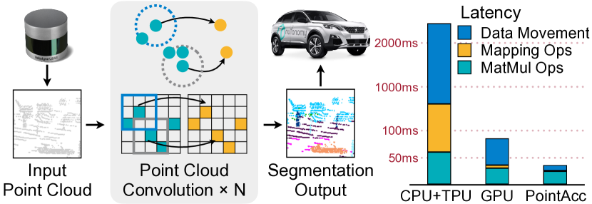
Figure 1. Point cloud deep learning is crucial for real-time AI applications. PointAcc accelerates point cloud computations by resolving sparsity and data movement bottlenecks.

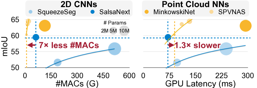
Figure 2. Compared to 2D CNNs, point cloud networks have higher accuracy and lower #MACs, but higher GPU latency due to low utilization brought by sparsity and irregularity.

1. Introduction

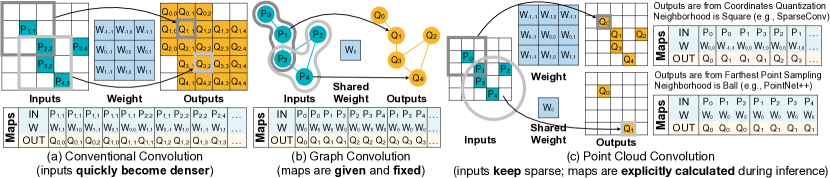
Figure 3. Convolution on point clouds (c) is very different from convolution on images (a) and graphs (b).

A point cloud is a collection of points that represent a physical object or 3D scene. Point clouds are usually generated by sensors like LiDARs at a rapid speed (2 million points per second for a 64-channel LiDAR sensor). As LiDARs are becoming as cheap as just hundreds of dollars, they are extensively deployed everywhere, in cars, robots, drones, and even in iPhone 12 Pros. Consequently, point clouds have become a modality as important as images and videos for deep learning applications such as autonomous driving, photography, virtual reality (VR), and augmented reality (AR). These applications require real-time interactions with humans, and thus it is crucial to emphasize not only high accuracy, but also low latency and energy consumption.

Compared to projecting 3D point cloud to 2D then applying Convolution Neural Networks (CNN) on 2D flattened point clouds (Figure 2 (left)), directly processing 3D point clouds with Point Cloud Networks (Qi et al., 2017b; Choy et al., 2019; Li et al., 2018; Wu et al., 2019; Wang et al., 2019; Li et al., 2021; Xu et al., 2018; Graham et al., 2018; Tang et al., 2020) yields up to 5% higher accuracy with 7$\times$ less #MACs. However, point cloud networks run significantly slower on existing general-purpose hardware than CNNs (Figure 2 right). The state-of-the-art point cloud model MinkowskiUNet (114G MACs) runs at only 11.7 FPS even on a powerful NVIDIA RTX 2080Ti GPU, while ResNet50 (He et al., 2016) (4G MACs) with similar input size can run at 840 FPS. To the best of our knowledge, the only accelerator for point cloud networks so far is Mesorasi (Feng et al., 2020). However, the “delayed aggregation” technique used by Mesorasi is restricted to only a small fraction of point cloud models, where all the neighbors are restricted to share the same weights. In contrast, state-of-the-art point cloud networks (Choy et al., 2019; Tang et al., 2020) use different weights for different neighbors, offering much higher accuracy. To tackle such dilemma, we present PointAcc, an efficient domain-specific accelerator for point cloud deep learning.

Computing on point clouds is challenging due to the high sparsity nature of inputs. For instance, outdoor LiDAR point clouds usually have a density of less than 0.01%, while traditional CNNs take in 100% dense images. Moreover, the sparsity in point clouds is fundamentally different from that in traditional CNNs which comes from the weight pruning and ReLU activation function. The sparsity in point clouds conveys physical information: the sparsity pattern is constrained by the physical objects in the real world. That is to say, the nonzero points will never dilate during the computation.

Therefore, point cloud processing requires a variety of mapping operations, such as ball query and kernel mapping, to establish the relationship between input and output points for computation, which has not been explored by existing deep learning accelerators. To tackle this challenge, PointAcc unifies these operations in a ranking-based computation paradigm which can generalize to other similar operations. By leveraging this shared computation paradigm, PointAcc further presents a versatile design to support diverse mapping operations on the arbitrary scale of point clouds. Moreover, strictly restricted sparsity pattern in point cloud networks leads to irregular sparse computation pattern. Thus it requires explicit gather and scatter of point features for matrix computation, which results in a massive memory footprint. To address this, PointAcc performs flexible control on on-chip memory using decoupled and explicit data orchestration (Pellauer et al., 2019). By caching the input features on demand with configurable block size and temporally fusing the computation of consecutive layers, PointAcc manages to improve the data reuse and reduce the expensive DRAM access.

In summary, this work makes the following contributions:

• We comprehensively investigate the datasets, computation cost and memory footprint of point cloud processing, and analyze the performance bottleneck on various hardware platforms. The sparsity of point cloud introduces unexplored mapping operations, and requires explicit gather/scatter.

• We present a versatile design to support diverse mapping operations that finds the nonzero neighbors and nonzero output point clouds corresponding to each weight. It unifies and converts the mapping operations into ranking-based comparisons. Our design manages to handle the arbitrary scales of point clouds.

• We present an efficient memory management design that decouples the memory request and response to precisely control the memory. It exploits caching and simplifies the layer fusion for point cloud networks, which reduces the DRAM access by up to 6.3$\times$.

We implement and synthesize PointAcc in TSMC 40nm technology node. Extensively evaluated with 8 modern point cloud networks on 5 datasets, PointAcc achieves an order of magnitude speedup on average compared with other hardware platforms. Co-designing the neural network, PointAcc outperforms the prior state-of-the-art point cloud accelerator Mesorasi by 100$\times$ speedup and 9.1% better mIoU accuracy running segmentation on the S3DIS dataset.

2. Background

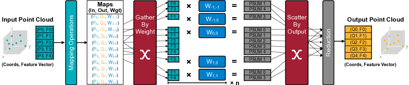
Figure 4. Existing CPU / GPU implementations for a point cloud convolution layer. Here $\bm{p}_{k}=(x_{k},y_{k},z_{k})$.

Table 1. Point Cloud Convolutions in Point Cloud Deep Learning.

Point Cloud Convolution	Mapping Operations		MatMul Operations
	Output Cloud Construction	Neighbor Search	Neighbor Aggregation
PointNet++-based	Farthest Point Sampling(Qi et al., 2017b; Li et al., 2018)	Ball Query (Qi et al., 2017b)	MaxPool (Qi et al., 2017b; Wang et al., 2019; Li et al., 2021)
(including Graph-based)	Random Sampling (Li et al., 2018)	k Nearest Neighbors(Li et al., 2018; Wang et al., 2019; Li et al., 2021; He et al., 2020)	Convolution1d (Li et al., 2018)
SparseConv-based	Coordinates Quantization	Kernel Mapping	Accumulation
(Graham et al., 2018; Choy et al., 2019; Tang et al., 2020; Han et al., 2020; Shi et al., 2021; Cheng et al., 2021; Yin et al., 2021)			(i.e., Convolution3d)

Point Cloud is a set of points $\bm{x}=\{\bm{x}_{k}\}=\{(\bm{p}_{k},\bm{f}_{k})\}$, where $\bm{p}_{k}=(x_{k},y_{k},z_{k})$ is the coordinate of the $k$^th point, and $\bm{f}_{k}$ is the corresponding 1-D feature vector. The key component of point cloud networks is the point cloud convolution. We compare convolution on different modalities in Figure 3, where the green grids/dots are (nonzero) inputs and the yellow ones are outputs.

Similar to image convolution which works on the receptive field (Figure 3a), point cloud convolution is conducted on the neighborhood of the output point (Figure 3c). Intuitively, if a input point $\bm{p}_{j}$ is the $n$-th neighbor of output point $\bm{q}_{k}$, we will perform $\bm{psum}_{k}$+=$\bm{f}_{j}\bm{w}_{n}$, where $\bm{w}_{n}$ is the corresponding weights. We define such relationship between input and output point as a map, i.e., map is a tuple $(\bm{p}_{j},\bm{q}_{k},\bm{w}_{n})$. Point cloud convolution iterates over all maps and performs multiplication-accumulation accordingly. Note that maps in image convolution can be directly inferred by pointer arithmetic since image pixels are dense (Figure 3a), and maps in graph convolution (Figure 3b) are provided as the adjacency matrix and stay constant across layers. However, maps in point cloud convolution have to be explicitly calculated every time downsampling the point cloud, due to the sparse nature of point clouds. In addition, for different neighbors, graph convolutions use the same weights, while state-of-the-art point cloud convolutions use different weights.

The state-of-the-art CPU/ GPU implementation of point cloud convolution is summarized in Figure 4. Specifically, we first perform mapping operations to find the input-output maps. Based on these maps, we gather the input features for different weights, transform features via matrix multiplication, and then scatter-aggregate the partial sums to the corresponding output points. The entire computation process consists of three types of operations: mapping, data movement (gather/scatter) and matrix multiplication (MatMul), as summarized in Table 1. We categorize point cloud convolutions into two classes: PointNet++-based and SparseConv-based convolutions. Graph-based convolutions (Wang et al., 2019; Li et al., 2021; He et al., 2020) are treated as the special case of PointNet++-based convolution, where the mapping operations work on the point features instead of point coordinates.

2.1. Mapping Operations

Mapping is the procedure to find the input-output maps $\mathcal{K}$ in point clouds, where $\mathcal{K}=\{(\bm{p}_{j},\bm{q}_{k},\bm{w}_{n})\}$. The search for maps runs two tasks: output point cloud construction and neighbor search (Table 1). These operations usually only take point coordinates as input.

2.1.1. Output Point Cloud Construction

The coordinates of output points are explicitly calculated during downsampling. Upsampling the point cloud is the inverse of corresponding downsampling.

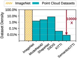
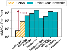
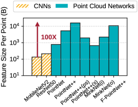
Figure 5. Point cloud datasets are ultra sparse. Point cloud networks have large computation cost and memory footprint.

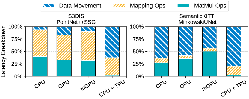
Figure 6. Point cloud networks are bottlenecked by data movement and mapping operations.

Coordinates Quantization. SparseConv-based convolution directly reduces the point cloud resolution during the downsampling. Specifically, the output point coordinate is calculated by quantization: $\bm{q}=\texttt{floor}(\bm{p}/ts)\times ts$, where $ts$ is the tensor stride ($ts=2^{k}$ after $k$ downsamplings). For example, point $(3,5)$ whose $ts=1$ will be quantized to $(2,4)$ whose $ts=2$ after downsampling, and point $(4,8)$ whose $ts=4$ will be quantized to $(0,8)$ whose $ts=8$ after downsampling. Such quantization can be easily implemented on hardware by clearing the lowest $\log_{2}(ts)$ bits of coordinates.

Farthest Point Sampling. PointNet++-based convolution applies farthest point sampling during the downsampling, where each output point is sampled from the input point cloud $I$ one by one iteratively. In each iteration $t$, we choose the point that has the largest distance to the current output point cloud $O_{t}$. For example, in Figure 3c (bottom), we select $\bm{q}_{0}$ as the first output point, and since $\bm{q}_{4}$ is farthest from $\bm{q}_{0}$, we select it as the second output point.

2.1.2. Neighbor Search

For each output point, the neighbor search is performed in the input point cloud to generate the maps.

Kernel Mapping. In SparseConv-based convolution, each output point will travel through all its neighborhood positions with offsets $\bm{\delta}\in\{-1,0,1\}^{D}$, where $D$ is dimension of the point cloud ($D=2$ in Figure 3). In Figure 3c, output point $\bm{q}_{0}$ has neighbor $\bm{p}_{0}$ with offset $(0,0)$ and neighbor $\bm{p}_{1}$ with offset $(1,1)$. Hence, maps $(\bm{p}_{0},\bm{q}_{0},\bm{w}_{0,0}),(\bm{p}_{1},\bm{q}_{0},\bm{w}_{1,1})$, are generated.

k-Nearest-Neighbors and Ball Query. In PointNet++-based convolution, based on the distances to output point $\bm{q}$, top-k input points $\bm{p}$ are selected. Ball query further requires these points to lie in the sphere of radius $r$ , i.e., $||\bm{p}-\bm{q}||_{2}\leq r$. In Figure 3c (bottom), there are three maps associated with $\bm{q}_{0}$, and four maps for $\bm{q}_{1}$.

2.2. MatMul Operations

MatMul operations are conducted on features $\bm{f}$ based on the maps. Specifically, we group all input features associated with the same weight $\bm{w}_{n}$ (i.e. gather by weight) and use one (Choy et al., 2019) or several FC layers (Qi et al., 2017b) to obtain partial sums $\bm{psum}=\bm{f}\cdot\bm{w}_{n}$. The partial sums are later aggregated (via max-pooling (Qi et al., 2017b), convolution (Li et al., 2018) or accumulation (Choy et al., 2019)) after being scattered to the corresponding output location (i.e. scatter by output). In Figure 4, we gather $[\bm{f}_{0},\bm{f}_{3}]$, multiply them with the weight matrix $\bm{w}_{-1,-1}$, and scatter-aggregate them to output $[\bm{f}_{1},\bm{f}_{4}]$ according to the maps. We then repeat the same process for $\bm{w}_{-1,0},...,\bm{w}_{1,1}$ sequentially.

3. Motivation

As shown in Figure 6 and Figure 6, we systematically profile the characteristics of point cloud datasets and networks, and their performance on various platforms, including CPU, GPU, mobile GPU, and TPU. We find that the challenge of accelerating point cloud networks comes from the intrinsic sparsity of the point cloud.

Challenge: High Input Sparsity. Unlike the input of image CNNs which are dense tensors, point cloud is naturally sparse. Figure 6 (left) plots the input sparsity of five mainstream point cloud datasets ModelNet40 (Wu et al., 2015), ShapeNet (Chang et al., 2015), KITTI (Geiger et al., 2012), S3DIS (Armeni et al., 2016) and SemanticKITTI (Behley et al., 2019), with details summarized in Table 2. Point clouds of 3D indoor scenes and objects have a density of $<10^{-2}$, and the 3D outdoor scenes are even sparser, reaching a density of less than $10^{-4}$. In contrast, ImageNet has 100% density at the input and 50% density on average after ReLU, which is up to four orders of magnitude denser than point cloud.

Conventionally, the input sparsity in CNNs results from the ReLU activation function. On the contrary, the sparsity in point cloud networks comes from the spatial distribution of the points, which contains the physical information in the real world. Therefore, it places hard constraint on the sparsity pattern in the point cloud convolution. In traditional sparse CNNs, the nonzero inputs are multiplied with every nonzero weights, and thus the nonzeros will dilate in the output. Such regular computation pattern is exploited in the prior sparse NN accelerators (Han et al., 2016; Parashar et al., 2017; Albericio et al., 2016; Zhang et al., 2016). However, in point cloud NNs, each nonzero input point is not always multiplied with all nonzero weights: the relationship among input points, weights and output points are determined by mapping operations. Hence previous sparse NN accelerators will not work.

Bottleneck I. New Operations: Mapping Operations. The first bottleneck due to point cloud sparsity is the mapping operations introduced in Section 2.1. As shown in Figure 6 (left), the PointNet++-based networks spend more than 50% of total runtime on mapping operations on general-purpose hardware platforms. Unfortunately, existing specialized NN accelerators do not support these mapping operations, and will worsen the performance. We take TPU (Jouppi et al., 2017) as an example. TPUs are tailored for dense matrix multiplications. Therefore, we have to first move all relevant data to host memory, rely on CPU to calculate the mapping operations and gather the features accordingly, and then send back the contiguous matrices to the TPU. Such a round trip between the heterogeneous memory can be extremely time-consuming. In practice, we found that the data movement time takes up 60% to 90% of total runtime.

Bottleneck II. Large Memory Footprint. The second bottleneck resulting from point cloud sparsity is the large memory footprint. Since the point cloud convolution has to explicitly gather input features and scatter partial sums, features can be repeatedly accessed for at most $3^{3}$=27 times (3D kernel with the size of 3). Moreover, in SparseConv-based models, downsampling only reduces the spatial resolution, and the number of points is usually not scaled down by 4$\times$ as in 2D CNNs. Therefore, the memory footprint of features in point cloud networks significantly surpasses CNNs. As shown in Figure 6 (right), the memory footprint of the features per point in point cloud networks can achieve up to 16 KB, which is 100$\times$ higher than CNNs. Thus the data movement alone can take up over 50% of total runtime on CPUs and GPUs, as shown in Figure 6 (right).

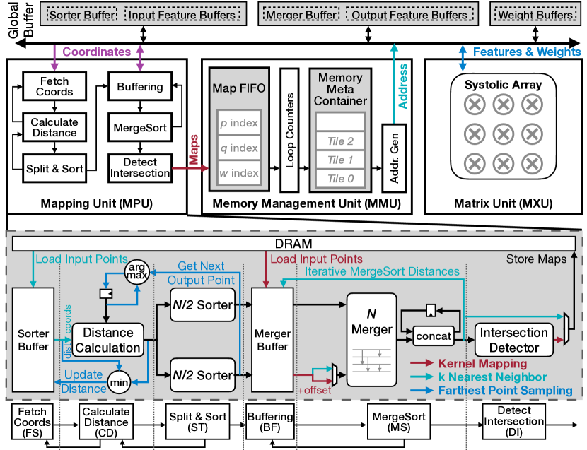
Figure 7. Overview of PointAcc Architecture.

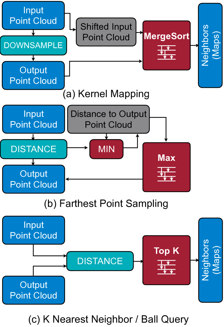
Figure 8. Mapping operations introduced by point cloud are unified to similar paradigm with ranking-based compute kernel.

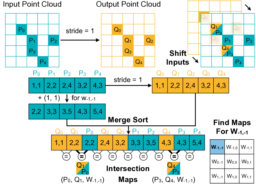
Figure 9. Mergesort-based Kernel Mapping Implementation.

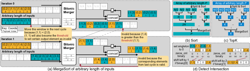
Figure 10. (a) Mapping Unit handles MergeSort of arbitrary length of inputs with forwarding loop; (b) Mapping Unit supports Sort of arbitrary length of inputs by iteratively MergeSort splited and sorted subarrays in a tree structure; (c) Mapping Unit flexibly realizes TopK on arbitrary length of inputs by truncating the intermediate merge-sorted subarrays to the length of k; (d) The intersection detector taking N elements has $\log N$ stages.

4. Architecture

To tackle the challenge discussed in Section 3, we present PointAcc architecture design, as shown in Figure 8. It consists of three parts: Mapping Unit, Memory Management Unit and Matrix Unit. Memory Management Unit bridges the other two units by preparing the data for Matrix Unit based on the output of Mapping Unit. By configuring the data flow in each unit, PointAcc flexibly supports various point cloud networks efficiently.

4.1. Mapping Unit

Conventional point cloud accelerators (Gieseke et al., 2014; Qiu et al., 2009; Heinzle et al., 2008; Winterstein et al., 2013; Xu et al., 2019; Feng et al., 2020) only focus on k-nearest-neighbors which is only one of mapping operations in the domain. Our Mapping Unit (MPU) targets all diverse mapping operations, including kernel mapping, k-nearest-neighbors, ball query and farthest point sampling. Instead of designing specialized modules for each possible operations, we propose to unify these diverse mapping operations into one computation paradigm, and convert them to point-cloud-agnostic operations, which can be further used to design one versatile specialized architecture.

4.1.1. Diverse Mapping Ops in One Architecture

The ultimate goal of mapping operations is to generate maps in the form of (input point index, output point index, weight index) tuple for further computation (e.g., convolution). We observe that no matter which algorithm is used, these maps are always constructed based on the comparison among distances. Thus we offer to convert these comparisons into ranking operations (Figure 8), and process in parallel for different points in the point cloud (point-level parallelism).

Farthest Point Sampling obtains the point in the input point cloud with the largest distance to the current output point cloud. We simply convert it to a Max operation on distances (Figure 8b).

k-Nearest-Neighbors searches k points in the input point cloud with smallest distances to the given output point, and ball query further requires these distances to be smaller than a predefined value. They can be implemented with TopK operation (Figure 8c).

Kernel Mapping can be regarded as finding the input points with the exact distance in the specific direction to the output points, i.e., finding the input point $p$ in the input point cloud $I=\{\bm{p}\}$ with certain offset $\delta$ to the output cloud $O=\{\bm{q}\}$, i.e. $\bm{p}=\bm{q}+\bm{\delta}$. For example, for the maps associating with weight $w_{-1,0}$, the input points are all right above the output points with distance of 1. Hence, the comparison is Equal operation on distances, which is done via the hash table in the state-of-the-art implementation (Tang et al., 2020). The hash table records the input point cloud coordinates, and each output point will query its possible neighbor from the table. A query hit indicates a map is founded. However, such hash-table-based solution is inefficient in terms of circuit specialization. On one hand, we cannot afford a large on-chip SRAM for the hash table which could be as large as 160 MB considering the input point cloud size and the load factor. On the other hand, even if we exploit the locality in the query process and build the hash table on the fly, we could not parallelize it efficiently. A parallelized hash table requires random parallelized read to the SRAM, which typically requires an $N$-by-$N$ crossbar with a space complexity of $O(N^{2})$.

Instead, we model the kernel mapping as finding the intersection on point coordinates between output point cloud $O$ and shifted input point cloud $I^{\prime}=\{\bm{p}-\bm{\delta}|\bm{p}\in I\}$. The parallelized Equal operation between two point clouds can be further converted to MergeSort of two point clouds (Figure 8c). The input point cloud $I$ is first applied the offset $-\bm{\delta}$, and then merge-sorted with the output point cloud $O$, which is an optionally downsampled version of the input cloud. The intersection can then be easily found by examining the adjacent elements, keeping those with the same coordinate and removing others. Experiment shows that our mergesort-based solution could provide 1.4$\times$ speedup while saving up to 14$\times$ area compared to the hash-table-based design with the same parallelism.

Example. Figure 9 illustrates an example where the input point cloud (green) is multiplied with the weight $w_{-1,-1}$. $\bm{\delta}=(-1,-1)$ for $w_{-1,-1}$; thus the input point cloud is shifted in the $(1,1)$ direction, i.e., the right-bottom direction. The shifting is performed by adding each coordinate with $-\bm{\delta}=(1,1)$. For example, $p_{0}=(1,1)$ becomes $(2,2)$ and $p_{1}=(2,2)$ becomes $(3,3)$. The shifted input cloud (green) are then merge-sorted with the output point cloud (yellow) which has the same coordinates as the input cloud since stride $s=1$, forming one sorted array. Each pair of adjacent elements in the array are fed to a comparator to see if their coordinates are equal. For instance, shifted $p_{0}$ and $q_{1}$ shares the same coordinates $(2,2)$, and thus they form a map $(p_{0},q_{1},w_{-1,-1})$. Here we found 2 maps.

4.1.2. Mapping Unit Architecture Design

As all mapping operations are converted to point-cloud-agnostic ranking operations (e.g., MergeSort, TopK in Figure 8), MPU exploits sorting-network-based design to support these ranking operations, and eliminates the data movement between co-processors as in TPU case in Figure 6.

We denote the comparator input element as ComparatorStruct which contains the comparator key (coordinates or distance) and the payload (e.g., the point index). As in Figure 8, MPU has 6 stages:

• FetchCoords (FS): fetch ComparatorStruct from sorter buffer; write back the updated distances forwarded from stage CD when running farthest point sampling (blue).

• CalculateDistance (CD): calculate the distances from input points to a specific output point; compare these distances with recorded distance in the payload and forward the minimum to the previous stage FS for farthest point sampling (blue).

• Sort (ST): split the outputs of stage CD into two sub-arrays, and sort them independently; compare the present maximum of sorter outputs with the history maximum in the register, and forward the final maximum to the previous stage CD after the traversal of the whole point cloud when executing farthest point sampling (blue).

• Buffering (BF): buffer the sorted arrays of ComparatorStruct from the previous stage ST or from the later stage MS when running k-nearest-neighbors (green).

• MergeSort (MS): merge-sort two arrays into one array (a forwarding loop is inserted inside the merger to handle arbitrary length of inputs); forward the results to the previous stage BF for sorting the arbitrary length of inputs when running k-nearest-neighbors (green).

• DetectIntersection (DI): detect the duplicate elements in the merged array as in Figure 10d. This stage is bypassed unless running kernel mapping (red).

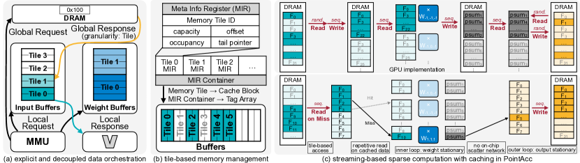
Figure 11. Memory Management Unit (MMU) design overview. (a) MMU exploits explicit and decoupled data orchestration (Pellauer et al., 2019). (b) MMU manages the on-chip memory in the granularity of “tile” (i.e., block). Its meta information (e.g., allocated capacity, starting address) is recorded in the Memory Tile Meta Info Register (MIR). (c) To handle the sparsity of point cloud convolution, MMU configures the input buffers as “cache” on demand, and stream the matrix computation without off-chip scattering.

4.1.3. MergeSort of Arbitrary Length.

An $N$-merger can only process a fixed-length array of $N$ elements, typically less than 64, which is far away from the size of point clouds ($10^{3}$-$10^{5}$ points). To handle such large scale, we add a forwarding loop after the merger. In each cycle, the merger takes in two arrays of $N/2$ elements but only consumes one array. Only first $N/2$ output elements are considered valid, and the rest $N/2$ elements are buffered for the next cycle.

Example. Figure 10a demonstrates how to achieve the MergeSort of arbitrary length. $N=8$ merger merges two input arrays of 4 elements. Thus, we apply a sliding window of size 4 on the input data before feeding to the merger.

At iteration 0, we feed the first 4 elements of both input (yellow) and output (green) point cloud to the merger. Meanwhile, both windows’ last elements are compared to determine whose window will be moved forward in the next cycle. Because coordinates (1,1) $<$ (2,0), the window on the output cloud will move forward. Since there could be elements larger than (1,1) but smaller (2,0) in the next cycle, all elements larger than (1,1) in the results should be discarded to ensure correctness. Therefore, (1,4) and (2,0) is marked as invalid by using (1,1) as a threshold. Since it is guaranteed that the merger consumes exactly one window (4 elements) in each iteration, we only output the first 4 elements of the merger results in each cycle. The rest 4 elements will be stored in the register to be used in the next cycle.

At iteration 1, we update the window of the output cloud (green) and keep that of the input cloud (yellow). As there are 2 valid elements we stored in the register in the last cycle, the first 2 elements of the current merger results are discarded and replaced by the elements from the last cycle.

4.1.4. Sort/TopK of Arbitrary Length.

A single pass of the first 5 stages in MPU without any forwarding works as a typical bitonic sorter. However, similar to the challenge in MergeSort mentioned above, to handle the arbitrary length of inputs, we perform a classical merge sort algorithm by forwarding the outputs of stage MS to stage FM and iteratively merge-sorting two sorted sub-arrays, as shown in Figure 10b. By truncating the intermediate subarrays to the length of k, MPU is able to directly support TopK with the same dataflow as running Sort operation as illustrate in Figure 10c.

Since the $k$ of TopK in point cloud models is usually very small (e.g., 16/32/64) compared to the size of input (e.g., 8192), the overhead of reusing sorter would be negligible. Experiment shows that on average our design is 1.18$\times$ faster than the quick-selection-based top-k engine proposed in SpAtten (Wang et al., 2021) with the same parallelism.

4.2. Memory Management Unit

As pointed out in Bottleneck II, explicit gather and scatter hinder the matrix computation. Therefore, we specialize the Memory Management Unit (MMU) to bridge the gap between computational resource needs and memory bound.

4.2.1. Data Orchestration

In point cloud networks, #layers of sparse computation (point cloud convolution) and dense computation (FC, convolution with kernel size of 1) are comparable. Among traditional memory idioms, workload-agnostic cache design is favoured for sparse computation, while workload-controlled scratchpad is popular for dense computation (Pellauer et al., 2019). To better handle both types of computation, MMU hybridizes two memory designs. MMU decouples the memory request initiator and response receiver (Figure 11a), and manages the on-chip buffers in the granularity of “tile” (Figure 11b). A memory tile contains the minimum memory space required for a computation tile of tiled matrix multiplication. The memory tile information such as address range and starting offset is exposed in the Memory Meta Info Register (MIR). Therefore, MMU is able to perform explicit and precise control over the memory space by manipulating the placement and replacement of MIRs in the MIR Container (Figure 11b): MMU will treat the MIR Container as a Tag Array when cache is needed for sparse computation, and as a FIFO or Stack when scratchpad is needed for dense computation.

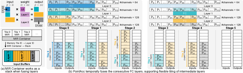
Figure 12. PointAcc temporally fuses the consecutive FC layers: (a) MIR Container is configured as a stack where different MIRs represent the data of different layers. (b) The data of current layer being computed are always at the top of the stack (e.g., Layer 2 in Stage 2). A memory tile is released if all the data are used (e.g., Layer 0 in Stage 1). If there are unused data for the previous layers, MIR only releases the used part (e.g., Layer 1 tile in Stage 2 is halved compared to that in Stage 1).

4.2.2. Data Flow

By reordering the computation loops of matrix multiplication, one can easily realize different data flow to improve the data reuse for inputs/weights/outputs. Since #points ($10^{3}\sim 10^{5}$) is much larger than the #channels ($10\sim 10^{3}$), even by orders of magnitude, we opt weight stationary data flow for inner computation loop nests to reduce on-chip memory accesses for weights. MMU will not increment input/output channels or neighbor dimension until it traverses all points in the on-chip buffers. Furthermore, we opt output stationary data flow for outer loop nests to eliminate the off-chip scatter of partial sums. MMU will not swap out the output features before it traverses all neighbors and all input channels.

4.2.3. MMU for Sparse Computation

As discussed in Section 2, MatMul computation in point cloud convolution is sparse and guided by the maps generated by Mapping Unit. Thus, in addition to computation loop counters, address generator will also require information from the maps, as shown in Figure 8 (top).

Optimize the Computation Flow. Computation flow affects memory behavior. The state-of-the-art GPU implementation will first gather all required input feature vectors, concatenate them as a contiguous matrix and then apply MM to calculate partial sums, referred as Gather-MatMul-Scatter flow. Contrarily, PointAcc calculates Matrix-Vector multiplication immediately after fetching the input features, referred as Fetch-on-Demand flow. As shown in Figure 11c, Fetch-on-Demand flow will save the DRAM access for input features by at least 3$\times$, by reducing the repetitive reads for gather and eliminating the writes after gather and reads for MM in the Gather-MatMul-Scatter flow.

Configure Input Buffers as Cache. In order to further reduce the repetitive reads of the same input point features in the Fetch-on-Demand flow, MMU configures the Input Buffers as a direct-mapped cache by reusing the MIR Container as a shared Tag Array recording the feature information.

Different from the traditional cache, contiguous entries in the input buffers are treated as a “cache block”, and thus the block size is software-controllable. The tag is composed of the point index and channel index of first input point inside the cache block. If both input point index and channel index of requested point features lie in the cache block size, a cache hit occurs. Otherwise, it is a cache miss and MMU will load the data block (i.e., a memory tile) containing the requested point features from DRAM.

Figure 20 shows the cache miss rate under fetch-on-demand mode running SparseConv of different parameters, where k is the kernel size (i.e., #neighbors) and c is the #channels. Both higher #neighbors and #channels improve the input features’ chances of being reused, and thus lower the cache miss rate. Meanwhile, as cache block size increases, the cache miss rate decreases as well but saturates at different points for different convolution parameters. Since a larger block size requires a longer latency to load from DRAM (i.e., a larger miss penalty), MMU is configured with different block sizes when running different SparseConv layers.

4.2.4. MMU for Dense Computation

For FC layers and convolutions with kernel size of 1, the matrix computation is dense and the input features are already contiguous in the DRAM. Thus, MMU only queries the MIR Container at the very beginning of each computation loop tile, reading out the MIR of current til and trying to allocate the memory and prefetch the data for next computation tile. A memory tile will be evicted (i.e., release) only when it conflicts with the prefetching tile. Hence, data will stay on-chip as long as possible, and be reused as much as possible.

Layer Fusion. PointAcc is able to fuse the computation of consecutive FCs in the point cloud convolution (Section 2.2) to further eliminate the DRAM accesses of the intermediate features. The conventional layer fusion (Alwani et al., 2016) spatially pipelines the computation, and thus fixes the number of fused layers and requires matching throughput in between. However, the number of consecutive layers varies among different models and even among different blocks in the same model. MMU thus temporally fuses these computation by simply configuring the MIR Container works as Stack and identifying the MIR by the layer index. The Matrix Unit always works with the top entry of MIR Container. When switching back to the previous unfinished layer, MIR Container will pop the top entry.

For FCs in the point cloud models, the point dimension can be regarded as the batch size dimension in traditional CNN. Thus, MMU can simplify the layer fusion logic by tiling the point dimension only without any halo elements between tiles. The number of fused layers and their tilings are determined during the compilation to avoid memory overflow. For each set of consecutive FCs, we will try to fuse all unprocessed FCs. If the estimated memory of required intermediate data overflows for all possible tilings, we will discard the last layer and try to fuse remaining ones. Such process is repeated until all layers are processed.

Example. Figure 12b shows an example of PointAcc fusing 3 consecutive FC layers.

• Stage 0: MMU loads features of $p_{0}$ to $p_{63}$ of layer 0 from DRAM.

• Stage 1: the computation in Stage 0 used up all loaded data and thus layer 0 tile is released. Switching to layer 1, MMU pushes features of layer 1 from Output Buffers.

• Stage 2: since layer 1 computation only uses half of input features ($p_{0}$ to $p_{31}$), the layer 1 tile capacity is halved. Switching to layer 2, MMU pushes features of layer 2 similar to Stage 1.

• Stage 3: since layer 2 is the last fused layer, we switch back to the previous layer (layer 1) after MMU pops layer 2 data. Since layer 1 tile capacity is nonzero, we continue to compute layer 1 for the rest features ($p_{32}$ to $p_{63}$).

• Stage 4: layer 1 tile is released since all data are used. Switching to layer 2, MMU pushes features of layer 2 similar to Stage 2.

• Stage 5: after finishing layer 2 and switching back to layer 1, we find that layer 1 tile capacity is zero. Thus we continue switching back to layer 0. Since layer 0 tile capacity is also zero, we will update outer loop counters, and then continue to work on layer 0 for the next tile $p_{64}$ to $p_{127}$.

4.3. Matrix Unit

Matrix Unit (MXU) adopts the classic systolic array as the computing core, since it has been proven to be efficient and effective for dense matrix multiplication. In order to completely eliminate the scatter network on-chip, MXU parallelizes the computation in input channels (ic) and output channels (oc) dimensions: each row of PEs computes in ic and each column of PEs computes in oc dimension independently. Thus, MXU only accesses features of one output point in one cycle, no more spatially scattering different points at one time and thus no need for the scatter circuit.

Table 2. Evaluation Benchmarks

Application	Dataset	Scene	Model	Notation
Classification	ModelNet40 (Wu et al., 2015)	Object	PointNet (Qi et al., 2017a)	PointNet
			PointNet++ (SSG) (Qi et al., 2017b)	PointNet++(c)
Part	ShapeNet (Chang et al., 2015)	Object	PointNet++ (MSG) (Qi et al., 2017b)	PointNet++(ps)
Segemantation			DGCNN (Wang et al., 2019)	DGCNN
Detection	KITTI (Geiger et al., 2012)	Outdoor	F-PoinNet++ (Qi et al., 2018)	F-PointNet++
Segemantation	S3DIS (Armeni et al., 2016)	Indoor	PointNet++ (SSG) (Qi et al., 2017b)	PointNet++(s)
			MinkowskiUNet (Choy et al., 2019)	MinkNet(i)
	SemanticKITTI (Behley et al., 2019)	Outdoor	MinkowskiUNet (Choy et al., 2019)	MinkNet(o)

Table 3. Evaluated ASIC platforms

Chip	Mesorasi	PointAcc	PointAcc.Edge
Cores	16$\times$16=256	64$\times$64=4096	16$\times$16=256
SRAM (KB)	1624	776	274
Area (mm2)	-	15.7	3.9
Frequency	1GHz	1 GHz	1 GHz
DRAM	LPDDR3-1600	HBM 2	DDR4-2133
Bandwidth	12.8 GB/s	256 GB/s	17 GB/s
Technology	16 nm	40 nm	40 nm
Peak Performance	512 GOPS	8 TOPS	512 GOPS

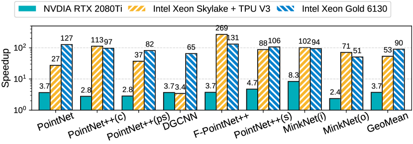
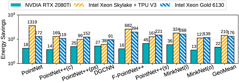
Figure 13. Performance gain over the server products: PointAcc is 3.7$\times$ faster than RTX 2080Ti on average.

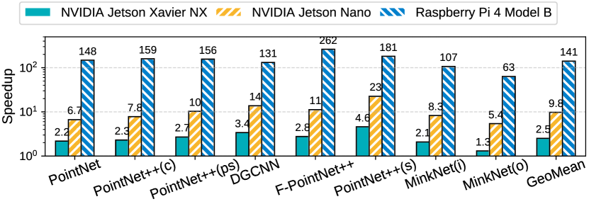
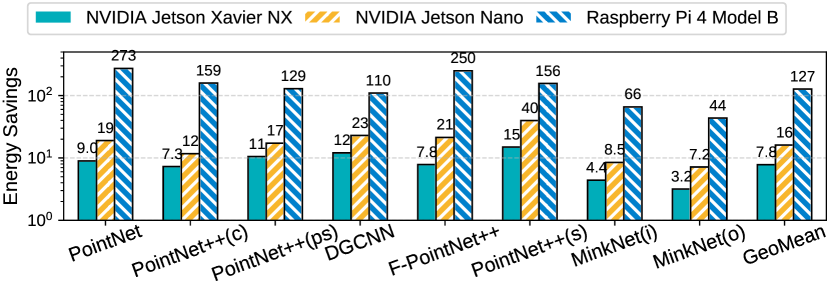
Figure 14. Performance gain over the edge devices: PointAcc.Edge is 2.5$\times$ faster than Jetson NX on average.

5. Evaluation

5.1. Evaluation Setup

Benchmarks. We pick 8 diverse point cloud network benchmarks across assorted application domains, including object classification, part segmentation, detection, and semantic segmentation. As shown in Table 2, the networks include both classical and state-of-the-art ones and cover all categories in Table 1. The selected datasets also contain various sizes and modalities for input point clouds, from daily objects to indoor scenes to spacious outdoor scenes. Such extensive benchmarks allow us to evaluate PointAcc thoroughly.

Hardware Implementation. We implement PointAcc with Verilog and verify the design through RTL simulations. We synthesize PointAcc with Cadence Genus under TSMC 40nm technology. Power of PointAcc is simulated with fully annotated switching activity generated with the selected benchmarks. We develop a cycle-accurate simulator to model the exact behavior of the hardware and calculate the cycle counts and read/write of on-chip SRAMs. The simulator is also verified against the Verilog implementation. We integrate the simulator with Ramulator (Kim et al., 2015) to model the DRAM behaviors. We obtain SRAM energy with CACTI (Muralimanohar et al., 2015), and DRAM energy using Ramulator-dumped DRAM commands trace.

Baselines. We adopt three kinds of hardware platforms as evaluation baselines: server-level products, edge devices, and a specialized ASIC design. For server-level products, we compare full-size PointAcc against Xeon^®  6130 CPU, RTX 2080Ti GPU, and TPU-v3. For edge devices and specialized ASIC, we compare the edge configuration (PointAcc.Edge) against Jetson Xavier NX, Jetson Nano, Raspberry Pi 4B, and Mesorasi (Feng et al., 2020) with NPU of 16$\times$16 systolic array. ASIC design parameters are compared in Table 3.

We implement point cloud networks with PyTorch (matrix operations with Intel MKLDNN / cuDNN, and mapping operations with C++ OpenMP / custom CUDA kernels). Our implementation achieves 2.7$\times$ speedup over the state-of-the-art implementaion MinkowskiEngine (Choy et al., 2019).

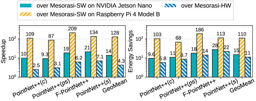
Figure 15. Speedup and energy savings of PointAcc.Edge over Mesorasi. Mesorasi-SW runs Mesorasi networks without specialized architectural support; Mesorasi-HW executes Mesorasi networks with dedicated aggregation unit AU and neural processing unit NPU.

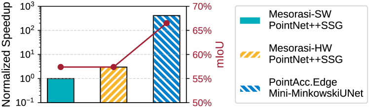
Figure 16. Mesorasi does not support independent weights for different neighbors, which is crucial in some variants of PointNet++-based blocks (Qi et al., 2017b) or SparseConv-based blocks (Choy et al., 2019). When running the same segmentation task on S3DIS dataset, PointAcc.Edge is able to execute networks with 10% higher accuracy and 100$\times$ lower latency.

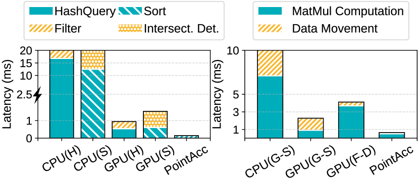
Figure 17. Latency breakdown of SparseConv-based blocks in operation level. Left: Kernel Mapping. Mergesort-based solution (S) runs slower than hash-table-based algorithm (H) on CPU/GPU, but 1.4$\times$ faster with 14$\times$ smaller area after circuit specialization (Section 4.1.1). Right: Convolution. Compared to the Gather-MatMul-Scatter flow (G-S), the reduction of data movement in Fetch-On-Demand flow (F-D) is dwarfed by the MV computation cost on GPU, but benefits PointAcc (Section 4.2.3).

5.2. Evaluation Results

5.2.1. Speedup and Energy Savings

Figure 14 presents the performance and energy benefits of PointAcc in comparison with GPU, TPU, and CPU products. On average, PointAcc offers 3.7$\times$, 53$\times$, 90$\times$ speedup and 22$\times$, 210$\times$, 176$\times$ energy savings, respectively. Figure 14 shows the speedup and energy savings of PointAcc.Edge over Jetson Xavier NX, Jetson Nano, and Raspberry Pi devices. On average, PointAcc.Edge achieves 2.5$\times$, 9.8$\times$, 141$\times$ speedup, and 7.8$\times$, 16$\times$, 127$\times$ energy savings, respectively. The improvements are consistent on different benchmarks. For TPU V3, the considerable gain mainly comes from supporting mapping operations with share compute kernel design, thus significantly reducing the data movements to/from host CPU.

5.2.2. Comparison with Mesorasi Architecture

Figure 16 shows the runtime speedup and energy savings of PointAcc.Edge over Mesorasi designs on PointNet++-based benchmarks. PointAcc.Edge achieves 1.3$\times$ speedup and 11$\times$ energy savings over Mesorasi hardware design on average. Unlike our design, Mesorasi is limited since it does not support independent weights for different neighbors. It is crucial for many point cloud networks (Li et al., 2018; Choy et al., 2019; Tang et al., 2020; Wu et al., 2019), especially for SparseConv-based models which not only improve the accuracy but also are capable of processing large-scale point clouds. We compare PointAcc.Edge with Mesorasi for the same segmentation task on the indoor scene dataset S3DIS. We scale down the SparseConv-based state-of-the-art model MinkowskiUNet to a shallower, narrower version, denoted as Mini-MinkowskiUNet. Co-designed with the neural network, PointAcc.Edge delivers over 100$\times$ speedup and improves the mean Intersection-over-Unit (mIoU) accuracy by 9.1%.

5.2.3. Source of Performance Gain

Ranking-based conversion of mapping operations. Figure 17 (left) breaks down the latency of mapping operation (kernel mapping here) of the 1st downsampling SparseConv-based block on SemanticKITTI. The mergesort-based algorithm (Figure 9) even worsens the performance on CPU/GPU. But compared to CPU/GPU, PointAcc is over 10$\times$ faster. Our design provides enough parallelism for comparison-intensive merge sort, and eliminates the repetitive access on intermediate results by spatially pipelining the stages of merge sort and intersection detection. On CPU/GPU, detecting intersection costs almost 2$\times$ runtime than filtering the query miss on hash table, because the length of inputs of intersection detection is doubled due to the merge of input/output point clouds. Querying the hash table costs almost comparable time with merge sort on GPU. It is because the hash-table-based algorithm only needs one pass on the input, but most stages of bitonic merge require a scan of the input from GPU global memory.

Fetch-On-Demand computation flow. Figure 17 (right) breaks down the latency of the matrix multiplication (convolution here) of the 1st layer of MinkowskiUNet on SemanticKITTI. Fetch-On-Demand flow saves the memory footprint by 3$\times$ but decomposes the matrix-matrix multiplication into fragmentary matrix-vector multiplications, and thus significantly increases the overhead due to low utilization of GPU. However, such overhead is removed in PointAcc because of the computation power of the systolic array. Therefore, PointAcc spends almost comparable time on the whole operation against the MatMul computation part only in the Gather-MatMul-Scatter flow.

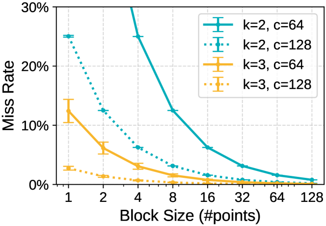
Figure 18. Miss rate of cache mode memory management. Miss rate decreases as cache block size, kernel size and #out_channels increases.

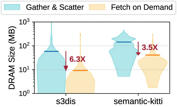
Figure 19. MinkowskiUNet layer DRAM access size distribution with and without caching. The bar denote the average DRAM access size per layer.

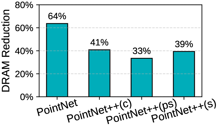
Figure 20. PointNet++ DRAM access size reduction of fusion mode memory management compared to running layer by layer independently.

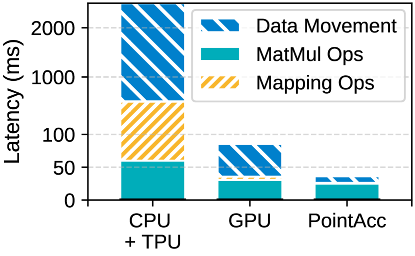
(a) Latency breakdown

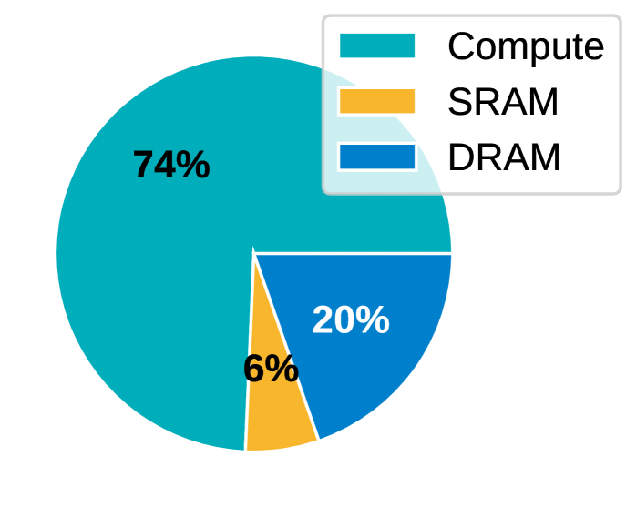
(b) Energy breakdown

Figure 21. Performance breakdown of PointAcc on MinkNet(o) benchmark: PointAcc reduces the latency and energy cost of data movement.

Configurable caching. Figure 20 demonstrates the distribution (i.e., probability density) of the DRAM access size per layer in MinkowskiUNet on S3DIS and SemanticKITTI dataset. A wider region indicates higher frequency of the given data size. The shape of distribution are nearly the same with/without caching, which indicates that the caching works consistently on different layers and on different datasets. On average, the configurable cache reduces the layer DRAM access by 3.5$\times$ to 6.3$\times$, where each point features are only fetched nearly once on average.

Temporal layer fusion. Figure 20 shows the reduction ratio of DRAM access when running PointNet++-based networks with Fusion Mode. Compared against running networks layer by layer independently, our simplified layer fusion logic help cut the DRAM access from 33% to 64%. Since there is no downsampling layers in PointNet, we are able to fuse more layers than other PointNet++-based networks, which leads to 1.5$\times$ to 2$\times$ more DRAM reduction.

Overall performance breakdown. Figure 21 breaks down the latency and energy consumption of PointAcc running MinkowskiUNet on SemanticKITTI dataset. The support of mapping operations gets rid of the extra cost on communication between co-processors as in CPU+TPU case. The specialized data orchestration in MMU helps reduce the DRAM access and make the data movement overlap the matrix multiplication. Therefore, the MatMul operations dominate the overall latency. Moreover, the computation covers 69% of total energy while DRAM access costs 23% of total energy, which differs from the observation in (Chen et al., 2016) where DRAM accesses dominate the energy consumption of FC layers.

6. Related Work

Deep Learning on Point Clouds. Early research converted point clouds to the volumetric representation and applied vanilla 3D CNNs (Qi et al., 2016) on the voxel grids. Qi et al. then proposed PointNet (Qi et al., 2017a) and its hierarchical version, PointNet++ (Qi et al., 2017b) to perform direct deep learning on point clouds. Later research such as Deep KD-Net (Klokov and Lempitsky, 2017), SpiderCNN (Xu et al., 2018), PointCNN (Li et al., 2018), PointConv (Wu et al., 2019), KPConv (Thomas et al., 2019) are variants of PointNet++. PVCNN (Liu et al., 2019) combined the advantages of point cloud and volumetric representations. Another stream of research SSCN (Graham et al., 2018), MinkowskiNet (Choy et al., 2019), SPVNAS (Tang et al., 2020) focus on SparseConv-based methods, which are more efficient than PointNet++-based methods on large outdoor scenes.

Point Cloud Accelerators. Researchers have extensively developed architectures and systems (Gieseke et al., 2014; Qiu et al., 2009; Heinzle et al., 2008; Winterstein et al., 2013; Xu et al., 2019) for accelerating neighbor search, especially for point cloud registration task. There has been limited work on point cloud deep learning. Feng et al. proposed Mesorasi, an architecture support for PointNet++-based networks via delayed-aggregation (Feng et al., 2020). However, Mesorasi has limited applicability as explained in Section 5.2.2.

Deep Learning Accelerators. Various work has explored both FPGA (Umuroglu et al., 2017) and ASIC (Chen et al., 2014; Chen et al., 2016; Shafiee et al., 2016; Zhang* et al., 2020; Wang et al., 2021) accelerator architectures for efficient DNN inference. EIE (Han et al., 2016), Cambricon-X (Zhang et al., 2016), Cnvlutin (Albericio et al., 2016) and SCNN (Parashar et al., 2017) exploited the sparsity in DNNs and speeded up the inference by skipping unstructured zeros. As discussed in Section 3, these conventional sparse accelerators do not support modern point cloud networks.

7. Conclusion

Moving from 2D images, machines start to perceive the world through 3D point clouds to recognize the world better. The rapid development of point cloud deep learning brings new challenges and exciting opportunities for intelligent hardware design. This work presents a specialized point cloud deep learning accelerator PointAcc, a new advancement that could help bring powerful point cloud AI to real-world applications, from augmented reality on iPhones to autonomous driving of intelligent vehicles, supporting real-time interactions with humans. PointAcc supports the newly introduced mapping operations by unifying and mapping them onto a shared ranking-based compute kernel. At the same time, PointAcc addresses the massive memory footprint problem due to the sparsity of point clouds by streaming the sparse computation with on-demand caching and temporally fusing the consecutive layers of dense computation. Extensive evaluation experiments show that PointAcc delivers significant speedup and energy reduction over CPU, GPU, and TPU. PointAcc paves the way for efficient point cloud recognition.

- (1)
- Albericio et al. (2016) Jorge Albericio, Patrick Judd, Tayler Hetherington, Tor Aamodt, Natalie Enright Jerger, and Andreas Moshovos. 2016. Cnvlutin: Ineffectual-neuron-free deep neural network computing. ACM SIGARCH Computer Architecture News 44, 3 (2016), 1–13.
- Alwani et al. (2016) M. Alwani, H. Chen, M. Ferdman, and P. Milder. 2016. Fused-layer CNN accelerators. In Proceedings of the 49th Annual IEEE/ACM International Symposium on Microarchitecture (MICRO). 1–12.
- Armeni et al. (2016) Iro Armeni, Ozan Sener, Amir R. Zamir, Helen Jiang, Ioannis Brilakis, Martin Fischer, and Silvio Savarese. 2016. 3D Semantic Parsing of Large-Scale Indoor Spaces. In IEEE/CVF Conference on Computer Vision and Pattern Recognition (CVPR).
- Behley et al. (2019) Jens Behley, Martin Garbade, Andres Milioto, Jan Quenzel, Sven Behnke, Cyrill Stachniss, and Juergen Gall. 2019. SemanticKITTI: A Dataset for Semantic Scene Understanding of LiDAR Sequences. In IEEE/CVF International Conference on Computer Vision (ICCV).
- Chang et al. (2015) Angel X. Chang, Thomas Funkhouser, Leonidas Guibas, Pat Hanrahan, Qixing Huang, Zimo Li, Silvio Savarese, Manolis Savva, Shuran Song, Hao Su, Jianxiong Xiao, Li Yi, and Fisher Yu. 2015. ShapeNet: An Information-Rich 3D Model Repository. arXiv (2015).
- Chen et al. (2014) Yunji Chen, Tao Luo, Shaoli Liu, Shijin Zhang, Liqiang He, Jia Wang, Ling Li, Tianshi Chen, Zhiwei Xu, Ninghui Sun, et al. 2014. DaDianNao: A machine-learning supercomputer. In 2014 47th Annual IEEE/ACM International Symposium on Microarchitecture. IEEE, 609–622.
- Chen et al. (2016) Yu-Hsin Chen, Tushar Krishna, Joel S Emer, and Vivienne Sze. 2016. Eyeriss: An energy-efficient reconfigurable accelerator for deep convolutional neural networks. IEEE journal of solid-state circuits 52, 1 (2016), 127–138.
- Cheng et al. (2021) Ran Cheng, Ryan Razani, Ehsan Taghavi, Enxu Li, and Bingbing Liu. 2021. (AF)2-S3Net: Attentive Feature Fusion with Adaptive Feature Selection for Sparse Semantic Segmentation Network. In IEEE/CVF Conference on Computer Vision and Pattern Recognition (CVPR).
- Choy et al. (2019) Christopher Choy, JunYoung Gwak, and Silvio Savarese. 2019. 4D Spatio-Temporal ConvNets: Minkowski Convolutional Neural Networks. In IEEE/CVF Conference on Computer Vision and Pattern Recognition (CVPR).
- Feng et al. (2020) Yu Feng, Boyuan Tian, Tiancheng Xu, Paul Whatmough, and Yuhao Zhu. 2020. Mesorasi: Architecture Support for Point Cloud Analytics via Delayed-Aggregation. In 2020 53rd Annual IEEE/ACM International Symposium on Microarchitecture (MICRO). IEEE, 1037–1050.
- Geiger et al. (2012) Andreas Geiger, Philip Lenz, and Raquel Urtasun. 2012. Are we ready for Autonomous Driving? The KITTI Vision Benchmark Suite. In IEEE/CVF Conference on Computer Vision and Pattern Recognition (CVPR).
- Gieseke et al. (2014) Fabian Gieseke, Justin Heinermann, Cosmin Oancea, and Christian Igel. 2014. Buffer kd trees: processing massive nearest neighbor queries on GPUs. In International Conference on Machine Learning. 172–180.
- Graham et al. (2018) Benjamin Graham, Martin Engelcke, and Laurens van der Maaten. 2018. 3D Semantic Segmentation With Submanifold Sparse Convolutional Networks. In IEEE/CVF Conference on Computer Vision and Pattern Recognition (CVPR).
- Han et al. (2020) Lei Han, Tian Zheng, Lan Xu, and Lu Fang. 2020. OccuSeg: Occupancy-aware 3D Instance Segmentation. In IEEE/CVF Conference on Computer Vision and Pattern Recognition (CVPR).
- Han et al. (2016) Song Han, Xingyu Liu, Huizi Mao, Jing Pu, Ardavan Pedram, Mark A Horowitz, and William J Dally. 2016. EIE: efficient inference engine on compressed deep neural network. ACM SIGARCH Computer Architecture News 44, 3 (2016), 243–254.
- He et al. (2016) Kaiming He, Xiangyu Zhang, Shaoqing Ren, and Jian Sun. 2016. Deep Residual Learning for Image Recognition. In IEEE/CVF Conference on Computer Vision and Pattern Recognition (CVPR).
- He et al. (2020) Qingdong He, Zhengning Wang, Hao Zeng, Yi Zeng, Shuaicheng Liu, and Bing Zeng. 2020. SVGA-Net: Sparse Voxel-Graph Attention Network for 3D Object Detection from Point Clouds. arXiv preprint arXiv:2006.04043 (2020).
- Heinzle et al. (2008) Simon Heinzle, Gaël Guennebaud, Mario Botsch, and Markus Gross. 2008. A hardware processing unit for point sets. In Proceedings of the 23rd ACM SIGGRAPH/EUROGRAPHICS symposium on Graphics hardware. 21–31.
- Jouppi et al. (2017) N. P. Jouppi, C. Young, N. Patil, D. Patterson, G. Agrawal, R. Bajwa, S. Bates, S. Bhatia, N. Boden, A. Borchers, R. Boyle, P. Cantin, C. Chao, C. Clark, J. Coriell, M. Daley, M. Dau, J. Dean, B. Gelb, T. V. Ghaemmaghami, R. Gottipati, W. Gulland, R. Hagmann, C. R. Ho, D. Hogberg, J. Hu, R. Hundt, D. Hurt, J. Ibarz, A. Jaffey, A. Jaworski, A. Kaplan, H. Khaitan, D. Killebrew, A. Koch, N. Kumar, S. Lacy, J. Laudon, J. Law, D. Le, C. Leary, Z. Liu, K. Lucke, A. Lundin, G. MacKean, A. Maggiore, M. Mahony, K. Miller, R. Nagarajan, R. Narayanaswami, R. Ni, K. Nix, T. Norrie, M. Omernick, N. Penukonda, A. Phelps, J. Ross, M. Ross, A. Salek, E. Samadiani, C. Severn, G. Sizikov, M. Snelham, J. Souter, D. Steinberg, A. Swing, M. Tan, G. Thorson, B. Tian, H. Toma, E. Tuttle, V. Vasudevan, R. Walter, W. Wang, E. Wilcox, and D. H. Yoon. 2017. In-datacenter performance analysis of a tensor processing unit. In International Symposium on Computer Architecture (ISCA).
- Kim et al. (2015) Yoongu Kim, Weikun Yang, and Onur Mutlu. 2015. Ramulator: A fast and extensible DRAM simulator. IEEE Computer architecture letters 15, 1 (2015), 45–49.
- Klokov and Lempitsky (2017) Roman Klokov and Victor S Lempitsky. 2017. Escape from Cells: Deep Kd-Networks for the Recognition of 3D Point Cloud Models. In IEEE/CVF International Conference on Computer Vision (ICCV).
- Li et al. (2021) Guohao Li, Matthias Müller, Guocheng Qian, Itzel C. Delgadillo, Abdulellah Abualshour, Ali Thabet, and Bernard Ghanem. 2021. DeepGCNs: Making GCNs Go as Deep as CNNs. IEEE Transactions on Pattern Analysis and Machine Intelligence (PAMI) (2021).
- Li et al. (2018) Yangyan Li, Rui Bu, Mingchao Sun, Wei Wu, Xinhan Di, and Baoquan Chen. 2018. PointCNN: Convolution on -Transformed Points. In Advances in Neural Information Processing Systems (NeurIPS).
- Liu et al. (2019) Zhijian Liu, Haotian Tang, Yujun Lin, and Song Han. 2019. Point-Voxel CNN for Efficient 3D Deep Learning. In Advances in Neural Information Processing Systems (NeurIPS).
- Muralimanohar et al. (2015) Naveen Muralimanohar, Rajeev Balasubramonian, and Norman Jouppi. 2015. CACTI 6.0: A tool to model large caches. IEEE (2015).
- Parashar et al. (2017) Angshuman Parashar, Minsoo Rhu, Anurag Mukkara, Antonio Puglielli, Rangharajan Venkatesan, Brucek Khailany, Joel Emer, Stephen W Keckler, and William J Dally. 2017. SCNN: An accelerator for compressed-sparse convolutional neural networks. ACM SIGARCH Computer Architecture News 45, 2 (2017), 27–40.
- Pellauer et al. (2019) Michael Pellauer, Yakun Sophia Shao, Jason Clemons, Neal Crago, Kartik Hegde, Rangharajan Venkatesan, Stephen W Keckler, Christopher W Fletcher, and Joel Emer. 2019. Buffets: An Efficient and Composable Storage Idiom for Explicit Decoupled Data Orchestration. In Proceedings of the Twenty-Fourth International Conference on Architectural Support for Programming Languages and Operating Systems. ACM, 137–151.
- Qi et al. (2018) Charles R Qi, Wei Liu, Chenxia Wu, Hao Su, and Leonidas J Guibas. 2018. Frustum PointNets for 3D Object Detection from RGB-D Data. In IEEE/CVF Conference on Computer Vision and Pattern Recognition (CVPR).
- Qi et al. (2017a) Charles Ruizhongtai Qi, Hao Su, Kaichun Mo, and Leonidas J Guibas. 2017a. PointNet: Deep Learning on Point Sets for 3D Classification and Segmentation. In IEEE/CVF Conference on Computer Vision and Pattern Recognition (CVPR).
- Qi et al. (2016) Charles Ruizhongtai Qi, Hao Su, Matthias Niessner, Angela Dai, Mengyuan Yan, and Leonidas J. Guibas. 2016. Volumetric and Multi-View CNNs for Object Classification on 3D Data. In IEEE/CVF Conference on Computer Vision and Pattern Recognition (CVPR).
- Qi et al. (2017b) Charles Ruizhongtai Qi, Li Yi, Hao Su, and Leonidas J Guibas. 2017b. PointNet++: Deep Hierarchical Feature Learning on Point Sets in a Metric Space. In Advances in Neural Information Processing Systems (NeurIPS).
- Qiu et al. (2009) Deyuan Qiu, Stefan May, and Andreas Nüchter. 2009. GPU-accelerated nearest neighbor search for 3D registration. In International Conference on Computer Vision Systems. Springer, 194–203.
- Shafiee et al. (2016) Ali Shafiee, Anirban Nag, Naveen Muralimanohar, Rajeev Balasubramonian, John Paul Strachan, Miao Hu, R Stanley Williams, and Vivek Srikumar. 2016. ISAAC: A convolutional neural network accelerator with in-situ analog arithmetic in crossbars. ACM SIGARCH Computer Architecture News 44, 3 (2016), 14–26.
- Shi et al. (2021) Shaoshuai Shi, Li Jiang, Jiajun Deng, Zhe Wang, Chaoxu Guo, Jinaping Shi, Xiaogang Wang, and Hongsheng Li. 2021. PV-RCNN++: Point-Voxel Feature Set Abstraction With Local Vector Representation for 3D Object Detection. arXiv preprint arXiv:2102.00463 (2021).
- Tang et al. (2020) Haotian Tang, Zhijian Liu, Shengyu Zhao, Yujun Lin, Ji Lin, Hanrui Wang, and Song Han. 2020. Searching Efficient 3D Architectures with Sparse Point-Voxel Convolution. In European Conference on Computer Vision (ECCV).
- Thomas et al. (2019) Hugues Thomas, Charles R Qi, Jean-Emmanuel Deschaud, Beatriz Marcotegui, François Goulette, and Leonidas J Guibas. 2019. KPConv: Flexible and Deformable Convolution for Point Clouds. In IEEE/CVF International Conference on Computer Vision (ICCV).
- Umuroglu et al. (2017) Yaman Umuroglu, Nicholas J Fraser, Giulio Gambardella, Michaela Blott, Philip Leong, Magnus Jahre, and Kees Vissers. 2017. FINN: A framework for fast, scalable binarized neural network inference. In Proceedings of the 2017 ACM/SIGDA International Symposium on Field-Programmable Gate Arrays. 65–74.
- Wang et al. (2021) Hanrui Wang, Zhekai Zhang, and Song Han. 2021. SpAtten: Efficient Sparse Attention Architecture with Cascade Token and Head Pruning. In 2021 IEEE International Symposium on High Performance Computer Architecture (HPCA). IEEE.
- Wang et al. (2019) Yue Wang, Yongbin Sun, Ziwei Liu, Sanjay E. Sarma, Michael M. Bronstein, and Justin M. Solomon. 2019. Dynamic Graph CNN for Learning on Point Clouds. In ACM SIGGRAPH.
- Winterstein et al. (2013) Felix Winterstein, Samuel Bayliss, and George A Constantinides. 2013. FPGA-based K-means clustering using tree-based data structures. In 2013 23rd International Conference on Field programmable Logic and Applications. IEEE, 1–6.
- Wu et al. (2019) Wenxuan Wu, Zhongang Qi, and Li Fuxin. 2019. PointConv: Deep Convolutional Networks on 3D Point Clouds. In IEEE/CVF Conference on Computer Vision and Pattern Recognition (CVPR).
- Wu et al. (2015) Zhirong Wu, Shuran Song, Aditya Khosla, Fisher Yu, Linguang Zhang, Xiaoou Tang, and Jianxiong Xiao. 2015. 3D ShapeNets: A Deep Representation for Volumetric Shapes. In IEEE/CVF Conference on Computer Vision and Pattern Recognition (CVPR).
- Xu et al. (2019) Tiancheng Xu, Boyuan Tian, and Yuhao Zhu. 2019. Tigris: Architecture and algorithms for 3D perception in point clouds. In MICRO. 629–642.
- Xu et al. (2018) Yifan Xu, Tianqi Fan, Mingye Xu, Long Zeng, and Yu Qiao. 2018. SpiderCNN: Deep Learning on Point Sets with Parameterized Convolutional Filters. In European Conference on Computer Vision (ECCV).
- Yin et al. (2021) Tianwei Yin, Xingyi Zhou, and Philipp Krähenbühl. 2021. Center-based 3D Object Detection and Tracking. In IEEE/CVF Conference on Computer Vision and Pattern Recognition (CVPR).
- Zhang et al. (2016) Shijin Zhang, Zidong Du, Lei Zhang, Huiying Lan, Shaoli Liu, Ling Li, Qi Guo, Tianshi Chen, and Yunji Chen. 2016. Cambricon-X: An accelerator for sparse neural networks. In 2016 49th Annual IEEE/ACM International Symposium on Microarchitecture (MICRO). IEEE, 1–12.
- Zhang* et al. (2020) Zhekai Zhang*, Hanrui Wang*, Song Han, and William J Dally. 2020. Sparch: Efficient architecture for sparse matrix multiplication. In 2020 IEEE International Symposium on High Performance Computer Architecture (HPCA). IEEE, 261–274.