KiDS-1000 Cosmology: machine learning - accelerated constraints on Interacting Dark Energy with CosmoPower

Abstract

We derive constraints on a coupled quintessence model with pure momentum exchange from the public $\sim$1000 deg² cosmic shear measurements from the Kilo-Degree Survey and the Planck 2018 Cosmic Microwave Background data. We compare this model with $\Lambda$CDM and find similar $\chi^{2}$ and log-evidence values. We accelerate parameter estimation by sourcing cosmological power spectra from the neural network emulator CosmoPower. We highlight the necessity of such emulator-based approaches to reduce the computational runtime of future similar analyses, particularly from Stage IV surveys. As an example, we present MCMC forecasts on the same coupled quintessence model for a Euclid-like survey, revealing degeneracies between the coupled quintessence parameters and the baryonic feedback and intrinsic alignment parameters, but also highlighting the large increase in constraining power Stage IV surveys will achieve. The contours are obtained in a few hours with CosmoPower, as opposed to the few months required with a Boltzmann code.

1 INTRODUCTION

Current and forthcoming large-scale structure (LSS) surveys such as the Dark Energy Survey, ESA’s Euclid satellite mission, and the Vera C. Rubin Observatory’s Legacy Survey of Space and Time (VRO/LSST), are aiming to probe the nature of the dark sector (dark energy and dark matter) by performing high precision galaxy clustering and weak gravitational lensing measurements. The standard model of cosmology, $\Lambda$CDM, is currently providing the best fit to a suite of data from Cosmic Microwave Background (CMB) and LSS experiments (e.g. Aghanim et al. 2020b; Anderson et al. 2012; Song et al. 2015; Beutler et al. 2016; Tröster et al. 2020; Alam et al. 2021; Abbott et al. 2021; Heymans et al. 2021). $\Lambda$CDM assumes that dark energy is a cosmological constant, $\Lambda$, and that General Relativity describes gravity on all scales. It also assumes that dark energy and dark matter are non-interacting (uncoupled). LSS surveys are aiming to constrain exotic dark energy and modified gravity models (for reviews see e.g. Copeland et al. 2006; Clifton et al. 2012).

In this work we focus on constraining interacting dark energy (IDE) in the form of a scalar field $\phi$ (quintessence) explicitly coupled to cold dark matter (CDM). IDE models have been widely studied and have gained popularity as potential alternatives to $\Lambda$CDM (Amendola, 2000; Pourtsidou et al., 2013; Tamanini, 2015; Di Valentino et al., 2020; Lucca, 2021). Here we study a sub-class of models that only exhibit momentum exchange between dark energy and dark matter (Simpson, 2010; Pourtsidou et al., 2013; Baldi & Simpson, 2015, 2017; Chamings et al., 2020; Amendola & Tsujikawa, 2020; Kase & Tsujikawa, 2020). This allows them to fit CMB, supernovae, and baryon acoustic oscillation data very well (Pourtsidou & Tram, 2016; Linton et al., 2021), but they have not been tested yet with weak lensing data marginalising over baryonic feedback effects.

Baryonic and dark matter nonlinear effects become particularly important in weak lensing studies with Stage IV surveys like Euclid and VRO/LSST, as they dominate the small, nonlinear scales with the most constraining power (Schneider et al., 2020a; Schneider et al., 2020b; Martinelli et al., 2021). At the same time, the computational requirements for accurate parameter estimation are becoming very expensive. A typical Markov Chain Monte Carlo (MCMC) requires $>10^{4}$ evaluations of the theoretical model under consideration, with the runtime being dominated by the computation of cosmological power spectra with Boltzmann codes such as CAMB (Lewis et al., 2000) or CLASS (Lesgourgues, 2011; Blas et al., 2011). This has led to the development of fast power spectra emulators (e.g. Aricò et al., 2021; Mootoovaloo et al., 2022; Spurio Mancini et al., 2021) to accelerate the inference pipeline by replacing the Boltzmann code at each likelihood evaluation.

2 MODEL

The model we study belongs to the pure momentum transfer class of theories constructed in Pourtsidou et al. (2013); Skordis et al. (2015). Its main feature is that no coupling appears at the background level, regarding the fluid equations. This is in contrast to the most commonly considered coupled quintessence models, but it is also what makes this model able to fit data for a wide range of the coupling parameter $\beta$ (Pourtsidou & Tram, 2016). In addition, the energy-conservation equation remains uncoupled even at the linear perturbations level. Therefore, the model provides for a pure momentum-transfer coupling at the level of linear perturbations.

Following Pourtsidou & Tram (2016) we are going to concentrate on the case where the action for the scalar field $\phi$ is written as

$$S_{\phi} = \int dt\,d^{3}x\,a^{3}\left[\frac{1}{2}(1-2\beta)\dot{\phi}^{2}-\frac{1}{2}|\vec{\nabla}\phi|^{2}-V(\phi)\right]\,.$$

The model is physically acceptable for $\beta<\frac{1}{2}$. For $\beta\rightarrow 1/2$ there is a strong coupling pathology, while for $\beta>1/2$ there is a ghost in the theory since the kinetic term becomes negative.

2.1 Background Evolution

Assuming a flat Friedmann-Lemaître-Robertson-Walker (FLRW) Universe, the background energy density and pressure for quintessence are (Pourtsidou et al., 2013)

$$\bar{\rho}_{\phi}=\left(\frac{1}{2}-\beta\right)\frac{\dot{\bar{\phi}}^{2}}{a^{2}}+V(\phi);\;\;\bar{P}_{\phi}=\left(\frac{1}{2}-\beta\right)\frac{\dot{\bar{\phi}}^{2}}{a^{2}}-V(\phi)\,,$$ (1)

and the energy conservation equations are the same as in uncoupled quintessence:

$$\dot{\bar{\rho}}_{\phi}+3{\cal H}(\bar{\rho}_{\phi}+\bar{P}_{\phi})=0;\;\;\dot{\bar{\rho}}_{c}+3{\cal H}\bar{\rho}_{c}=0\,.$$ (2)

2.2 Linear Perturbations

In order to study the observational effects of the coupled models on the Cosmic Microwave Background and Large-Scale Structure (LSS), we need to consider linear perturbations around the FLRW background. The density contrast $\delta_{c}\equiv\delta\rho_{c}/\bar{\rho}_{c}$ obeys the standard evolution equation

$$\dot{\delta}_{c}=-k^{2}\theta_{c}-\frac{1}{2}\dot{h}.$$ (3)

The momentum-transfer equation depends on the coupling parameter, $\beta$, and is given by

$$\dot{\theta}_{c}=-{\cal H}\theta_{c}+\frac{(6{\cal H}\beta\bar{Z}+2\beta\dot{\bar{Z}})\varphi+2\beta\bar{Z}\dot{\varphi}}{a\left(\bar{\rho}_{c}-2\beta\bar{Z}^{2}\right)}\,,$$ (4)

where $\phi=\bar{\phi}+\varphi$, and $\bar{Z}=-\dot{\bar{\phi}}/a$. We implemented the above equations in class (Lesgourgues, 2011; Blas et al., 2011) in order to compute the CMB temperature and matter power spectra, following the previous implementation in Pourtsidou & Tram (2016). We fix the quintessence potential $V(\phi)$ to be the widely used single exponential form (1EXP)

$$V(\phi)=V_{0}e^{-\lambda\phi}.$$ (5)

Our initial conditions for the quintessence field are $\phi_{i}=10^{-4},\dot{\phi}_{i}=0$. However, the same cosmological evolution is expected for a wide range of initial conditions (Copeland et al., 2006).

2.3 Nonlinear effects

To exploit the constraining power of forthcoming large-scale structure datasets on IDE models it is crucial to accurately model nonlinear effects. N-body simulations for momentum exchange in the dark sector have been performed in Baldi & Simpson (2015, 2017), based on the elastic scattering model presented in Simpson (2010). However, for the model considered here there is no available non-linear prescription or N-body data. In our analysis we employ the nonlinear correction implemented in HMcode (Mead et al., 2021), which includes modelling of baryonic feedback effects. We remark that this prescription is based on the $\Lambda$CDM model. Following Spurio Mancini et al. (2019), we justify this choice with the expected limited impact of different nonlinear prescriptions on cosmological constraints from the KiDS dataset, given the range of scales probed. However, this approach will need to be modified for applications to future surveys, whose dark energy constraints will strongly depend on the nonlinear prescription adopted. We will return to this issue in section 5 in the context of IDE models, and discuss ways forward.

3 Data and methods

	Band Powers			COSEBIs			2PCFs			Planck
	$\Lambda$CDM	IDE	IDE ($\lambda=1$)	$\Lambda$CDM	IDE	IDE ($\lambda=1$)	$\Lambda$CDM	IDE	IDE ($\lambda=1$)	$\Lambda$CDM	IDE	IDE ($\lambda=1$)
$\Omega_{\mathrm{m}}$	$0.341_{-0.076}^{+0.057}$	$0.342_{-0.083}^{+0.065}$	$0.343_{-0.084}^{+0.049}$	$0.314_{-0.083}^{+0.057}$	$0.315_{-0.086}^{+0.067}$	$0.318_{-0.087}^{+0.049}$	$0.269_{-0.055}^{+0.030}$	$0.272_{-0.059}^{+0.034}$	$0.270_{-0.056}^{+0.027}$	$0.320_{-0.009}^{+0.009}$	$0.318_{-0.009}^{+0.009}$	$0.335_{-0.009}^{+0.009}$
$\sigma_{8}$	$0.714_{-0.105}^{+0.083}$	$0.714_{-0.107}^{+0.069}$	$0.722_{-0.106}^{+0.091}$	$0.743_{-0.095}^{+0.091}$	$0.745_{-0.090}^{+0.094}$	$0.751_{-0.114}^{+0.091}$	$0.816_{-0.068}^{+0.082}$	$0.812_{-0.068}^{+0.080}$	$0.830_{-0.073}^{+0.082}$	$0.813_{-0.008}^{+0.008}$	$0.814_{-0.008}^{+0.008}$	$0.790_{-0.008}^{+0.008}$
$S_{8}$	$0.749_{-0.023}^{+0.024}$	$0.751_{-0.023}^{+0.025}$	$0.760_{-0.029}^{+0.026}$	$0.747_{-0.019}^{+0.023}$	$0.751_{-0.019}^{+0.024}$	$0.760_{-0.028}^{+0.025}$	$0.765_{-0.019}^{+0.020}$	$0.765_{-0.019}^{+0.020}$	$0.780_{-0.029}^{+0.023}$	$0.839_{-0.017}^{+0.018}$	$0.839_{-0.017}^{+0.017}$	$0.835_{-0.015}^{+0.018}$
$\chi^{2}$	148.0036	148.2647	148.7240	77.9787	77.5061	78.4702	255.4080	256.4388	254.7876	980.7286	980.7316	980.5730
$\log\frac{\mathcal{Z}_{\mathrm{IDE}}}{\mathcal{Z}_{\Lambda\mathrm{CDM}}}$		$-0.055\pm 0.144$	$-0.240\pm 0.140$		$0.136\pm 0.146$	$-0.048\pm 0.148$		$-0.048\pm 0.183$	$0.151\pm 0.184$		$0.980\pm 0.277$	$0.402\pm 0.279$

Table 1: Mean and marginalised 68 per cent contours on key weak lensing parameters. We also report the $\chi^{2}$ and log-Bayes factors $\log\frac{\mathcal{Z}_{\mathrm{IDE}}}{\mathcal{Z}_{\Lambda\mathrm{CDM}}}$ values. For the LSS probes the log-Bayes factors are always smaller than 0.5 in absolute value; following Jeffreys (1961), these values indicate that neither of the two models is clearly favoured with respect to the other. The Planck value indicates the CMB data favour the IDE model, although not in a substantial way.

We consider the same $\sim$ 1000 deg² cosmic shear data from the KiDS survey (KiDS-1000) used in the recent analysis of Asgari et al. (2021, A21 in the following). Photometric redshift distributions, shear measurements and data modelling are the same presented in the KiDS-1000 papers (Hildebrandt et al. 2021; Giblin et al. 2021; Joachimi et al. 2021). As in A21, we consider three types of cosmic shear summary statistics, namely band powers (Schneider et al., 2002), Complete Orthogonal Sets of E/B-Integrals (COSEBIs, Schneider et al., 2010), and two-point real space correlation functions (2PCFs).

We sample the posterior distribution using the Python wrapper PyMultiNest (Buchner et al., 2014) of the nested sampler MultiNest (Feroz & Hobson, 2008), as embedded in MontePython (Brinckmann & Lesgourgues, 2018). We compare constraints obtained running the KiDS-1000 inference pipeline (for band powers, COSEBIs and 2PCFs) and the Planck 2018 TTTEEE+lowE joint polarisation and temperature analysis (Aghanim et al., 2020a). We use CosmoPower (Spurio Mancini et al., 2021, github) to replace the Boltzmann software Class in the computation of the matter and CMB power spectra. All contours shown in subsection 4.1 have been obtained with CosmoPower. An accuracy comparison between CosmoPower and Class contours is reported in subsection 4.2, where forecast contours are reported for a Stage IV survey configuration, obtained sourcing power spectra from CosmoPower and Class. The technical details of the neural network emulators are unchanged with respect to those described in Spurio Mancini et al. (2021).

Prior distributions for the sampled parameters are the same used in A21, with the addition of two uniform distributions for the IDE parameters $\beta\sim\mathcal{U}[-0.5,0.5]$ and $\mathrm{log}\,\lambda\sim\mathcal{U}[-3,0.32]$. We consider a uniform prior on $\mathrm{log}\,\lambda$ to account for the fact that $\lambda$ is not a dimensionless quantity (Mackay, 2003). Choosing uninformative priors is crucial to avoid obtaining constraints driven by the prior assumptions (Simpson et al., 2017; Heavens & Sellentin, 2018). We also report results obtained fixing $\lambda$ to 1 (Copeland et al., 1998). The covariance matrix is the same used in A21. Its analytical computation in $\Lambda$CDM is described in Joachimi et al. (2021); we do not recompute the covariance in the IDE scenario, because similarly to Spurio Mancini et al. (2019) we expect only a weak dependence of the theoretical predictions for the observables on the IDE parameters, verified by the weak constraints obtained on these parameters (see subsection 4.1).

4 Results

4.1 Constraints from KiDS-1000 and Planck

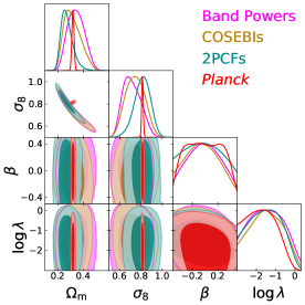
Figure 1 shows a comparison of marginalised 68 and 95 per cent contours of the posterior distribution for the key parameters $\Omega_{\mathrm{m}},\sigma_{8}$ and $S_{8}=\sigma_{8}\sqrt{\Omega_{\mathrm{m}}/0.3}$, as well as for the IDE parameters $\beta,\lambda$. As expected, the latter are unconstrained: differences in the matter power spectrum predictions for IDE models with respect to $\Lambda$CDM are mostly significant at highly nonlinear scales, only very mildly probed by the KiDS-1000 data. The Planck likelihood does not constrain $\beta$ and $\lambda$ either, in agreement with the fact that the CMB power spectra are essentially insensitive to these parameters, except on very large, cosmic variance - dominated scales (Pourtsidou & Tram 2016).

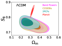
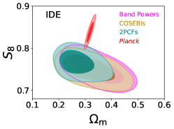
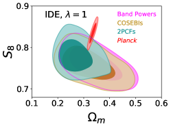
Table 1 shows the numerical values of the mean and 68 per cent credibility intervals for $\Omega_{\mathrm{m}},\sigma_{8}$ and $S_{8}$, along with $\chi^{2}$ and log-evidence values, for all cosmic shear summary statistics as well as for Planck. Figure 2 shows contours on the $\Omega_{\mathrm{m}}$-$S_{8}$ plane for the $\Lambda$CDM and IDE scenarios. The latter is analysed varying both $\beta$ and $\lambda$, as well as setting $\lambda=1$. With this last choice we find an attenuation of the tension up to $\sim$1$\sigma$. In Table 1 the $\chi^{2}$ and log-evidence values for $\Lambda$CDM and IDE scenarios (both varying and fixing $\lambda$) are similar across all three summary statistics, hence neither of the two cosmological models is clearly favoured over the other, although the Planck data seem to mildly prefer the IDE model over $\Lambda$CDM. Future analyses from Stage IV surveys will have the constraining power to provide stronger model comparison statements. It will be interesting to explore larger prior ranges for $\beta$, as well as different coupling functions, which may lead to stronger alleviation of the $S_{8}$ tension. For the KiDS-1000 data used in this paper we verified that larger, negative values of $\beta$ do not help alleviate the $S_{8}$ tension.

Figure 1: 68 and 95 per cent marginalised contours for key weak lensing parameters $\Omega_{\mathrm{m}},\sigma_{8},S_{8}$ and the IDE parameters $\beta,\lambda$. Contours for band powers, COSEBIs and two-point correlation functions are shown in magenta, brown and cyan, respectively, while Planck contours in red.

Figure 2: 68 and 95 per cent marginalised contours in the $\Omega_{\mathrm{m}}-S_{8}$ plane. The colour code is the same as in Fig. 1.

4.2 Forecasts for a Euclid-like survey

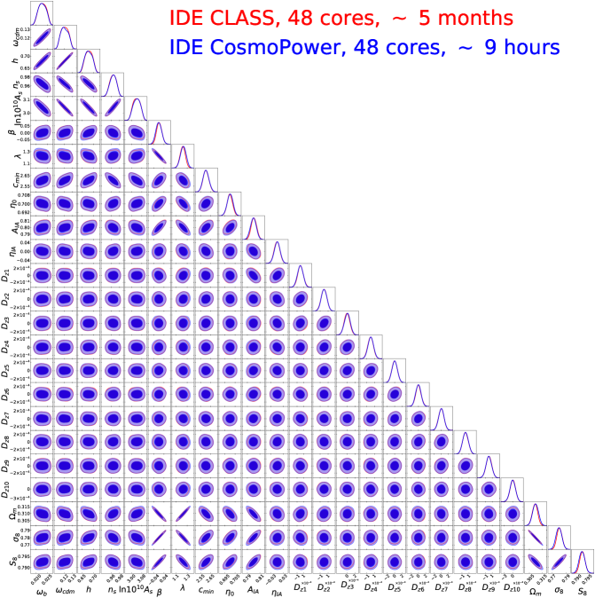
In Figure 3 we present forecast contours for a Euclid-like Stage IV survey. The simulated configuration is the same presented in Spurio Mancini et al. (2019), including the prior distributions on cosmological and astrophysical nuisance parameters. For the IDE parameters $\beta$ and $\lambda$, we use prior distributions $\beta\sim\mathcal{U}[-0.5,0.5]$ and $\lambda\sim\mathcal{U}[0.,2.1]$. We note that the prior on $\lambda$ differs from the one used for the KiDS-1000 data; for future analyses of real data from e.g. Euclid it will be important to consider a uniform prior on log$\,\lambda$ to account for the fact that $\lambda$ is not a dimensionless quantity (Mackay, 2003). Here, the goal is to highlight the importance of emulator-based approaches such as the one presented in this paper and based on CosmoPower. With this emulator, we obtained the contours for the Euclid-like survey (in blue in Figure 3) in $\sim$ 9 hours running on 48 cores. For comparison, sourcing power spectra from the Boltzmann code Class required a runtime of $\sim$ 5 months on the same hardware configuration (red contours in Figure 3).

We note that this Stage IV survey configuration leads to much stronger constraints on IDE parameters $\beta$ and $\lambda$, namely $\beta=-0.001_{-0.024}^{+0.023}$ and $\lambda=1.231_{-0.051}^{+0.054}$ (68 per cent contours). We also see that these IDE parameters are degenerate with nuisance parameters $A_{\mathrm{IA}}$ and $\eta_{\mathrm{IA}}$, modelling amplitude and redshift-dependence of the intrinsic alignment signal, respectively, as well as the HMcode parameters $c_{\mathrm{min}}$ and $\eta_{0}$, describing minimum halo concentration and halo bloating, respectively. These degeneracies highlight the importance of developing accurate prescriptions for nonlinearities and systematics that can guarantee unbiased constraints on dark energy.

Figure 3: Forecasts for a Euclid-like survey. The meaning of each parameter is explained in Spurio Mancini et al. (2021), whose analysis setup is identical to that considered here, with the sole addition of the interacting dark energy parameters $\beta$ and $\lambda$, introduced in section 2.

5 Conclusions

We presented constraints on an interacting dark energy (IDE) model from $\sim 1000$ deg² cosmic shear measurements from the Kilo-Degree Survey (KiDS-1000). A comparison with Planck measurements of the Cosmic Microwave Background (CMB) shows an alleviation up to $\sim$1$\sigma$ of the tension in the parameter $S_{8}=\sigma_{8}\sqrt{\Omega_{\mathrm{m}}/0.3}$, with respect to the $\sim 3\sigma$ tension of the $\Lambda$CDM analysis of Asgari et al. (2021). Constraints on the IDE model were obtained taking into account, for the first time, baryonic feedback effects. Given the absence of bespoke nonlinear prescriptions for IDE models, we adopted the $\Lambda$CDM-based nonlinear prescription implemented in the software HMcode. For applications to future surveys, proper nonlinear prescriptions for IDE models will need to be developed. We plan to consider the Elastic Scattering model and the halo model reaction framework (Cataneo et al., 2019; Bose et al., 2020; Tröster et al., 2021) for this purpose.

In deriving constraints, we used the neural network - based emulator of cosmological power spectra CosmoPower to accelerate the inference pipeline. We highlight the importance of such emulator-based approaches, in particular for applications to Stage IV surveys analyses. To demonstrate this point, we performed a forecast for a Stage IV Euclid-like survey for the same IDE model constrained with the KiDS-1000 data. Sourcing power spectra from CosmoPower allowed us to obtain contours in a few hours, while the same contours obtained using a Boltzmann code required a few months of run time.

The emulators trained for this analysis will remain available. For example, following Spurio Mancini et al. (2021), we emulated the linear matter power spectrum and a nonlinear boost. As new, bespoke nonlinear corrections for IDE models become available, the CosmoPower emulator for the nonlinear boost can be trained on them, while for the linear power spectrum we can reuse the emulator trained for this analysis.

Data Availability

KiDS-1000 data are available at http://kids.strw.leidenuniv.nl/DR4/lensing.php. The likelihood codes and emulators used in this analysis are shared on the CosmoPower GitHub repository github.

References

- Abbott et al. (2021) Abbott T. M. C., et al., 2021 (arXiv:2105.13549)
- Aghanim et al. (2020a) Aghanim N., et al., 2020a, Astronomy & Astrophysics, 641, A5
- Aghanim et al. (2020b) Aghanim N., et al., 2020b, Astron. Astrophys., 641, A6
- Alam et al. (2021) Alam S., et al., 2021, Phys. Rev. D, 103, 083533
- Amendola (2000) Amendola L., 2000, Phys.Rev., D62, 043511
- Amendola & Tsujikawa (2020) Amendola L., Tsujikawa S., 2020, JCAP, 06, 020
- Anderson et al. (2012) Anderson L., et al., 2012, Mon. Not. Roy. Astron. Soc., 427, 3435–3467
- Aricò et al. (2021) Aricò G., Angulo R. E., Zennaro M., 2021 (arXiv:2104.14568)
- Asgari et al. (2021) Asgari M., et al., 2021, Astronomy & Astrophysics, 645, A104
- Baldi & Simpson (2015) Baldi M., Simpson F., 2015, Mon. Not. Roy. Astron. Soc., 449, 2239
- Baldi & Simpson (2017) Baldi M., Simpson F., 2017, Mon. Not. Roy. Astron. Soc., 465, 653
- Beutler et al. (2016) Beutler F., et al., 2016, Mon. Not. Roy. Astron. Soc., 466, 2242–2260
- Blas et al. (2011) Blas D., Lesgourgues J., Tram T., 2011, JCAP, 07, 034
- Bose et al. (2020) Bose B., Cataneo M., Tröster T., Xia Q., Heymans C., Lombriser L., 2020, Mon. Not. Roy. Astron. Soc., 498, 4650
- Brinckmann & Lesgourgues (2018) Brinckmann T., Lesgourgues J., 2018 (arXiv:1804.07261)
- Buchner et al. (2014) Buchner J., et al., 2014, A&A, 564, A125
- Cataneo et al. (2019) Cataneo M., Lombriser L., Heymans C., Mead A., Barreira A., Bose S., Li B., 2019, Mon. Not. Roy. Astron. Soc., 488, 2121
- Chamings et al. (2020) Chamings F. N., Avgoustidis A., Copeland E. J., Green A. M., Pourtsidou A., 2020, Phys. Rev. D, 101, 043531
- Clifton et al. (2012) Clifton T., Ferreira P. G., Padilla A., Skordis C., 2012, Phys. Rept., 513, 1
- Copeland et al. (1998) Copeland E. J., Liddle A. R., Wands D., 1998, Phys. Rev. D, 57, 4686
- Copeland et al. (2006) Copeland E. J., Sami M., Tsujikawa S., 2006, Int. J. Mod. Phys. D, 15, 1753
- Di Valentino et al. (2020) Di Valentino E., Melchiorri A., Mena O., Vagnozzi S., 2020, Phys. Rev. D, 101, 063502
- Feroz & Hobson (2008) Feroz F., Hobson M. P., 2008, Mon. Not. Roy. Astron. Soc., 384, 449–463
- Giblin et al. (2021) Giblin B., et al., 2021, Astronomy & Astrophysics, 645, A105
- Heavens & Sellentin (2018) Heavens A. F., Sellentin E., 2018, Journal of Cosmology and Astroparticle Physics, 2018, 047–047
- Heymans et al. (2021) Heymans C., et al., 2021, Astronomy & Astrophysics, 646, A140
- Hildebrandt et al. (2021) Hildebrandt H., et al., 2021, Astronomy & Astrophysics, 647, A124
- Jeffreys (1961) Jeffreys S. H., 1961, Theory of Probability, 3 edn. Oxford
- Joachimi et al. (2021) Joachimi B., et al., 2021, Astronomy & Astrophysics, 646, A129
- Kase & Tsujikawa (2020) Kase R., Tsujikawa S., 2020, JCAP, 11, 032
- Kuijken et al. (2019) Kuijken K., et al., 2019, A&A, 625, A2
- Lesgourgues (2011) Lesgourgues J., 2011 (arXiv:1104.2932)
- Lewis et al. (2000) Lewis A., Challinor A., Lasenby A., 2000, ApJ, 538, 473
- Linton et al. (2021) Linton M. S., Crittenden R., Pourtsidou A., 2021 (arXiv:2107.03235)
- Lucca (2021) Lucca M., 2021, Phys. Dark Univ., 34, 100899
- Mackay (2003) Mackay D. J. C., 2003, Information Theory, Inference and Learning Algorithms
- Martinelli et al. (2021) Martinelli M., et al., 2021, Astron. Astrophys., 649, A100
- Mead et al. (2021) Mead A. J., Brieden S., Tröster T., Heymans C., 2021, Mon. Not. Roy. Astron. Soc., 502, 1401
- Mootoovaloo et al. (2022) Mootoovaloo A., Jaffe A. H., Heavens A. F., Leclercq F., 2022, Astron. Comput., 38, 100508
- Pourtsidou & Tram (2016) Pourtsidou A., Tram T., 2016, Phys. Rev. D, 94, 043518
- Pourtsidou et al. (2013) Pourtsidou A., Skordis C., Copeland E., 2013, Phys. Rev. D, 88, 083505
- Schneider et al. (2002) Schneider P., van Waerbeke L., Kilbinger M., Mellier Y., 2002, Astronomy & Astrophysics, 396, 1–19
- Schneider et al. (2010) Schneider P., Eifler T., Krause E., 2010, Astronomy and Astrophysics, 520, A116
- Schneider et al. (2020a) Schneider A., Stoira N., Refregier A., Weiss A. J., Knabenhans M., Stadel J., Teyssier R., 2020a, JCAP, 04, 019
- Schneider et al. (2020b) Schneider A., et al., 2020b, JCAP, 04, 020
- Simpson (2010) Simpson F., 2010, Phys. Rev. D, 82, 083505
- Simpson et al. (2017) Simpson F., Jimenez R., Pena-Garay C., Verde L., 2017, Journal of Cosmology and Astroparticle Physics, 2017, 029–029
- Skordis et al. (2015) Skordis C., Pourtsidou A., Copeland E., 2015, Phys. Rev. D, 91, 083537
- Song et al. (2015) Song Y.-S., et al., 2015, Phys. Rev. D, 92, 043522
- Spurio Mancini et al. (2019) Spurio Mancini A., et al., 2019, Mon. Not. Roy. Astron. Soc., 490, 2155
- Spurio Mancini et al. (2021) Spurio Mancini A., Piras D., Alsing J., Joachimi B., Hobson M. P., 2021 (arXiv:2106.03846)
- Tamanini (2015) Tamanini N., 2015, Phys. Rev. D, 92, 043524
- Tröster et al. (2020) Tröster T., et al., 2020, Astron. Astrophys., 633, L10
- Tröster et al. (2021) Tröster T., et al., 2021, Astron. Astrophys., 649, A88
- Wright et al. (2020) Wright A. H., Hildebrandt H., van den Busch J. L., Heymans C., 2020, A&A, 637, A100