Leading-Color Two-Loop Amplitudes for Four Partons and a $W$ Boson in QCD

Abstract

We present the leading-color two-loop QCD corrections for the scattering of four partons and a $W$ boson, including its leptonic decay. The amplitudes are assembled from the planar two-loop helicity amplitudes for four partons and a vector boson decaying to a lepton pair, which are also used to determine the planar two-loop amplitudes for four partons and a $Z/\gamma^{*}$ boson with a leptonic decay. The analytic expressions are obtained by setting up a dedicated Ansatz and constraining the free parameters from numerical samples obtained within the framework of numerical unitarity. The large linear systems that must be solved to determine the analytic expressions are constructed to be in Vandermonde form. Such systems can be very efficiently solved, bypassing the bottleneck of Gaussian elimination. Our results are expressed in a basis of one-mass pentagon functions, which opens the possibility of their efficient numerical evaluation.

1 Introduction

The production of a $W$ boson in association with jets is a key process at hadron colliders. It can be used for precise Standard-Model (SM) measurements and allows to constrain models beyond the SM. The $W+2$-jet signature is of particular interest, as it will play a distinguished role for future precision QCD analyses. By now, many observables for this process have already been measured at the LHC to 10% relative uncertainty ATLAS:2014fjg ; CMS:2017gbl , and substantial improvements are expected during Run 3 and the high-luminosity phase of the LHC. Theoretically this process stands out, because of the expected fast convergence in perturbation theory. Indeed, at this jet multiplicity all production channels are already contributing at Born level, with mild next-to-leading-order (NLO) QCD corrections over phase space and a small sensitivity to higher-order corrections Campbell:2003hd ; Berger:2009ep ; Anger:2017nkq ; Kallweit:2015dum ; Azzurri:2020lbf . The calculation of the corresponding next-to-next-to-leading-order (NNLO) QCD corrections is highly desirable, as it will allow to assess the quality of higher-order perturbative predictions in QCD DiGiustino:2020fbk ; Bonvini:2020xeo ; Duhr:2021mfd .

In this article we focus on the calculation of the two-loop scattering amplitudes necessary to obtain the leading-color NNLO QCD corrections for the production of a $W$ boson with two jets at hadron colliders. More precisely, we present the analytic form of the gauge-invariant planar contributions to the amplitudes for the scattering of four partons and a $W$ boson which decays into leptons. These amplitudes are the leading-color contributions corresponding to the formal large $N_{c}$ limit keeping the ratio $N_{f}/N_{c}$ fixed. We retain at the amplitude level the leptonic decay products of the vector boson, and consider all possible helicity configurations of the external particles. We focus on a representative physical kinematical channel for every amplitude that we compute. The presented amplitudes also give leading-color contributions for the scattering of four partons and a $Z/\gamma^{*}$ boson which decays into leptons, however, omitting the gauge invariant contributions originating from $Z/\gamma^{*}$ coupling directly to a closed quark loop.

While the one-loop helicity amplitudes for $e^{+}e^{-}\rightarrow 4$ partons have been known for more than two decades Bern:1997sc ; Bern:1996ka ; Glover:1996eh ; Campbell:1997tv , no analytic expression for corresponding two-loop scattering amplitudes has been available until now. Nevertheless there has been much related progress, first with a benchmark numerical evaluation of the amplitudes under consideration Hartanto:2019uvl and second with the computation of the two-loop squared amplitudes for the production of an on-shell $W$ boson in association with a $b\overline{b}$ pair Badger:2021nhg (see also related work on the two-loop helicity amplitudes for the production of a Higgs boson in association with a $b\overline{b}$ pair at the LHC Badger:2021ega ).

Progress in the field of two-loop scattering amplitudes in recent years has been substantial. This progress has been made on two fundamental aspects of their calculation. First, there have been important practical advances in understanding how to reduce scattering amplitudes to master integrals through so-called integration-by-pars (IBP) reduction Chetyrkin:1981qh ; Laporta:2000dsw . This has come both in the form of a better understanding of how to simplify IBP relations with unitarity-compatible techniques Gluza:2010ws ; Larsen:2015ped ; Ita:2015tya , as well as the suggestion to perform the reduction numerically over finite fields, and reconstruct the results from these evaluations vonManteuffel:2014ixa ; Peraro:2016wsq . By now a number of public implementations of reconstruction methodologies exist Klappert:2019emp ; Klappert:2020aqs ; Peraro:2019svx . In this context, an important advance has been the development of the multi-loop numerical unitarity method Ita:2015tya ; Abreu:2017xsl ; Abreu:2017hqn ; Abreu:2018zmy , where loop amplitudes are numerically computed by exploiting their analytic properties. On the second front, there has been a great deal of progress in understanding and computing the required master integrals, specifically in the framework of differential equations Kotikov:1990kg ; Remiddi:1997ny in their canonical form Henn:2013pwa . This powerful framework, when combined with Ansatz techniques Abreu:2018rcw , has led to the computation of not only the challenging planar two-loop five-point one-mass master integrals Papadopoulos:2015jft ; Abreu:2020jxa ; Canko:2020ylt relevant for the amplitudes discussed in this paper, but also the non-planar hexabox integrals Abreu:2021smk ; Papadopoulos:2019iam , which contribute for example to subleading color contributions. Bases of multi-valued transcendental functions contributing to five-point one-mass scattering have been constructed in refs. Badger:2021nhg ; Chicherin:2021dyp . These are an important ingredient enabling the application of modern techniques for the calculation of scattering amplitudes. Furthermore, there now exist multiple methodologies for the numerical evaluation of the integrals in the form of either generalized series expansions Moriello:2019yhu ; Hidding:2020ytt ; Abreu:2020jxa ; Badger:2021nhg , or iterated integral methods in the form of so-called pentagon functions Gehrmann:2018yef ; Chicherin:2020oor ; Chicherin:2021dyp .

In this work, we make use of these recent advances, employing and extending them to analytically compute for the first time the scattering amplitudes relevant for the leading-color production of a $W$ boson decaying to leptons in association with two jets at the LHC. In order to achieve this, we follow an Ansatz strategy, reconstructing the analytic form of the amplitudes from numerical samples over finite fields. The numerical reductions to master integrals are obtained with the numerical unitarity approach Ita:2015tya ; Abreu:2017xsl ; Abreu:2017hqn ; Abreu:2018zmy using the implementations within the Caravel framework Abreu:2020xvt . These numerical reductions, when combined with expressions for the master integrals in terms of a basis of pentagon functions Chicherin:2021dyp , allow us to subtract the known infrared Catani:1998bh ; Becher:2009cu ; Gardi:2009qi and ultraviolet pole contributions and perform a reconstruction of the so-called finite remainder. In order to efficiently perform the reconstruction, we describe a modern functional reconstruction algorithm. First we discuss how to map the six-point kinematics of the amplitudes including the $W$ boson decay to a lepton pair to the (six-scale) five-point one-mass kinematics which underlie the QCD corrections to the process. Then we discuss how we combine a univariate partial fraction approach Badger:2021nhg with an approach built on Vandermonde-based sampling Klappert:2019emp , resulting in a modern technique whose complexity is dominated by the sampling in the first finite field.

The paper is organized as follows. First, in section 2 we establish the notation to describe the amplitudes under consideration. Next, in section 3 we review the numerical aspects of the calculation framework and in section 4 we discuss the modern functional reconstruction approach employed to determine the analytic expressions. We then discuss implementation details and describe the analytic results in section 5. The analytic expressions are provided in an accompanying set of ancillary files W4partonsite . Finally, in section 6 we summarize the results of this paper. A series of appendices provide extra details of our calculation and results. trivial

2 Notation and Conventions

The main results of this paper are the leading-color two-loop QCD helicity amplitudes for the scattering of four partons and a $W$ boson, where the $W$ boson decays into a lepton pair. In the Standard Model, the $W$ boson couples with both vector and axial-vector couplings. However, it can be shown that if the $W$ boson always couples to a quark line connected to external states, as is the case in the amplitudes we consider, the vector and axial-vector contributions are equal up to an overall sign. We discuss this relation in more detail in appendix A. For now we simply note that this observation simplifies our computational setup. Indeed, it means that in order to assemble the amplitudes for four partons and a $W$ boson we can instead consider the amplitudes for four partons and a vector boson $V$ which only interacts through a vector (and not axial-vector) coupling.

Let us then consider the gauge-invariant planar contributions to the two-loop QCD helicity amplitudes for four partons and a vector boson $V$. The vector boson only interacts through a vector current, and decays into a lepton pair. There are two independent partonic processes to consider, one with a single quark line and one with two quark lines, and we assume the vector boson only couples to one of the quark flavors, which we denote as $\mathrm{q}$. In fig. 1 we schematically depict the two processes at tree level. The respective helicity amplitudes will be denoted as

$$\begin{split}&\mathcal{M}_{\mathrm{g}}\left(\bar{\mathrm{q}}^{h_{1}}_{p_{1}},\mathrm{g}^{h_{2}}_{p_{2}},\mathrm{g}^{h_{3}}_{p_{3}},\mathrm{q}^{h_{4}}_{p_{4}};\bar{\ell}^{h_{5}}_{p_{5}},{\ell}^{h_{6}}_{p_{6}}\right)\,,\\ &\mathcal{M}_{\mathrm{Q}}\left(\bar{\mathrm{q}}^{h_{1}}_{p_{1}},\mathrm{Q}^{h_{2}}_{p_{2}},\bar{\mathrm{Q}}^{h_{3}}_{p_{3}},\mathrm{q}^{h_{4}}_{p_{4}};\bar{\ell}^{h_{5}}_{p_{5}},{\ell}^{h_{6}}_{p_{6}}\right)\,,\end{split}$$ (1)

where $\mathrm{g}$ denotes a gluon, $\mathrm{q}$ and $\mathrm{Q}$ denote massless quarks which we assume have different flavors, and we have singled out the pair of leptons $\ell$ and $\bar{\ell}$ which are produced in the decay of the vector boson $V$. For each particle, we include a label $h_{i}$ to denote the helicity state and a label $p_{i}$ to denote the momentum. In this paper we will focus on the particular physical partonic channels where $p_{1}$ and $p_{2}$ are incoming. The complete set of partonic channels required for phenomenological applications can be obtained by a straightforward application of permutations of particles’ momenta, charge and parity conjugation (see discussion at the end of section 5.2).

From the amplitudes in LABEL:eq:partProcesses we can then assemble the amplitudes for Standard Model bosons. In particular, since the $W$ boson cannot couple directly to a closed fermion loop, the gauge-invariant planar contributions we consider in LABEL:eq:partProcesses capture the full leading-color contributions for the amplitudes for four partons and a $W$ boson decaying to leptons. Given that in this case the helicities of the emitting quark line and the leptons are fixed, we obtain, in all outgoing notation and closely following the notation of ref. Bern:1997sc ,

$$\begin{split}\mathcal{M}^{W}\left(\bar{u}_{p_{1}}^{R},g_{p_{2}}^{h_{2}},g_{p_{3}}^{h_{3}},d_{p_{4}}^{L},\bar{e}_{p_{5}}^{R},\nu_{p_{6}}^{L}\right)&=v^{2}\,{\cal P}_{W}(s_{56})\,\mathcal{M}_{\mathrm{g}}\left(\bar{q}^{+}_{p_{1}},g_{p_{2}}^{h_{2}},g_{p_{3}}^{h_{3}},{q}^{-}_{p_{4}};\bar{\ell}^{+}_{p_{5}},{\ell}^{-}_{p_{6}}\right)\,,\\ \mathcal{M}^{W}\left(\bar{u}_{p_{1}}^{R},c_{p_{2}}^{h},\bar{c}_{p_{3}}^{-h},d_{p_{4}}^{L},\bar{e}_{p_{5}}^{R},\nu_{p_{6}}^{L}\right)&=v^{2}\,{\cal P}_{W}(s_{56})\,\mathcal{M}_{\mathrm{Q}}\left(\bar{q}^{+}_{p_{1}},Q_{p_{2}}^{h},\bar{Q}_{p_{3}}^{-h},{q}^{-}_{p_{4}};\bar{\ell}^{+}_{p_{5}},{\ell}^{-}_{p_{6}}\right)\,,\end{split}$$ (2)

where $u$, $d$ and $c$ denote distinct quark flavours, and

$${\cal P}_{W}(s)=\frac{s}{s-M_{W}^{2}+\,\mathrm{i}\,\Gamma_{W}M_{W}}\,,\quad v^{2}=\frac{e^{2}}{2\sin^{2}{\theta_{w}}}\,.$$ (3)

$M_{W}$ is the mass of the $W$ boson, $\Gamma_{M}$ its decay width, $\theta_{w}$ is the Weinberg angle, and we assume a diagonal CKM matrix. For simplicity we only quote the result for quark lines from distinct families. The other combinations are obtained by suitable linear combinations. We will see in section 2.1 how the amplitudes in LABEL:eq:partProcesses can also be used to determine the planar gauge-invariant contributions for the amplitudes for four partons plus a $Z/\gamma^{*}$ decaying to leptons.

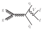
(a) Single quark line

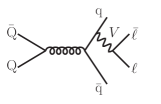
(b) Two quark lines

Figure 1: Schematic representation of the two partonic processes in eq. (LABEL:eq:partProcesses)

Having identified the amplitudes in LABEL:eq:partProcesses as the central building blocks, in the remaining of this paper we focus on their evaluation. The calculation of the loop amplitudes is performed in the ’t Hooft-Veltman (HV) scheme of dimensional regularization with $D=4-2\epsilon$ space-time dimensions. The dependence of all quantities on the dimensional regulator $\epsilon$ will in general be kept implicit. In dimensional regularization one must also take care with the precise definition of the helicity states of the external quarks, and we refer the reader to the detailed discussion in ref. Abreu:2018jgq where all our conventions are described.

The $\mathcal{M}_{\mathrm{g}}$ and $\mathcal{M}_{\mathrm{Q}}$ amplitudes can be expanded in powers of the bare coupling $\alpha_{s}^{0}=(g_{s}^{0})^{2}/(4\pi)$,

$$\mathcal{M}_{\kappa}=(g_{s}^{0})^{2}\left(\mathcal{M}_{\kappa}^{(0)}+\frac{\alpha_{s}^{0}}{2\pi}\mathcal{M}_{\kappa}^{(1)}+\left(\frac{\alpha_{s}^{0}}{2\pi}\right)^{2}\mathcal{M}_{\kappa}^{(2)}+\mathcal{O}\left(\left(\alpha_{s}^{0}\right)^{3}\right)\right)\,,\qquad\textrm{for }\kappa=\mathrm{g},\,\mathrm{Q}\,.$$ (4)

The tree level $\mathcal{M}_{\kappa}^{(0)}$ and one-loop $\mathcal{M}_{\kappa}^{(1)}$ contributions are known Bern:1996ka ; Bern:1997sc , and in this paper we compute for the first time the two-loop corrections $\mathcal{M}_{\kappa}^{(2)}$. We also recompute the one-loop corrections Bern:1997sc ; Bern:1996ka , and present results up to order $\epsilon^{2}$ in the dimensional regulator. We consider the combinations of color factors and couplings which receive contributions only from planar diagrams. In this framework, the color decomposition of the amplitudes is independent of the loop order,

$$\begin{split}\mathcal{M}^{(k)}_{\mathrm{g}}&=\left(\frac{S_{\epsilon}\,{N_{c}}}{2}\right)^{k}\sum_{\sigma\in S_{2}}\left(T^{a_{\sigma(3)}}T^{a_{\sigma(2)}}\right)^{\,\,\bar{i}_{1}}_{i_{4}}\mathcal{A}_{\mathrm{g}}^{(k)}\,,\\ \mathcal{M}^{(k)}_{\mathrm{Q}}&=\left(\frac{S_{\epsilon}\,{N_{c}}}{2}\right)^{k}\delta_{i_{2}}^{\bar{i}_{1}}\delta_{i_{4}}^{\bar{i}_{3}}\mathcal{A}_{\mathrm{Q}}^{(k)}\,,\end{split}$$ (5)

where $S_{\epsilon}=(4\pi)^{\epsilon}e^{-\epsilon\gamma_{E}}\,$. The partial amplitudes $\mathcal{A}_{\kappa}^{(k)}$ can be further decomposed into powers of ${N_{f}}/{N_{c}}$, where ${N_{f}}$ denotes the number of massless quark flavors,

$$\mathcal{A}_{\kappa}^{(k)}=\sum_{j=0}^{k}\left(\frac{{N_{f}}}{{N_{c}}}\right)^{j}\mathcal{A}_{\kappa}^{(k)[j]}\,,\qquad\textrm{for }\kappa=\mathrm{g},\,\mathrm{Q}\,.$$ (6)

We do not include any loop contributions from massive quark flavors. In figs. 2 and 3 we present representative diagrams for the different powers of ${N_{f}}$ for $\kappa=\mathrm{g}$ and $\kappa=\mathrm{Q}$, respectively.

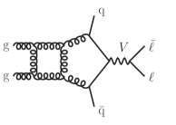
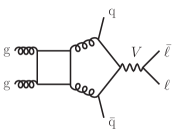
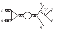
Figure 2: Sample diagrams for the different contributions to eq. 6 for $\kappa=\mathrm{g}$.

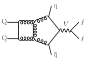
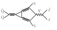
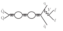
Figure 3: Sample diagrams for the different contributions to eq. 6 for $\kappa=\mathrm{Q}$.

The renormalization of the amplitudes can be performed at the renormalization scale $\mu$ by replacing the bare coupling $\alpha^{0}_{s}$ by the renormalized coupling $\alpha_{s}(\mu)$ in the perturbative expansion of the bare amplitudes $\mathcal{M}_{\kappa}$. In the $\overline{\text{MS}}$ scheme, the bare coupling is related to its renormalized counterpart by

$$\alpha_{s}^{0}\mu_{0}^{2\epsilon}S_{\epsilon}=\alpha_{s}(\mu)\mu^{2\epsilon}\left(1-\frac{\beta_{0}}{\epsilon}\frac{\alpha_{s}(\mu)}{2\pi}+\left(\frac{\beta_{0}^{2}}{\epsilon^{2}}-\frac{\beta_{1}}{2\epsilon}\right)\left(\frac{\alpha_{s}(\mu)}{2\pi}\right)^{2}+\mathcal{O}\left(\alpha_{s}^{3}(\mu)\right)\right),$$ (7)

where $\mu_{0}$ is the dimensional regularization scale, which from now on we assume to be equal to $\mu$. We will suppress the dependence on $\mu$ from all quantities. At leading color, and after setting $T_{F}=1/2$, $C_{A}=N_{c}$ and $C_{F}=(N_{c}^{2}-1)/(2N_{c})$, the coefficients of the QCD $\beta$-function are given by

$$\beta_{0} =\frac{11C_{A}-4T_{F}{N_{f}}}{6}=\frac{11N_{c}-2{N_{f}}}{6}\,,\quad$$ (8)

$$\beta_{1} =\frac{17C_{A}^{2}-6C_{F}T_{F}{N_{f}}-10C_{A}T_{F}{N_{f}}}{6}=\frac{1}{6}\left(17N_{c}^{2}-\frac{13}{2}N_{c}{N_{f}}\right)+\mathcal{O}(N_{c}^{-1})\,.$$

At each order in perturbation theory, the renormalized partial amplitudes are given by

$$\begin{split}&\mathcal{A}_{\kappa,R}^{(0)}=\mathcal{A}^{(0)}_{\kappa},\\ &\mathcal{A}_{\kappa,R}^{(1)}=\mathcal{A}_{\kappa}^{(1)}-\frac{2\beta_{0}}{\epsilon N_{c}}\mathcal{A}^{(0)}_{\kappa}\,,\\ &\mathcal{A}_{\kappa,R}^{(2)}=\mathcal{A}^{(2)}_{\kappa}-\frac{4\beta_{0}}{\epsilon N_{c}}\mathcal{A}^{(1)}_{\kappa}+\left(\frac{4\beta_{0}^{2}}{\epsilon^{2}N_{c}^{2}}-\frac{2\beta_{1}}{\epsilon N_{c}^{2}}\right)\mathcal{A}^{(0)}_{\kappa}\,.\end{split}$$ (9)

As already stated above, our calculations are done in the HV scheme of dimensional regularization and with the definition of helicity amplitudes from ref. Abreu:2018jgq . To present our results in a form that is independent of these choices (see e.g. Broggio:2015dga ) and which is sufficient for physical applications (see e.g. Weinzierl:2011uz ), we define the finite remainders $\mathcal{R}_{\kappa}$. These are obtained by removing the infrared singularities from the renormalized amplitudes, as they are determined by the previous orders in perturbation theory and known universal factors Catani:1998bh ; Becher:2009cu ; Gardi:2009qi . The finite remainders also admit an expansion in powers of the renormalized coupling,

$$\mathcal{R}_{\kappa}=\mathcal{R}^{(0)}_{\kappa}+\frac{\alpha_{s}}{2\pi}\mathcal{R}^{(1)}_{\kappa}+\left(\frac{\alpha_{s}}{2\pi}\right)^{2}\mathcal{R}^{(2)}_{\kappa}+\mathcal{O}(\alpha_{s}^{3})\,,$$ (10)

with the $\mathcal{R}_{\kappa}^{(i)}$ defined as

$$\begin{split}\mathcal{R}^{(0)}_{\kappa}&=\mathcal{A}_{\kappa,R}^{(0)},\\ \mathcal{R}^{(1)}_{\kappa}&=\mathcal{A}_{\kappa,R}^{(1)}-\mathbf{I}_{\kappa}^{(1)}\mathcal{A}_{\kappa,R}^{(0)}~{}+\mathcal{O}(\epsilon),\\ \mathcal{R}^{(2)}_{\kappa}&=\mathcal{A}_{\kappa,R}^{(2)}-\mathbf{I}_{\kappa}^{(1)}\mathcal{A}_{\kappa,R}^{(1)}-\mathbf{I}_{\kappa}^{(2)}{\cal A}_{\kappa,R}^{(0)}~{}+\mathcal{O}(\epsilon).\end{split}$$ (11)

For the amplitudes that we compute, the operators $\mathbf{I}^{(1)}_{\kappa}$ and $\mathbf{I}^{(2)}_{\kappa}$ are diagonal in color space. For each $\kappa$, the operator $\mathbf{I}^{(1)}_{\kappa}$ is given by

$${\bf I}^{(1)}_{\mathrm{g}}(\epsilon)= -\frac{e^{\gamma_{E}\epsilon}}{\Gamma(1-\epsilon)}\left(\left(\frac{1}{\epsilon^{2}}+\frac{1}{\epsilon}\frac{\beta_{0}}{{N_{c}}}\right)\left(-s_{23}\right)^{-\epsilon}+\left(\frac{1}{\epsilon^{2}}+\frac{1}{\epsilon}\frac{\beta_{0}}{2{N_{c}}}+\frac{3}{4\epsilon}\right)\left(\left(-s_{12}\right)^{-\epsilon}+\left(-s_{34}\right)^{-\epsilon}\right)\right)\,,$$

$${\bf I}^{(1)}_{\mathrm{Q}}(\epsilon)= -\frac{e^{\gamma_{E}\epsilon}}{\Gamma(1-\epsilon)}\left(\frac{1}{\epsilon^{2}}+\frac{3}{2\epsilon}\right)\left(\left(-s_{12}\right)^{-\epsilon}+\left(-s_{34}\right)^{-\epsilon}\right)\,,$$ (12)

where $s_{ij}=(p_{i}+p_{j})^{2}$ and we take the Feynman prescription $s_{ij}\rightarrow s_{ij}+i0$ wherever relevant. The operator ${\bf I}^{(2)}_{\kappa}$ is given by

$$\begin{split}{\bf I}^{(2)}_{\kappa}(\epsilon)=&-\frac{1}{2}{\bf I}^{(1)}_{\kappa}(\epsilon){\bf I}^{(1)}_{\kappa}(\epsilon)-\frac{2\beta_{0}}{{N_{c}}\epsilon}{\bf I}^{(1)}_{\kappa}(\epsilon)+\frac{e^{-\gamma_{E}\epsilon}\Gamma(1-2\epsilon)}{\Gamma(1-\epsilon)}\left(\frac{2\beta_{0}}{{N_{c}}\epsilon}+K\right){\bf I}^{(1)}_{\kappa}(2\epsilon)\\ &+\frac{e^{\gamma_{E}\epsilon}}{\epsilon\Gamma(1-\epsilon)}{\bf H}_{\kappa}\,,\end{split}$$ (13)

where

$$K=\frac{67}{9}-\frac{\pi^{2}}{3}-\frac{10}{9}\frac{{N_{f}}}{{N_{c}}}\,.$$ (14)

The operator ${\bf H}_{\kappa}$ only depends on the number of external gluons and quarks:

$${\bf H}_{\mathrm{g}}=2H_{\mathrm{g}}+2H_{\mathrm{Q}}\,,\qquad{\bf H}_{\mathrm{Q}}=4H_{\mathrm{Q}}\,,$$ (15)

with

$$\begin{split}H_{\mathrm{g}}&=\left(\frac{\zeta_{3}}{2}+\frac{5}{12}+\frac{11\pi^{2}}{144}\right)-\left(\frac{\pi^{2}}{72}+\frac{89}{108}\right)\frac{N_{f}}{{N_{c}}}+\frac{5}{27}\left(\frac{N_{f}}{{N_{c}}}\right)^{2}\,,\\ H_{\mathrm{Q}}&=\left(\frac{7\zeta_{3}}{4}+\frac{409}{864}-\frac{11\pi^{2}}{96}\right)+\left(\frac{\pi^{2}}{48}-\frac{25}{216}\right)\frac{N_{f}}{{N_{c}}}\,.\end{split}$$ (16)

We note that the definition of remainders in eq. 11 also subtracts contributions from the $\epsilon^{0}$ terms of the Laurent expansion of $\mathcal{A}_{\kappa,R}^{(1)}$ and $\mathcal{A}_{\kappa,R}^{(2)}$. The finite remainders can be expanded in powers of ${N_{f}}/{N_{c}}$, in a similar way to what was done for the partial amplitudes in eq. 6,

$$\mathcal{R}^{(k)}_{\kappa}=\sum_{j=0}^{k}\left(\frac{N_{f}}{N_{c}}\right)^{j}\mathcal{R}^{(k)[j]}_{\kappa}\,.$$ (17)

2.1 Planar Amplitudes for Four Partons and a $Z/\gamma^{*}$ Boson

In eq. 2 we used the amplitudes in LABEL:eq:partProcesses as building blocks to assemble the leading-color amplitudes for four partons and $W$ boson decaying into a lepton pair. The same building blocks can be used to compute the planar contributions for similar processes involving $Z/\gamma^{*}$ bosons decaying into a lepton pair. As in eq. 2, this is achieved by combining the amplitudes of LABEL:eq:partProcesses and dressing them with the corresponding couplings. The main difference with the $W$-boson case is that in the $Z/\gamma^{*}$ case the leading-color contributions also contain non-planar diagrams, as for example the one shown in fig. 4. Nevertheless, the planar contributions that can be obtained from LABEL:eq:partProcesses form a well-defined gauge-invariant subset of the leading-color contributions, because the missing terms can be associated to a distinct coupling structure.

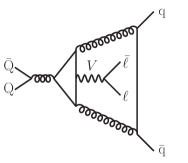
Figure 4: A non-planar diagram that contributes in the leading-color approximation to $Z$-boson production. This type of contribution has a distinct coupling structure and is consistently dropped.

Let us first consider the $Z/\gamma^{*}$ bosons decaying into a charged lepton pair. The corresponding amplitudes are given by

$$\begin{split}\mathcal{M}^{Z/\gamma^{*}}(\bar{u}_{p_{1}}^{-h},&g_{p_{2}}^{h_{2}},g_{p_{3}}^{h_{3}},u_{p_{4}}^{h},\bar{e}^{-h^{\prime}}_{p_{5}},e^{h^{\prime}}_{p_{6}})=\\ &=e^{2}\big{(}-Q_{q}+v_{e}^{h^{\prime}}v_{q}^{h}{\cal P}_{Z}(s_{56})\big{)}\mathcal{M}_{\mathrm{g}}\left(\bar{q}^{-h}_{p_{1}},g_{p_{2}}^{h_{2}},g_{p_{3}}^{h_{3}},{q}^{h}_{p_{4}};\bar{\ell}^{-h^{\prime}}_{p_{5}},{\ell}^{h^{\prime}}_{p_{6}}\right)\,,\end{split}$$ (18)

and

$$\begin{split}\mathcal{M}^{Z/\gamma^{*}}(\bar{u}_{p_{1}}^{-h},&d_{p_{2}}^{\tilde{h}},\bar{d}_{p_{3}}^{-\tilde{h}},u_{p_{4}}^{h},\bar{e}_{p_{5}}^{-h^{\prime}},e_{p_{6}}^{h^{\prime}})=\\ &=e^{2}\big{(}-Q_{u}+v_{e}^{h^{\prime}}v_{u}^{h}{\cal P}_{Z}(s_{56})\big{)}\mathcal{M}_{\mathrm{Q}}\left(\bar{q}^{-h}_{p_{1}},Q_{p_{2}}^{\tilde{h}},\bar{Q}_{p_{3}}^{-\tilde{h}},{q}^{h}_{p_{4}};\bar{\ell}^{-h^{\prime}}_{p_{5}},{\ell}^{h^{\prime}}_{p_{6}}\right)\\ &\quad+e^{2}\big{(}-Q_{d}+v_{e}^{h^{\prime}}v_{d}^{\tilde{h}}{\cal P}_{Z}(s_{56})\big{)}\mathcal{M}_{\mathrm{Q}}\left(\bar{q}^{-\tilde{h}}_{p_{3}},Q_{p_{4}}^{h},\bar{Q}_{p_{1}}^{-h},{q}^{\tilde{h}}_{p_{2}};\bar{\ell}^{-h^{\prime}}_{p_{5}},{\ell}^{h^{\prime}}_{p_{6}}\right)\,,\end{split}$$ (19)

where

$$\begin{split}\mathcal{P}_{Z}(s)&=\frac{s}{s-M_{Z}^{2}+\,\mathrm{i}\,\Gamma_{Z}M_{Z}}\,,\\ v_{e}^{-}&=v_{e}^{L}=\frac{-1+2\sin^{2}\theta_{w}}{\sin{2\theta_{w}}}\,,\quad v_{e}^{+}=v_{e}^{R}=\frac{2\sin^{2}\theta_{w}}{\sin{2\theta_{w}}}\,,\\ v_{u,d}^{-}&=v_{u,d}^{L}=\frac{\pm 1-2Q_{u,d}\sin^{2}{\theta_{w}}}{\sin{2\theta_{w}}}\,,\quad v_{u,d}^{+}=v_{u,d}^{R}=\frac{-2Q_{u,d}\sin^{2}{\theta_{w}}}{\sin{2\theta_{w}}}\,.\end{split}$$ (20)

The $Q_{u,d}$ are respectively the charges of the up-/down-type quarks, $Q_{u}=2/3$ and $Q_{d}=-1/3$. The lepton pair that couples to the photon with charge $-1$ in units of $e$ is visible in the expression $-Q_{u/d}$. In $v_{u,d}^{h}$ the upper sign corresponds to the up-type coupling $v_{u}^{h}$ and the lower one to the down-type coupling $v_{d}^{h}$.

The $Z$ boson can also decay into a pair of neutrinos. In this case, we have

$$\begin{split}\mathcal{M}^{Z}(\bar{u}_{p_{1}}^{-h},&g_{p_{2}}^{h_{2}},g_{p_{3}}^{h_{3}},u_{p_{4}}^{h},\bar{\nu}^{R}_{p_{5}},\nu^{L}_{p_{6}})=\\ &=e^{2}v_{\nu}v_{q}^{h}{\cal P}_{Z}(s_{56})\,\mathcal{M}_{\mathrm{g}}\left(\bar{q}^{-h}_{p_{1}},g_{p_{2}}^{h_{2}},g_{p_{3}}^{h_{3}},{q}^{h}_{p_{4}};\bar{\ell}^{+}_{p_{5}},{\ell}^{-}_{p_{6}}\right)\,,\\ \end{split}$$ (21)

and

$$\begin{split}\mathcal{M}^{Z}(\bar{u}_{p_{1}}^{-h},&d_{p_{2}}^{\tilde{h}},\bar{d}_{p_{3}}^{-\tilde{h}},u_{p_{4}}^{h},\bar{\nu}_{p_{5}}^{R},\nu_{p_{6}}^{L})=\\ &=e^{2}v_{\nu}v_{u}^{h}{\cal P}_{Z}(s_{56})\,\mathcal{M}_{\mathrm{Q}}\left(\bar{q}^{-h}_{p_{1}},Q_{p_{2}}^{\tilde{h}},\bar{Q}_{p_{3}}^{-\tilde{h}},{q}^{h}_{p_{4}};\bar{\ell}^{+}_{p_{5}},{\ell}^{-}_{p_{6}}\right)\\ &\quad+e^{2}v_{\nu}v_{d}^{\tilde{h}}{\cal P}_{Z}(s_{56})\,\mathcal{M}_{\mathrm{Q}}\left(\bar{q}^{-\tilde{h}}_{p_{3}},Q_{p_{4}}^{h},\bar{Q}_{p_{1}}^{-h},{q}^{\tilde{h}}_{p_{2}};\bar{\ell}^{+}_{p_{5}},{\ell}^{-}_{p_{6}}\right)\,,\end{split}$$ (22)

where

$$\begin{split}v_{\nu}&=\frac{1}{\sin{2\theta_{w}}}\,.\end{split}$$ (23)

3 Numerical Calculation of Amplitudes

Our strategy for the computation of the loop amplitudes is to reconstruct the analytic expressions from numerical samples. To simplify this process, we directly reconstruct the finite remainders defined in eq. 11, that target the new contributions at each loop order. This is achieved by first numerically reducing the amplitude to a basis of master integrals, which are themselves expanded in terms of a basis of pentagon functions Chicherin:2021dyp . We can then subtract the known divergences and obtain a numerical decomposition of the remainders in terms of pentagon functions.

Before reviewing our strategy for the numerical computation of the amplitudes and remainders, however, we start with a comment on the kinematics of the processes described by the amplitudes in LABEL:eq:partProcesses. These processes depend on six massless momenta, $p_{1}$ through $p_{6}$. However, the amplitudes can be factorized into two contributions: the first describes the scattering of four partons and a (off-shell) vector boson, and the second describes the decay of the vector boson into a pair of leptons. This is apparent in the diagrams of figs. 1, 2 and 3. While $\mathcal{M}_{\kappa}$ depends on six massless momenta, it is clear that the inherently two-loop parts of our calculation, the amplitudes for one vector boson and four partons, only depend on five momenta $p_{1}$, $p_{2}$, $p_{3}$, $p_{4}$ and $p_{\textrm{v}}=p_{5}+p_{6}$, with $p_{\textrm{v}}^{2}\neq 0$. Even though this leads to a simplification compared to genuine six-point kinematics, we note that it is nevertheless a significant increase in complexity compared to previous calculations done with the two-loop numerical unitarity approach. Indeed, only five-point massless processes have so far been computed with it, and while the algorithm itself is unaffected, some of the ingredients required at different stages had to be updated. We will highlight these updates in the following brief outline of our approach.

3.1 Two-Loop Numerical Unitarity

In order to perform the numerical reduction of the amplitudes to master integrals we use the framework of two-loop numerical unitarity Ita:2015tya ; Abreu:2017xsl ; Abreu:2017hqn ; Abreu:2018zmy ; Abreu:2018jgq ; Abreu:2020xvt . We begin by parametrizing the integrand of the partial amplitudes ${\mathcal{A}}^{(2)[j]}_{\kappa}(\ell_{l})$ in terms of master integrands, which integrate to master integrals, and surface terms, which integrate to zero Ita:2015tya . Here $\ell_{l}$ collectively denotes the loop momenta of the problem. Such a parametrization is most useful when organized in terms of propagator structures. That is, in the numerical unitarity approach we write

$${\mathcal{A}}^{(2)[j]}_{\kappa}(\ell_{l})=\sum_{\Gamma\in\Delta}\sum_{i\in M_{\Gamma}\cup S_{\Gamma}}c_{\Gamma,i}\frac{m_{\Gamma,i}(\ell_{l})}{\prod_{j\in P_{\Gamma}}\rho_{j}}\,,$$ (24)

where $\Delta$ is the set of propagator structures $\Gamma$, and $P_{\Gamma}$ is the multiset of inverse propagators $\rho_{j}$ in $\Gamma$. $M_{\Gamma}$ and $S_{\Gamma}$ denote the sets of master integrands and surface terms $m_{\Gamma,i}(\ell_{l})$ mentioned previously, and $c_{\Gamma,i}$ are the corresponding coefficients. We construct a new set of surface terms from unitarity-compatible IBP identities Ita:2015tya ; Gluza:2010ws ; Schabinger:2011dz ; Larsen:2015ped , following an approach similar to the one employed in ref. Abreu:2017hqn , the details will be presented elsewhere maxThesis . We choose the set $M_{\Gamma}$ to correspond to pure master integrals from ref. Abreu:2020jxa , which we cast into a form compatible with eq. 24 employing FiniteFlow Peraro:2019svx . In order to handle the significant increase of complexity of the sets $M_{\Gamma}$ and $S_{\Gamma}$, compared to the previously considered case of five-point massless kinematics, the implementation of the decomposition (24) within Caravel was improved. This is the first time that the decomposition in eq. 24 is obtained for processes that depend on five-point one-mass kinematics.

In order to determine the coefficients $c_{\Gamma,i}$ we rely on the factorization properties of the integrand. Specifically, we consider ${\mathcal{A}}_{\kappa}^{(2)[j]}(\ell_{l})$ on loop-momentum configurations $\ell_{l}^{\Gamma}$ where the propagators are on-shell, that is $\rho_{j}(\ell_{l}^{\Gamma})=0$ iff $j\in P_{\Gamma}$. Taking such a limit, the leading contribution to eq. (24) behaves as

$$\sum_{\text{states}}\prod_{i\in T_{\Gamma}}{\mathcal{A}}_{i}^{(0)}(\ell_{l}^{\Gamma})=\sum_{\Gamma^{\prime}\geq\Gamma,i\in M_{\Gamma^{\prime}}\cup S_{\Gamma^{\prime}}}\frac{c_{\Gamma^{\prime},i}m_{\Gamma^{\prime},i}(\ell_{l}^{\Gamma})}{\prod_{j\in(P_{\Gamma^{\prime}}\setminus P_{\Gamma})}\rho_{j}(\ell_{l}^{\Gamma})}\ .$$ (25)

On the left-hand side of this equation, we denote by $T_{\Gamma}$ the set of tree amplitudes associated with the vertices in the diagram corresponding to $\Gamma$, and the sum is over the (scheme-dependent) physical states propagating through the internal lines of $\Gamma$. On the right-hand side, we sum over the propagator structures which contribute to the limit, denoted $\Gamma^{\prime}$, for which $P_{\Gamma}\subseteq P_{\Gamma^{\prime}}$.

The coefficients $c_{\Gamma,i}$ can be determined numerically by sampling eq. 25 over a sufficient number of values of $\ell_{l}^{\Gamma}$. In order to work with color-stripped products of tree amplitudes in eq. 25 we make use of the unitarity-based color decomposition approach of refs. Ochirov:2016ewn ; Ochirov:2019mtf . In order to handle the scheme dependence inherent to the sum over states, which introduces a dependence on the dimensional regulator on the left-hand side of eq. 25, we make use of the so-called “decomposition by particle content” approach  Anger:2018ove ; Abreu:2019odu ; Sotnikov:2019onv , based on dimensional reduction. We evaluate the tree amplitudes through Berends-Giele recursion Berends:1987me . In this way, we build a constraining system of equations for the $c_{\Gamma,i}$. By performing all these calculations using finite-field arithmetic we are able to determine the coefficients exactly with no loss of precision. An important ingredient for this is a rational parametrization of phase space, that can be obtained using the momentum-twistor parametrization of ref. Hodges:2009hk . Having determined the $c_{\Gamma,i}$, we naturally arrive at the decomposition of the amplitude in terms of master integrals,

$${\mathcal{A}}^{(2)[j]}_{\kappa}=\sum_{\Gamma\in\Delta}\sum_{i\in M_{\Gamma}}c_{\Gamma,i}\mathcal{I}_{\Gamma,i}\,,$$ (26)

where $\mathcal{I}_{\Gamma,i}$ is the master integral associated with the set of propagators $\Gamma$ and numerator $m_{\Gamma,i}(\ell_{l})$. The set of master integrals relevant for this process are the planar two-loop five-point one-mass integrals, for which we use the basis of ref. Abreu:2020jxa .

3.2 Remainders and Pentagon Functions

Our goal is not to stop at the decomposition of eq. 26, that is at the decomposition of the amplitude in terms of master integrals. Rather, we want to numerically evaluate the finite remainders of eq. 11. Since the definition of the remainders involves different loop orders and the operators $\mathbf{I}_{\kappa}^{(i)}$, it cannot be decomposed into a set of master integrals. Instead, we consider all sets of master integrals that appear in the definition of the finite remainders and expand them order by order in the dimensional regulator $\epsilon$. In such an expansion, the master integrals can be expressed in terms of multiple polylogarithms (MPLs). MPLs are a class of special functions which generalize the well-known logarithm and dilogarithm and, crucially, it is nowadays well understood how to characterize all relations between them Goncharov:2010jf ; Duhr:2011zq ; Duhr:2012fh . Therefore, it is possible to construct a basis of the functions which arise in the master integrals order by order in $\epsilon$. Functions in this basis are dubbed “pentagon functions”. Such an analysis was made in ref. Chicherin:2021dyp , alongside an efficient numerical implementation of the pentagon functions, and we make use of this basis in our work.

Having evaluated the coefficients $c_{\Gamma,i}$ as described above, it is a simple algebraic procedure to discard those associated to the surface terms and insert expressions for the master integrals in terms of pentagon functions. We thereby obtain a decomposition of the amplitude in terms of pentagon functions. Denoting the relevant set of pentagon function monomials by $\{h_{i}\}_{i\in B}$, with $B$ the associated set of labels, we can then write the amplitude as

$${\mathcal{A}}^{(2)[j]}_{\kappa}=\sum_{i\in B}\sum_{k=-4}^{0}\epsilon^{k}d_{k,i}h_{i}+\mathcal{O}(\epsilon)\,,$$ (27)

where we make explicit that poles of order at most $\epsilon^{-4}$ can be found in two-loop amplitudes (we suppress the indices $\kappa$ and $j$ on the right-hand side to avoid overloading the notation). As alluded to previously, by using the decomposition in eq. 27 and its one-loop equivalent, we are able to write the one- and two-loop amplitudes in a common basis of functions. Therefore, given eqs. 11 and 17, the remainders can also be decomposed in terms of pentagon functions. That is, we write

$$\mathcal{R}^{(2)[j]}_{\kappa}=\sum_{i\in B}r_{i}h_{i}\,,$$ (28)

where the $r_{i}$ are rational functions of the external kinematics (in which we suppress for notational convenience the indices $\kappa$ and $j$). In summary, we use the two-loop numerical unitarity approach to compute the $r_{i}$ defined in eq. 28 on a given phase-space point. If desired, by using a rational parametrization of phase space, this calculation can be done over finite fields.

4 Analytic Reconstruction Algorithm

As already discussed in the previous section, although we consider six-point massless amplitudes, these are considerably simplified by the way that the vector boson couples to the rest of the process. Nevertheless, the underlying five-point one-mass kinematics makes this calculation considerably more complicated than the five-point massless amplitudes that have recently been the target of intense study. In this section we discuss a reconstruction strategy which is able to make use of the fact that the underlying kinematics of the corrections we are computing are simpler than generic six-point massless kinematics, and at the same time to handle the complex rational functions which arise. Our strategy will combine a number of ideas proposed in the literature. First, in ref. Abreu:2018zmy it was observed that the denominators of rational functions can be systematically extracted from knowledge of the coefficients on a univariate slice and the symbol alphabet. Second, in ref. Badger:2021nhg it was noticed that a univariate partial fractioning of the coefficients simplifies their analytic form in a way that is compatible with functional reconstruction approaches. Third, in ref. Klappert:2019emp , a simple method of efficiently reconstructing polynomial functions was presented where a judicious choice of sample points results in a structured linear system which can be efficiently solved. Finally, it has by now become standard to exploit the simplifications taking place when working at the level of the remainder, and so we take this as the object of final interest in our discussion.

4.1 Reduction to Five-Point One-Mass Kinematics

The amplitudes under consideration in this work depend on the kinematics of six massless particles. Since we will obtain analytic expressions with a functional reconstruction strategy, for efficiency reasons it is crucial to work with the fewest possible variables. In the following, we discuss how we reduce the six-point kinematics to an underlying set of five-point one-mass kinematics. As the discussion holds for all amplitudes $\mathcal{A}^{(i)[j]}_{\kappa}$ of eq. 6, for the purpose of readability we shall suppress indices which distinguish the various amplitudes. We begin by noting that the amplitudes $\mathcal{A}$ factorize into a QCD current $A^{\mu}$ and a tree-level leptonic current $J^{\mu}$, that is

$$\mathcal{A}=A^{\mu}J_{\mu},\quad\mathrm{where}\quad J_{\mu}=\overline{u}(p_{6})\gamma_{\mu}v(p_{5}).$$ (29)

$\overline{u}$ and $v$ are Dirac spinors of definite helicity associated to the leptons $\bar{\ell}$ and $\ell$ in fig. 1, and $A^{\mu}$ depends only on $p_{5}$ and $p_{6}$ through the combination $p_{\textrm{v}}=p_{5}+p_{6}$. The QCD current $A^{\mu}$ is a Lorentz vector and we need to specify a basis in which to express its components. As we work in the HV scheme, the contraction in equation (29) is four dimensional (see e.g. Gnendiger:2017pys ) and there are exactly four components of the vector to be determined. One of these four components can be trivially determined by noting that both $A^{\mu}$ and $J^{\mu}$ satisfy the Ward identity

$$p_{\textrm{v}}^{\mu}A_{\mu}=0,\qquad\mathrm{and}\qquad p_{\textrm{v}}^{\mu}J_{\mu}=0.$$ (30)

Therefore, only three components of $A^{\mu}$ remain to be computed in order to specify it completely. In the following, we present a strategy to reduce the calculation of these three components to that of on-shell 6-point scattering amplitudes in constrained kinematics.

We begin by considering a set of kinematic configurations where one of the leptons is collinear to one of the partons. This condition then fixes the momenta of both of the leptons via on-shellness and momentum conservation. We denote the configuration where $p_{5}$ is collinear to the momentum $p_{i}$ as

$$p_{5}^{(i)}=\frac{p_{\textrm{v}}^{2}}{2p_{i}\cdot p_{\textrm{v}}}p_{i},\ \ \ p_{6}^{(i)}=p_{\textrm{v}}-\frac{p_{\textrm{v}}^{2}}{2p_{i}\cdot p_{\textrm{v}}}p_{i}.$$ (31)

Let us stress that due to the factorization in eq. 29, the amplitude has no singularity on such configurations, spurious or otherwise. In practice, we will compute the amplitude in three such collinear configurations, specifically where $i=1,2,3$. This choice is arbitrary but we found it suitable for our reconstruction strategy to succeed. We denote the amplitude computed on these collinear configurations as $\mathcal{A}^{\{i\}}$,

$$\mathcal{A}^{\{i\}}=\mathcal{A}\left(p_{1},p_{2},p_{3},p_{4},p_{5}^{(i)},p_{6}^{(i)}\right),\qquad i=1,2,3.$$ (32)

We dub the $\mathcal{A}^{\{i\}}$ form factors, as it is possible to recover the QCD current $A^{\mu}$ from the $\mathcal{A}^{\{i\}}$. Indeed, this can be achieved by introducing a judicious partition of unity into eq. 29 as we will now make explicit. First, we introduce three reference directions defined as the leptonic current $J^{\mu}$ evaluated in each collinear configuration, that is

$$n_{i}^{\mu}=J^{\mu}\left(p_{5}^{(i)},p_{6}^{(i)}\right),\qquad i=1,2,3,$$ (33)

and we furthermore define $n_{4}^{\mu}=p_{\textrm{v}}^{\mu}$, which will allow us to directly use eq. 30 to determine one of the components of $A^{\mu}$. With these four reference directions, we decompose the four-dimensional metric tensor $g^{\mu\nu}_{(4)}$ as

$$g^{\mu\nu}_{(4)}=\sum_{i,j=1}^{4}G^{-1}_{ij}n_{i}^{\mu}n_{j}^{\nu},\qquad\mathrm{where}\qquad G_{ij}=n_{i}\cdot n_{j}.$$ (34)

Due to the Ward identity in eq. 30, $G_{i4}=G_{4j}=0$ for $i,j=1,2,3$. Employing the partition of unity (34), we can now write the QCD current $A^{\mu}$ as

$$A^{\mu}=\sum_{i,j=1}^{3}G^{-1}_{ij}\mathcal{A}^{\{i\}}n_{j}^{\mu},$$ (35)

where we have used the fact that $\mathcal{A}^{\{i\}}=A\cdot n_{i}$, for $i=1,2,3$ and eq. 30 to drop the $n_{4}$ contribution. It is therefore sufficient to compute the form factors $\mathcal{A}^{\{i\}}$, which are obtained as on-shell six-point amplitudes, in order to extract the QCD current $A^{\mu}$.

There is a technical subtlety in applying a functional reconstruction procedure to determine the $\mathcal{A}^{\{i\}}$: they are not little group invariant, and hence depend on more variables than Mandelstam invariants. This is easily remedied by factoring out some function with the same little group weights. Specifically, we make use of a standard spinor weight defined in Caravel, see Appendix A.3 of ref. Abreu:2020xvt . For the purpose of exposition, we shall suppress this in the rest of the discussion and regard $\mathcal{A}^{\{i\}}$ as a rational function of

$$\vec{s}=\{s_{\textrm{v}1},s_{12},s_{23},s_{34},s_{4\textrm{v}},p_{\textrm{v}}^{2}\}\quad\mathrm{and}\quad\mathrm{tr}_{5}=4\,\mathrm{i}\,\varepsilon_{\mu_{1}\mu_{2}\mu_{3}\mu_{4}}p_{1}^{\mu_{1}}p_{2}^{\mu_{2}}p_{3}^{\mu_{3}}p_{4}^{\mu_{4}},$$ (36)

where $s_{ij}=(p_{i}+p_{j})^{2}$, and $\varepsilon_{\mu_{1}\mu_{2}\mu_{3}\mu_{4}}$ is the fully antisymmetric Levi-Civita symbol, $\varepsilon_{0123}=1$.

To close the discussion on the reduction from six-point massless to five-point one-mass kinematics, we note that it is straightforward to define an analogue of the form factors $\mathcal{A}^{\{i\}}$ for the finite remainders. That is, we define

$$\mathcal{R}^{\{i\}}=\mathcal{R}\left(p_{1},p_{2},p_{3},p_{4},p_{5}^{(i)},p_{6}^{(i)}\right)\,,\qquad i=1,2,3,$$ (37)

implicitly considered to be normalized by the Caravel spinor weight. The $\mathcal{R}^{\{i\}}$ are sufficient to reconstruct the full finite remainders defined in eq. 11. We will target our analytic reconstruction procedure on the form-factor remainders $\mathcal{R}^{\{i\}}$, which can be decomposed in terms of pentagon functions similarly to eq. 28,

$$\mathcal{R}^{\{i\}}=\sum_{i\in B}r_{i}(\vec{s},\mathrm{tr}_{5})h_{i}\,,$$ (38)

where the $r_{i}(\vec{s},\mathrm{tr}_{5})$ are rational functions of their arguments.

4.2 Common-Denominator Form

Having reduced the problem of obtaining analytic expressions for the amplitudes in LABEL:eq:partProcesses to a functional reconstruction problem in the six variables of eq. 36, we shall now discuss the first step of our functional reconstruction strategy, which will allow us to gauge the complexity of the problem we are trying to solve.

We begin by reviewing some basic properties of the rational functions appearing in the finite remainders defined in eq. 37. As noted earlier, the amplitudes are normalized such that the functions $r_{i}$ in eq. 38 are rational functions of the Mandelstam invariants and $\mathrm{tr}_{5}$. Furthermore, as $\mathrm{tr}_{5}^{2}$ is a polynomial in the Mandelstam invariants, the dependence on it simplifies and one can write

$$r_{i}(\vec{s},\mathrm{tr}_{5})=r_{i}^{+}(\vec{s})+\mathrm{tr}_{5}\,r_{i}^{-}(\vec{s})\,,$$ (39)

where the $r_{i}^{\pm}$ are rational functions of the Mandelstam invariants. It is clear that we can evaluate the $r_{i}^{\pm}$ by computing the $r_{i}$ on parity-conjugate phase-space points Abreu:2019odu . As first suggested in ref. Abreu:2018zmy , when considered in common-denominator form the denominators of the $r_{i}^{\pm}$ factorize into products of symbol letters raised to some power. We take this form as an Ansatz and write

$$r_{i}^{\pm}=\frac{n_{i}^{\pm}}{\prod_{j=1}^{37}W_{j}^{q_{ij}^{\pm}}},$$ (40)

where the $W_{j}$ are the 37 Galois-invariant letters of the planar five-point one-mass symbol alphabet Abreu:2020jxa , and the exponents $q_{ij}^{\pm}$ are (potentially negative) integers. We note that this property holds if we normalize by the Caravel spinor-weight factor, but not necessarily if we normalize by the corresponding tree amplitudes.

To determine the exponents $q_{ij}^{\pm}$ we use the method of ref. Abreu:2018zmy . That is, we reconstruct the amplitude on a generic univariate slice of kinematic space and match the factors on the univariate slice against the symbol alphabet, performing all calculations in a finite field. In order to keep the univariate reconstruction as simple as possible, we desire a slice of phase space on which the Mandelstam behave linearly on the free parameter parametrizing the slice. In particular, this guarantees that they have the lowest possible non-trivial polynomial degree. The construction of a set of momenta corresponding to such a univariate slice is a subtle problem as it requires rationalizing $\mathrm{tr}_{5}$. Such a parametrization can be constructed on a case-by-case basis, making use of momentum-twistor parametrizations of phase space. Here we discuss an alternative and generic method of constructing a univariate slice of phase space where Mandelstam variables are linear, based on generalized BCFW shifts. Specifically, we propose to use a multi-line purely holomorphic shift Risager_2005 , as this naturally results in Mandelstam variables that are linear in the shift parameter. In order to be sufficiently generic, we shift all of the lines (see e.g. ref. Elvang:2008vz ) as proposed in ref. PageSAGEXLectures . We begin with a generic momentum configuration specified in terms of spinors $\{\lambda_{1},...,\lambda_{6},\tilde{\lambda}_{1},...,\tilde{\lambda}_{6}\}$. An all-line holomorphic shift adjusts every $\lambda$ spinor in a way which is proportional to a common reference spinor $\eta$, that is

$$\lambda_{i}\rightarrow\lambda_{i}+tc_{i}\eta.$$ (41)

Here, the $c_{i}$ are proportionality factors designed to ensure that the shifted kinematics satisfy momentum conservation, which is ensured by asking that they solve

$$\sum_{i=1}^{6}c_{i}\tilde{\lambda}_{i}=0\,.$$ (42)

This equation does not have a unique solution but any solution is suitable. Under such a shift, the holomorphic spinor products transform linearly in $t$

$$\langle ij\rangle\rightarrow\langle ij\rangle+t\,\big{(}c_{i}\langle\eta j\rangle+c_{j}\langle i\eta\rangle\big{)},$$ (43)

whereas the anti-holomorphic spinor products remain unchanged. It is therefore easy to see that the Mandelstam invariants become linear in $t$ and the pseudo-scalar $\mathrm{tr}_{5}$ is quadratic in $t$. In practice, we pick the initial set of spinor variables and the $c_{i}$ randomly over the finite field, and hence the slice we generate in this way is generic. We first generate shifted six-point kinematics, and then redefine $p_{5}$ and $p_{6}$ so that $p_{5}$ satisfies the collinearity condition specified in eq. 31.

By reconstructing the coefficients $r_{i}^{\pm}$ on a univariate slice obtained with this approach, we are able to determine the exponents $q_{ij}^{\pm}$ in eq. 40. The degree of the polynomials $n_{i}^{\pm}$ can also be determined, and in principle we could then write an Ansatz for the $n_{i}^{\pm}$ as a polynomial of that degree. For the functions we are interested in, the degree of the numerator polynomial can be sufficiently high that this Ansatz has tens of millions of free parameters. The complexity involved in solving the linear systems required to constrain such an Ansatz makes this an inviable approach to determining the analytic form of the $r_{i}^{\pm}$.

4.3 Partial-Fraction Ansatz

In order to address the problem identified above and identify simpler polynomials to reconstruct from numerical data, we employ a univariate partial-fraction decomposition as suggested in ref. Badger:2021nhg . In the following, we review this approach in order to discuss the details of our implementation.

We choose to partial fraction with respect to the Mandelstam variable $s_{34}$. This choice is made arbitrarily and it would be interesting to systematically investigate the effects of choosing other variables. To facilitate the discussion, we introduce a vector of the remaining variables, that is we define

$$\vec{s}_{\mathrm{rem}}=\left\{s_{\textrm{v}1},s_{12},s_{23},s_{4\textrm{v}},p_{\textrm{v}}^{2}\right\}.$$ (44)

We begin by reviewing the systematics of univariate partial fractioning. We start with the common-denominator representation of the rational function eq. 40, in which we recall the denominator is known fully analytically, and consider the situation where the denominator contains two factors, $W_{j_{1}}^{Q_{j_{1}}}$ and $W_{j_{2}}^{Q_{j_{2}}}$, where both $W_{j}$ are non-constant functions of $s_{34}$. We are able to break the denominator into two pieces using a solution to the equation

$$1=c_{j_{1}}(\vec{s}_{\mathrm{rem}},s_{34})W_{j_{1}}^{Q_{j_{1}}}+c_{j_{2}}(\vec{s}_{\mathrm{rem}},s_{34})W_{j_{2}}^{Q_{j_{2}}},$$ (45)

where the $c_{j}$ are polynomial in $s_{34}$ and rational in the $\vec{s}_{\mathrm{rem}}$. The existence of such solutions to eq. 45 is guaranteed by Hilbert’s Nullstellensatz as $W_{j_{1}}$ and $W_{j_{2}}$ are distinct irreducible polynomials in $s_{34}$. Equation (45) provides a decomposition of unity that we can use to break a term with multiple $s_{34}$-dependent denominators into two terms, where each term has fewer such denominators. Having started from eq. 40, we can repeatedly apply eq. 45 in order to arrive at a representation where each term has only a single denominator which depends on $s_{34}$. Once this has been achieved, to finally reach a canonical partial-fraction decomposition, the second necessary step is to cancel numerators against the denominators in $s_{34}$. This is easily achieved by polynomial division. In general this procedure will generate spurious poles, which are polynomials in $\vec{s}_{\mathrm{rem}}$ and come in two classes. The first come from the polynomial division step and are the coefficients of the leading power of $s_{34}$ in the $W_{j}$. They are trivial to generate. The second come from the splitting step and are the denominators of the $c_{i}$. To generate them, we consider all possible pairs of $W_{j}$, construct the associated pairs of $(c_{j_{1}},c_{j_{2}})$, and take their denominators. We achieve this systematically by constructing the $(c_{j_{1}},c_{j_{2}})$ pairs via Groebner basis methods, where $(c_{j_{1}},c_{j_{2}})$ are recognized as the co-factors arising in the computation of the Groebner basis of $W_{j_{1}}^{Q_{j_{1}}}$ and $W_{j_{2}}^{Q_{j_{2}}}$. We finally collect all such spurious poles together with all $s_{34}$ independent Galois-invariant letters into the set $\overline{\mathcal{W}}=\{\overline{W}_{1}(\vec{s}_{\mathrm{rem}}),\ldots,\overline{W}_{|\overline{\mathcal{W}}|}(\vec{s}_{\mathrm{rem}})\}$.

We can now describe the details of our partial-fraction decomposition of the $r_{i}^{\pm}$. We parametrize our partial-fraction decomposition as

$$r_{i}^{\pm}\!=\!\sum_{j=1}^{n_{i}}\!P_{ij}^{\pm}(\vec{s}_{\mathrm{rem}})\,g_{ij}^{\pm}(\vec{s}_{\mathrm{rem}},s_{34}),\quad\!\mathrm{with}\!\quad g_{ij}^{\pm}(\vec{s}_{\mathrm{rem}},s_{34})\!=\!\frac{Q^{\pm}_{i}(\vec{s}_{\mathrm{rem}},s_{34})s_{34}^{\alpha_{ij}^{\pm}}}{W_{k_{ij}}(\vec{s}_{\mathrm{rem}},s_{34})^{\beta_{ij}^{\pm}}\prod_{l}\overline{W_{l}}(\vec{s}_{\mathrm{rem}})^{\gamma_{ijl}^{\pm}}}.$$ (46)

Here, the $P_{ij}^{\pm}$ are polynomial in $\vec{s}_{\mathrm{rem}}$, while $g_{ij}^{\pm}$ contains all of the pole structure discussed above, both physical and spurious. The functions $Q_{i}^{\pm}$ are products of the $W_{j}$ in eq. 40 which are excluded from the partial-fraction analysis. The factors to be excluded are determined experimentally by requiring that they lower the degree of the polynomials $P_{ij}^{\pm}$. It would certainly be interesting to systematize this step of the procedure. The index $l$ runs over all elements of the set $\overline{\mathcal{W}}$ defined above. The exponents $\alpha_{ij}^{\pm},\beta_{ij}^{\pm},\gamma_{ijl}^{\pm}$ are all (potentially negative) integers. Each term in the sum in eq. 46 represents a term in the partial-fraction decomposition. Therefore, other than in the excluded piece $Q_{i}^{\pm}$, only a single denominator factor $W_{k_{ij}}$ depends on $s_{34}$.

We view eq. 46 as an Ansatz that should now be constrained from numerical data. The $Q_{i}^{\pm}$, $W_{k_{ij}}$ and $\overline{W_{l}}$ are known fully analytically, and there are two types of undetermined contributions: the polynomials $P_{ij}^{\pm}$, and the exponents $\alpha_{ij}^{\pm}$, $\beta_{ij}^{\pm}$ and $\gamma_{ijl}^{\pm}$.

We first discuss how to determine the exponents $\alpha_{ij}^{\pm}$, $\beta_{ij}^{\pm}$ and $\gamma_{ijl}^{\pm}$, as well as the total degrees of the polynomials $P_{ij}^{\pm}$. This can be achieved in a very similar way to how the exponents in the common denominator form of eq. 40 were determined. Instead of a univariate slice, however, we reconstruct the amplitude on a bivariate slice of phase space – one where $s_{34}$ varies freely and the other Mandelstam variables are linear in a parameter. Specifically, we set

$$s_{34}=s,\quad s_{\textrm{v}1}=a_{1}+b_{1}t,\quad\ldots,\quad s_{4\textrm{v}}=a_{4}+b_{4}t,\quad p_{\textrm{v}}^{2}=a_{5}+b_{5}t,$$ (47)

where the $a_{i}$ and $b_{i}$ are fixed, randomly chosen elements of a finite field that define the slice. At this stage we again face the problem that Mandelstam invariants do not rationally parametrize the phase space. To handle this difficulty, we begin with a parametrization of phase space which rationalizes the Mandelstam variables and $\mathrm{tr}_{5}$, which we detail in appendix B. This parametrization depends on the five Mandelstam variables $\vec{s}_{\mathrm{rem}}$ and a final variable $x$. The remaining Mandelstam invariant $s_{34}$ and $\mathrm{tr}_{5}$ depend rationally on these variables. We note that the parametrization is tuned such that the five $t$-dependent Mandelstam variables are explicitly independent. It is therefore trivial to choose $\vec{s}_{\mathrm{rem}}$ with a $t$ dependence as in eq. 47. To obtain the dependence on $s$, we apply the methodology of ref. Abreu:2019odu , where a change of variables is introduced in the intermediate stages of the reconstruction procedure. That is, we sample over values of $\{t,x\}$, and reconstruct the rational functions through their dependence on $\{s(t,x),t\}=\{s_{34}(t,x),t\}$. This approach also requires the ability to find parity conjugate phase-space points, which we also detail in appendix B. By reconstructing the amplitude on such a slice, and performing a univariate partial-fraction decomposition in $s$, we can evaluate the general Ansatz of eq. 46 on the bivariate slice. One can then easily identify each term in the sum of eq. 46, as they are uniquely identified by their $s_{34}$ dependence. It is then elementary to extract the degrees of $P_{ij}^{\pm}$ as well as the exponents of the factors of the $g_{ij}^{\pm}$ with the standard univariate analysis. At the end of this procedure, we have full analytic expressions for the $g_{ij}^{\pm}$, and only the polynomials $P_{ij}^{\pm}$ remain to be determined.

4.4 Vandermonde Sampling Procedure

Having determined the total degree of the $P_{ij}^{\pm}$ of eq. 46 and given that they depend on only five variables, we observe that the $P_{ij}^{\pm}$ have considerably fewer free Ansatz parameters than the $n_{i}^{\pm}$ of eq. 40. We have thus already taken an important step in addressing the problem identified at the end of section section 4.2. In this section we describe a sampling procedure which allows for an efficient determination of the $P_{ij}^{\pm}$. Specifically, we will use the Vandermonde-based approach introduced in ref. Klappert:2019emp in the context of univariate polynomial reconstruction (see also Ellis:2007br for an application of related ideas in the context of one-loop amplitudes). In our approach, which we will now detail, the generation of the numerical data is decoupled from the determination of the $P_{ij}^{\pm}$ using that data, as is commonly the case for dense functional reconstruction algorithms (see e.g. Peraro:2016wsq ).

In order to determine the $P_{ij}^{\pm}(\vec{s}_{\mathrm{rem}})$, we must first discuss how to numerically evaluate them. This is not trivial as we only have indirect access to them through eq. 46. More explicitly, given some value $\vec{s}_{\mathrm{rem}}^{(k)}$ we cannot directly evaluate the $P_{ij}^{\pm}(\vec{s}_{\mathrm{rem}}^{(k)})$ because we only have access to the numerical value of the $r_{i}^{\pm}$ (using the algorithm outlined in section 3) and the numerical value of the $g_{ij}^{\pm}$ (using their analytic expression). We can however extract the value of the $P_{ij}^{\pm}(\vec{s}_{\mathrm{rem}}^{(k)})$ by sampling eq. 46 over enough values of $s_{34}$, that is by solving the system

$$\left(\begin{matrix}g_{i1}^{\pm}(\vec{s}_{\mathrm{rem}}^{(k)},s_{34}^{(k,1)})&\cdots&g_{in_{i}}^{\pm}(\vec{s}_{\mathrm{rem}}^{(k)},s_{34}^{(k,1)})\\ \vdots&\ddots&\vdots\\ g_{i1}^{\pm}(\vec{s}^{(k)}_{\mathrm{rem}},s_{34}^{(k,n_{i})})&\cdots&g_{in_{i}}^{\pm}(\vec{s}^{(k)}_{\mathrm{rem}},s_{34}^{(k,n_{i})})\\ \end{matrix}\right)\left(\begin{matrix}P_{i1}^{\pm}(\vec{s}_{\mathrm{rem}}^{(k)})\\ \vdots\\ P_{in_{i}}^{\pm}(\vec{s}_{\mathrm{rem}}^{(k)})\\ \end{matrix}\right)=\left(\begin{matrix}r_{i}^{\pm}(\vec{s}_{\mathrm{rem}}^{(k)},s_{34}^{(k,1)})\\ \vdots\\ r_{i}^{\pm}(\vec{s}_{\mathrm{rem}}^{(k)},s_{34}^{(k,n_{i})})\\ \end{matrix}\right),$$ (48)

where $s_{34}^{(k,i)}$ denotes the different values of $s_{34}$ that are sampled (the different values are labelled by $i$, and $k$ is used to encode the fact that these different values are associated with $\vec{s}_{\mathrm{rem}}^{(k)}$). The sampling is done in a finite field, and the number of sample points, denoted by $n_{i}$, is the number of terms in the partial-fraction decomposition Ansatz of eq. 46. In practice, this number is $\mathcal{O}(10)$. We note that because we sample over arbitrary values of $s_{34}^{(k,i)}$, it is easy to pick values such that $\mathrm{tr}_{5}^{2}$ is a perfect square. Indeed, we recall that if one chooses points at random in the finite field this will be the case 50% of the time Abreu:2020jxa ; hardy1979introduction .

Now that we have discussed how to numerically evaluate the $P_{ij}^{\pm}(\vec{s}_{\mathrm{rem}}^{(k)})$ for a given value $\vec{s}_{\mathrm{rem}}^{(k)}$, we describe how to use the numerical evaluations to determine the analytic form of the $P_{ij}^{\pm}$. In principle we could sample the polynomials on enough random values of $\vec{s}_{\mathrm{rem}}^{(k)}$, but this would lead to unstructured linear systems, requiring the use of Gaussian elimination and creating a bottleneck in the procedure. Instead, we sample them on values that guarantee that the linear system to be solved corresponds to a (generalized) Vandermonde matrix. In practice, we make use of the ideas introduced in ref. Klappert:2019emp , to which we refer for further details. Here we simply outline the main steps of the approach. We begin by considering a polynomial

$$q(\vec{s}_{\mathrm{rem}})=\sum_{\vec{\alpha}_{i}\in S}c_{\vec{\alpha}_{i}}m_{\vec{\alpha}_{i}},\quad\mathrm{where}\quad m_{\vec{\alpha}_{i}}=s_{\textrm{v}1}^{\alpha_{i,1}}s_{12}^{\alpha_{i,2}}s_{23}^{\alpha_{i,3}}s_{4\textrm{v}}^{\alpha_{i,4}}p_{\textrm{v}}^{2\alpha_{i,5}},$$ (49)

and the sum over exponent vectors $\vec{\alpha}_{i}$ runs over some finite set $S$. In the absence of further information on the polynomial, this set is taken to be the full set of exponents of a homogeneous polynomial of fixed degree (we recall that we have already determined the degree of the $P_{ij}^{\pm}$). We then introduce a so-called anchor point,

$$\vec{s}_{\mathrm{rem},(0)}=\left(s_{\textrm{v}1,(0)},s_{12,(0)},s_{23,(0)},s_{4\textrm{v},(0)},p_{\textrm{v},(0)}^{2}\right),$$ (50)

from which we define further values $\vec{s}_{\mathrm{rem}}^{(k)}$ as

$$\vec{s}_{\mathrm{rem}}^{(k)}=\left(s_{\textrm{v}1,(0)}^{k},s_{12,(0)}^{k},s_{23,(0)}^{k},s_{4\textrm{v},(0)}^{k},p_{\textrm{v},(0)}^{2k}\right).$$ (51)

That is, the $k^{\textrm{th}}$ point is computed by taking the $k^{\textrm{th}}$ power of the anchor point $\vec{s}_{\mathrm{rem},(0)}$. The importance of this strategy is that the monomials behave in a structured way. More precisely, it is not hard to see that

$$m_{\vec{\alpha}_{i}}(\vec{s}_{\mathrm{rem}}^{(k)})=\left[m_{\vec{\alpha}_{i}}(\vec{s}_{\mathrm{rem},(0)})\right]^{k}.$$ (52)

If we now evaluate the polynomial $q$ on $\vec{s}_{\mathrm{rem}}^{(k)}$ for $k=1,\ldots,|S|$, then we end up with a constraining linear system for the $c_{\vec{\alpha}_{i}}$ given by

$$\left(\begin{matrix}\left[m_{\vec{\alpha}_{1}}(\vec{s}_{\mathrm{rem},(0)})\right]^{1}&\cdots&\left[m_{\vec{\alpha}_{|S|}}(\vec{s}_{\mathrm{rem},(0)})\right]^{1}\\ \vdots&\ddots&\vdots\\ \left[m_{\vec{\alpha}_{1}}(\vec{s}_{\mathrm{rem},(0)})\right]^{|S|}&\cdots&\left[m_{\vec{\alpha}_{|S|}}(\vec{s}_{\mathrm{rem},(0)})\right]^{|S|}\\ \end{matrix}\right)\left(\begin{matrix}c_{\vec{\alpha}_{1}}\\ \ldots\\ c_{\vec{\alpha}_{|S|}}\\ \end{matrix}\right)=\left(\begin{matrix}q(\vec{s}_{\mathrm{rem}}^{(1)})\\ \ldots\\ q(\vec{s}_{\mathrm{rem}}^{(|S|)})\end{matrix}\right).$$ (53)

The matrix in eq. 53 is known as a (generalized) Vandermonde matrix. The special structure of this system allows it to be efficiently solved in $\mathcal{O}(|S|^{2})$ time and $\mathcal{O}(|S|)$ space. In practice, Vandermonde systems with a side length $|S|$ of around $10^{5}$ can be solved in just over a minute on a modern laptop computer. Discussion of an efficient algorithm for solving the Vandermonde system can be found in refs. Press2007NumericalRT ; Klappert:2019emp ; PageSAGEXLectures . We note that the Vandermonde matrix becomes singular if any of the elements of a row are identical, but we did not find this to occur in practice.

Equations (48) and (53) are the cornerstones of our reconstruction procedure. The first allows us to obtain numerical values for the polynomials $P_{ij}^{\pm}$, and the second to use these numerical values to determine the analytic form of the polynomials $P_{ij}^{\pm}$. We find this reconstruction approach to have several important benefits. First, we note that it is common that, during the reconstruction procedure, one of the $P_{ij}^{\pm}$ becomes completely constrained before the full set of $P_{ij}^{\pm}$ is known. In our approach, known polynomials can easily be removed in a procedure known as “pruning” Klappert:2019emp . This leads to a significant efficiency gain. Another advantage of our approach is that it is simple to generate a sufficient set of values $\vec{s}_{\mathrm{rem}}^{(k)}$ and $s_{34}^{(k,i)}$ required for the reconstruction of all $P_{ij}^{\pm}$, and a cluster can then be used to evaluate the associated $r_{i}^{\pm}$, which is the most expensive part of the procedure. Furthermore, the approach is agnostic to the specifics of the set $|S|$. In practice, when one has performed the calculation over the first finite field, one notices that many of the coefficients $c_{\vec{\alpha_{i}}}$ are zero. With our strategy, when further finite fields are required it is trivial to implement zero coefficient constraints by simply repeating the procedure with a reduced set $S$, leading to further efficiency gains. Finally, we remark that the result is automatically homogeneous, and no procedure of de-homogenizing and re-homogenizing is required.

5 Implementation and Results

5.1 Implementation

The numerical reduction of the amplitudes to master integrals is performed with the two-loop numerical unitarity approach, as implemented in Caravel Abreu:2020xvt . Caravel was updated with the required Feynman rules, and the surface terms required for five-point one-mass planar two-loop topologies, as discussed in section 3. Starting from the decomposition into master integrals, where we use the basis of master integrals of ref. Abreu:2020jxa , we then obtain the decomposition in terms of the pentagon functions of ref. Chicherin:2021dyp . This allows us to obtain the decomposition of the remainders of eq. 38 with numerical coefficients.

These numerical evaluations are then used to obtain analytic expressions for the coefficients $r_{i}(\vec{s},{\rm tr}_{5})$ of eq. 38 with the procedure described in section 4. In order to perform the univariate and bivariate reconstructions necessary for establishing the partial-fraction Ansatz of eq. 46, we use an in-house C++ implementations of Thiele’s algorithm and of the algorithm of ref. Peraro:2016wsq , respectively. We then use Mathematica to perform the partial fractioning of the bivariate functions with respect to $s_{34}$. To simplify the reconstruction procedure, we work with only a linearly-independent set of the rational functions present in the remainder Abreu:2018aqd ; Abreu:2019rpt . That is, we express each (form factor) remainder $\mathcal{R}^{\{i\}}$, see eq. 38, in the form

$$\mathcal{R}^{\{i\}}=\sum_{k\in K,b\in B}\tilde{r}_{k}M_{kb}h_{b},$$ (54)

where $M_{kb}$ is a matrix of rational numbers, and $K$ indexes the basis of rational functions $\tilde{r}_{k}$ of the corresponding remainder. The $\tilde{r}_{k}$ are reconstructed with the approach described in section 4.4, which allows for an efficient solution of the required linear systems since they are in Vandermonde form. This procedure was implemented in a combination of Mathematica and Rust routines. Specifically, the solution of the Vandermonde system itself was implemented in Rust and linked into the Mathematica program via LibraryLink.

To illustrate the complexity of the reconstruction procedure and the impact of the partial-fraction Ansatz over the common denominator Ansatz, we record the number of free coefficients in the two Ansätze in tables 2 and 1. In these tables we do not consider $N_{f}^{2}$, as those functions are trivial compared to the $N_{f}^{0}$ and $N_{f}^{1}$ contributions. It can clearly be seen that, for all amplitudes, the univariate partial fractioning has a large effect, reducing the dimension of the Ansatz by a factor of up to $\sim 50$. We note that even after partial fractioning there are still contributions with $\mathcal{O}(500\,\textrm{k})$ undetermined parameters, and there is a large number of linear systems with $\mathcal{O}(100\,\textrm{k})$ side length to be solved. By having them in Vandermonde form, the solutions can be obtained in $\mathcal{O}(1\,\textrm{min})$ on a laptop. Furthermore, we find that once the Ansatz has been fit, there is a further strong reduction in the size of the result as many of the coefficients turn out to be zero (see the last column of tables 2 and 1). Given this sparsity, it would be interesting to consider applying sparse algorithms such as the Ben-Or/Tiwari algorithm ben1988deterministic ; Klappert:2020aqs . The fact that so many coefficients are zero has another important consequence on the efficiency of our approach, as the set of contributing monomials is known after performing the computation in the first finite field. The Vandermonde-based procedure outlined in section 4.4 is particularly suited to make use of the smaller basis of monomials when computing in more finite fields. In practice, only two finite fields of cardinality $\mathcal{O}(2^{31})$ were required to perform the rational reconstruction.

			Max Ansatz Size		Max Non-Zero Terms
$\mathcal{R}_{\mathrm{g}}$	$p_{5}\parallel p_{i}$	—K—	Common Denominator	Partial Fractioning	Result
$++$ $N_{f}^{0}$	1	29	$660$ k	$58$ k	$9$ k
	2	32	$1100$ k	$82$ k	$14$ k
	3	32	$960$ k	$87$ k	$15$ k
$++$ $N_{f}^{1}$	1	23	$380$ k	$28$ k	$5.2$ k
	2	23	$750$ k	$54$ k	$8$ k
	3	23	$580$ k	$63$ k	$11$ k
$+-$ $N_{f}^{0}$	1	58	$5500$ k	$180$ k	$37$ k
	2	67	$7000$ k	$480$ k	$110$ k
	3	67	$5900$ k	$380$ k	$90$ k
$+-$ $N_{f}^{1}$	1	50	$4600$ k	$160$ k	$33$ k
	2	53	$5000$ k	$380$ k	$87$ k
	3	53	$4200$ k	$310$ k	$75$ k
$-+$ $N_{f}^{0}$	1	75	$12\,000$ k	$210$ k	$46$ k
	2	85	$14\,000$ k	$500$ k	$130$ k
	3	85	$24\,000$ k	$430$ k	$99$ k
$-+$ $N_{f}^{1}$	1	44	$4600$ k	$120$ k	$25$ k
	2	49	$3800$ k	$210$ k	$54$ k
	3	49	$8900$ k	$270$ k	$63$ k

Table 1: Characterizing information for remainders with $\kappa=\mathrm{g}$ at various stages of the computation. We specify the remainders by the helicity states of the gluon pair and the power of $N_{f}$ (the $N_{f}^{2}$ contributions are trivial compared to the other powers, so we do not list them). $|K|$ is the dimension of the space of rational functions of the corresponding amplitude. The maximal Ansatz size in common denominator and partial-fraction form is given, when considered over all rational functions. The last column, ‘Max Non-Zero Terms’, gives the largest number of non-zero terms in the result, again taken over the basis of rational functions. Term counts are given to two significant digits for readability.

			Max Ansatz Size		Max Non-Zero Terms
$\mathcal{R}_{\mathrm{Q}}$	$p_{5}\parallel p_{i}$	—K—	Common Denominator	Partial Fractioning	Result
$+-$ $N_{f}^{0}$	1	50	$1200$ k	$53$ k	$11$ k
	2	57	$1700$ k	$210$ k	$56$ k
	3	56	$1400$ k	$240$ k	$56$ k
$+-$ $N_{f}^{1}$	1	18	$26$ k	$13$ k	$1.5$ k
	2	20	$140$ k	$47$ k	$5.1$ k
	3	20	$140$ k	$54$ k	$8.4$ k
$-+$ $N_{f}^{0}$	1	69	$2300$ k	$64$ k	$14$ k
	2	75	$2300$ k	$230$ k	$57$ k
	3	79	$5500$ k	$220$ k	$48$ k
$-+$ $N_{f}^{1}$	1	30	$240$ k	$21$ k	$3.9$ k
	2	31	$380$ k	$52$ k	$11$ k
	3	31	$380$ k	$51$ k	$9.1$ k

Table 2: Characterizing information for remainders with $\kappa=\mathrm{Q}$ at various stages of the computation. We specify the remainders by the helicity states of the quark pair not coupled to the vector boson, and the power of $N_{f}$ (the $N_{f}^{2}$ contributions are trivial compared to the other powers, so we do not list them). Column headings are identical to table 1. Term counts are given to two significant digits for readability.

5.2 Results and Validation

The main result of this paper are the analytic expressions for the two-loop remainders $\mathcal{R}_{\kappa}^{(2)[j]}$. They are given in a set of ancillary files that can be obtained from W4partonsite . Using the definition of the remainders in eq. 11, we can also assemble the two-loop amplitudes $\mathcal{A}^{(2)[j]}$. This requires the knowledge of the one-loop amplitudes $\mathcal{A}^{(1)[j]}$, and we have thus also recomputed them using similar reconstruction techniques. In fact, the one-loop amplitudes are presented as a decomposition in terms of master integrals, that is we reconstruct the coefficients $c_{\Gamma,i}$ in the one-loop equivalent of the decomposition of eq. 26, where for the basis of master integrals we take the one-loop basis used in Abreu:2020jxa . We also include a map from the one-loop integrals to the pentagon functions of ref. Chicherin:2021dyp up to weight 4, so that the one-loop expressions can be written as a decomposition in terms of pentagon functions similar to the format we use for the two-loop remainders. Provided the one-loop integrals are known, the expressions we present for the one-loop amplitudes can however be used to expand the amplitudes to arbitrary order in $\epsilon$, extending the results of refs. Bern:1997sc ; Bern:1996ka . All the components required to assemble the one-loop amplitudes are also in the set of ancillary files.

To facilitate the use of our ancillary files, we include a Mathematica script called amp_eval.m which assembles the different components required to evaluate the one-loop and two-loop amplitudes and remainders, and evaluates them at the phase-space point specified in appendix C. The target values obtained by running this script are also included in appendix C, see tables 3, 4 and 5. Together with the README.md file, the script was prepared to document the different files and be a good entry point to start exploring our results.

Let us briefly comment on the analytic structure of the two-loop amplitudes we computed. It was observed in ref. Badger:2021nhg that the pentagon functions involving the letters $\{W_{16},W_{17},W_{27},W_{28},W_{29},W_{30}\}$ (we use the notation of ref. Abreu:2020jxa ), which are present in the contributing master integrals, drop out from the squared amplitudes for on-shell $Wb\overline{b}$ production when expanded to finite order in $\epsilon$. The same observation was made in ref. Badger:2021ega for the two-loop finite remainders for the production of a $H$ boson in association with a $b\bar{b}$ pair. We observe here that the same holds also at the level of helicity form factors for both the quark and gluon partonic processes considered in this work. Furthermore, we also observe that the pentagon functions involving the letter $\mathrm{tr}_{5}$ do not appear in the finite remainders, an interesting fact that has been previously linked to cluster algebras Chicherin:2020umh . We note that the pentagon-function basis of ref. Chicherin:2021dyp has been constructed in a way that such cancellations are manifest.

We have performed a number of checks, not only on our final results, but also on the intermediate steps of our calculation. Let us first discuss the internal checks performed on the intermediate stages of the calculation. Since this is the first time we have used the surface terms for five-point one-mass kinematics (see the discussion in section 3.1), we have numerically cross-checked them against FIRE Smirnov:2008iw ; Smirnov:2014hma . The numerical evaluation of the amplitudes was performed within the numerical-unitarity code Caravel Abreu:2020xvt , which includes many internal self-consistency checks. The numerical calculation of the two-loop remainders is also performed within Caravel, and at each phase-space point we thus verify that the amplitude has the pole structure predicted by eq. 11. After obtaining the analytic expression for the one-loop amplitudes and the two-loop remainders, we performed consistency checks to verify that the reconstructed expressions agree with the numerical evaluations obtained with Caravel. Finally, we verified that the reconstructed expressions, which are obtained from numerical evaluations in a finite field, agree with floating-point numerical evaluations within Caravel.

Let us now discuss the checks we have made on the final results we have obtained. First, the one-loop amplitudes were checked up to order $\epsilon^{0}$ with the results obtained from the BlackHat library Berger:2008sj . Second, we reproduced the numerical table of ref. Hartanto:2019uvl using Caravel to evaluate the master integral coefficients and DiffExp Hidding:2020ytt to evaluate the master integrals. This is a strong check of the correctness of the numerical evaluations within Caravel, which we used to obtain our analytic expressions. Third, we reproduced the results of ref. Badger:2021nhg for unpolarized on-shell $Wb\overline{b}$ production by squaring our currents $A^{\mu}$ in eq. 29 appropriately. This is a particularly stringent test, as the calculation in ref. Badger:2021nhg is performed in the conventional dimensional regularization (CDR) scheme, and using the Larin’s $\gamma_{5}$ prescription Larin:1993tq . The latter produces non-trivial differences between vector and axial currents, and we find agreement at the level of the finite remainders.

Finally, let us mention that given our analytic results in the form of eq. 54, which are valid for the partonic channels of LABEL:eq:partProcesses with momenta $p_{1}$ and $p_{2}$ incoming, it is straightforward to obtain results in other partonic channels by permutations of particles’ momenta. Indeed, the action of permutations on the rational functions $\tilde{r}_{i}(\vec{s},\mathrm{tr}_{5})$ is obvious. The action of permutations on the one-mass pentagon functions $h_{i}$ is discussed in section 3.2 of ref. Chicherin:2021dyp , and is explicitly provided in the supplementary materials thereof. It is worth noting that the latter allows us to replace the dedicated analytic continuation procedure which had to be employed, for instance, in ref. Abreu:2021oya , by simple substitutions.

6 Conclusions and Outlook

We have computed the analytic expressions for the planar two-loop QCD corrections to the helicity amplitudes for four partons and a vector boson that decays into a lepton pair. These expressions allow us to compute the full leading color two-loop QCD corrections to amplitudes for four partons and a $W$ boson that decays into a lepton pair. Furthermore, they also fully determine the gauge-invariant planar contributions to the same amplitudes where the $W$ boson is replaced by a $Z/\gamma^{*}$ (in this case, some leading-color corrections have non-planar contributions, but they can be separated from the contributions we compute because they have a distinct coupling structure).

The analytic results we present are reconstructed from numerical evaluations, an approach that has been very successfully applied to five-point massless processes. We find that there is a marked increase in complexity when considering five-point one-mass kinematics. This led us to develop a more efficient reconstruction approach, building on a partial-fraction Ansatz Badger:2021nhg and on a judicious numerical sampling procedure that leads to linear systems in Vandermonde form. Conveniently, the numerical evaluations of the amplitudes and the reconstruction of the analytic functions remain decoupled in this approach.

We have explicitly presented the analytic expressions that are valid in the region where $p_{1}$ and $p_{2}$ are incoming. The expressions in the other regions can be straightforwardly obtained by considering appropriate combinations of particles’ momenta permutations, charge and parity conjugation. Given the analytic complexity of the derived amplitudes and the large number of required partonic channels, we leave an efficient implementation of their numerical evaluation and the study of numerical stability for future work.

Given the remarkable progress in handling the real-radiation contribution with complex final-state jet structure at NNLO QCD (see e.g. Czakon:2021mjy ), we expect that NNLO QCD predictions for the production of a $W$ boson in association with two jets at hadron colliders are now within reach.

Appendix A Axial-vector and Vector Couplings

In this section, we discuss the equivalence of vector and axial-vector currents up to a sign in massless QCD, which holds as long as the axial-vector couplings to closed fermion loops are excluded.

The diagrams contributing to the vector and axial-vector current are schematically represented in fig. 5. In four dimensions these diagrams give rise to the spinor chains

$$S^{\mu} =\bar{u}^{R}\,\cdots{}\gamma^{\mu}\cdots{}\,v^{L},$$ (55a)

$$S^{\mu}_{5} =\bar{u}^{R}\,\cdots{}\gamma^{\mu}\gamma^{5}\cdots{}\,v^{L}\,,$$ (55b)

where we use lower case $\gamma^{\prime}s$ for the four dimensional Clifford algebra and $\gamma^{5}:=\tilde{\gamma}=\,\mathrm{i}\,\gamma^{0}\gamma^{1}\gamma^{2}\gamma^{3}$ with $(\gamma^{5})^{2}=\mathbb{1}$. Without loss of generality, we consider the spinor chains with left-handed quarks and right-handed anti-quarks.

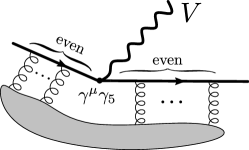
Figure 5: The structure of diagrams contributing to axial-vector currents considered in this work. The shaded blob contains the remaining external particles, as well as loops. Each gluon that couples to the quark line adds two additional $\gamma$-matrices to the spinor chain, one from the interaction vertex and one from the additional quark propagator.

We begin by confirming that in four dimensions the currents differ by sign,

$$S^{\mu}=-S^{\mu}_{5}\,.$$ (56)

Indeed, by inspecting the diagrams in fig. 5 we observe that we can always anticommute $\gamma^{5}$ through an even number of $\gamma$-matrices to the right (or odd number of $\gamma$ matrices to the left) and use the definition,

$$\gamma^{5}\,v^{L}=-v^{L}\quad\mbox{and}\quad\bar{u}^{R}(p)\,\gamma^{5}=\bar{u}^{R}(p)\,,$$ (57)

to eliminate $\gamma^{5}$ from any spinor chain.

In the following we discuss that the same relation holds in dimensional regularization within Kreimer’s anticommuting $\gamma^{5}$ scheme Kreimer:1989ke ; Korner:1991sx . In this scheme one starts with the $D$-dimensional Clifford algebra $\{\Gamma^{\mu}\}$,

$$\left\{\Gamma^{\mu},\Gamma^{\nu}\right\}=2g^{\mu\nu}\,\mathbb{1}\,,\quad\left\{\tilde{\Gamma},\Gamma^{\mu}\right\}=0\quad\mbox{and}\quad\tilde{\Gamma}^{2}=\mathbb{1}.$$ (58)

Here $\tilde{\Gamma}$ is the $D$-dimensional generalisation of $\gamma^{5}$, which allows to construct chirality projectors. We will also use the literal embedding of $\gamma^{5}$ in the D-dimensional Clifford algebra, namely

$$\Gamma^{5}=\,\mathrm{i}\,\Gamma^{0}\Gamma^{1}\Gamma^{2}\Gamma^{3}\,.$$ (59)

Any element $F$ in the $D$-dimensional Clifford algebra can be expanded into a basis

$$F=f\mathbb{1}+f_{\mu}\Gamma^{\mu}+f_{\mu_{1}\mu_{2}}\Gamma^{\mu_{1}\mu_{2}}+f_{\mu_{1}\mu_{2}\mu_{3}}\Gamma^{\mu_{1}\mu_{2}\mu_{3}}+\ldots{},$$ (60)

where the basis elements $\Gamma^{\mu_{1}\cdots{}\mu_{n}}$ are anti-symmetrized products of $n$ $\Gamma$-matrices. In Kreimer’s $\gamma^{5}$ scheme one replaces $\gamma^{\mu}\to\Gamma^{\mu},~{}\gamma^{5}\to\tilde{\Gamma}$, and the anticommutativity of $\tilde{\Gamma}$ is used to ensure that at most one $\tilde{\Gamma}$ appears in each spinor chain. The evaluation of spinor chains is formulated in terms of trace operations $\operatorname{Tr}[\cdot]$, which return particular coefficients in the decomposition of eq. 60,

$$\operatorname{Tr}[F] \coloneqq 4\,f=4\,\frac{\operatorname{tr}[F]}{\operatorname{tr}[\mathbb{1}]},$$ (61a)

$$\operatorname{Tr}[\tilde{\Gamma}F] \coloneqq 4\,f_{0123}=4\,\frac{\operatorname{tr}[\Gamma^{5}F]}{\operatorname{tr}[\mathbb{1}]}\,.$$ (61b)

Here $\operatorname{tr}[\cdot]$ is the conventional trace for $\Gamma$-matrices. With this definition, a single $\tilde{\Gamma}$, if present, is moved to the left in products of $\Gamma$-matrices. This operation is always possible in fixed-order computations based on Feynman rules. In the second line we used the orthogonality of the basis $\Gamma^{\mu_{1}…\mu_{n}}$ to obtain the coefficient $f_{0123}$ using the insertion $\Gamma^{5}$ in $\operatorname{tr}[\cdot]$ Korner:1991sx . In practice, we can work without making the $\tilde{\Gamma}$ factor manifest and obtain the convenient trace prescription,

$$F^{\prime}=\tilde{\Gamma}F\,,\quad\operatorname{Tr}[F^{\prime}]=\operatorname{Tr}[\tilde{\Gamma}^{2}F^{\prime}]=\operatorname{Tr}[\tilde{\Gamma}(\tilde{\Gamma}F^{\prime})]=4\,\frac{\operatorname{tr}[\Gamma^{5}\tilde{\Gamma}F^{\prime}]}{\operatorname{tr}[\mathbb{1}]}\,.$$ (62)

This amounts to inserting $(\Gamma^{5}\tilde{\Gamma})$ at a fixed point in the spinor chain before evaluating the conventional trace $\operatorname{tr}[\cdot]$. As we will now see, for spinor chains with external states the insertion point is naturally given.

We are now in the position to discuss the effect of the above prescription for evaluating the spinor chains $S^{\mu}$ and $S^{\mu}_{5}$. First we use the $D$-dimensional generalization of the spinor states discussed in ref. Abreu:2018jgq , which are a tensor product of four-dimensional states and a spinor basis beyond four dimensions. For simplicity we denote two such spinors by the same symbols as above $\bar{u}^{R}$ and $v^{L}$ and use $\bar{u}^{R}\Gamma^{5}=\bar{u}^{R}$ and $\Gamma^{5}v^{L}=-v^{L}$, which is a trivial consequence of eq. 59. We obtain,

$$S^{\mu} \coloneqq\bar{u}^{R}\,\cdots{}\Gamma^{\mu}\cdots{}\,v^{L},$$ (63a)

$$S^{\mu}_{5} \coloneqq\bar{u}^{R}\,\cdots{}\Gamma^{\mu}\tilde{\Gamma}\cdots{}\,v^{L}\,.$$ (63b)

We now rewrite the spinor chains in terms of the $\operatorname{Tr}[\cdot]$ operation. For the contributions including $\tilde{\Gamma}$ we have to consistently chose an insertion point for $\Gamma^{5}\tilde{\Gamma}$. A well defined choice is to insert after the $\bar{u}$ spinor associated to the external state. Using the properties in eqs. 58 and 61 we obtain

$$\begin{split}S^{\mu}_{5}&=\operatorname{Tr}[v^{L}\bar{u}^{R}\cdots{}\Gamma^{\mu}\tilde{\Gamma}\cdots{}]=\operatorname{tr}[v^{L}\bar{u}^{R}(\Gamma^{5}\tilde{\Gamma})\cdots{}\Gamma^{\mu}\tilde{\Gamma}\cdots{}]\\ &=-\operatorname{tr}[v^{L}\bar{u}^{R}\Gamma^{5}\cdots{}\Gamma^{\mu}\cdots{}]=-\operatorname{tr}[v^{L}\bar{u}^{R}\cdots{}\Gamma^{\mu}\cdots{}]\\ &=-S^{\mu}\,.\end{split}$$ (64)

where we used that $\bar{u}^{R}\Gamma^{5}=\bar{u}^{R}$ and $\{\Gamma^{\mu},\tilde{\Gamma}\}=0$. This demonstrates that $S^{\mu}=-S^{\mu}_{5}$ can be maintained in dimensional regularization.

As pointed out in refs. Kreimer:1989ke ; Korner:1991sx the trace operation $\operatorname{Tr}[\cdot]$ involving $\tilde{\Gamma}$ does not satisfy cyclicity. Generally, this implies that all traces must be consistently evaluated with reference to a point where we insert $\Gamma^{5}\tilde{\Gamma}$. Conveniently, the spinor chains in eq. 63 have a distinguished insertion point, namely next to the $\bar{u}$ spinor. This insertion point is not only unambiguous, but also aligns signs of the four-dimensional algebra and the $D$-dimensional one. Finally, let us recall that we do not consider contributions with axial couplings to closed fermion loops, therefore we are not concerned with axial anomalies in this paper.

In summary we showed the equivalence of vector and axial-vector currents for spinor chains bounded by external states. In addition we obtain a simple prescription to handle axial-vector couplings following refs. Kreimer:1989ke ; Korner:1991sx . This prescription is particularly convenient for our approach to dimensional regularization of helicity amplitudes Abreu:2018jgq , which is realized entirely in integer dimensions and therefore suitable for direct numerical implementation.

Appendix B Rationalization of $\mathrm{tr}_{5}$

In this appendix we present the explicit form of the rational parametrization of the five-point one-mass phase-space which we use in the procedure described in section 4.3 to constrain the partial-fraction Ansatz of eq. 46. To rationalize ${\rm tr}_{5}$ we use a parametrization in which only one variable is not a Mandelstam invariant. More explicitly, we use the variables

$$\{s_{\textrm{v}1},s_{12},s_{23},s_{4\textrm{v}},p_{\textrm{v}}^{2},x\},$$ (65)

where $x$ is chosen such that $s_{34}$ and $\mathrm{tr}_{5}$ are rational in the variables of eq. 65. Explicitly, they are given by

$$\begin{split}\mathrm{tr}_{5}(&s_{\textrm{v}1},s_{12},s_{23},s_{4\textrm{v}},p_{\textrm{v}}^{2},x)=\frac{s_{\textrm{v}1}(s_{4\textrm{v}}-s_{12})+(s_{12}-p_{\textrm{v}}^{2})s_{23}}{4\,\big{(}(s_{4\textrm{v}}-s_{23})^{2}-[s_{\textrm{v}1}(s_{4\textrm{v}}-s_{12})+(s_{12}-p_{\textrm{v}}^{2})s_{23}]^{2}x^{2})\big{)}}\\ &\times\Big{[}(s_{4\textrm{v}}-s_{23})^{2}+\\ &\quad\,\,2\big{(}s_{\textrm{v}1}s_{4\textrm{v}}(s_{12}\!-\!s_{4\textrm{v}})+[p_{\textrm{v}}^{2}(s_{4\textrm{v}}\!-\!2s_{12})+s_{4\textrm{v}}s_{12}+s_{\textrm{v}1}(s_{4\textrm{v}}\!+\!s_{12})]s_{23}-(p_{\textrm{v}}^{2}\!+\!s_{12})s_{23}^{2}\big{)}x\\ &\quad+(s_{\textrm{v}1}(s_{4\textrm{v}}-s_{12})+(s_{12}-p_{\textrm{v}}^{2})s_{23})^{2}x^{2}\Big{]}\,,\end{split}$$ (66)

$$\begin{split}s_{34}(&s_{\textrm{v}1},s_{12},s_{23},s_{4\textrm{v}},p_{\textrm{v}}^{2},x)=\frac{2}{(s_{\textrm{v}1}(s_{4\textrm{v}}-s_{12})+(s_{12}-p_{\textrm{v}}^{2})s_{23})^{2}x^{2}-(s_{4\textrm{v}}-s_{23})^{2}}\\ &\times\Big{[}(s_{\textrm{v}1}s_{4\textrm{v}}s_{12}-s_{\textrm{v}1}s_{4\textrm{v}}^{2}+p_{\textrm{v}}^{2}s_{4\textrm{v}}s_{23}+s_{\textrm{v}1}s_{4\textrm{v}}s_{23}-2p_{\textrm{v}}^{2}s_{12}s_{23}+s_{\textrm{v}1}s_{12}s_{23}\\ &\quad+s_{4\textrm{v}}s_{12}s_{23}-p_{\textrm{v}}^{2}s_{23}^{2}-s_{12}s_{23}^{2}+(s_{\textrm{v}1}(s_{4\textrm{v}}-s_{12})+(s_{12}-p_{\textrm{v}}^{2})s_{23})^{2}x)\Big{]}\,.\end{split}$$ (67)

In order to disentangle the $r_{i}^{+}(\vec{s})$ and $r_{i}^{-}(\vec{s})$ contributions in the coefficients $r_{i}(\vec{s},{\rm tr}_{5})$ of eq. 39, we need to identify the phase-space point that is related by parity conjugation to the point corresponding to eq. 65. Indeed, parity conjugation flips the sign of ${\rm tr}_{5}$ and leaves the Mandelstam variables invariant, and by evaluating $r_{i}(\vec{s},{\rm tr}_{5})$ in pairs of parity-conjugate points we can determine $r_{i}^{+}(\vec{s})$ and $r_{i}^{-}(\vec{s})$. The parity-conjugate point

$$\{s_{\textrm{v}1},s_{12},s_{23},s_{4\textrm{v}},p_{\textrm{v}}^{2},\bar{x}\},$$ (68)

must be such that

$$\begin{split}\mathrm{tr}_{5}(s_{\textrm{v}1},s_{12},s_{23},s_{4\textrm{v}},p_{\textrm{v}}^{2},\bar{x})=-\mathrm{tr}_{5}(s_{\textrm{v}1},s_{12},s_{23},s_{4\textrm{v}},p_{\textrm{v}}^{2},x),\\ s_{34}(s_{\textrm{v}1},s_{12},s_{23},s_{4\textrm{v}},p_{\textrm{v}}^{2},\bar{x})=s_{34}(s_{\textrm{v}1},s_{12},s_{23},s_{4\textrm{v}},p_{\textrm{v}}^{2},x).\end{split}$$ (69)

Solving for $\bar{x}$, we find

$$\begin{split}\bar{x}&=\Big{[}-(s_{4\textrm{v}}-s_{23})^{2}+(s_{\textrm{v}1}s_{4\textrm{v}}(s_{4\textrm{v}}-s_{12})-(p_{\textrm{v}}^{2}(s_{4\textrm{v}}-2s_{12})\\ &\qquad+s_{4\textrm{v}}s_{12}+s_{\textrm{v}1}(s_{4\textrm{v}}+s_{12}))s_{23}+(p_{\textrm{v}}^{2}+s_{12})s_{23}^{2})x\Big{]}/\Big{[}s_{\textrm{v}1}s_{4\textrm{v}}s_{12}\\ &\qquad-s_{\textrm{v}1}s_{4\textrm{v}}^{2}+p_{\textrm{v}}^{2}s_{4\textrm{v}}s_{23}+s_{\textrm{v}1}s_{4\textrm{v}}s_{23}-2p_{\textrm{v}}^{2}s_{12}s_{23}+s_{\textrm{v}1}s_{12}s_{23}\\ &\qquad+s_{4\textrm{v}}s_{12}s_{23}-p_{\textrm{v}}^{2}s_{23}^{2}-s_{12}s_{23}^{2}+(s_{\textrm{v}1}(s_{4\textrm{v}}-s_{12})+(-p_{\textrm{v}}^{2}+s_{12})s_{23})^{2}x\Big{]}\,.\end{split}$$ (70)

Appendix C Benchmark numerical evaluation

To facilitate comparisons with our results, we provide benchmark numerical evaluations for all the helicity amplitudes we computed. We evaluate the bare helicity amplitudes and finite remainders on a generic point from physical six-point massless phase-space, where the momenta $p_{1}$ and $p_{2}$ are incoming. The point we choose corresponds to

$$\begin{gathered}s_{12}=5,\quad s_{23}=-\frac{1}{3},\quad s_{34}=\frac{11}{13},\quad s_{456}=\frac{17}{19},\quad s_{156}=-\frac{23}{29},\quad s_{56}=\frac{1}{7},\\ s_{345}=\frac{4304788}{896077},\quad s_{45}=\frac{2911673}{3928953},\quad s_{16}=-\frac{186065}{1998941},\qquad{\rm tr}_{5}=-\frac{10\,\mathrm{i}\,\sqrt{292010395}}{150423},\end{gathered}$$ (71)

where the first line specifies the reduction to the five-point one-mass kinematics (we recall that $p_{\textrm{v}}=p_{5}+p_{6}$).

We present the amplitudes for four partons and $W^{+}(\to\bar{e}^{+}\nu^{-})$, i.e.

$$\begin{split}\mathcal{A}^{(l)[j]}_{\mathrm{g};h_{2}h_{3}}&=\mathcal{A}^{(l)[j]}(\bar{u}_{1}^{+},g_{2}^{h_{2}},g_{3}^{h_{3}},d_{4}^{-};\bar{e}^{+}_{5},\nu_{6}^{-}),\\ \mathcal{A}^{(l)[j]}_{\mathrm{Q};h_{2}h_{3}}&=\mathcal{A}^{(l)[j]}(\bar{u}_{1}^{+},Q_{2}^{h_{2}},\bar{Q}_{3}^{h_{3}},d_{4}^{-};\bar{e}_{5}^{+},\nu_{6}^{-}),\end{split}$$ (72)

where we recall that we label all particles as outgoing. The numerical results we present are normalized to the corresponding tree amplitudes to make the pole structure manifest.

$\epsilon^{-2}$ $\epsilon^{-1}$ $\epsilon^{0}$ $\epsilon^{1}$ $\epsilon^{2}$ $\mathcal{A}^{(1)[0]}_{\mathrm{g};++}$ $-3.000000000$ $-1.156228461$ $-6.283185307\,\mathrm{i}\,$ $114.1571538$ $-22.50315905\,\mathrm{i}\,$ $390.7700369$ $-27.70171948\,\mathrm{i}\,$ $772.8514956$ $-47.35817758\,\mathrm{i}\,$ $\mathcal{A}^{(1)[1]}_{\mathrm{g};++}$ $0$ $0$ $-80.09777916$ $+22.21916010\,\mathrm{i}\,$ $-381.6882614$ $+105.8804960\,\mathrm{i}\,$ $-1061.591691$ $+294.4860144\,\mathrm{i}\,$ $\mathcal{A}^{(1)[0]}_{\mathrm{g};-+}$ $-3.000000000$ $-1.156228461$ $-6.283185307\,\mathrm{i}\,$ $9.229250985$ $-11.92991811\,\mathrm{i}\,$ $21.88019567$ $-11.15992632\,\mathrm{i}\,$ $28.67469046$ $+1.329575472\,\mathrm{i}\,$ $\mathcal{A}^{(1)[1]}_{\mathrm{g};-+}$ $0$ $0$ $0$ $0$ $0$ $\mathcal{A}^{(1)[0]}_{\mathrm{g};+-}$ $-3.000000000$ $-1.156228461$ $-6.283185307\,\mathrm{i}\,$ $10.84787275$ $-11.33482230\,\mathrm{i}\,$ $28.55563117$ $-7.684296706\,\mathrm{i}\,$ $42.82153823$ $+12.66461492\,\mathrm{i}\,$ $\mathcal{A}^{(1)[1]}_{\mathrm{g};+-}$ $0$ $0$ $0$ $0$ $0$ $\mathcal{A}^{(1)[0]}_{\mathrm{Q};-+}$ $-2.000000000$ $2.109050494$ $-6.283185307\,\mathrm{i}\,$ $16.14776220$ $-12.06220529\,\mathrm{i}\,$ $33.34325904$ $-10.91964040\,\mathrm{i}\,$ $44.03129425$ $+3.915968598\,\mathrm{i}\,$ $\mathcal{A}^{(1)[1]}_{\mathrm{Q};-+}$ $0$ $-0.6666666667$ $-1.843519304$ $-3.148759359$ $-3.759742920$ $\mathcal{A}^{(1)[0]}_{\mathrm{Q};+-}$ $-2.000000000$ $2.109050494$ $-6.283185307\,\mathrm{i}\,$ $17.40843911$ $-12.56539566\,\mathrm{i}\,$ $39.85865914$ $-10.64655144\,\mathrm{i}\,$ $57.30017001$ $+11.51871433\,\mathrm{i}\,$ $\mathcal{A}^{(1)[1]}_{\mathrm{Q};+-}$ $0$ $-0.6666666667$ $-1.843519304$ $-3.148759359$ $-3.759742920$

Table 3: Bare one-loop amplitudes of eq. 72 evaluated at the phase-space point of eq. 71, normalized by the corresponding tree amplitude. The numerical results are rounded to fit the table.

$\epsilon^{-4}$ $\epsilon^{-3}$ $\epsilon^{-2}$ $\epsilon^{-1}$ $\epsilon^{0}$ $\mathcal{A}^{(2)[0]}_{\mathrm{g};++}$ $4.500000000$ $0.7186853827$ $+18.84955592\,\mathrm{i}\,$ $-366.7779225$ $+63.25510176\,\mathrm{i}\,$ $-1031.818957$ $-703.7101696\,\mathrm{i}\,$ $2229.756465$ $-4271.317939\,\mathrm{i}\,$ $\mathcal{A}^{(2)[1]}_{\mathrm{g};++}$ $0$ $0.5000000000$ $241.5120803$ $-64.56308519\,\mathrm{i}\,$ $1008.875317$ $+259.9002941\,\mathrm{i}\,$ $-311.1773011$ $+3729.331393\,\mathrm{i}\,$ $\mathcal{A}^{(2)[2]}_{\mathrm{g};++}$ $0$ $0$ $0$ $53.39851944$ $-14.81277340\,\mathrm{i}\,$ $402.1206430$ $-111.5484479\,\mathrm{i}\,$ $\mathcal{A}^{(2)[0]}_{\mathrm{g};-+}$ $4.500000000$ $0.7186853827$ $+18.84955592\,\mathrm{i}\,$ $-51.99421404$ $+31.53537893\,\mathrm{i}\,$ $-122.1308176$ $-67.51062386\,\mathrm{i}\,$ $-13.35042281$ $-373.3014208\,\mathrm{i}\,$ $\mathcal{A}^{(2)[1]}_{\mathrm{g};-+}$ $0$ $0.5000000000$ $1.218742820$ $+2.094395102\,\mathrm{i}\,$ $-4.764106945$ $+11.44393724\,\mathrm{i}\,$ $-39.16109323$ $+32.37695552\,\mathrm{i}\,$ $\mathcal{A}^{(2)[2]}_{\mathrm{g};-+}$ $0$ $0$ $0$ $0$ $0$ $\mathcal{A}^{(2)[0]}_{\mathrm{g};+-}$ $4.500000000$ $0.7186853827$ $+18.84955592\,\mathrm{i}\,$ $-56.85007933$ $+29.75009152\,\mathrm{i}\,$ $-134.3545770$ $-86.61366193\,\mathrm{i}\,$ $31.37211219$ $-446.6498136\,\mathrm{i}\,$ $\mathcal{A}^{(2)[1]}_{\mathrm{g};+-}$ $0$ $0.5000000000$ $1.218742820$ $+2.094395102\,\mathrm{i}\,$ $-5.843188121$ $+11.04720671\,\mathrm{i}\,$ $-49.02848488$ $+27.67994158\,\mathrm{i}\,$ $\mathcal{A}^{(2)[2]}_{\mathrm{g};+-}$ $0$ $0$ $0$ $0$ $0$ $\mathcal{A}^{(2)[0]}_{\mathrm{Q};-+}$ $2.000000000$ $-6.051434322$ $+12.56637061\,\mathrm{i}\,$ $-48.02138179$ $-0.6463175652\,\mathrm{i}\,$ $-45.51885333$ $-162.3399739\,\mathrm{i}\,$ $286.8120373$ $-570.6619745\,\mathrm{i}\,$ $\mathcal{A}^{(2)[1]}_{\mathrm{Q};-+}$ $0$ $1.666666667$ $0.9113214460$ $+6.283185307\,\mathrm{i}\,$ $-25.99983021$ $+31.15677229\,\mathrm{i}\,$ $-139.3729721$ $+83.16373240\,\mathrm{i}\,$ $\mathcal{A}^{(2)[2]}_{\mathrm{Q};-+}$ $0$ $0$ $0.4444444444$ $2.458025738$ $7.596909235$ $\mathcal{A}^{(2)[0]}_{\mathrm{Q};+-}$ $2.000000000$ $-6.051434322$ $+12.56637061\,\mathrm{i}\,$ $-50.54273561$ $+0.3600631747\,\mathrm{i}\,$ $-54.42997862$ $-173.7135037\,\mathrm{i}\,$ $349.9447856$ $-655.1503315\,\mathrm{i}\,$ $\mathcal{A}^{(2)[1]}_{\mathrm{Q};+-}$ $0$ $1.666666667$ $0.9113214460$ $+6.283185307\,\mathrm{i}\,$ $-27.68073275$ $+31.82769278\,\mathrm{i}\,$ $-154.3135540$ $+84.48223149\,\mathrm{i}\,$ $\mathcal{A}^{(2)[2]}_{\mathrm{Q};+-}$ $0$ $0$ $0.4444444444$ $2.458025738$ $7.596909235$

Table 4: Bare two-loop amplitudes of eq. 72 evaluated at the phase-space point of eq. 71, normalized by the corresponding tree amplitude. The numerical results are rounded to fit the table.

	$l=1$	$l=2$
$\mathcal{R}^{(l)[0]}_{\mathrm{g};++}$	$103.3428710-16.56256597\,\mathrm{i}$	$2630.789609-1047.648812\,\mathrm{i}$
$\mathcal{R}^{(l)[1]}_{\mathrm{g};++}$	$-80.22358596+21.17196255\,\mathrm{i}$	$-2223.294883+1107.326463\,\mathrm{i}$
$\mathcal{R}^{(l)[2]}_{\mathrm{g};++}$	–	$179.9715930+40.91323686\,\mathrm{i}$
$\mathcal{R}^{(l)[0]}_{\mathrm{g};-+}$	$-1.585031823-5.989325032\,\mathrm{i}$	$49.20099946-100.5754055\,\mathrm{i}$
$\mathcal{R}^{(l)[1]}_{\mathrm{g};-+}$	$-0.1258067916-1.047197551\,\mathrm{i}$	$-15.30031141+26.62901308\,\mathrm{i}$
$\mathcal{R}^{(l)[2]}_{\mathrm{g};-+}$	–	$-1.034903762+0.7918104613\,\mathrm{i}$
$\mathcal{R}^{(l)[0]}_{\mathrm{g};+-}$	$0.03358994101-5.394229228\,\mathrm{i}$	$76.72832903-103.5209963\,\mathrm{i}$
$\mathcal{R}^{(l)[1]}_{\mathrm{g};+-}$	$-0.1258067916-1.047197551\,\mathrm{i}$	$-20.29786347+22.47920171\,\mathrm{i}$
$\mathcal{R}^{(l)[2]}_{\mathrm{g};+-}$	–	$-1.034903762+0.7918104613\,\mathrm{i}$
$\mathcal{R}^{(l)[0]}_{\mathrm{Q};-+}$	$3.778746723-7.168809765\,\mathrm{i}$	$109.4815548-140.5062051\,\mathrm{i}$
$\mathcal{R}^{(l)[1]}_{\mathrm{Q};-+}$	$-1.843519304$	$-45.62311230+41.31912332\,\mathrm{i}$
$\mathcal{R}^{(l)[2]}_{\mathrm{Q};-+}$	–	$3.398563423$
$\mathcal{R}^{(l)[0]}_{\mathrm{Q};+-}$	$5.039423632-7.672000135\,\mathrm{i}$	$146.6740552-158.0359288\,\mathrm{i}$
$\mathcal{R}^{(l)[1]}_{\mathrm{Q};+-}$	$-1.843519304$	$-51.87649404+43.00174103\,\mathrm{i}$
$\mathcal{R}^{(l)[2]}_{\mathrm{Q};+-}$	–	$3.398563423$

Table 5: One- and two-loop finite remainders associated to the amplitudes of eq. 72 evaluated at the phase-space point of eq. 71, normalized by the corresponding tree amplitude. The numerical results are rounded to fit the table.

References

- (1) ATLAS collaboration, G. Aad et al., Measurements of the W production cross sections in association with jets with the ATLAS detector, Eur. Phys. J. C 75 (2015) 82 [1409.8639].
- (2) CMS collaboration, A. M. Sirunyan et al., Measurement of the differential cross sections for the associated production of a boson and jets in proton-proton collisions at TeV, Phys. Rev. D 96 (2017) 072005 [1707.05979].
- (3) J. M. Campbell, R. K. Ellis and D. L. Rainwater, Next-to-leading order QCD predictions for + 2 jet and + 2 jet production at the CERN LHC, Phys. Rev. D 68 (2003) 094021 [hep-ph/0308195].
- (4) C. F. Berger, Z. Bern, L. J. Dixon, F. Febres Cordero, D. Forde, T. Gleisberg et al., Next-to-Leading Order QCD Predictions for W+3-Jet Distributions at Hadron Colliders, Phys. Rev. D 80 (2009) 074036 [0907.1984].
- (5) F. R. Anger, F. Febres Cordero, S. Höche and D. Maître, Weak vector boson production with many jets at the LHC TeV, Phys. Rev. D 97 (2018) 096010 [1712.08621].
- (6) S. Kallweit, J. M. Lindert, P. Maierhofer, S. Pozzorini and M. Schönherr, NLO QCD+EW predictions for V + jets including off-shell vector-boson decays and multijet merging, JHEP 04 (2016) 021 [1511.08692].
- (7) P. Azzurri, M. Schönherr and A. Tricoli, Vector Bosons and Jets in Proton Collisions, Rev. Mod. Phys. 93 (2021) 025007 [2012.13967].
- (8) L. Di Giustino, S. J. Brodsky, S.-Q. Wang and X.-G. Wu, Infinite-order scale-setting using the principle of maximum conformality: A remarkably efficient method for eliminating renormalization scale ambiguities for perturbative QCD, Phys. Rev. D 102 (2020) 014015 [2002.01789].
- (9) M. Bonvini, Probabilistic definition of the perturbative theoretical uncertainty from missing higher orders, Eur. Phys. J. C 80 (2020) 989 [2006.16293].
- (10) C. Duhr, A. Huss, A. Mazeliauskas and R. Szafron, An analysis of Bayesian estimates for missing higher orders in perturbative calculations, JHEP 09 (2021) 122 [2106.04585].
- (11) Z. Bern, L. J. Dixon and D. A. Kosower, One-loop amplitudes for to four partons, Nucl. Phys. B513 (1998) 3 [hep-ph/9708239].
- (12) Z. Bern, L. J. Dixon, D. A. Kosower and S. Weinzierl, One loop amplitudes for e+ e- — anti-q q anti-Q Q, Nucl. Phys. B 489 (1997) 3 [hep-ph/9610370].
- (13) E. W. N. Glover and D. J. Miller, The One loop QCD corrections for gamma* — Q anti-Q q anti-q, Phys. Lett. B 396 (1997) 257 [hep-ph/9609474].
- (14) J. M. Campbell, E. W. N. Glover and D. J. Miller, The One loop QCD corrections for gamma* — q anti-q g g, Phys. Lett. B 409 (1997) 503 [hep-ph/9706297].
- (15) H. B. Hartanto, S. Badger, C. Brønnum-Hansen and T. Peraro, A numerical evaluation of planar two-loop helicity amplitudes for a W-boson plus four partons, JHEP 09 (2019) 119 [1906.11862].
- (16) S. Badger, H. B. Hartanto and S. Zoia, Two-Loop QCD Corrections to Production at Hadron Colliders, Phys. Rev. Lett. 127 (2021) 012001 [2102.02516].
- (17) S. Badger, H. B. Hartanto, J. Kryś and S. Zoia, Two-loop leading-colour QCD helicity amplitudes for Higgs boson production in association with a bottom-quark pair at the LHC, 2107.14733.
- (18) K. G. Chetyrkin and F. V. Tkachov, Integration by Parts: The Algorithm to Calculate beta Functions in 4 Loops, Nucl. Phys. B 192 (1981) 159.
- (19) S. Laporta, High precision calculation of multiloop Feynman integrals by difference equations, Int. J. Mod. Phys. A 15 (2000) 5087 [hep-ph/0102033].
- (20) J. Gluza, K. Kajda and D. A. Kosower, Towards a Basis for Planar Two-Loop Integrals, Phys. Rev. D83 (2011) 045012 [1009.0472].
- (21) K. J. Larsen and Y. Zhang, Integration-by-parts reductions from unitarity cuts and algebraic geometry, Phys. Rev. D93 (2016) 041701 [1511.01071].
- (22) H. Ita, Two-loop Integrand Decomposition into Master Integrals and Surface Terms, Phys. Rev. D94 (2016) 116015 [1510.05626].
- (23) A. von Manteuffel and R. M. Schabinger, A novel approach to integration by parts reduction, Phys. Lett. B 744 (2015) 101 [1406.4513].
- (24) T. Peraro, Scattering amplitudes over finite fields and multivariate functional reconstruction, JHEP 12 (2016) 030 [1608.01902].
- (25) J. Klappert and F. Lange, Reconstructing rational functions with FireFly, Comput. Phys. Commun. 247 (2020) 106951 [1904.00009].
- (26) J. Klappert, S. Y. Klein and F. Lange, Interpolation of dense and sparse rational functions and other improvements in FireFly, Comput. Phys. Commun. 264 (2021) 107968 [2004.01463].
- (27) T. Peraro, FiniteFlow: multivariate functional reconstruction using finite fields and dataflow graphs, JHEP 07 (2019) 031 [1905.08019].
- (28) S. Abreu, F. Febres Cordero, H. Ita, M. Jaquier, B. Page and M. Zeng, Two-Loop Four-Gluon Amplitudes from Numerical Unitarity, Phys. Rev. Lett. 119 (2017) 142001 [1703.05273].
- (29) S. Abreu, F. Febres Cordero, H. Ita, B. Page and M. Zeng, Planar Two-Loop Five-Gluon Amplitudes from Numerical Unitarity, Phys. Rev. D 97 (2018) 116014 [1712.03946].
- (30) S. Abreu, J. Dormans, F. Febres Cordero, H. Ita and B. Page, Analytic Form of Planar Two-Loop Five-Gluon Scattering Amplitudes in QCD, Phys. Rev. Lett. 122 (2019) 082002 [1812.04586].
- (31) A. V. Kotikov, Differential equations method: New technique for massive Feynman diagrams calculation, Phys. Lett. B 254 (1991) 158.
- (32) E. Remiddi, Differential equations for Feynman graph amplitudes, Nuovo Cim. A 110 (1997) 1435 [hep-th/9711188].
- (33) J. M. Henn, Multiloop integrals in dimensional regularization made simple, Phys. Rev. Lett. 110 (2013) 251601 [1304.1806].
- (34) S. Abreu, B. Page and M. Zeng, Differential equations from unitarity cuts: nonplanar hexa-box integrals, JHEP 01 (2019) 006 [1807.11522].
- (35) C. G. Papadopoulos, D. Tommasini and C. Wever, The Pentabox Master Integrals with the Simplified Differential Equations approach, JHEP 04 (2016) 078 [1511.09404].
- (36) S. Abreu, H. Ita, F. Moriello, B. Page, W. Tschernow and M. Zeng, Two-Loop Integrals for Planar Five-Point One-Mass Processes, JHEP 11 (2020) 117 [2005.04195].
- (37) D. D. Canko, C. G. Papadopoulos and N. Syrrakos, Analytic representation of all planar two-loop five-point Master Integrals with one off-shell leg, JHEP 01 (2021) 199 [2009.13917].
- (38) S. Abreu, H. Ita, B. Page and W. Tschernow, Two-Loop Hexa-Box Integrals for Non-Planar Five-Point One-Mass Processes, 2107.14180.
- (39) C. G. Papadopoulos and C. Wever, Internal Reduction method for computing Feynman Integrals, JHEP 02 (2020) 112 [1910.06275].
- (40) D. Chicherin, V. Sotnikov and S. Zoia, Pentagon functions for one-mass planar scattering amplitudes, JHEP 01 (2022) 096 [2110.10111].
- (41) F. Moriello, Generalised power series expansions for the elliptic planar families of Higgs + jet production at two loops, JHEP 01 (2020) 150 [1907.13234].
- (42) M. Hidding, DiffExp, a Mathematica package for computing Feynman integrals in terms of one-dimensional series expansions, Comput. Phys. Commun. 269 (2021) 108125 [2006.05510].
- (43) T. Gehrmann, J. M. Henn and N. A. Lo Presti, Pentagon functions for massless planar scattering amplitudes, JHEP 10 (2018) 103 [1807.09812].
- (44) D. Chicherin and V. Sotnikov, Pentagon Functions for Scattering of Five Massless Particles, JHEP 12 (2020) 167 [2009.07803].
- (45) S. Abreu, J. Dormans, F. Febres Cordero, H. Ita, M. Kraus, B. Page et al., Caravel: A C++ framework for the computation of multi-loop amplitudes with numerical unitarity, Comput. Phys. Commun. 267 (2021) 108069 [2009.11957].
- (46) S. Catani, The Singular behavior of QCD amplitudes at two loop order, Phys. Lett. B427 (1998) 161 [hep-ph/9802439].
- (47) T. Becher and M. Neubert, Infrared singularities of scattering amplitudes in perturbative QCD, Phys. Rev. Lett. 102 (2009) 162001 [0901.0722].
- (48) E. Gardi and L. Magnea, Factorization constraints for soft anomalous dimensions in QCD scattering amplitudes, JHEP 03 (2009) 079 [0901.1091].
- (49) http://www.hep.fsu.edu/~ffebres/W4partons.
- (50) S. Abreu, F. Febres Cordero, H. Ita, B. Page and V. Sotnikov, Planar Two-Loop Five-Parton Amplitudes from Numerical Unitarity, JHEP 11 (2018) 116 [1809.09067].
- (51) A. Broggio, C. Gnendiger, A. Signer, D. Stöckinger and A. Visconti, SCET approach to regularization-scheme dependence of QCD amplitudes, JHEP 01 (2016) 078 [1506.05301].
- (52) S. Weinzierl, Does one need the O(epsilon)- and O(epsilon^2)-terms of one-loop amplitudes in an NNLO calculation ?, Phys. Rev. D 84 (2011) 074007 [1107.5131].
- (53) R. M. Schabinger, A New Algorithm For The Generation Of Unitarity-Compatible Integration By Parts Relations, JHEP 01 (2012) 077 [1111.4220].
- (54) M. Klinkert, Two-Loop Five-Point Amplitudes for Vector-Bosons and Partons in QCD, Ph.D. thesis, 2021.
- (55) A. Ochirov and B. Page, Full Colour for Loop Amplitudes in Yang-Mills Theory, JHEP 02 (2017) 100 [1612.04366].
- (56) A. Ochirov and B. Page, Multi-Quark Colour Decompositions from Unitarity, JHEP 10 (2019) 058 [1908.02695].
- (57) F. R. Anger and V. Sotnikov, On the Dimensional Regularization of QCD Helicity Amplitudes With Quarks, 1803.11127.
- (58) S. Abreu, J. Dormans, F. Febres Cordero, H. Ita, B. Page and V. Sotnikov, Analytic Form of the Planar Two-Loop Five-Parton Scattering Amplitudes in QCD, JHEP 05 (2019) 084 [1904.00945].
- (59) V. Sotnikov, Scattering amplitudes with the multi-loop numerical unitarity method, Ph.D. thesis, Freiburg U., 9, 2019. 10.6094/UNIFR/151540.
- (60) F. A. Berends and W. T. Giele, Recursive Calculations for Processes with n Gluons, Nucl. Phys. B306 (1988) 759.
- (61) A. Hodges, Eliminating spurious poles from gauge-theoretic amplitudes, JHEP 05 (2013) 135 [0905.1473].
- (62) A. B. Goncharov, M. Spradlin, C. Vergu and A. Volovich, Classical Polylogarithms for Amplitudes and Wilson Loops, Phys. Rev. Lett. 105 (2010) 151605 [1006.5703].
- (63) C. Duhr, H. Gangl and J. R. Rhodes, From polygons and symbols to polylogarithmic functions, JHEP 10 (2012) 075 [1110.0458].
- (64) C. Duhr, Hopf algebras, coproducts and symbols: an application to Higgs boson amplitudes, JHEP 08 (2012) 043 [1203.0454].
- (65) M. Heller and A. von Manteuffel, MultivariateApart: Generalized Partial Fractions, 2101.08283.
- (66) C. Gnendiger et al., To , or not to : recent developments and comparisons of regularization schemes, Eur. Phys. J. C 77 (2017) 471 [1705.01827].
- (67) K. Risager, A direct proof of the csw rules, Journal of High Energy Physics 2005 (2005) 003–003 [hep-th/0508206].
- (68) H. Elvang, D. Z. Freedman and M. Kiermaier, Proof of the MHV vertex expansion for all tree amplitudes in N=4 SYM theory, JHEP 06 (2009) 068 [0811.3624].
- (69) B. Page, “Sagex mathematica and maple schools: Lectures on finite fields and large ansätze.” January, 2021.
- (70) R. K. Ellis, W. T. Giele and Z. Kunszt, A Numerical Unitarity Formalism for Evaluating One-Loop Amplitudes, JHEP 03 (2008) 003 [0708.2398].
- (71) G. H. Hardy, E. M. Wright et al., An introduction to the theory of numbers. Oxford university press, 1979.
- (72) W. H. Press, S. A. Teukolsky, W. T. Vetterling and B. P. Flannery, Numerical recipes: the art of scientific computing. Cambridge University Press, 3rd ed., 2007.
- (73) S. Abreu, L. J. Dixon, E. Herrmann, B. Page and M. Zeng, The two-loop five-point amplitude in super-Yang-Mills theory, Phys. Rev. Lett. 122 (2019) 121603 [1812.08941].
- (74) S. Abreu, L. J. Dixon, E. Herrmann, B. Page and M. Zeng, The two-loop five-point amplitude in = 8 supergravity, JHEP 03 (2019) 123 [1901.08563].
- (75) M. Ben-Or and P. Tiwari, A deterministic algorithm for sparse multivariate polynomial interpolation, in Proceedings of the twentieth annual ACM symposium on Theory of computing, pp. 301–309, 1988.
- (76) D. Chicherin, J. M. Henn and G. Papathanasiou, Cluster algebras for Feynman integrals, Phys. Rev. Lett. 126 (2021) 091603 [2012.12285].
- (77) A. V. Smirnov, Algorithm FIRE – Feynman Integral REduction, JHEP 10 (2008) 107 [0807.3243].
- (78) A. V. Smirnov, FIRE5: a C++ implementation of Feynman Integral REduction, Comput. Phys. Commun. 189 (2015) 182 [1408.2372].
- (79) C. F. Berger, Z. Bern, L. J. Dixon, F. Febres Cordero, D. Forde, H. Ita et al., An Automated Implementation of On-Shell Methods for One-Loop Amplitudes, Phys. Rev. D78 (2008) 036003 [0803.4180].
- (80) S. Larin, The Renormalization of the axial anomaly in dimensional regularization, Phys. Lett. B 303 (1993) 113 [hep-ph/9302240].
- (81) S. Abreu, F. Febres Cordero, H. Ita, B. Page and V. Sotnikov, Leading-color two-loop QCD corrections for three-jet production at hadron colliders, JHEP 07 (2021) 095 [2102.13609].
- (82) M. Czakon, A. Mitov and R. Poncelet, Next-to-Next-to-Leading Order Study of Three-Jet Production at the LHC, Phys. Rev. Lett. 127 (2021) 152001 [2106.05331].
- (83) D. Kreimer, The (5) Problem and Anomalies: A Clifford Algebra Approach, Phys. Lett. B 237 (1990) 59.
- (84) J. G. Korner, D. Kreimer and K. Schilcher, A Practicable gamma(5) scheme in dimensional regularization, Z. Phys. C 54 (1992) 503.