Robust monolithic solvers for the Stokes-Darcy problem with the Darcy equation in primal form

Abstract

We construct mesh-independent and parameter-robust monolithic solvers for the coupled primal Stokes-Darcy problem. Three different formulations and their discretizations in terms of conforming and non-conforming finite element methods and finite volume methods are considered. In each case, robust preconditioners are derived using a unified theoretical framework. In particular, the suggested preconditioners utilize operators in fractional Sobolev spaces. Numerical experiments demonstrate the parameter-robustness of the proposed solvers.

65F08

1 Introduction

In this work, we propose efficient solvers for multi-physics systems where a moving fluid (e.g. channel flow) governed by the Stokes equations in one sub-domain interacts with fluid flow in porous media described by the Darcy equation in a neighboring sub-domain. The main contribution is a framework which allows us to construct parameter-robust preconditioners for iterative solvers of linear systems arising from different discretizations of the coupled Stokes-Darcy problem. The theory is confirmed and complemented by extensive numerical experiments building on modern and open-source numerical software frameworks.

Systems exhibiting free flow coupled with porous medium flow are ubiquitous in nature appearing in numerous environmental, industrial (see e.g. [29] and references therein), and medical applications [60] . Discretization of the Stokes-Darcy problem is challenging with many finite element (e.g. [28, 38, 50, 45, 58, 59, 36, 20, 5]) and finite volume schemes (e.g. [64, 63]) devised with the aim to obtain robust approximation properties. Moreover, the coupled system presents a difficulty for construction of numerical solvers as in the applications the problem parameters weighting different terms of the equations may differ by several orders of magnitude due to, for example, variations in material parameters or large contrast of length scales (e.g. micro/macro-circulation modelling [46, 65]).

These challenges have been addressed in a number of works. In general, we can distinguish between monolithic approaches (where all the problem unknowns are solved for at once) and domain-decomposition (DD) techniques (where the coupled system is solved using iterations between the sub-domain problems). In the context of primal Stokes-Darcy problem, which will be studied in this work, DD solvers have been established e.g. in [28, 30, 27, 23, 22]. Monolithic solvers have been developed primarily for the non-symmetric problem formulation in terms of Krylov solvers (GMRes) with block-diagonal and triangular preconditioners [21] or constrained indefinite preconditioners [24]. However, existing solvers are typically robust only in certain parameter regimes (cf. [21, 24]) or rely on algorithmic parameters that may be difficult to tune (e.g. Robin parameters in DD [27]).

Monolithic methods are in particular popular in applications with more complex physics, e.g. [55, 4, 25, 2], for their property that the interface conditions are fulfilled up to numerical precision independent of tuning parameters, and the practical observation that monolithic schemes often outperform DD schemes in cases where the DD solver requires many sub-domain iterations. This can also be the case if optimal DD parameters are unknown for the specific problem and parameters or costly to determine. For completeness, we mention that there are also works that successfully apply DD techniques for problems with more complex physics, e.g. [12].

In [16, 43, 52], robust solvers for the Stokes-Darcy problem with Darcy equation in mixed form (see e.g. [50, 35]) are constructed. While the mixed form has the advantage in the finite element context of ensuring local mass conservation, the total number of degrees of freedom is significantly reduced with the Darcy problem in the primal form. Finite volume schemes feature local mass conservation by construction in both cases.

In the following, we construct robust monolithic solvers for the primal Stokes-Darcy system. More precisely, by considering different discretizations of the coupling conditions, we derive three different symmetric formulations which are amenable to discretization by finite element (FEM) or finite volume methods (FVM). Well-posedness of the formulations is established within an abstract framework and consequently block-diagonal preconditioners are constructed by operator preconditioning [53]. A crucial component of the analysis is the formulation in terms of fractional norms on the interface between the sub-domains. In turn, the proposed preconditioners utilize non-standard and non-local operators. However, as the number of degrees of freedom on the interface is often small, we demonstrate that the preconditioners are feasible also in practical applications.

Our work is structured as follows. In Section 2, we state the governing equations and coupling conditions, introduce the three variational formulations considered in this work, and show in a motivating example that a simple idea based on standard norms does not lead to a parameter-robust preconditioner. An abstract theory is then developed in Section 3 and applied to the different formulations. Numerical experiments showcasing robustness of the proposed preconditioners and their efficiency are presented and discussed in Section 4.

2 Problem formulation

Let $\Omega_{S},{\Omega}_{D}\subset\mathbb{R}^{d}$, $d\in\{2,3\}$, be two nonoverlapping Lipschitz domains sharing a common interface $\Gamma=\partial{\Omega}_{S}\cap\partial{\Omega}_{D}\subset\mathbb{R}^{d-1}$. Let $\Omega_{D}$ represent a porous medium in which we consider Darcy flow in primal form, i.e. formulated solely in terms of pressure $p_{D}$,

(1) $$\nabla\!\cdot\left(-\mu^{-1}{\boldsymbol{K}}\nabla{p}_{D}\right)={f}_{D},$$

with constant fluid viscosity $\mu>0$, and isotropic and homogeneous intrinsic permeability ${\boldsymbol{K}}=k\boldsymbol{{\boldsymbol{I}}}$. For notational convenience, we further let ${\kappa}:=\mu^{-1}k$.

In the free-flow domain $\Omega_{S}$, we consider the Stokes problem,

(2a) $$-\nabla\!\cdot{\boldsymbol{\sigma}({\boldsymbol{u}_{S}},p_{S})} ={\boldsymbol{f}_{S}},$$

(2b) $$-\nabla\!\cdot{\boldsymbol{u}_{S}} =0,$$

with ${\boldsymbol{\sigma}({\boldsymbol{u}_{S}},p_{S})}=2\mu\boldsymbol{\epsilon}({\boldsymbol{u}_{S}})-p_{S}{\boldsymbol{I}}$ and $\boldsymbol{\epsilon}({\boldsymbol{u}_{S}})=\frac{1}{2}\left(\nabla{\boldsymbol{u}_{S}}+\nabla{\boldsymbol{u}_{S}}^{T}\right)$.

To couple the Stokes and Darcy systems, let ${\boldsymbol{n}}:={\boldsymbol{n}_{S}}$ be the outer normal of the Stokes domain and let ${\boldsymbol{\tau}}:={\boldsymbol{I}}-({\boldsymbol{n}}\otimes{\boldsymbol{n}})$ be the projection onto the tangent bundle of the interface. The following conditions are then assumed to hold on the interface $\Gamma$

(3a) $${\boldsymbol{\tau}}\cdot{\boldsymbol{\sigma}({\boldsymbol{u}_{S}},p_{S})}\cdot{\boldsymbol{n}}+{\beta_{\tau}}{\boldsymbol{\tau}}\cdot{\boldsymbol{u}_{S}} =\boldsymbol{0},$$

(3b) $${\boldsymbol{n}}\cdot{\boldsymbol{\sigma}({\boldsymbol{u}_{S}},p_{S})}\cdot{\boldsymbol{n}}+{p}_{D} =0,$$

(3c) $${\boldsymbol{n}}\cdot{\boldsymbol{u}_{S}}+{\boldsymbol{n}}\cdot{\kappa}\nabla p_{D} =0.$$

Here, the first of the coupling conditions is the well-established Beavers-Joseph-Saffman (BJS) condition [10, 61, 54] with ${\beta_{\tau}}:={\frac{\mu\alpha}{\sqrt{k}}}$, and constant $\alpha\geq 0$. Finally, conditions (3b)-(3c) enforce normal stress continuity and mass conservation.

To close the coupled problem (1)-(3), we prescribe the following (homogeneous) boundary conditions

(4a) $${\boldsymbol{u}_{S}} =0\quad\text{on }\Gamma_{S}^{\boldsymbol{u}}, {\boldsymbol{n}_{S}}\cdot{\boldsymbol{\sigma}({\boldsymbol{u}_{S}},p_{S})} =0\quad\text{on }\Gamma_{S}^{\boldsymbol{\sigma}}\neq\emptyset,$$

(4b) $$-{\boldsymbol{n}_{D}}\cdot\kappa\nabla p_{D} =0\quad\text{on }\Gamma_{D}^{u}, p_{D} =0\quad\text{on }\Gamma_{D}^{p}\neq\emptyset.$$

Here, we assume that $\Gamma_{S}^{u}\cup\Gamma_{S}^{\boldsymbol{\sigma}}\cup\Gamma$ forms a disjoint decomposition of $\partial\Omega_{S}$ and, analogously, $\Gamma_{D}^{\boldsymbol{u}}\cup\Gamma_{D}^{p}\cup\Gamma$ is a disjoint partition of $\partial\Omega_{D}$. Since we assume that both $\Gamma_{S}^{\boldsymbol{\sigma}}$ and $\Gamma_{D}^{p}$ have positive measure, $\Gamma$ cannot be a closed surface (or curve in 2D). In turn, we make the assumption that its boundary touches the boundary sections on which Stokes stress and Darcy flux boundary conditions are imposed, i.e. $\partial\Gamma\subseteq\partial\Gamma_{S}^{\boldsymbol{\sigma}}\cup\partial\Gamma_{D}^{u}$. These assumptions are made specifically to simplify the analysis in Section 3 and will be relaxed in the numerical experiments of Section 4.

2.1 Three variational formulations

In this work, we focus on three different formulations of the coupled problem (1)-(4). The formulations differ in the manner in which the flux continuity condition (3c) is incorporated. The first uses the trace of $p_{D}$ on the interface to enforce this condition and we call this formulation the Trace (Tr) formulation. The second formulation uses the interface pressure as a Lagrange multiplier to enforce flux continuity and is therefore referred to as the Lagrange multiplier (La) system. Finally, the third system uses a Robin-type of interface condition and is thus called the Robin (Ro) formulation.

Each system is presented herein as a variational formulation posed in (subspaces of) spaces of square integrable functions. We assume that the spaces possess sufficient regularity for the (differential) operators in the systems to be well-defined. However, we reserve the precise definitions of these function spaces for a later stage since these require appropriately weighted norms.

The first formulation follows the classic derivation of [28]. Here, it is assumed that the pressure $p_{D}$ has sufficient regularity for its trace on $\Gamma$ to be well-defined. The weak form of (1)-(4) yields the Trace formulation: Find $({\boldsymbol{u}_{S}},p_{S},p_{D})\in{\boldsymbol{V}}_{S}\times Q_{S}\times Q_{D}$ such that

(5) $$(2\mu\boldsymbol{\epsilon}({\boldsymbol{u}_{S}}),\boldsymbol{\epsilon}({\boldsymbol{v}_{S}}))_{\Omega_{S}}+{\beta_{\tau}}({\boldsymbol{\tau}}\cdot{\boldsymbol{u}_{S}},{\boldsymbol{\tau}}\cdot{\boldsymbol{v}_{S}})_{\Gamma}$$

$$-(p_{S},\nabla\cdot{\boldsymbol{v}_{S}})_{\Omega_{S}}+(p_{D},{\boldsymbol{n}}\cdot{\boldsymbol{v}_{S}})_{\Gamma} =({\boldsymbol{f}_{S}},{\boldsymbol{v}_{S}})_{\Omega_{S}}, \forall{\boldsymbol{v}_{S}}\in{\boldsymbol{V}}_{S},$$

$$-(\nabla\cdot{\boldsymbol{u}_{S}},q_{S})_{\Omega_{S}} =0, \forall q_{S}\in Q_{S},$$

$$({\boldsymbol{n}}\cdot{\boldsymbol{u}_{S}},q_{D})_{\Gamma}-({\kappa}\nabla p_{D},\nabla q_{D})_{\Omega_{D}} =(f_{D},q_{D})_{\Omega_{D}}, \forall q_{D}\in Q_{D}.$$

Here, and throughout this work, we use $(f,g)_{\Sigma}:=\int_{\Sigma}fg$. We employ the same notation for vector and tensor-valued functions defined on a domain $\Sigma$.

Problem (5) can be naturally discretized by ($H^{1}$-)conforming finite element schemes, for example, the lowest order Taylor-Hood ($\boldsymbol{P}_{2}$-$P_{1}$) pair for Stokes velocity and pressure and continuous piece-wise quadratic Lagrange ($P_{2}$) elements for the Darcy pressure ($\boldsymbol{P}_{2}$-$P_{1}$-$P_{2}$ in the following).

The second formulation is motivated by cell-centered discretization methods including finite volume methods and non-conforming finite element methods of lowest order. In that case, the trace of $p_{D}$ is not (directly) available since there is no interfacial degree of freedom and it is common to use a discrete gradient reconstruction scheme to retrieve the interface pressure. To illustrate this, let us assume that the Darcy pressure space $Q_{D}$ consists of piece-wise constant functions. Introducing $p_{\Gamma}$ as the unknown interface pressure, a two-point approximation (TPFA) of the flux on a facet $F\subset\Gamma$ reads

(6) $$-{\boldsymbol{n}}\cdot{\kappa}\nabla p_{D}:=-{\kappa}\frac{p_{D}|_{K}-p_{\Gamma}}{h_{K}}\mbox{ on }F,$$

where $p_{D}|_{K}$ denotes the pressure in the center of the element $K\subseteq\Omega_{D}$ with $F\subseteq\partial K$ and $h_{K}$ is the distance between the centroids of $K$ and $F$. We recall that ${\boldsymbol{n}}$ denotes the unit normal outward to $\Omega_{S}$. Applying (6) in (3c) yields a discrete interface condition

(7) $${\boldsymbol{n}}\cdot{\boldsymbol{u}_{S}}+\beta_{n}^{-1}(p_{D}|_{K}-p_{\Gamma})=0\mbox{ on }F,$$

with $\beta_{n}:={\kappa^{-1}h_{K}}>0$. Despite its motivation originating from the discrete case, we shall now consider $\beta_{n}$ as a model parameter, allowing for a continuous formulation. In particular, we use (7) to model the flux continuity condition (3c) and arrive at the Lagrange multiplier formulation: Find $({\boldsymbol{u}_{S}},p_{S},p_{D},p_{\Gamma})\in{\boldsymbol{V}}_{S}\times Q_{S}\times Q_{D}\times\Lambda$ such that

(8) $$(2\mu\boldsymbol{\epsilon}({\boldsymbol{u}_{S}}),\boldsymbol{\epsilon}({\boldsymbol{v}_{S}}))_{\Omega_{S}}+{\beta_{\tau}}({\boldsymbol{\tau}}\cdot{\boldsymbol{u}_{S}},{\boldsymbol{\tau}}\cdot{\boldsymbol{v}_{S}})_{\Gamma}$$

$$-(p_{S},\nabla\cdot{\boldsymbol{v}_{S}})_{\Omega_{S}}+(p_{\Gamma},{\boldsymbol{n}}\cdot{\boldsymbol{v}_{S}})_{\Gamma} =({\boldsymbol{f}_{S}},{\boldsymbol{v}_{S}})_{\Omega_{S}}, \forall{\boldsymbol{v}_{S}} \in{\boldsymbol{V}}_{S},$$

$$-(\nabla\cdot{\boldsymbol{u}_{S}},q_{S})_{\Omega_{S}} =0, \forall q_{S} \in Q_{S},$$

$$-\left({\kappa}\nabla p_{D},\nabla q_{D}\right)_{\Omega_{D}}-\left(\beta_{n}^{-1}\left(p_{D}-p_{\Gamma}\right),q_{D}\right)_{\Gamma} =(f_{D},q_{D})_{\Omega_{D}}, \forall q_{D} \in Q_{D},$$

$$({\boldsymbol{n}}\cdot{\boldsymbol{u}_{S}},q_{\Gamma})_{\Gamma}+\left(\beta_{n}^{-1}\left(p_{D}-p_{\Gamma}\right),q_{\Gamma}\right)_{\Gamma} =0, \forall q_{\Gamma} \in\Lambda.$$

By construction, this formulation is tailored for discretization methods that use cell-centered pressure variables. The precise discretization of the second-order terms $(2\mu\boldsymbol{\epsilon}({\boldsymbol{u}_{S}}),\boldsymbol{\epsilon}({\boldsymbol{v}_{S}}))_{\Omega_{S}}$ and $\left({\kappa}\nabla p_{D},\nabla q_{D}\right)_{\Omega_{D}}$ is presented in Appendix A. Furthermore, we emphasize that only the specific choice of $\beta_{n}={\kappa^{-1}h_{K}}$ leads to a discretization scheme that is consistent with (1)-(4).

Our third and final formulation is obtained by eliminating the Lagrange multiplier. For that, we once again consider a facet $F$ with an adjacent cell $K\subseteq\Omega_{D}$. The combination of the momentum balance (3b) with condition (7) yields a Robin-type interface condition

(9) $$-{\boldsymbol{n}}\cdot{\boldsymbol{\sigma}({\boldsymbol{u}_{S}},p_{S})}\cdot{\boldsymbol{n}}=p_{D}|_{K}+\beta_{n}{\boldsymbol{u}_{S}}\cdot{\boldsymbol{n}}\mbox{ on }F.$$

By using (9) to model flux continuity, we arrive at the Robin formulation: Find $({\boldsymbol{u}_{S}},p_{S},p_{D})\in{\boldsymbol{V}}_{S}\times Q_{S}\times Q_{D}$ such that

(10) $$(2\mu\boldsymbol{\epsilon}({\boldsymbol{u}_{S}}),\boldsymbol{\epsilon}({\boldsymbol{v}_{S}}))_{\Omega_{S}}+{\beta_{\tau}}({\boldsymbol{\tau}}\cdot{\boldsymbol{u}_{S}},{\boldsymbol{\tau}}\cdot{\boldsymbol{v}_{S}})_{\Gamma}$$

$$+\beta_{n}({\boldsymbol{n}}\cdot{\boldsymbol{u}_{S}},{\boldsymbol{n}}\cdot{\boldsymbol{v}_{S}})_{\Gamma}$$

$$-(p_{S},\nabla\cdot{\boldsymbol{v}_{S}})_{\Omega_{S}}+(p_{D},{\boldsymbol{n}}\cdot{\boldsymbol{v}_{S}})_{\Gamma} =({\boldsymbol{f}_{S}},{\boldsymbol{v}_{S}})_{\Omega_{S}}, \forall{\boldsymbol{v}_{S}} \in{\boldsymbol{V}}_{S},$$

$$-(\nabla\cdot{\boldsymbol{u}_{S}},q_{S})_{\Omega_{S}} =0, \forall q_{S} \in Q_{S},$$

$$({\boldsymbol{n}}\cdot{\boldsymbol{u}_{S}},q_{D})_{\Gamma}-({\kappa}\nabla p_{D},\nabla q_{D})_{\Omega_{D}} =(f_{D},q_{D})_{\Omega_{D}}, \forall q_{D} \in Q_{D}.$$

Similar to (3.5), this formulation is amenable to cell-centered finite volume or non-conforming finite element methods. We emphasize that, although variational formulations are more common for finite element practitioners, these final two systems can be interpreted term by term using finite volume discretization techniques.

2.2 Motivating example

Having defined the variational problems, our aim is to construct parameter-robust solvers for all three formulations. By robustness, we mean that the preconditioned system has a bounded eigenvalue spectrum independent of modeling and discretization parameters, in particular $\mu$, ${\kappa}$, ${\beta_{\tau}}$, the discretization length $h$, and the Robin coefficient $\beta_{n}$. We base our approach on operator preconditioning using non-standard, weighted Sobolev spaces.

To illustrate the necessity of these techniques, let us first illustrate that a naïve but seemingly sensible approach in standard norms does not yield parameter-robustness. More precisely, in Example 2.1 we show that natural norms of the solution spaces of the coupled Stokes-Darcy problem do not translate to robust preconditioners.

Example 2.1 (Standard norm preconditioner).

We consider the Trace formulation (5) on $\Omega_{S}=\left[0,1\right]\times\left[1,2\right]$ and $\Omega_{D}=\left[0,1\right]\times\left[0,1\right]$ with the source terms ${\boldsymbol{f}_{S}}$, $f_{D}$ defined in (43) and artificially balanced (non-zero right-hand side) coupling conditions (44) (see Appendix B for details). We let $\Gamma^{\boldsymbol{u}}_{S}$ be the top edge of $\Omega_{S}$ while the bottom edge of $\Omega_{D}$ is $\Gamma^{p}_{D}$. On the remaining parts of the boundaries, Neumann boundary conditions are assumed, i.e. traction for the Stokes and normal flux for the Darcy problem. The boundary conditions are non-homogenerous with the data based on the manufactured exact solution (42).

Since (5) with the above boundary conditions is well-posed in ${\boldsymbol{V}}_{S}={\boldsymbol{H}}_{0,\Gamma^{\boldsymbol{u}}_{S}}^{1}(\Omega_{D})$, $Q_{S}=L^{2}(\Omega_{D})$, and $Q_{D}=H_{0,\Gamma^{p}_{D}}^{1}(\Omega_{D})$ (see [28]), we may want to consider as preconditioner the block-diagonal operator

(11) $$\mathcal{B}:=\begin{bmatrix}-\nabla\cdot(2\mu{\boldsymbol{\epsilon}})+{\beta_{\tau}}{T^{\prime}_{\tau}}{T_{\tau}}&&\\ &(2\mu)^{-1}I&\\ &&-{\kappa}\Delta\\ \end{bmatrix}^{-1},$$

where ${T_{\tau}}:{\boldsymbol{V}}_{S}\rightarrow{\boldsymbol{V}}_{S}^{\prime}$ is the tangential trace operator. We remark that (11) is the Riesz map with respect to the parameter-weighted inner products of ${\boldsymbol{V}}_{S}\times Q_{S}\times Q_{D}$, which for $\mu=1$, $k=1$, ${\beta_{\tau}}=0$, reduce to standard inner products of the spaces. In particular, for the first block of (11), we recall that the first Korn inequality holds as $\lvert\Gamma^{\boldsymbol{u}}_{S}\rvert>0$.

Using discrete spaces ${\boldsymbol{V}}_{S,h}\subseteq{\boldsymbol{V}}_{S}$, $Q_{S,h}\subseteq Q_{S}$, $Q_{D,h}\subseteq Q_{D}$ constructed respectively with $\boldsymbol{P}_{2}$, $P_{1}$ and $P_{2}$ elements we investigate robustness of (11) by considering boundedness of preconditioned MinRes iterations with mesh refinement and parameter variations. The iterative solver is started from an initial vector representing a random function in ${\boldsymbol{V}}_{S,h}\times Q_{S,h}\times Q_{D,h}$ (implying that the degrees of freedom (dofs) associated with the Dirichlet boundary conditions are set to $0$, while the remaining dofs are drawn randomly from $\left[0,1\right)$) and terminates once the preconditioned residual norm is reduced by factor 10⁸. The preconditioner is computed by LU decomposition.

In Table 1, we report the number of MinRes iterations required to satisfy the convergence criteria. We observe that the iterations are stable in mesh size. However, there is a clear dependence on permeability and the iterations grow with decreasing $k$. The BJS parameter (or ${\beta_{\tau}}$) seems to have little effect on the solver convergence.

We conclude that even though the blocks of (11) define parameter-robust preconditioners for the individual Stokes and Darcy subproblems this property is not sufficient for parameter-robustness in the coupled Stokes-Darcy problem.

Table 1: Performance of block diagonal preconditioner (11) for the Trace formulation of Stokes-Darcy problem (5) discretized by $\boldsymbol{P}_{2}$-$P_{1}$-${P}_{2}$ elements. Setup of Example 2.1 and $\mu=1$. Discretization length scale is denoted by $h$. This naïve preconditioner is sensitive to variations in permeability $k$.

	$\alpha=1$				$\alpha=0$
	$2^{-4}$	$2^{-5}$	$2^{-6}$	$2^{-7}$	$2^{-4}$	$2^{-5}$	$2^{-6}$	$2^{-7}$
$1$	$34$	$33$	$32$	$32$	$34$	$33$	$32$	$32$
$10^{-1}$	$39$	$39$	$39$	$37$	$39$	$41$	$39$	$39$
$10^{-2}$	$52$	$52$	$50$	$49$	$55$	$56$	$54$	$53$
$10^{-3}$	$84$	$84$	$82$	$82$	$95$	$90$	$89$	$88$
$10^{-4}$	$165$	$186$	$184$	$187$	$181$	$202$	$205$	$200$

Following this introductory example in which full parameter-robustness could not be achieved, parameter-robust preconditioners for all presented formulations of the Stokes-Darcy problem will be constructed using a unified framework introduced next.

3 Abstract setting

We observe that each of the three formulations (5), (8) and (10) presented in Section 2.1 possesses a symmetric structure. Furthermore, the three systems can be identified as perturbed saddle point problems and we detail this observation in this section. To fully exploit this identification, we present an abstract theory of well-posedness for such problems. After introducing the used notation conventions, the main abstract result is shown and the three systems are each presented and analyzed in this functional framework.

3.1 Notation and preliminaries

We start with an exposition of notation conventions. For a bounded domain $\Omega\subset\mathbb{R}^{d}$, we let $L^{2}(\Omega)$ denote the space of square integrable functions and let $H^{k}(\Omega)$, $k\geq 1$ be the usual Sobolev space of functions with integer derivatives up to order $k$ in $L^{2}(\Omega)$. Homogeneous boundary conditions on $\Gamma\subseteq\partial\Omega$ are indicated using a subscript $0$, i.e. $H_{0,\Gamma}^{1}(\Omega):=\{f\in H^{1}(\Omega)\mid f=0\text{ on }\Gamma\}$. Vector-valued functions and their corresponding spaces are denoted by bold font.

The trace space of $H^{1}(\Omega)$ on $\Gamma$ corresponds to $H^{\frac{1}{2}}(\Gamma)$, the interpolation space between $L^{2}(\Gamma)$ and $H^{1}(\Gamma)$. Its dual is denoted by $H^{-\frac{1}{2}}(\Gamma)$. More generally, we let $X^{\prime}$ be the dual of a Hilbert space $X$ and let angled brackets $\langle\cdot,\cdot\rangle_{X^{\prime},X}$ denote the duality pairing. The subscript on this pairing may be omitted when no confusion arises.

$\lVert\cdot\rVert_{k,\Omega}$ denotes the norm on $H^{k}(\Omega)$ and $\lVert\cdot\rVert_{\Omega}:=\lVert\cdot\rVert_{0,\Omega}$. A weighted space $\alpha X$ with $\alpha>0$ is endowed with the norm $\|f\|_{\alpha X}:=\|\alpha f\|_{X}$ and its dual is given by $(\alpha X)^{\prime}=\alpha^{-1}X^{\prime}$. Moreover, given two Hilbert spaces $X,Y$, the intersection $(X\cap Y)$ and sum $(X+Y)$ form Hilbert spaces endowed with the norms

$$\|f\|_{X\cap Y}^{2} :=\|f\|_{X}^{2}+\|f\|_{Y}^{2}, \|f\|_{X+Y}^{2} :=\inf_{g\in Y}\left(\|f-g\|_{X}^{2}+\|g\|_{Y}^{2}\right),$$

respectively. Moreover, we recall the following relations [11]:

$$(X\cap Y)^{\prime} =X^{\prime}+Y^{\prime}, X\cap(Y_{1}+Y_{2}) =(X\cap Y_{1})+(X\cap Y_{2}).$$

Finally, the relation $x\lesssim y$ implies that there exists a constant $c>0$, independent of model parameters, such that $x\leq cy$.

3.2 Well-posedness theory of perturbed saddle point problems

Let $V$ and $Q$ be Hilbert spaces to be specified below. Let $\mathcal{A}:V\times Q\to(V\times Q)^{\prime}$ be a linear operator of the form

(12) $$\mathcal{A}:=\begin{bmatrix}A&B^{\prime}\\ B&-C\end{bmatrix},$$

in which the operators $A$, $B$, and $C$ are subject to the following assumptions:

• Let $A:V\to V^{\prime}$ be such that $\langle Au,v\rangle$ forms an inner product on $V$. We denote the induced norm by

  (13a) $$\|v\|_{A}^{2} :=\langle Av,v\rangle, \forall v \in V.$$

• Let $B:V\to Q^{\prime}$ be a linear operator. Moreover, let $|\cdot|_{B}$ be a semi-norm on $Q$ such that two constants $\zeta_{0},\zeta_{\infty}\in\mathbb{R}$ exist with

  (13b) $$0<\zeta_{0} \leq\sup_{v\in V}\frac{\langle Bv,p\rangle}{\|v\|_{A}|p|_{B}}\leq\zeta_{\infty}<\infty, \forall p \in Q.$$

  We refer to $\zeta_{0}$ as the inf-sup constant and $\zeta_{\infty}$ as the continuity constant.

• Let $C:Q\to Q^{\prime}$ be such that $\langle Cp,q\rangle$ forms a semi-inner product on $Q$. The induced semi-norm is denoted as

  (13c) $$|q|_{C}^{2} :=\langle Cq,q\rangle, \forall q \in Q.$$

• Finally, we assume that the following is a proper norm:

  (13d) $${\left|\kern-1.07639pt\left|\kern-1.07639pt\left|(u,p)\right|\kern-1.07639pt\right|\kern-1.07639pt\right|}^{2}:=\|u\|_{A}^{2}+|p|_{B}^{2}+|p|_{C}^{2},$$

  and we let $V\times Q$ be the space of (pairs of) measurable functions that are bounded in this norm.

The model problem of interest then reads: Given $(f,g)\in(V\times Q)^{\prime}$, find $(u,p)\in V\times Q$ such that

(14) $$\mathcal{A}(u,p)=(f,g).$$

We note that similar systems were recently analyzed in [44, 15] but here we exploit the fact that the operator $A$ is coercive on the entire space $V$, instead of on the kernel of $B$.

Theorem 3.1.

If conditions (13) are fulfilled, then the saddle point problem (14) is well-posed in $V\times Q$ endowed with the norm (13d).

Proof 3.2.

We first show that $\mathcal{A}$ is continuous. By the Cauchy-Schwarz inequality, we have

$$\langle Au,v\rangle \leq\|u\|_{A}\|v\|_{A}, \forall u,v \in V,$$

$$\langle Cp,q\rangle \leq|p|_{C}|q|_{C}, \forall p,q \in Q.$$

Finally, the existence of $\zeta_{\infty}$ in (13b) ensures that $B$ is continuous. The combination of these three inequalities provides the continuity of $\mathcal{A}$. Since the operator $\mathcal{A}$ is linear and symmetric, it now suffices to show that $\xi$ exists such that

(15) $$\inf_{(u,p)}\sup_{(v,q)}\frac{\langle\mathcal{A}(u,p),(v,q)\rangle}{{\left|\kern-1.07639pt\left|\kern-1.07639pt\left|(u,p)\right|\kern-1.07639pt\right|\kern-1.07639pt\right|}{\left|\kern-1.07639pt\left|\kern-1.07639pt\left|(v,q)\right|\kern-1.07639pt\right|\kern-1.07639pt\right|}}\geq\xi>0.$$

Let $(u,p)\in V\times Q$ be given and let us proceed by constructing a suitable test function $(v,q)\in V\times Q$. First, the inf-sup condition (13b) allows us to construct $v^{p}\in V$ such that

(16) $$\langle Bv^{p},p\rangle =|p|_{B}^{2}, \zeta_{0}\|v^{p}\|_{A} \leq|p|_{B}.$$

Now let $(v,q):=(u+\zeta_{0}^{2}v^{p},-p)$ with $\zeta_{0}$ from (13b). Substituting these definitions, we obtain:

$$\langle\mathcal{A}(u,p),(v,q)\rangle =\langle Au,v\rangle+\langle Bv,p\rangle+\langle Bu,q\rangle-\langle Cp,q\rangle$$

$$=\|u\|_{A}^{2}+\langle Au,\zeta_{0}^{2}v^{p}\rangle+\langle B\zeta_{0}^{2}v^{p},p\rangle+|p|_{C}^{2}$$

(17) $$=\|u\|_{A}^{2}+\zeta_{0}^{2}\langle Au,v^{p}\rangle+\zeta_{0}^{2}|p|_{B}^{2}+|p|_{C}^{2}.$$

Next, we need to bound the second term in the right-hand side from below. Using the Cauchy-Schwarz inequality, the inequality $2ab\leq a^{2}+b^{2}$, and (16), we derive

$$\zeta_{0}^{2}\langle Au,v^{p}\rangle \geq-\zeta_{0}^{2}\|u\|_{A}\|v^{p}\|_{A}$$

$$\geq-\frac{1}{2}\|u\|_{A}^{2}-\frac{1}{2}\zeta_{0}^{4}\|v^{p}\|_{A}^{2}$$

(18) $$\geq-\frac{1}{2}\|u\|_{A}^{2}-\frac{1}{2}\zeta_{0}^{2}|p|_{B}^{2}.$$

In turn, (3.2) and (3.2) imply

(19) $$\langle\mathcal{A}(u,p),(v,q)\rangle \geq\frac{1}{2}\|u\|_{A}^{2}+\frac{1}{2}\zeta_{0}^{2}|p|_{B}^{2}+|p|_{C}^{2}\geq\frac{\min\{1,\zeta_{0}^{2}\}}{2}{\left|\kern-1.07639pt\left|\kern-1.07639pt\left|(u,p)\right|\kern-1.07639pt\right|\kern-1.07639pt\right|}^{2}.$$

Next, we show that $(v,q)$ is bounded in the norm (13d) by $(u,p)$:

$${\left|\kern-1.07639pt\left|\kern-1.07639pt\left|(v,q)\right|\kern-1.07639pt\right|\kern-1.07639pt\right|}^{2} =\|u+\zeta_{0}^{2}v^{p}\|_{A}^{2}+|p|_{B}^{2}+|p|_{C}^{2}$$

$$\leq 2\|u\|_{A}^{2}+2\|\zeta_{0}^{2}v^{p}\|_{A}^{2}+|p|_{B}^{2}+|p|_{C}^{2}$$

$$\leq 2\|u\|_{A}^{2}+(1+2\zeta_{0}^{2})|p|_{B}^{2}+|p|_{C}^{2}$$

(20) $$\leq\max\{2,1+2\zeta_{0}^{2}\}{\left|\kern-1.07639pt\left|\kern-1.07639pt\left|(u,p)\right|\kern-1.07639pt\right|\kern-1.07639pt\right|}^{2}.$$

Combining (19) and (3.2), we have

$$\frac{\langle\mathcal{A}(u,p),(v,q)\rangle}{{\left|\kern-1.07639pt\left|\kern-1.07639pt\left|(u,p)\right|\kern-1.07639pt\right|\kern-1.07639pt\right|}{\left|\kern-1.07639pt\left|\kern-1.07639pt\left|(v,q)\right|\kern-1.07639pt\right|\kern-1.07639pt\right|}}\geq\frac{\min\{1,\zeta_{0}^{2}\}}{2\sqrt{\max\{2,1+2\zeta_{0}^{2}\}}}>0.$$

The Banach-Nečas-Babuška theorem [32, Thm. 2.6] then provides the result.

We remark that Theorem 3.1 is related to the well-posedness theory of abstract saddle-point systems with penalties [17].

At this point, we are ready analyze the individual Stokes-Darcy formulations within the introduced abstract framework.

3.3 The Trace formulation

Observe that the left-hand side of (5) defines an operator $\mathcal{A}^{\text{Tr}}$ on ${\boldsymbol{V}}_{S}\times\left(Q_{S}\times Q_{D}\right)$

(21) $$\mathcal{A}^{\text{Tr}}:=\begin{bmatrix}-\nabla\cdot(2\mu{\boldsymbol{\epsilon}})+{\beta_{\tau}}{T^{\prime}_{\tau}}{T_{\tau}}&\nabla&{T^{\prime}_{n}}\\ -\nabla\cdot&&\\ {T_{n}}&&{\kappa}\Delta\end{bmatrix},$$

where ${T_{\tau}}:{\boldsymbol{V}}_{S}\rightarrow V^{\prime}_{S}$ is the tangential trace operator, and ${T_{n}}:{\boldsymbol{V}}_{S}\rightarrow Q^{\prime}_{D}$ is the normal trace operator. The system thus fits template (12) of a perturbed saddle-point problem with

$$\langle A{\boldsymbol{u}_{S}},{\boldsymbol{v}_{S}}\rangle :=(2\mu\boldsymbol{\epsilon}({\boldsymbol{u}_{S}}),\boldsymbol{\epsilon}({\boldsymbol{v}_{S}}))_{\Omega_{S}}+{\beta_{\tau}}({\boldsymbol{\tau}}\cdot{\boldsymbol{u}_{S}},{\boldsymbol{\tau}}\cdot{\boldsymbol{v}_{S}})_{\Gamma},$$

$$\langle B{\boldsymbol{u}_{S}},(q_{S},q_{D})\rangle :=-(\nabla\cdot{\boldsymbol{u}_{S}},q_{S})_{\Omega_{S}}+({\boldsymbol{n}}\cdot{\boldsymbol{u}_{S}},q_{D})_{\Gamma},$$

$$\langle C(p_{S},p_{D}),(q_{S},q_{D})\rangle :=({\kappa}\nabla p_{D},\nabla q_{D})_{\Omega_{D}}.$$

Based on these operators, we define the following (semi-)norms:

(22a) $$\|{\boldsymbol{u}_{S}}\|_{A}^{2} :=2\mu\|\boldsymbol{\epsilon}({\boldsymbol{u}_{S}})\|_{\Omega_{S}}^{2}+{\beta_{\tau}}\|{\boldsymbol{\tau}}\cdot{\boldsymbol{u}_{S}}\|_{\Gamma}^{2},$$

(22b) $$|(p_{S},p_{D})|_{B}^{2} :=(2\mu)^{-1}\|p_{S}\|_{\Omega_{S}}^{2}+(2\mu)^{-1}\|p_{D}\|_{-\frac{1}{2},\Gamma}^{2},$$

(22c) $$|(p_{S},p_{D})|_{C}^{2} :={\kappa}\|\nabla p_{D}\|_{\Omega_{D}}^{2}.$$

Finally, in the context of Theorem 3.1, we consider the following norm

(23) $${\left|\kern-1.07639pt\left|\kern-1.07639pt\left|({\boldsymbol{u}_{S}},p_{S},p_{D})\right|\kern-1.07639pt\right|\kern-1.07639pt\right|}^{2} :=2\mu\|\boldsymbol{\epsilon}({\boldsymbol{u}_{S}})\|_{\Omega_{S}}^{2}+{\beta_{\tau}}\|{\boldsymbol{\tau}}\cdot{\boldsymbol{u}_{S}}\|_{\Gamma}^{2}$$

$$\quad+(2\mu)^{-1}\|p_{S}\|_{\Omega_{S}}^{2}+(2\mu)^{-1}\|p_{D}\|_{-\frac{1}{2},\Gamma}^{2}+{\kappa}\|\nabla p_{D}\|_{\Omega_{D}}^{2}.$$

Theorem 3.3.

Problem (5) is well-posed in $V\times Q$ endowed with the norm (23).

Proof 3.4.

We follow the assumptions of Theorem 3.1. First, the properties (13a) and (13c) are immediately fulfilled. Next, the continuity of $B$ is shown by the following calculation, utilizing the Cauchy-Schwarz inequality and a trace inequality:

$$\langle B{\boldsymbol{u}_{S}},(p_{S},p_{D})\rangle =-(\nabla\cdot{\boldsymbol{u}_{S}},p_{S})_{\Omega_{S}}+({\boldsymbol{n}}\cdot{\boldsymbol{u}_{S}},p_{D})_{\Gamma}$$

$$\leq\|\nabla\cdot{\boldsymbol{u}_{S}}\|_{\Omega_{S}}\|p_{S}\|_{\Omega_{S}}+\|{\boldsymbol{n}}\cdot{\boldsymbol{u}_{S}}\|_{\frac{1}{2},\Gamma}\|p_{D}\|_{-\frac{1}{2},\Gamma}$$

$$\lesssim\|\boldsymbol{\epsilon}({\boldsymbol{u}_{S}})\|_{\Omega_{S}}\left(\|p_{S}\|_{\Omega_{S}}+\|p_{D}\|_{-\frac{1}{2},\Gamma}\right)$$

$$\lesssim(2\mu)^{\frac{1}{2}}\|\boldsymbol{\epsilon}({\boldsymbol{u}_{S}})\|_{\Omega_{S}}(2\mu)^{-\frac{1}{2}}\left(\|p_{S}\|_{\Omega_{S}}^{2}+\|p_{D}\|_{-\frac{1}{2},\Gamma}^{2}\right)^{\frac{1}{2}}$$

$$=\|{\boldsymbol{u}_{S}}\|_{A}|(p_{S},p_{D})|_{B}.$$

The inf-sup condition of $B$ is considered next. Let $(p_{S},p_{D})$ be given. Let $\boldsymbol{v}^{p_{S}}\in\boldsymbol{H}^{1}(\Omega_{S})$ be constructed, using the Stokes inf-sup condition, such that

(24a) $$\boldsymbol{v}^{p_{S}}|_{\Gamma} =0, \nabla\cdot\boldsymbol{v}^{p_{S}} =-p_{S},$$

(24b) $$\|\boldsymbol{\epsilon}(\boldsymbol{v}^{p_{S}})\|_{\Omega_{S}} \lesssim\|p_{S}\|_{\Omega_{S}}.$$

On the other hand, let $\phi\in H^{\frac{1}{2}}(\Gamma)$ be the Riesz representative of $p_{D}|_{\Gamma}\in H^{-\frac{1}{2}}(\Gamma)$. We then define $\boldsymbol{v}^{p_{D}}\in\boldsymbol{H}^{1}(\Omega_{S})$ as the bounded extension that satisfies

(25a) $$\boldsymbol{v}^{p_{D}}|_{\Gamma} =\phi{\boldsymbol{n}}, \nabla\cdot\boldsymbol{v}^{p_{D}} =0,$$

(25b) $$\|\boldsymbol{\epsilon}(\boldsymbol{v}^{p_{D}})\|_{\Omega_{S}} \lesssim\|\phi\|_{\frac{1}{2},\Gamma}=\|p_{D}\|_{-\frac{1}{2},\Gamma}.$$

We are now ready to set the test function ${\boldsymbol{v}_{S}}:=(2\mu)^{-1}(\boldsymbol{v}^{p_{S}}+\boldsymbol{v}^{p_{D}})$. Noting that ${\boldsymbol{\tau}}\cdot{\boldsymbol{v}_{S}}=0$ on $\Gamma$, this function satisfies

$$\langle B{\boldsymbol{v}_{S}},(p_{S},p_{D})\rangle =-(2\mu)^{-1}(\nabla\cdot\boldsymbol{v}^{p_{S}},p_{S})_{\Omega_{D}}+(2\mu)^{-1}({\boldsymbol{n}}\cdot\boldsymbol{v}^{p_{D}},p_{D})_{\Gamma}$$

$$=(2\mu)^{-1}\|p_{S}\|_{\Omega_{S}}^{2}+(2\mu)^{-1}\|p_{D}\|_{-\frac{1}{2},\Gamma}^{2}$$

(26a) $$=|(p_{S},p_{D})|_{B}^{2},$$

$$\|{\boldsymbol{v}_{S}}\|_{A} =(2\mu)^{\frac{1}{2}}\|\boldsymbol{\epsilon}((2\mu)^{-1}(\boldsymbol{v}^{p_{S}}+\boldsymbol{v}^{p_{D}}))\|_{\Omega_{S}}$$

$$\leq(2\mu)^{-\frac{1}{2}}\left(\|\boldsymbol{\epsilon}(\boldsymbol{v}^{p_{S}})\|_{\Omega_{S}}+\|\boldsymbol{\epsilon}(\boldsymbol{v}^{p_{D}})\|_{\Omega_{S}}\right)$$

$$\lesssim(2\mu)^{-\frac{1}{2}}\left(\|p_{S}\|_{\Omega_{S}}+\|p_{D}\|_{-\frac{1}{2},\Gamma}\right)$$

(26b) $$\lesssim|(p_{S},p_{D})|_{B}.$$

Hence, condition (13b) is fulfilled.

Finally, it is straightforward to verify that (13d) is a norm on $Q$ and thus the assumptions of Theorem 3.1 are fulfilled.

Following operator preconditioning [53], and using the well-posedness result of Theorem 3.3, a preconditioner for the Stokes-Darcy in the Trace formulation (5) is the Riesz map with respect to the inner product inducing the norms (23), that is, the block diagonal operator

(27) $$\mathcal{B}^{\text{Tr}}:=\begin{bmatrix}-\nabla\cdot(2\mu{\boldsymbol{\epsilon}})+{\beta_{\tau}}{T^{\prime}_{\tau}}{T_{\tau}}&&\\ &(2\mu)^{-1}I&\\ &&-{\kappa}\Delta+(2\mu)^{-1}\left(-\Delta_{\Gamma}\right)^{-1/2}\\ \end{bmatrix}^{-1}.$$

Here, the subscript $\Gamma$ signifies that the fractional operator acts on the interface. We demonstrate numerically, robustness of the preconditioner (27) using both $H^{1}$-conforming and non-conforming Stokes-Darcy-stable elements in Section 4. Here, we continue with the remaining two formulations concerning cell-centered finite volume schemes and lowest-order non-conforming finite element schemes.

3.4 The Lagrange multiplier formulation

Variational problem (8) defines an operator $\mathcal{A}^{\text{La}}$ on ${\boldsymbol{V}}_{S}\times\left(Q_{S}\times Q_{D}\times\Lambda\right)$

(28) $$\mathcal{A}^{\text{La}}:=\begin{bmatrix}-\nabla\cdot(2\mu{\boldsymbol{\epsilon}})+{\beta_{\tau}}{T^{\prime}_{\tau}}{T_{\tau}}&\nabla&&{T^{\prime}_{n}}\\ -\nabla\cdot&&&\\ &&{\kappa}\Delta-\beta_{n}^{-1}T^{\prime}T&\beta_{n}^{-1}T^{\prime}\\ {T_{n}}&&\beta_{n}^{-1}T&-\beta_{n}^{-1}I\end{bmatrix},$$

where $T:Q_{D}\rightarrow\Lambda^{\prime}$ is a trace/restriction operator for the Darcy pressure space. We observe that the lower $2\times 2$ block forms a discretization of the Laplacian in terms of the interior Darcy pressure and the interface pressure. In this sense, (28) is similar to (21).

We note that the operator (28) also fits template (12) with the operators given by

$$\langle A{\boldsymbol{u}_{S}},{\boldsymbol{v}_{S}}\rangle :=(2\mu\boldsymbol{\epsilon}({\boldsymbol{u}_{S}}),\boldsymbol{\epsilon}({\boldsymbol{v}_{S}}))_{\Omega_{S}}+{\beta_{\tau}}({\boldsymbol{\tau}}\cdot{\boldsymbol{u}_{S}},{\boldsymbol{\tau}}\cdot{\boldsymbol{v}_{S}})_{\Gamma},$$

$$\langle B{\boldsymbol{u}_{S}},(q_{S},q_{D},q_{\Gamma})\rangle :=-(\nabla\cdot{\boldsymbol{u}_{S}},q_{S})_{\Omega_{S}}+({\boldsymbol{n}}\cdot{\boldsymbol{u}_{S}},q_{\Gamma})_{\Gamma},$$

$$\langle C(p_{S},p_{D},p_{\Gamma}),(q_{S},q_{D},q_{\Gamma})\rangle :=({\kappa}\nabla p_{D},\nabla q_{D})_{\Omega_{D}}+(\beta_{n}^{-1}(p_{D}-p_{\Gamma}),(q_{D}-q_{\Gamma}))_{\Gamma}.$$

These operators lead us to the following norms

(29a) $$\|{\boldsymbol{u}_{S}}\|_{A}^{2} :=2\mu\|\boldsymbol{\epsilon}({\boldsymbol{u}_{S}})\|_{\Omega_{S}}^{2}+{\beta_{\tau}}\|{\boldsymbol{\tau}}\cdot{\boldsymbol{u}_{S}}\|_{\Gamma}^{2},$$

(29b) $$|(p_{S},p_{D},p_{\Gamma})|_{B}^{2} :=(2\mu)^{-1}\|p_{S}\|_{\Omega_{S}}^{2}+(2\mu)^{-1}\|p_{\Gamma}\|_{-\frac{1}{2},\Gamma}^{2},$$

(29c) $$|(p_{S},p_{D},p_{\Gamma})|_{C}^{2} :={\kappa}\|\nabla p_{D}\|_{\Omega_{D}}^{2}+\beta_{n}^{-1}\|p_{D}-p_{\Gamma}\|_{\Gamma}^{2}.$$

Theorem 3.5.

Problem (28) is well-posed in $V\times Q$ endowed with the energy norm (13d) formed by (29).

Proof 3.6.

Assumptions (13a) and (13c) are again immediate. Assumption (13b) was proven in Theorem 3.3 (with $p_{D}|_{\Gamma}$ substituted for $p_{\Gamma}$). Then, Theorem 3.1 provides the result.

Following Theorem 3.5, a preconditioner for problem (8) reads

(30) $$\mathcal{B}^{\text{La}}:=\begin{bmatrix}\scriptstyle-\nabla\cdot(2\mu{\boldsymbol{\epsilon}})+{\beta_{\tau}}{T^{\prime}_{\tau}}{T_{\tau}}&&&\\ &\scriptstyle(2\mu)^{-1}I&&\\ &&\scriptstyle-{\kappa}\Delta+\beta_{n}^{-1}T^{\prime}T&\scriptstyle-\beta_{n}^{-1}T^{\prime}\\ &&\scriptstyle-\beta_{n}^{-1}T&\scriptstyle\beta_{n}^{-1}I_{\Gamma}+(2\mu)^{-1}(-\Delta_{\Gamma})^{-1/2}\end{bmatrix}^{-1}.$$

Finally, we consider the third variational form established by eliminating the Lagrange multiplier on the coupling interface.

3.5 The Robin formulation

We observe that problem (10) is given in terms of the operator $\mathcal{A}^{\text{Ro}}$ on ${\boldsymbol{V}}_{S}\times\left(Q_{S}\times Q_{D}\right)$

(31) $$\mathcal{A}^{\text{Ro}}:=\begin{bmatrix}-\nabla\!\cdot(2\mu{\boldsymbol{\epsilon}})+{\beta_{\tau}}{T^{\prime}_{\tau}}{T_{\tau}}+\beta_{n}{T^{\prime}_{n}}{T_{n}}&\nabla&{T^{\prime}_{n}}\\ -\nabla\cdot&&\\ {T_{n}}&&{\kappa}\Delta\end{bmatrix}.$$

Note again that (31) has the structure (12) with the operators given by

$$\langle A{\boldsymbol{u}_{S}},{\boldsymbol{v}_{S}}\rangle :=(2\mu\boldsymbol{\epsilon}({\boldsymbol{u}_{S}}),\boldsymbol{\epsilon}({\boldsymbol{v}_{S}}))_{\Omega_{S}}$$

$$\quad+{\beta_{\tau}}({\boldsymbol{\tau}}\cdot{\boldsymbol{u}_{S}},{\boldsymbol{\tau}}\cdot{\boldsymbol{v}_{S}})_{\Gamma}+\beta_{n}({\boldsymbol{n}}\cdot{\boldsymbol{u}_{S}},{\boldsymbol{n}}\cdot{\boldsymbol{v}_{S}})_{\Gamma},$$

$$\langle B{\boldsymbol{u}_{S}},(q_{S},q_{D})\rangle :=-(\nabla\cdot{\boldsymbol{u}_{S}},q_{S})_{\Omega_{S}}+({\boldsymbol{n}}\cdot{\boldsymbol{u}_{S}},q_{D})_{\Gamma},$$

$$\langle C(p_{S},p_{D}),(q_{S},q_{D})\rangle :=({\kappa}\nabla p_{D},\nabla q_{D})_{\Omega_{D}}.$$

In the framework of Theorem 3.1, we identify the following norms:

(32a) $$\|{\boldsymbol{u}_{S}}\|_{A}^{2} :=2\mu\|\boldsymbol{\epsilon}({\boldsymbol{u}_{S}})\|_{\Omega_{S}}^{2}+{\beta_{\tau}}\|{\boldsymbol{\tau}}\cdot{\boldsymbol{u}_{S}}\|_{\Gamma}^{2}+\beta_{n}\|{\boldsymbol{n}}\cdot{\boldsymbol{u}_{S}}\|_{\Gamma}^{2},$$

(32b) $$|(p_{S},p_{D})|_{B}^{2} :=(2\mu)^{-1}\|p_{S}\|_{\Omega_{S}}^{2}+\|p_{D}\|_{(2\mu)^{-\frac{1}{2}}H^{-\frac{1}{2}}(\Gamma)+\beta_{n}^{-\frac{1}{2}}L^{2}(\Gamma)}^{2},$$

(32c) $$|(p_{S},p_{D})|_{C}^{2} :={\kappa}\|\nabla p_{D}\|_{\Omega_{D}}^{2}.$$

We remark that the control on the pressure variable is weakened in comparison with (29). This is a direct result from the fact that ${\boldsymbol{u}_{S}}$ is now in a smaller space (with a stronger norm).

Theorem 3.7.

Problem (31) is well-posed in $V\times Q$ endowed with the energy norm formed by (32).

Proof 3.8.

Assumptions (13a) and (13c) follow immediately. We continue with the bounds on $B$, starting with continuity:

$$\langle B{\boldsymbol{u}_{S}},(q_{S},q_{D})\rangle =-(\nabla\cdot{\boldsymbol{u}_{S}},q_{S})_{\Omega_{S}}+({\boldsymbol{n}}\cdot{\boldsymbol{u}_{S}},q_{D})_{\Gamma}$$

$$\leq\|\boldsymbol{\epsilon}({\boldsymbol{u}_{S}})\|_{(2\mu)^{\frac{1}{2}}L^{2}(\Omega_{S})}\|q_{S}\|_{(2\mu)^{-\frac{1}{2}}L^{2}(\Omega_{S})}$$

$$\quad+\|{\boldsymbol{n}}\cdot{\boldsymbol{u}_{S}}\|_{(2\mu)^{\frac{1}{2}}H^{\frac{1}{2}}(\Gamma)\cap\beta_{n}^{\frac{1}{2}}L^{2}(\Gamma)}\|q_{D}\|_{(2\mu)^{-\frac{1}{2}}H^{-\frac{1}{2}}(\Gamma)+\beta_{n}^{-\frac{1}{2}}L^{2}(\Gamma)}$$

$$\lesssim\|{\boldsymbol{u}_{S}}\|_{A}+|(q_{S},q_{D})|_{B},$$

in which we used that $(cX)^{\prime}=c^{-1}X^{\prime}$ for $c>0$ and $(X\cap Y)^{\prime}=X+Y$, cf. Section 3.1.

Secondly, we prove the inf-sup condition for which we follow the same approach as in Theorem 3.3. Let $(p_{S},p_{D})$ be given with bounded $B$-norm and let $\boldsymbol{v}^{p_{S}}$ satisfy (24). For notational convenience, we define

(33) $$\Lambda :=(2\mu)^{\frac{1}{2}}H^{\frac{1}{2}}(\Gamma)\cap\beta_{n}^{\frac{1}{2}}L^{2}(\Gamma), \Lambda^{\prime} :=(2\mu)^{-\frac{1}{2}}H^{-\frac{1}{2}}(\Gamma)+\beta_{n}^{-\frac{1}{2}}L^{2}(\Gamma).$$

Now, let $\phi\in\Lambda$ be the Riesz representative of $p_{D}|_{\Gamma}\in\Lambda^{\prime}$. Since $\Lambda\subseteq H^{\frac{1}{2}}(\Gamma)$, we can define $\boldsymbol{v}^{p_{D}}\in{\boldsymbol{H}}^{1}(\Omega_{S})$ according to (25). This function satisfies the bound $\|\boldsymbol{\epsilon}(\boldsymbol{v}^{p_{D}})\|_{\Omega_{S}}\lesssim\|\phi\|_{\frac{1}{2},\Gamma}$ and we obtain

$$\|(2\mu)^{\frac{1}{2}}\boldsymbol{\epsilon}(\boldsymbol{v}^{p_{D}})\|_{\Omega_{S}}^{2}+\|\beta_{n}^{\frac{1}{2}}{\boldsymbol{n}}\cdot\boldsymbol{v}^{p_{D}}\|_{\Gamma}^{2} \lesssim\|(2\mu)^{\frac{1}{2}}\phi\|_{\frac{1}{2},\Gamma}^{2}+\|\beta_{n}^{\frac{1}{2}}\phi\|_{\Gamma}^{2}$$

$$=\|\phi\|_{\Lambda}^{2}=\|p_{D}\|_{\Lambda^{\prime}}^{2}.$$

Finally, we define the test function $\boldsymbol{v}=(2\mu)^{-1}\boldsymbol{v}^{p_{S}}+\boldsymbol{v}^{p_{D}}$ and deduce

$$\langle B{\boldsymbol{v}_{S}},(p_{S},p_{D})\rangle =-(2\mu)^{-1}(\nabla\cdot\boldsymbol{v}^{p_{S}},p_{S})_{\Omega_{D}}+({\boldsymbol{n}}\cdot\boldsymbol{v}^{p_{D}},p_{D})_{\Gamma}$$

$$=(2\mu)^{-1}\|p_{S}\|_{\Omega_{S}}^{2}+\|p_{D}\|_{\Lambda^{\prime}}^{2}$$

(34a) $$=|(p_{S},p_{D})|_{B}^{2},$$

$$\|{\boldsymbol{v}_{S}}\|_{A}^{2} =(2\mu)\|\boldsymbol{\epsilon}((2\mu)^{-1}\boldsymbol{v}^{p_{S}}+\boldsymbol{v}^{p_{D}})\|_{\Omega_{S}}^{2}+\beta_{n}\|{\boldsymbol{n}}\cdot\boldsymbol{v}^{p_{D}}\|_{\Gamma}^{2}$$

$$\lesssim(2\mu)^{-1}\|\boldsymbol{\epsilon}(\boldsymbol{v}^{p_{S}})\|_{\Omega_{S}}^{2}+\|(2\mu)^{\frac{1}{2}}\boldsymbol{\epsilon}(\boldsymbol{v}^{p_{D}})\|_{\Omega_{S}}^{2}+\|\beta_{n}^{\frac{1}{2}}{\boldsymbol{n}}\cdot\boldsymbol{v}^{p_{D}}\|_{\Gamma}^{2}$$

$$\lesssim(2\mu)^{-\frac{1}{2}}\|p_{S}\|_{\Omega_{S}}^{2}+\|p_{D}\|_{\Lambda^{\prime}}^{2}$$

(34b) $$=|(p_{S},p_{D})|_{B}^{2}.$$

Now, (34) implies that assumption (13b) is fulfilled and the result follows by Theorem 3.1.

Theorem 3.7 leads us to the preconditioner for the third formulation:

(35) $$\mathcal{B}^{\text{Ro}}=\begin{bmatrix}\left(\begin{subarray}{c}-\nabla\cdot(2\mu{\boldsymbol{\epsilon}})+{\beta_{\tau}}{T^{\prime}_{\tau}}{T_{\tau}}\\ +\beta_{n}{T^{\prime}_{n}}{T_{n}}\end{subarray}\right)^{-1}&&\\ &\left((2\mu)^{-1}I\right)^{-1}&\\ &&\left(\begin{subarray}{c}\left(-{\kappa}\Delta+\beta_{n}^{-1}I_{\Gamma}\right)^{-1}\\ +\left(-{\kappa}\Delta+(2\mu)^{-1}\left(-\Delta_{\Gamma}\right)^{-\frac{1}{2}}\right)^{-1}\end{subarray}\right)\\ \end{bmatrix}.$$

Note that the ($1\times 1$) Darcy pressure block of the preconditioner contains a sum of two inverse operators. This construction is typical in preconditioning sums of spaces, as discussed in [7].

4 Numerical experiments

For finite element and finite volume discretizations, we let $\Omega_{i,h}$, $i=D,S$ ($h$ being the characteristic discretization length) denote the meshes of $\Omega_{D}$, $\Omega_{S}$ that conform to $\Gamma$ in the sense that every facet $F$ on the interface $\Gamma$ satisfies $F=\partial K_{D}\cap\partial K_{S}$ for some unique cell pair $K_{D}\in{\Omega}_{D,h}$ and $K_{S}\in{\Omega}_{S,h}$. The mesh of the interface (consisting of facets $F$) is denoted by $\Gamma_{h}$.

Unless stated otherwise, the geometry setup and boundary data of Example 2.1 are used, i.e. $\Omega_{S}=\left[0,1\right]\times\left[1,2\right]$, $\Omega_{D}=\left[0,1\right]\times\left[0,1\right]$ with the source terms defined in (43) and the top edge of $\Omega_{S}$ and the bottom edge of $\Omega_{D}$ designated as Dirichlet boundaries $\Gamma^{\boldsymbol{u}}_{S}$, $\Gamma^{p}_{D}$, respectively. On the remaining boundaries, Neumann conditions are given. The non-homogeneous boundary data matches (42). In all examples, the Krylov solver terminates when the preconditioned residual norm is reduced by a factor $10^{8}$.

All numerical tests are implemented using the scientific software frameworks FEniCS_ii [48] (FEM) and DuMu${}^{\text{x}}$/DUNE [47, 9] (FVM), where we use PETSc [8], SLEPc [41] (FEM) and Eigen [39], Spectra [57] (FVM) for solving exact and approximate generalized eigenvalue problems (discrete fractional Laplacian, condition numbers). The preconditioners are implemented within the abstract linear solver frameworks of PETSc (FEM) and dune-istl [14] (FVM).

Since the discretization of the preconditioners is not straightforward due to the interfacial contributions, we first provide some details regarding their construction in Section 4.1. To demonstrate robustness of the proposed preconditioners, we conduct numerical experiments with large parameter ranges motivated by the practical applications and dimensional analysis discussed in Section 4.2. Numerical results are finally presented in Section 4.3.

4.1 Discrete preconditioners

The (only) non-standard component common to all our Stokes-Darcy preconditioners is the fractional operator $\mu^{-1}(-\Delta_{\Gamma})^{-1/2}$. Following [49], we consider here the approximation based on the spectral definition which requires solution of the following generalized eigenvalue problem in a discrete space $V_{h}=V_{h}(\Gamma_{h})$, $n=\operatorname{dim}(V_{h})$: For $1\leq i\leq n$ find $(u_{i},\lambda_{i})\in V_{h}\times\mathbb{R}$ such that

(36) $$(u_{i},v)_{\mu^{-\frac{1}{2}}H^{1}(\Gamma)}=\lambda_{i}(u_{i},v)_{\mu^{-\frac{1}{2}}L^{2}(\Gamma)},\quad\forall v\in V_{h},$$

with the orthogonality condition $(u_{i},u_{j})_{\mu^{-\frac{1}{2}}L^{2}(\Gamma)}=\delta_{ij}$. Then, we let

(37) $$\langle\mu^{-1}(-\Delta_{\Gamma})^{-1/2}u,v\rangle:=\sum_{i}\lambda^{-1/2}_{i}(u_{i},u)_{\mu^{-\frac{1}{2}}L^{2}(\Gamma)}(u_{i},v)_{\mu^{-\frac{1}{2}}L^{2}(\Gamma)},\quad u,v\in V_{h}.$$

We note that (36) is related to the weak formulation of $\mu^{-1}(-\Delta_{\Gamma}+I_{\Gamma})u=\mu^{-1}\lambda u$ in $\Gamma$ with Neumann boundary conditions on the boundary $\partial\Gamma$.

Introducing matrices $\boldsymbol{A}_{h}$ (discrete $\mu^{-1}(-\Delta_{\Gamma}+I_{\Gamma})$ operator), $\boldsymbol{M}_{h}$ (discrete $\mu^{-1}I_{\Gamma}$ operator), the matrix representation of (37) (with respect to the basis of $V_{h}$) reads

$$\boldsymbol{M}_{h}\boldsymbol{U}_{h}\boldsymbol{E}^{-1/2}_{h}\boldsymbol{U}^{T}_{h}\boldsymbol{M}^{T}_{h},\text{ where }\boldsymbol{A}_{h}\boldsymbol{U}_{h}=\boldsymbol{M}_{h}\boldsymbol{U}_{h}\boldsymbol{E}_{h}\text{ and }\boldsymbol{U}^{T}_{h}\boldsymbol{M}_{h}\boldsymbol{U}_{h}={\boldsymbol{I}}_{h}.$$

That is, $\boldsymbol{E}_{h},\boldsymbol{U}_{h}\in\mathbb{R}^{n\times n}$ are the solutions of the eigenvalue problem (36) with the eigenvalues forming the entries of the diagonal matrix $\boldsymbol{E}_{h}$ and columns of $\boldsymbol{U}_{h}$ being the $\boldsymbol{M}_{h}$-orthonormal eigenvectors. We remark that for cell-centered finite volume and ${P}_{0}$ finite element discretizations $\boldsymbol{M}_{h}$ is a diagonal matrix.

While the eigenvalue problem makes the construction inefficient for large scale applications, it is suitable for our robustness investigations where, in particular, we are interested in exact preconditioners. For large scale applications, scalable realizations of the Darcy pressure preconditioners in (27), (30) and (35) are, to the best of the authors’ knowledge, yet to be established. However, efficient solvers for the interfacial component alone, i.e $\mu^{-1}(-\Delta_{\Gamma})^{-1/2}$, are known, e.g. [56, 34, 18, 6, 66].

Concerning the discretization of (36), we note that we use the full $H^{1}$-inner product, since in Example 2.1 and as assumed in Section 2, the interface $\Gamma$ intersects Neumann boundaries (see [35, 43] for discussion of multiplier spaces in relation to the spaces/boundary conditions on the adjacent subproblems). For the case of $\Gamma$ intersecting boudaries with Dirichlet conditions, we refer to Appendix C.

Finally, let us note that while in the multiplier formulation (30) the trace space $V_{h}$ for (36) is explicit, i.e. $V_{h}=\Lambda_{h}$, this is not the case for the preconditioners for the Trace and Robin formulations, (27) and (35). More precisely, to compute the approximation of

$$\left(-{\kappa}\Delta+(2\mu)^{-1}\left(-\Delta_{\Gamma}\right)^{-1/2}\right)^{-1}$$

a mapping $\Pi_{\Gamma}:Q_{D,h}\rightarrow V_{h}$ is required. In the following, $\Pi_{\Gamma}$ is defined as an interpolation operator to $V_{h}$, where for $\boldsymbol{P}_{2}$-$P_{1}$-$P_{2}$ discretization $V_{h}$ is constructed with $P_{2}$ elements. When using the Crouzeix-Raviart element in a $\boldsymbol{C}\boldsymbol{R}_{1}$-${P}_{0}$-${P}_{0}$ discretization or the cell-centered finite volume discretization, the space $V_{h}$ is constructed using ${P}_{0}$ elements.

We remark that the trace space cannot be chosen arbitrarily. In particular, for the Taylor-Hood element e.g. the choice of ${P}_{0}$ for $V_{h}$ results in parameter sensitivity of the Trace formulation (5) with the preconditioner (27).

4.2 Relevant parameter ranges

Having specified the discretizations of preconditioners we identify next the parameter regimes for which robustness is investigated in numerical experiments. We chose the parameter ranges based on a scaling analysis and several real-life applications.

Let $U_{0}$ be the characteristic Stokes velocity magnitude, $\Delta P_{0}$ the characteristic pressure difference in the Stokes domain, and $L_{0}$ the characteristic length scale. Introducing the dimensionless quantities ${\boldsymbol{u}_{S}}=U_{0}{\boldsymbol{\tilde{u}}_{S}}$, $p_{i}=\Delta P_{0}\tilde{p}_{i}$, $i=S,D$ and $\nabla(\cdot)=L_{0}^{-1}\tilde{\nabla}(\cdot)$ we arrive at the re-scaled Stokes-Darcy system

(38) $$\tilde{\nabla}\cdot\left(\text{Re}^{-1}\text{Eu}^{-1}\tilde{\boldsymbol{\epsilon}}({\boldsymbol{\tilde{u}}_{S}})+\tilde{p}_{S}{\boldsymbol{I}}\right) =0 \text{in}\quad\tilde{\Omega}_{S},$$

$$\tilde{\nabla}\cdot\left({\boldsymbol{\tilde{u}}_{S}}\right) =0 \text{in}\quad\tilde{\Omega}_{S},$$

$$\tilde{\nabla}\cdot(-\text{Re}\text{Eu}\text{Da}\tilde{\nabla}\tilde{p}_{D}) =0 \text{in}\quad\tilde{\Omega}_{D},$$

with the coupling conditions on $\Gamma$,

(39) $${\boldsymbol{\tau}}\cdot\tilde{\boldsymbol{\epsilon}}({\boldsymbol{\tilde{u}}_{S}})\cdot{\boldsymbol{n}}+\alpha\text{Da}^{-1/2}{\boldsymbol{\tau}}\cdot{\boldsymbol{\tilde{u}}_{S}} =\boldsymbol{0},$$

$${\boldsymbol{n}}\cdot\left(\text{Re}^{-1}\text{Eu}^{-1}\tilde{\boldsymbol{\epsilon}}({\boldsymbol{\tilde{u}}_{S}})+\tilde{p}_{S}{\boldsymbol{I}}\right)\cdot{\boldsymbol{n}}+\tilde{p}_{D} =0,$$

$${\boldsymbol{\tilde{u}}_{S}}\cdot{\boldsymbol{n}}+\text{Re}\text{Eu}\text{Da}\tilde{\nabla}\tilde{p}_{D}\cdot{\boldsymbol{n}} =0.$$

Here we introduced the dimensionless velocity gradient $\tilde{\boldsymbol{\epsilon}}({\boldsymbol{\tilde{u}}_{S}})=\tilde{\nabla}{\boldsymbol{\tilde{u}}_{S}}+\tilde{\nabla}^{T}{\boldsymbol{\tilde{u}}_{S}}$, the dimensionless numbers $\text{Re}:=\rho U_{0}L_{0}\mu^{-1}$, $\text{Eu}:=\Delta P_{0}\rho_{0}^{-1}U_{0}^{-2}$, $\text{Da}:=kL_{0}^{-2}$, and $\rho_{0}$ denotes a characteristic fluid density. We recognize that our equation system is effectively characterized by a characteristic free-flow number $S=\text{Re}^{-1}\text{Eu}^{-1}=U_{0}\mu L_{0}^{-1}\Delta P_{0}^{-1}$, the Darcy number, Da, and the Beavers-Joseph slip coefficient, $\alpha$. Moreover, by comparing (38)-(39) with (1)-(4) we observe that for unit scaling parameters $U_{0}$, $\Delta P_{0}$, $\rho_{0}$ and $L_{0}$ (as is the case in the manufactured problem (42)) we can interpret $S$, respectively Da as $\mu$ and $k$. To estimate the relevant ranges, we consider three examples.

Example 4.1 (Channel flow over a regular porous medium in a micro-model).

In [67], water flow in a micro-model with a free-flow channel of height $200\leavevmode\nobreak\ \mu\textnormal{m}$ adjacent to a regular porous medium is a examined at low Reynolds numbers, $U_{0}\approx 0.2-0.4\leavevmode\nobreak\ \textnormal{mm}\,\textnormal{s}^{-1}$, $\mu=10^{-3}\leavevmode\nobreak\ \textnormal{Pa}\,\textnormal{s}$. The slip coefficient $\alpha$ is determined as $2.26$. The permeability can be estimated by Poiseuille flow in a bundle of tubes due to the regular geometry and is in the order of $k\approx 10^{-12}-10^{-8}\leavevmode\nobreak\ \textnormal{m}^{2}$. Hence, $S\approx 1$, $\textnormal{Da}\in[4\cdot 10^{-4},4\cdot 10^{0}]$, $\alpha=2.26$.

Example 4.2 (Air channel flow over porous medium box in a wind tunnel).

Such a scenario may be modeled by the Stokes-Darcy system if the Reynolds number is sufficiently small ($\textnormal{Re}<1$). Assuming a channel width of $0.1\leavevmode\nobreak\ \textnormal{m}$, air viscosity $\mu=10^{-5}\leavevmode\nobreak\ \textnormal{Pa}\,\textnormal{s}$ and $\textnormal{Re}=1$ yields $U_{0}=10^{-4}\leavevmode\nobreak\ \textnormal{m}\,\textnormal{s}^{-1}$. Such a velocity would only require $\Delta P_{0}\approx 10^{-9}\leavevmode\nobreak\ \textnormal{Pa}$ (estimated assuming Poiseuille flow in a tube). Using a laboratory sand with $k\approx 10^{-12}\leavevmode\nobreak\ \textnormal{m}^{2}$ yields $S\approx 10$, $\textnormal{Da}\approx 10^{-10}$, $\alpha\in[1,10]$.

Example 4.3 (Cerebrospinal fluid flow in sub-arachnoid space and brain cortex).

The brain cortex can be considered a porous medium with $k\approx 10^{-18}-10^{-16}\leavevmode\nobreak\ \textnormal{m}^{2}$ [42]. The brain is surrounded by the sub-arachnoid space (SAS), a shallow void layer ($L_{0}\approx 2\leavevmode\nobreak\ \textnormal{mm}$) filled with a water-like fluid ($\mu=10^{-3}\leavevmode\nobreak\ \textnormal{Pa}\,\textnormal{s}$). Typical Stokes velocities in SAS range between $10^{-3}$ and $1\leavevmode\nobreak\ \textnormal{cm}\,\textnormal{s}^{-1}$, and typical pressure gradients are on the order of $1\leavevmode\nobreak\ \textnormal{Pa}$ which gives $S\in[5\cdot 10^{-4},5\cdot 10^{-1}]$, $\textnormal{Da}\in[2.5\cdot 10^{-13},2.5\cdot 10^{-11}]$, $\alpha\in[1,10]$.

4.3 Robustness study

Examples 4.1 to 4.3 reveal that $S\in[10^{-5},10^{1}]$, $\text{Da}\in[10^{-14},10^{0}]$, $\alpha\in[0,10^{2}]$ cover a wide range of relevant applications. Following the problem and solver setup described in Example 2.1, we report iterations of the preconditioned MinRes solver using the three Stokes-Darcy formulations (5), (8) and (10) with the numerically exact (LU-inverted) preconditioners (27), (30) and (35). Discretization in terms of both FEM and FVM is considered. We recall that due to the experimental setup, in particular, the unit sized scaling parameters, cf. 42, the ranges identified in Section 4.2 are effectively the ranges for $\mu$, $k$ and $\alpha$.

4.3.1 Preconditioning $\mathcal{A}^{\text{Tr}}$

Using discretization by FEM, we investigate formulation (5) with preconditioner (27). Both conforming $\boldsymbol{P}_{2}$-${P}_{1}$-${P}_{2}$ and non-conforming $\boldsymbol{C}\boldsymbol{R}_{1}$-${P}_{0}$-${P}_{0}$ elements are used. For the latter, we employ a facet stabilization [19] (see also (40)). We refer to Appendix B for approximation properties of these schemes for the Stokes-Darcy problem.

Starting with the conforming $\boldsymbol{P}_{2}$-${P}_{1}$-${P}_{2}$ elements, Fig. 1 summarizes performance of (27) for the Trace formulation. Specifically, in each subplot corresponding to a fixed value of $\mu$ (varies in row), we plot the iteration count for different refinement levels, six different values of $k$ indicated by color and four different values of the slip coefficient $\alpha$. It can be seen that the iterations are bounded in mesh size as well as the material parameters. Specifically, between $24$ and $53$ iterations are required for convergence in all cases. Furthermore, the (bounded) condition numbers of the preconditioned systems are reported in Appendix C.

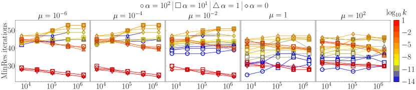
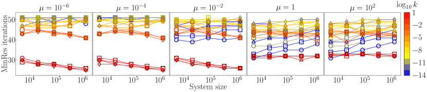
Figure 1: Performance of preconditioner (27) for the trace formulation (5) and the model problem from Example 2.1 with parameter ranges identified in Section 4.2. Discretization by $\boldsymbol{P}_{2}$-${P}_{1}$-${P}_{2}$ elements (top) and $\boldsymbol{C}\boldsymbol{R}_{1}$-${P}_{0}$-${P}_{0}$ elements (bottom) using stabilization [19] (see also (40)).

For non-conforming $\boldsymbol{C}\boldsymbol{R}_{1}$-${P}_{0}$-${P}_{0}$ elements, the results are given in the bottom panel of Fig. 1. We observe that the iterations appear bounded, varying betweeen $25$ and $51$. However, there is a modest increase with $h$ for $k=10^{-14}$ and $\mu\geq 1$. We attribute this growth to round-off errors when inverting the preconditioner since the pressure block is then scaled with $10^{-16}$-$10^{-14}$.

4.3.2 Preconditioning $\mathcal{A}^{\text{La}}$ and $\mathcal{A}^{\text{Ro}}$

We discuss robustness of (30) and (35) for the multiplier formulation (8) and the Robin formulation (10). Linear solver (MinRes) iterations over a large range of parameters are shown in Fig. 2 and confirm parameter-robustness in both cases, with iteration counts between $10$ and $39$ for (30)-preconditioned $\mathcal{A}^{\text{La}}$ and iteration counts between $1$ and $48$ for (35)-preconditioned $\mathcal{A}^{\text{Ro}}$. We note that in particular when the ratio ${\kappa}=\mu^{-1}k$ is small, the reported iteration counts are very small (even one in the most extreme case) but stable for varying system sizes. We can attribute this to the specific configuration of the test case. With ${\kappa}\ll 1$ the contribution $\beta_{n}{T^{\prime}_{n}}{T_{n}}$ in operator (31) dominates the Stokes block. We recall that $\beta_{n}:={\kappa^{-1}h_{K}}$. However, the right-hand side of the linear system only scales with $\mu$ for our particular case and both normal velocity and normal velocity gradient are zero in the exact solution (42)-(43). In this setting, the linear solver manages to reduce the very large initial defect (due the combination of random initial guess in the range $\left[0,1\right)$, large operator norm, and small right hand side) by the requested factor of $10^{8}$ in only one iteration. We remark that in this case the approximation of the solution is rather poor and a stricter convergence criterion would be required to obtain an accurate solution. However, this does not diminish the observation that the iterations are bounded. In consistency with all other results, we therefore report the results for the specified reduction of $10^{8}$. This particularity does not affect the multiplier formulation since the term $\beta_{n}{T^{\prime}_{n}}{T_{n}}$ is not present in operator (28). To fully convince the reader, we additionally report condition numbers of the discrete preconditioned operators in Appendix D. The results show that the condition number stays between $5$ and $17$ for all reported parameter combinations. We note that the condition number estimates involving $\mathcal{B}^{\text{Ro}}$ are reported over a smaller range of mesh sizes than in Fig. 2 since the computations require an expensive assembly of an inverse of sum of two inverted matrices.

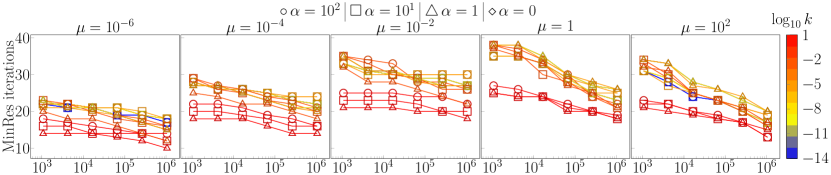
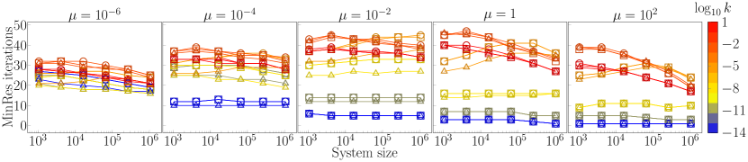
Figure 2: Iteration counts for the (30)-preconditioned multiplier formulation (8) (top) and (35)-preconditioned Robin formulation (10) (bottom). Discretization with FVM as described in Appendix A.

Preconditioners $\mathcal{B}^{\text{La}}$ and $\mathcal{B}^{\text{Ro}}$ were also investigated using non-conforming $\boldsymbol{C}\boldsymbol{R}_{1}$-${P}_{0}$-${P}_{0}$(-$P_{0}$) elements. Results collected in Fig. 3 confirm robustness of both preconditioners. The number of iterations remained between $24$ and $50$ for (30)-preconditioned $\mathcal{A}^{\text{La}}$ and between $16$ and $50$ for $\mathcal{A}^{\text{Ro}}$ with preconditioner (35).

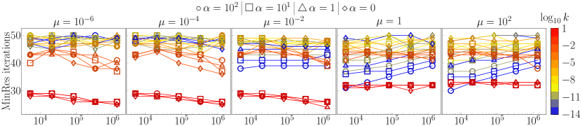
Figure 3: Iteration counts for the (30)-preconditioned Lagrange multiplier formulation (8) (top) and Robin formulation (10) with preconditioner (35) (bottom). Discretization by $\boldsymbol{C}\boldsymbol{R}_{1}$-${P}_{0}$-${P}_{0}$(-${P}_{0}$) elements.

4.4 Three-dimensional examples

The robustness study of Section 4.3 concerned a two-dimensional setup leading to a rather small interface with only a few hundred cells in $\Gamma_{h}$. Moreover, the preconditioners $\mathcal{B}^{\text{Tr}}$, $\mathcal{B}^{\text{La}}$ and $\mathcal{B}^{\text{Ro}}$ were always computed exactly. To address the efficiency of the preconditioners in more practical scenarios, we next apply the proposed Stokes-Darcy solvers to two three-dimensional model problems. In particular, we investigate the effect of approximating the action of the preconditioner blocks in terms of off-the-shelf multilevel methods. In addition, the problems are chosen such that we go beyond the assumptions on the interface (not a closed surface) and the boundary conditions (interface intersects with Neumann boundary) introduced at the end of Section 2 to simplify the theoretical analysis.

In the following two examples, we investigate solvers for two of the proposed Stokes-Darcy formulations: (A) the Trace formulation (5) with preconditioner (27) and FEM discretization and (B) the Lagrange multiplier formulation (8) with preconditioner (30) discretized by FVM. We remind the reader that the FEM and FVM implementations differ in the software stack. In particular, all FEM results using direct solvers are obtained with MUMPS [3], while FVM results use UMFPACK [26]. The FEM results rely on Hypre’s BoomerAMG [33], while for FVM the algebraic multigrid of dune-istl [13] is used. Moreover, the results are computed with different hardware setup (A) Ubuntu workstation with AMD Ryzen Threadripper 3970X 32-Core processor and 128GB of memory, (B) openSUSE workstation with AMD Ryzen Threadripper 3990X 64-Core processor and 270GB of memory. However, in both cases the computations are run in serial restricted to one CPU. Finally (and going more beyond the presented theory), the Stokes block in the FVM operators (28) and (30) is not symmetric due to a non-symmetric stencil in the current implementation of boundary condition (3a) for the case of reentrant corners in the Stokes domain. However, the asymmetry is localized to the few degrees of freedom associated with the interface. As symmetry is a strict requirement for MinRes, we present GMRes iterations instead.

To evaluate efficiency of the proposed preconditioners, we compare their numerically exact realization to approximations in terms of multilevel methods. For (A) and BoomerAMG, the different approximations correspond to computing the action of each block by increasing numbers (same for each block for simplicity) of $\text{V}(2,2)$ AMG cycles per application of the preconditioner. We used default settings except for the aggregation threshold which is set to $0.7$, the recommended value for $3d$ problems. For (B) and Dune::AMG, the number of smoother iterations $n$ on each level of a $\text{V}(n,n)$-cycle was varied.

In addition, we compare the solvers, with the analogues of the naïve precondiner presented in Example 2.1, that is, $\mathcal{B}^{\text{Tr}}$, respectively $\mathcal{B}^{\text{La}}$ with the fractional operator omitted. (Moreover, in this case the pressure block of the preconditioner reads $-{\kappa}(\Delta+I)$ to avoid the singularity due to the Neumann boundary conditions on $\partial\Omega_{D}\setminus\Gamma$.)

4.4.1 Channel flow over porous hill

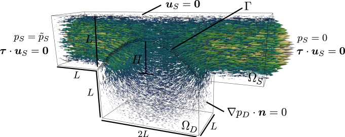
Figure 4: Setup for channel flow example in Section 4.4. All boundaries are no-flow boundaries except for the right and left sides of the channel where we prescribe pressure and zero tangential velocities with $\tilde{p}_{S}=10^{-8}\leavevmode\nobreak\$. The dimensions are given by $L=0.5$, $H=0.3$ and the interface $\Gamma$ is chosen as a section of a cylinder with radius $R=H/2+L^{2}/(2H)$. Arrows visualize the resulting velocity field for $\mu=10^{-3}$, $k=10^{-2}$, $\alpha=1$, where longer, lighter arrows correspond to higher velocities.

Table 2: Exact and approximate preconditioners for Stokes-Darcy problem in Fig. 4 using the Trace formulation (5) and preconditioner (27). Discretization by $\boldsymbol{P}_{2}$-${P}_{1}$-${P}_{2}$. MinRes iterations until convergence (reducing preconditioned residual norm by factor $10^{8}$) with the preconditioner computed exactly (bLU) and by $j\text{V}(2,2)$ cycles of AMG are shown. The numbers in parenthesis represent aggregate solver setup and solver run time rounded to full seconds. (Top) $k=10^{-2}$, (bottom) $k=10^{-5}$. In addition timings for solving $\mathcal{A}^{\text{Tr}}$ using a direct solver and preconditioned MinRes solver with the exact naïve-preconditioner of Example 2.1 are listed.

dofs	$\lvert V_{h}\rvert$	bLU	1V(2,2)	2V(2,2)	4V(2,2)	directa	naïve
3562	107	84 (1)	92 (1)	85 (1)	84 (1)	- (1)	98 (1)
13452	293	89 (2)	103 (2)	91 (3)	89 (5)	- (1)	106 (2)
69554	1023	88 (11)	112 (20)	92 (30)	88 (54)	- (4)	106 (9)
468646	3671	88 (173)	129 (265)	101 (388)	89 (646)	- (98)	108 (138)
3562	107	88 (1)	108 (1)	98 (1)	95 (1)	- (1)	1065 (2)
13452	293	92 (2)	123 (2)	106 (4)	101 (6)	- (1)	1538 (14)
69554	1023	93 (11)	143 (23)	110 (33)	98 (55)	- (4)	1659 (110)
468646	3671	97 (180)	164 (314)	122 (439)	105 (716)	- (98)	1661 (1293)

^a MUMPS

Table 3: Exact and approximate preconditioners for Stokes-Darcy problem in Fig. 4 using formulation (8) and preconditioner $\mathcal{B}^{\text{La}}$ (30). Discretization with FVM (Staggered-TPFA). GMRes iterations (reducing preconditioned residual norm by factor $10^{8}$) are shown. In parenthesis, we provide wall clock times (aggregate solver setup and runtime) rounded to full seconds. Tables shows results for $k=10^{-2}$ (top), $k=10^{-5}$ (middle), $k=10^{-12}$ (bottom). In addition timings for solving $\mathcal{A}^{\text{La}}$ using a direct solver and preconditioned GMRes solver with the exact naïve-preconditioner constructed by omission of the fractional component in $\mathcal{B}^{\text{La}}$ are included.

dofs	$|V_{h}|$	bLU	1V(1,1)	1V(2,2)	1V(4,4)	directa	naïve
8640	208	60 (1)	83 (1)	71 (1)	64 (1)	- (1)	89 (1)
66342	832	64 (11)	109 (7)	92 (7)	81 (7)	- (6)	86 (13)
517552	3264	66 (337)	156 (132)	128 (134)	109 (146)	- (468)	84 (374)
8640	208	69 (1)	111 (1)	96 (1)	89 (1)	- (1)	330 (3)
66342	832	82 (13)	145 (8)	127 (8)	112 (9)	- (6)	403 (53)
517552	3264	91 (411)	201 (161)	169 (163)	147 (180)	- (485)	449 (1431)
8640	208	69 (1)	113 (1)	97 (1)	89 (1)	- (1)	4411 (158)
66342	832	83 (14)	147 (11)	130 (11)	116 (13)	- (6)	n/cb
517552	3264	99 (437)	203 (235)	180 (256)	161 (312)	- (533)	n/cb

^a UMFPACK  ^b not converged in under $10^{\prime}000$ iterations

As the first model problem, we consider viscous flow over a porous medium with a curved interface, see Fig. 4. Let $\alpha=1$, $\mu=10^{-3}$ and $k\in\{10^{-2},10^{-5}\}$. The fluid motion is driven by a pressure difference between the inlet and outlet where the (non-standard) boundary conditions $p_{S}=\tilde{p}_{S}$ (inlet, $p_{S}=0$ on the outlet) and ${\boldsymbol{\tau}}\cdot{\boldsymbol{u}_{S}}=\boldsymbol{0}$ (see e.g. [37]) are prescribed.

On the rest of the fluid domain, we enforce ${\boldsymbol{u}_{S}}=\boldsymbol{0}$, while the boundary of the porous domain is impermeable (homogeneous Neumann boundary conditions). Therefore, newly, the interface intersects (mixed boundaries) $\Gamma^{\boldsymbol{u}}_{S}$ and $\Gamma^{u}_{D}$. The fact that $\Gamma$ is incident to the Dirichlet boundary on the Stokes side translates to a modification of the preconditioner such that the fractional operator is now constructed with Dirichlet boundary conditions, see Appendix C for further details.

Performance of the $\mathcal{B}^{\text{Tr}}$-preconditioned formulation (5) discretized with the $\boldsymbol{P}_{2}$-${P}_{1}$-${P}_{2}$ FEM is summarized in Table 2. It can be seen that exact preconditioners lead to iterations bounded in refinement with little sensitivity to the change in permeability. In addition, the LU-based preconditioners are noticeably faster than the AMG-based approximation. We remark that with LU at most 30% of the reported time was spent in the setup phase which was dominated by factorization of the blocks. To give an example of the cost of the eigensolver, for the finest interface mesh reported in Table 4, $\lvert V_{h}\rvert=13976$, assembly of the fractional block takes $256\leavevmode\nobreak\ \text{s}$. However, the presence of the resulting (large) dense block in the matrix of the pressure preconditioner also affects factorization time and the cost per Krylov iteration.

For preconditioners realized by AMG cycles robustness in $h$ requires at least four V cycles if $k=10^{-2}$ while 8 cycles are needed for $k=10^{-5}$. This result supports our observation (not reported here) that black-box algebraic multigrid is not a parameter-robust preconditioner for the pressure block in (27). Specifically, AMG struggles when the interface term dominates the Laplacian in $\Omega_{D}$. Finally, in agreement with Example 2.1 for $k=10^{-5}$, the naïve preconditioner leads to considerably more iterations (and slower run time) than $\mathcal{B}^{\text{Tr}}$. However, none of the iterative approaches outperform the direct solver for the reported system sizes.

Performance of the $\mathcal{B}^{\text{La}}$-preconditioned formulation (8) discretized with the Staggered-TPFA FVM is summarized in Table 3. In comparison with the FEM results but in consistency with observations in $2d$ examples in Section 4.3, the solvers based on FVM and exact preconditioner initially show a slight increase of the number of iterations with refinement (in particular for small $k$). However, we point out that the difference in the number of iterations between consecutive grid refinements gets smaller and smaller (similar to what can be seen for the condition numbers in Appendix D). While the solver with exact $\mathcal{B}^{\text{La}}$ appears parameter-robust, it is evident that the naïve preconditioner (missing the fractional component) is not robust in $k$. When approximating all blocks with AMG, the fastest execution times could be achieved. In comparison with BoomerAMG, Dune::AMG uses a faster but less accurate interpolation strategy, which leads to considerably faster execution time per iteration. Increasing the number of smoother iterations reduces iteration counts but due to the increased cost per iteration does not result in a better performance. Moreover, the Dune::AMG-based solver does not show robustness with grid refinement, even for a large number of smoother iterations (we tested up to $64$). However, the Dune::AMG-based solver appears robust in the model parameters.

4.4.2 Embedded porous blocks

Figure 5: Setup for porous blocks example in Section 4.4. All boundaries are no-flow boundaries except for the right and left sides of the channel where we prescribe pressure and zero tangential velocities with $\tilde{p}_{S}=10^{-8}\leavevmode\nobreak\$. The channel dimension are given by $L=0.5$ and the blocks are $\Omega_{D}^{k_{1}}=[L/2,3L/2]\times[2L/8,7L/8]\times[3L/4,7L/4]$ and $\Omega_{D}^{k_{2}}=[5L/2,7L/2]\times[L/8,6L/8]\times[1L/4,5L/4]$ and are assigned different permeabilities $k_{1}=10^{-1}$, $k_{2}=10^{-3}$. Moreover, $\mu=10^{-3}$, $\alpha=1$. The coarsest FVM discretization is a structured (anisotropic) rectangular cuboid mesh with $16\times 16\times 16$ cells. FEM results are computed with unstructured tetrahedral meshes.

Table 4: Exact and approximate preconditioners for Stokes-Darcy problem in Fig. 5 using the Trace formulation (5) and preconditioner (27). Discretization by $\boldsymbol{P}_{2}$-${P}_{1}$-${P}_{2}$. Legend as in Table 2

dofs	$\lvert V_{h}\rvert$	bLU	1V(2,2)	2V(2,2)	4V(2,2)	direct	naïve
7256	484	123 (1)	143 (2)	129 (3)	125 (4)	- (1)	240 (2)
25260	1212	125 (4)	152 (8)	131 (13)	127 (21)	- (1)	257 (6)
124732	3768	125 (37)	162 (84)	133 (127)	126 (221)	- (12)	264 (46)
836293	13976	126 (932)	189 (1426)	144 (1909)	129 (3049)	- (370)	275 (721)

Table 5: Exact and approximate preconditioners for Stokes-Darcy problem in Fig. 5 using the Lagrange multiplier formulation (8) and preconditioner (30). Discretization by FVM. Legend as in Table 3.

dofs	$\lvert V_{h}\rvert$	bLU	1V(1,1)	1V(4,4)	direct	naïve
16144	608	107 (4)	151 (3)	118 (3)	- (1)	257 (6)
122432	2432	109 (85)	192 (62)	147 (70)	- (64)	258 (138)
952576	9728	109 (3861)	281 (3458)	195 (3310)	- (5617)	187 (4806.8)

In the second and final example, we consider viscous channel flow past and through two porous inclusions with different permeabilities, see Fig. 5. From the point of view of assumptions of Section 2, the novel feature is the fact that the interface is now formed by two closed surfaces.

Iterations counts and runtime estimates for various solvers are shown in Table 4 (FEM) and Table 5 (FVM). In general, the conclusions from Section 4.4.1 apply to the new example as well. In particular, exact preconditioners $\mathcal{B}^{\text{Tr}}$, $\mathcal{B}^{\text{Tr}}$ yield iteration counts that are stable in mesh size.

5 Conclusions and outlook

Our work concerned monolithic preconditioning of symmetric formulations of the coupled Stokes-primal Darcy problem which were motivated by differences in handling the interface coupling that are natural to finite element and finite volume methods. Parameter robust preconditioners for each of the three formulations were constructed based on the well-posedness of the problems established within a unifying functional framework. The proposed preconditioners are based on norms in fractional Sobolev spaces. Using discretization in terms of both FEM and FVM our numerical results demonstrated the parameter-robustness in several examples partly going beyond the presented theory in terms of boundary conditions and interface configuration. However, efficiency of the proposed solvers is currently sub-optimal due to the realization of the pressure preconditioner, in particular, the reliance on the spectral form of the fractional interface operators.

To improve efficiency of the proposed preconditioners scalable techniques for the parameter-robust approximation of the components, in particular, the pressure block, will be addressed in the future work. To possibly improve the efficiency further, the use of lower/upper-triangular preconditioners or approximations of full Schur complement factorizations could be investigated. Here, a reduction of the iteration count is expected but the cost-benefit ratio of such an approach for the presented cases remains to be seen. Finally, extensions of the proposed preconditioners to more complex physics such as the Navier-Stokes-Darcy problem may be addressed in future work.

Appendix A Non-conforming discretizations

This section provides additional details on discretization of the Stokes-Darcy operators by lowest-order non-conforming FEM (i.e. $\boldsymbol{C}\boldsymbol{R}_{1}$ elements for the space ${\boldsymbol{V}}_{S,h}$ and ${P}_{0}$ elements for $Q_{D,h}$) and FVM. In the following we denote as $\mathcal{F}^{i}(\Omega_{h})$ the set of interior facets of a given mesh $\Omega_{h}$ of generic bounded Lipschitz domain $\Omega$.

Non-conforming finite element discretization

To obtain stable discretization of the Stokes subproblem in (5)-(10) on the space ${\boldsymbol{V}}_{S,h}={\boldsymbol{V}}_{S,h}(\Omega_{h})$ constructed in terms of Crouzeix-Raviart $\boldsymbol{C}\boldsymbol{R}_{1}$ element we employ the facet stabilization [19]. That is, the operator $-\nabla\cdot(2\mu{\boldsymbol{\epsilon}})$ is discretized as

(40) $$\langle-\nabla\cdot(2\mu{\boldsymbol{\epsilon}}({\boldsymbol{u}})),{\boldsymbol{v}}\rangle:=(2\mu\boldsymbol{\epsilon}({\boldsymbol{u}}),\boldsymbol{\epsilon}({\boldsymbol{v}}))_{\Omega}+\sum_{F\in\mathcal{F}^{i}({\Omega_{h}})}(\frac{2\mu}{\lvert F\rvert}[\![{\boldsymbol{u}}]\!],[\![{\boldsymbol{v}}]\!])_{F},\quad\forall{\boldsymbol{u}},{\boldsymbol{v}}\in{\boldsymbol{V}}_{h},$$

where $[\![\boldsymbol{u}]\!]=\boldsymbol{u}|_{K^{+}}-\boldsymbol{u}|_{K^{-}}$ in which $K^{\pm}$ denote the two cells sharing the facet $F$. Moreover, we recall that $\mu$ is assumed to be constant and that $h_{K}$ measures the distance between facet midpoint and centroids/circumcenters of the connected cells.

Approximation of the Laplace operator in the space of piece-wise constant functions $Q_{h}=Q_{h}(\Omega_{h})$ uses a two-point flux approximation, that is, we let

$$\langle-\Delta p,q\rangle:=\sum_{F\in\mathcal{F}^{i}({\Omega_{h}})}(\frac{1}{2\left\{\!\!\left\{h_{K}\right\}\!\!\right\}}[\![p]\!],[\![q]\!])_{F}+(h_{K}^{-1}p,q)_{\Gamma^{p}},\quad\forall p,q\in Q_{D},$$

where $[\![{p}]\!]={p}|_{K^{+}}-{p}|_{K^{-}}$, $\left\{\!\!\left\{p\right\}\!\!\right\}=\tfrac{1}{2}(p|_{K^{+}}+p|_{K^{-}})$, and $\Gamma^{p}\subseteq\partial\Omega$ is the part of the domain boundary with Dirichlet data. This definition is also used when assembling the fractional operator via the eigenvalue problems in (36) and in Appendix C.

Finite volume discretization

The herein employed finite volume discretization method (FVM) is a combination of a staggered face-centered finite volume scheme (Staggered) for the Stokes momentum balance equation (2a) and a cell-centered finite volume scheme with two-point flux approximation (TPFA) for the Stokes mass balance equation (2b), the Darcy equation (1) and, if using the Lagrange multiplier formulation, eigenvalue problem (36). For the description of the Staggered FVM, we refer to [40, 64, 63]. Here, due to the immediate relevance for the construction of the Lagrange multiplier and Robin formulations (8) and (10) as well as the assembly of eigenvalue problem (36), we briefly review the cell-centered TPFA FVM.

Let us consider as example the Darcy equation (1). We integrate (1) over each control volume ${K}\in\Omega_{D,h}$, apply the divergence theorem and approximate the interface fluxes by a discrete numerical flux approximation $\Psi_{K,F}$ for each face $F$ of $K$,

$$-\int_{\partial{K}}\mu^{-1}k\nabla p_{D}\cdot\boldsymbol{n}_{{K},F}\,\textrm{d}s=\int_{{K}}f_{D}\,\textrm{d}x\quad\Rightarrow\quad\sum\limits_{F\in\partial K}\Psi_{K_{D},F}=\lvert{K}\rvert f_{D}(\boldsymbol{x}_{K}),$$

where $\boldsymbol{n}_{{K},F}$ is a unit normal vector on $F$ pointing out of $K$ and $\boldsymbol{x}_{K}$ is the centroid of ${K}$. A two-point flux approximation for $\Psi_{K_{D},F}$ on inner facets is then given by

(41) $$\Psi_{{K},{F}}:=\frac{1}{\mu}\frac{t_{{K},{F}}t_{L,{F}}}{t_{{K},{F}}+t_{L,{F}}}(p_{K}-p_{L}),\quad t_{{K},{F}}:=k_{K}\frac{\boldsymbol{d}_{{{K}},{F}}\cdot\boldsymbol{n}_{{K},{F}}}{||\boldsymbol{d}_{{K},{F}}||^{2}}\lvert{F}\rvert,$$

where $p_{K}$ denotes the average cell pressure in cell ${K}$, $k_{K}$ the permeability of cell $K$, $\boldsymbol{d}_{{K},{F}}$ the vector connecting $\boldsymbol{x}_{K}$ and an integration point on $F$ (e.g. centroid), and $L$ is a neighboring cell sharing $F$ with $K$. Note that (41) also applies for surface grids, for instance, for the approximation of eigenvalue problem (36) on curved surfaces. On the boundary, we either specify $\Psi_{{K},{F}}$ directly (Neumann boundary conditions) or compute $\Psi_{{K},{F}}=\mu^{-1}k_{K}t_{{K},{F}}(p_{K}-p_{\partial{K}})$ where $p_{\partial{K}}$ is the given boundary data on $F\subset\partial\Omega_{D}$. (That is, Dirichlet data, or interface pressure $p_{\Gamma}$ in the case of the coupling interface.) We remark that approximation (41) is only consistent on $\boldsymbol{K}$-orthogonal grids [1].

Appendix B Numerical tests and manufactured solution

For the numerical grid convergence tests and parameter-robustness tests, we work with the manufactured solution given in [64] for unit parameters $\mu=1$, $k=1$, $\alpha=1$ as

(42a) $${\boldsymbol{u}_{S}} =\begin{bmatrix}-\frac{1}{\pi}\exp(x_{2})\sin(\pi x_{1})\\ (\exp(x_{2})-\exp(1))\cos(\pi x_{1})\end{bmatrix} \text{in}\quad\Omega_{S},$$

(42b) $$p_{S} =2\exp(x_{2})\cos(\pi x_{1}), \text{in}\quad\Omega_{S},$$

(42c) $$p_{D} =(\exp(x_{2})-x_{2}\exp(1))\cos(\pi x_{1}) \text{in}\quad\Omega_{D},$$

where $$\Omega_{D}=[0,1]\times[0,1] \Omega_{F}=[0,1]\times[1,2]$$, . Moreover, for the formulation with Lagrange multiplier,

(42d) $$\lambda =p_{D}(x_{1},x_{2}=1)=0 \text{on}\quad\Gamma,$$

where $\Gamma=[0,1]\times\{1\}$. To obtain the same solution over the whole range of parameters, we use the following source terms

(43a) $${\boldsymbol{f}_{S}} :=\begin{bmatrix}\frac{1}{\pi}\exp(x_{2})\sin(\pi x_{1})(\mu-\mu\pi^{2}-2\pi^{2})\\ \cos(\pi x_{1})(\mu\left((\pi^{2}+1)\exp(x_{2})-\pi^{2}\exp(1))\right)+2(1-\mu)\exp(x_{2}))\end{bmatrix},$$

(43b) $$f_{D} :=\frac{k}{\mu}\cos(\pi x_{1})\left((\pi^{2}+1)\exp(x_{2})-\pi^{2}x_{2}\exp(1)\right),$$

and modified coupling conditions

(44a) $${\boldsymbol{\tau}}\cdot{\boldsymbol{\sigma}({\boldsymbol{u}_{S}},p_{S})}\cdot{\boldsymbol{n}}+{\beta_{\tau}}{\boldsymbol{\tau}}\cdot{\boldsymbol{u}_{S}} =h^{\Gamma}_{\tau}, h^{\Gamma}_{\tau}:=\left({\beta_{\tau}}-\mu\right)\frac{1}{\pi}\exp(x_{2})\sin(\pi x_{1}),$$

(44b) $${\boldsymbol{n}}\cdot{\boldsymbol{\sigma}({\boldsymbol{u}_{S}},p_{S})}\cdot{\boldsymbol{n}}+{p}_{D} =h^{\Gamma}_{n}, h^{\Gamma}_{n}:=2(\mu-1)\exp(1)\cos(\pi x_{1}),$$

(44c) $${\boldsymbol{u}_{S}}\cdot{\boldsymbol{n}}+{\kappa}\nabla p_{D}\cdot{\boldsymbol{n}} =g^{\Gamma}, g^{\Gamma}:=0.$$

The functions $h^{\Gamma}_{\tau}$, $h^{\Gamma}_{n}$, and $g^{\Gamma}$ ensure that the conditions are satisfied independent of the choice of parameters. Note that the choice of data in (44) only modifies the right-hand side while the problem operators remain unchanged.

This setting enables code verification in terms of grid convergence tests in all parameter settings. For grid convergence tests, the errors for the finite element schemes are reported in $L^{2}$ and $H^{1}$ norms. Using $\boldsymbol{P}_{2}$-$P_{1}$-$P_{2}$ elements for (5) quadratic convergence in all the variables in their respective norms is expected. Discretization by $\boldsymbol{C}\boldsymbol{R}_{1}$-$P_{0}$-$P_{0}$(-$P_{0}$) in all the formulations yields a first order scheme.

The errors for the finite volume scheme are computed in the following discrete $L^{2}$ norm

(45) $$\lVert u\rVert_{\text{FV}}:=\left(\sum\limits_{K\in{\Omega}_{h}}|K|u_{K}^{2}\right)^{\frac{1}{2}}.$$

It is well known that with the typical flux reconstruction schemes, based on a two-point flux approximation on structured Cartesian grids, second order super-convergence at cell centers (pressures) and face centers (Stokes velocity components) is obtained [51, 31, 62].

We report error convergence of the FEM schemes for all the formulations in Fig. 6. Expected (or faster) convergence is observed in all cases. We remark that the observed quadratic convergence of the interfacial pressure $p|_{\Gamma}$ in (8) is likely due to the zero exact solution in the manufactured setup. Error convergence for the FVM schemes is reported for formulations (8) and (10) in Fig. 7. Quadratic convergence in the discrete norm (45) is observed for all the variables.

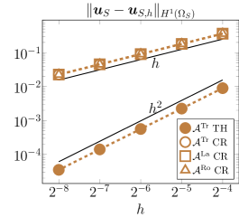
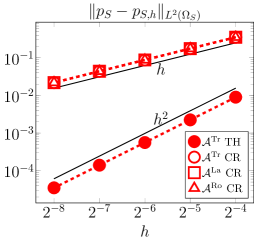
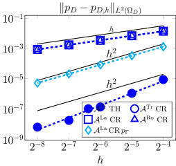
Figure 6: Approximation properties of FEM discretizations for the manufactured problem (42) with unit parameters using the Trace formulation (5), multiplier formulation (8) and Robin formulation (10). Only (5) is considered with $\boldsymbol{P}_{2}$-$P_{1}$-$P_{2}$ while $\boldsymbol{C}\boldsymbol{R}_{1}$-$P_{0}$-$P_{0}$(-$P_{0}$) is used for all formulations. $L^{2}(\Gamma)$-error of interface pressure in (8) is plotted in cyan color.

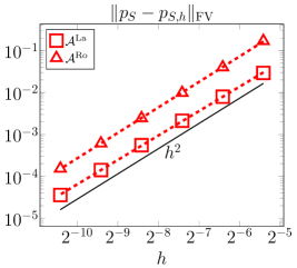
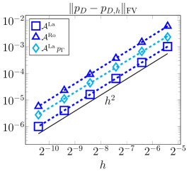
Figure 7: Approximation properties of FVM (Staggered-TPFA) discretization for the manufactured problem (42) with unit parameters using the Lagrange multiplier formulation (8) and the Robin formulation (10). $u_{S,x}$ and $u_{S,y}$ denote the components of ${\boldsymbol{u}_{S}}$ (the degrees of freedom for the respective components have different locations and control volumes in the staggered FVM). For (8) the error of interface pressure error measured in $L^{2}$-norm (45) on $\Gamma$ is plotted in cyan.

Appendix C Interface intersecting Dirichlet boundaries

The analysis of Section 3 and robustness study of Section 4.3 assume that the interface $\Gamma$ intersects the Neumann boundaries of both the Darcy and the Stokes domain. This fact was reflected by the $\|\cdot\|_{-\frac{1}{2},\Gamma}$ norm used in the analysis and in the preconditioner construction through eigenvalue problem (36). If instead, $\Gamma$ intersects the Dirichlet boundaries of the respective problems (27) no longer defines a parameter-robust preconditioner for formulation (5), see Table 6.

Table 6: Condition numbers of (27)-preconditioned $\mathcal{A}^{\text{Tr}}$ when $\Gamma$ intersects Dirichlet boundaries of both subproblems. Geometry of Example 2.1 is used with $\mu=1$, $\alpha=1$. Parameter sensitivity is due to incorrect, namely, $\lVert\cdot\rVert_{-\frac{1}{2},\Gamma}$, control at the interface.

	$2^{-2}$	$2^{-3}$	$2^{-4}$	$2^{-5}$	$2^{-6}$
$1$	7.37	7.46	7.47	7.46	7.45
$10^{-1}$	9.16	9.26	9.27	9.26	9.26
$10^{-2}$	18.21	18.52	18.58	18.59	18.58
$10^{-4}$	30.59	34.94	37.84	39.13	39.51

However, the theory of Section 3 and resulting preconditioners can be extended to more general cases. In particular, the fact that $\Gamma$ intersects with Dirichlet boundaries translates into a modification of the interface norm to be used in the preconditioner, that is, the pressure on the interface shall be controlled in $\|\cdot\|_{H^{-\frac{1}{2}}_{00}(\Gamma)}$. We recall that $H^{\frac{1}{2}}_{00}(\Gamma)$ is a subspace of $H^{\frac{1}{2}}(\partial\Omega_{D})$ containing functions that vanish on $\partial\Omega_{D}\setminus\Gamma$, see [35] for more details. Hence, eigenvalue problem (36) used in the construction of the discrete preconditioner is replaced by $-\Delta_{\Gamma}u=\lambda u$ on $\Gamma$ and $u=0$ on $\partial\Gamma$, i.e. Dirichlet conditions are enforced. Finally, we note that above we have set $\mu=1$ for simplicity. In general case, the parameter scaling is analogous to (36).

Using $\boldsymbol{P}_{2}$-$P_{1}$-$P_{2}$ elements, Fig. 8 reports spectral condition numbers of the Stokes-Darcy Trace formulation (5) with preconditioner (27). The geometry is taken from Example 2.1, however for the Dirichlet case, the placement of Dirichlet and Neumann boundaries is interchanged: Neumann boundaries on top and bottom edges; Dirichlet boundary conditions on the lateral edges which intersect with $\Gamma$. Parameter ranges from Section 4.2 are used. We observe stable condition numbers $C$ in the range $7.3\leq C\leq 18.5$ (interface meeting Dirichlet boundary) and $6.2\leq C\leq 16.5$ (interface meeting Neumann boundaries, i.e. the case analyzed in Section 3 and numerically investigated in Section 4).

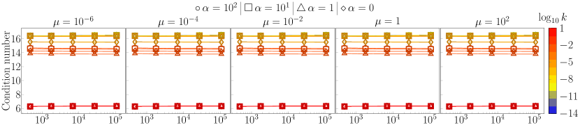
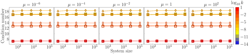
Figure 8: Condition numbers for (27)-preconditioned formulation (5) across the parameter ranges from Section 4.2, with interface $\Gamma$ intersecting Neumann boundaries (top) or Dirichlet boundaries (bottom). The case of Dirichlet boundaries requires modification of the preconditioner as described in Appendix C. Problem (5) is assembled on geometry defined in Example 2.1 and discretized by $\boldsymbol{P}_{2}$-$P_{1}$-$P_{2}$ elements.

Appendix D FVM condition numbers for $\mathcal{B}^{\text{La}}$ and $\mathcal{B}^{\text{Ro}}$

We report in Fig. 9 the condition numbers corresponding to the numerical tests of Section 4.3 and the MinRes iteration results reported in Section 4.3.2.

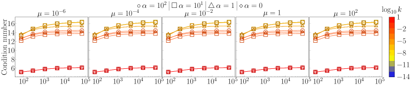
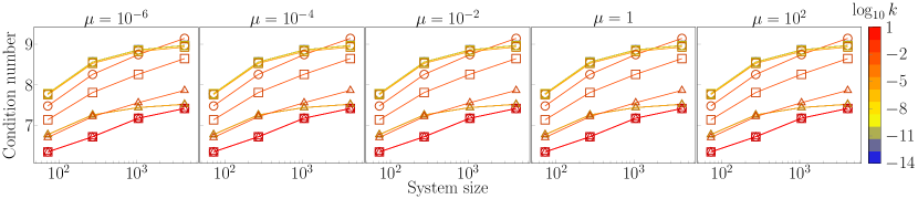
Figure 9: Condition numbers for the (30)-preconditioned multiplier formulation (8) and the (35)-preconditioned FVM formulation (10) (bottom) across the parameter ranges from Section 4.2. Both formulations are discretized with FVM (Appendix A). Not all $k$ are visible since the data overlaps with larger values of $k$.

References

- [1] I. Aavatsmark, T. Barkve, O. Bøe, and T. Mannseth, Discretization on unstructured grids for inhomogeneous, anisotropic media. Part I: Derivation of the methods, SIAM Journal on Scientific Computing, 19 (1998), pp. 1700–1716, https://doi.org/10.1137/s1064827595293582.
- [2] S. Ackermann, C. Bringedal, and R. Helmig, Multi-scale three-domain approach for coupling free flow and flow in porous media including droplet-related interface processes, Journal of Computational Physics, 429 (2021), p. 109993, https://doi.org/10.1016/j.jcp.2020.109993.
- [3] P. Amestoy, I. S. Duff, J. Koster, and J.-Y. L’Excellent, A fully asynchronous multifrontal solver using distributed dynamic scheduling, SIAM Journal on Matrix Analysis and Applications, 23 (2001), pp. 15–41.
- [4] K. Baber, K. Mosthaf, B. Flemisch, R. Helmig, S. Muthing, and B. Wohlmuth, Numerical scheme for coupling two-phase compositional porous-media flow and one-phase compositional free flow, IMA Journal of Applied Mathematics, 77 (2012), pp. 887–909, https://doi.org/10.1093/imamat/hxs048.
- [5] S. Badia and R. Codina, Unified stabilized finite element formulations for the Stokes and the Darcy problems, SIAM journal on Numerical Analysis, 47 (2009), pp. 1971–2000.
- [6] T. Bærland, M. Kuchta, and K.-A. Mardal, Multigrid methods for discrete fractional Sobolev spaces, SIAM Journal on Scientific Computing, 41 (2019), pp. A948–A972.
- [7] T. Bærland, M. Kuchta, K.-A. Mardal, and T. Thompson, An observation on the uniform preconditioners for the mixed darcy problem, Numerical Methods for Partial Differential Equations, 36 (2020), pp. 1718–1734.
- [8] S. Balay, S. Abhyankar, M. F. Adams, et al., PETSc/TAO users manual, Tech. Report ANL-21/39 - Revision 3.16, Argonne National Laboratory, 2021.
- [9] P. Bastian, M. Blatt, A. Dedner, C. Engwer, R. Klöfkorn, R. Kornhuber, M. Ohlberger, and O. Sander, A generic grid interface for parallel and adaptive scientific computing. part II: Implementation and tests in DUNE, Computing, 82 (2008), pp. 121–138, https://doi.org/10.1007/s00607-008-0004-9.
- [10] G. S. Beavers and D. D. Joseph, Boundary conditions at a naturally permeable wall, Journal of Fluid Mechanics, 30 (1967), pp. 197–207, https://doi.org/10.1017/s0022112067001375.
- [11] J. Bergh and J. Löfström, Interpolation Spaces: An Introduction, Grundlehren der mathematischen Wissenschaften, Springer Berlin Heidelberg, 2012.
- [12] N. Birgle, R. Masson, and L. Trenty, A domain decomposition method to couple nonisothermal compositional gas liquid darcy and free gas flows, Journal of Computational Physics, 368 (2018), pp. 210–235, https://doi.org/10.1016/j.jcp.2018.04.035.
- [13] M. Blatt, A Parallel Algebraic Multigrid Method for Elliptic Problems with Highly Discontinuous Coefficients, PhD thesis, University of Heidelberg, Germany, 2010, https://doi.org/10.11588/HEIDOK.00010856.
- [14] M. Blatt and P. Bastian, The iterative solver template library, in Applied Parallel Computing. State of the Art in Scientific Computing: 8th International Workshop, PARA 2006, Umeå, Sweden, June 18-21, 2006, Revised Selected Papers, Berlin, Heidelberg, 2007, Springer Berlin Heidelberg, pp. 666–675, https://doi.org/10.1007/978-3-540-75755-9_82.
- [15] W. Boon, M. Kuchta, K.-A. Mardal, and R. Ruiz-Baier, Robust preconditioners and stability analysis for perturbed saddle-point problems – application to conservative discretizations of Biot’s equations utilizing total pressure, SIAM Journal on Scientific Computing, 43 (2021), pp. B961–B983.
- [16] Boon, W. M., A parameter-robust iterative method for Stokes-Darcy problems retaining local mass conservation, ESAIM: M2AN, 54 (2020), pp. 2045–2067.
- [17] D. Braess, Stability of saddle point problems with penalty, ESAIM: Mathematical Modelling and Numerical Analysis - Modélisation Mathématique et Analyse Numérique, 30 (1996), pp. 731–742.
- [18] J. Bramble, J. Pasciak, and P. Vassilevski, Computational scales of Sobolev norms with application to preconditioning, Mathematics of Computation, 69 (2000), pp. 463–480.
- [19] E. Burman and P. Hansbo, Stabilized Crouzeix-Raviart element for the Darcy-Stokes problem, Numerical Methods for Partial Differential Equations, 21 (2005), pp. 986–997, https://doi.org/https://doi.org/10.1002/num.20076.
- [20] E. Burman and P. Hansbo, A unified stabilized method for Stokes’ and Darcy’s equations, Journal of Computational and Applied Mathematics, 198 (2007), pp. 35–51.
- [21] M. Cai, M. Mu, and J. Xu, Preconditioning techniques for a mixed Stokes/Darcy model in porous media applications, Journal of computational and applied mathematics, 233 (2009), pp. 346–355.
- [22] A. Caiazzo, V. John, and U. Wilbrandt, On classical iterative subdomain methods for the Stokes–Darcy problem, Computational Geosciences, 18 (2014), pp. 711–728.
- [23] W. Chen, M. Gunzburger, F. Hua, and X. Wang, A parallel Robin–Robin domain decomposition method for the Stokes–Darcy system, SIAM Journal on Numerical Analysis, 49 (2011), pp. 1064–1084.
- [24] P. Chidyagwai, S. Ladenheim, and D. B. Szyld, Constraint preconditioning for the coupled Stokes–Darcy system, SIAM Journal on Scientific Computing, 38 (2016), pp. A668–A690.
- [25] E. Coltman, M. Lipp, A. Vescovini, and R. Helmig, Obstacles, interfacial forms, and turbulence: A numerical analysis of soil–water evaporation across different interfaces, Transport in Porous Media, 134 (2020), pp. 275–301, https://doi.org/10.1007/s11242-020-01445-6.
- [26] T. A. Davis, Algorithm 832: UMFPACK V4.3 - an unsymmetric-pattern multifrontal method, ACM Transactions on Mathematical Software (TOMS), 30 (2004), pp. 196–199, https://doi.org/10.1145/992200.992206.
- [27] M. Discacciati and L. Gerardo-Giorda, Optimized Schwarz methods for the Stokes–Darcy coupling, IMA Journal of Numerical Analysis, 38 (2018), pp. 1959–1983.
- [28] M. Discacciati, E. Miglio, and A. Quarteroni, Mathematical and numerical models for coupling surface and groundwater flows, Applied Numerical Mathematics, 43 (2002), pp. 57–74.
- [29] M. Discacciati and A. Quarteroni, Navier-Stokes/Darcy coupling: modeling, analysis, and numerical approximation, Rev. Mat. Complut, 22 (2009), pp. 315–426.
- [30] M. Discacciati, A. Quarteroni, and A. Valli, Robin–Robin domain decomposition methods for the Stokes–Darcy coupling, SIAM Journal on Numerical Analysis, 45 (2007), pp. 1246–1268.
- [31] J. Droniou and N. Nataraj, Improved estimate for gradient schemes and super-convergence of the TPFA finite volume scheme, IMA Journal of Numerical Analysis, 38 (2017), pp. 1254–1293, https://doi.org/10.1093/imanum/drx028.
- [32] A. Ern and J.-L. Guermond, Theory and practice of finite elements, vol. 159, Springer Science & Business Media, 2013.
- [33] R. D. Falgout and U. M. Yang, hypre: A library of high performance preconditioners, in Computational Science — ICCS 2002, P. M. A. Sloot, A. G. Hoekstra, C. J. K. Tan, and J. J. Dongarra, eds., Berlin, Heidelberg, 2002, Springer Berlin Heidelberg, pp. 632–641.
- [34] T. Führer, Multilevel decompositions and norms for negative order Sobolev spaces, Mathematics of Computation, (2021).
- [35] J. Galvis and M. Sarkis, Non-matching mortar discretization analysis for the coupling Stokes-Darcy equations, Electron. Trans. Numer. Anal, 26 (2007), p. 07.
- [36] G. N. Gatica, S. Meddahi, and R. Oyarzúa, A conforming mixed finite-element method for the coupling of fluid flow with porous media flow, IMA Journal of Numerical Analysis, 29 (2008), pp. 86–108.
- [37] V. Girault, Curl-conforming finite element methods for Navier-Stokes equations with non-standard boundary conditions in , in The Navier-Stokes Equations Theory and Numerical Methods, Springer, 1990, pp. 201–218.
- [38] V. Girault, D. Vassilev, and I. Yotov, Mortar multiscale finite element methods for Stokes–Darcy flows, Numerische Mathematik, 127 (2014), pp. 93–165.
- [39] G. Guennebaud, B. Jacob, et al., Eigen v3. http://eigen.tuxfamily.org, 2010.
- [40] F. H. Harlow and J. E. Welch, Numerical calculation of time-dependent viscous incompressible flow of fluid with free surface, Physics of Fluids, 8 (1965), p. 2182, https://doi.org/10.1063/1.1761178.
- [41] V. Hernandez, J. E. Roman, and V. Vidal, SLEPc: A scalable and flexible toolkit for the solution of eigenvalue problems, ACM Trans. Math. Software, 31 (2005), pp. 351–362.
- [42] K. E. Holter, B. Kehlet, A. Devor, T. J. Sejnowski, et al., Interstitial solute transport in 3d reconstructed neuropil occurs by diffusion rather than bulk flow, Proceedings of the National Academy of Sciences, 114 (2017), pp. 9894–9899, https://doi.org/10.1073/pnas.1706942114.
- [43] K. E. Holter, M. Kuchta, and K.-A. Mardal, Robust preconditioning of monolithically coupled multiphysics problems, arXiv preprint arXiv:2001.05527, (2020).
- [44] Q. Hong, J. Kraus, M. Lymbery, and F. Philo, A new framework for the stability analysis of perturbed saddle-point problems and applications in poromechanics, arXiv preprint arXiv:2103.09357, (2021).
- [45] T. Karper, K.-A. Mardal, and R. Winther, Unified finite element discretizations of coupled Darcy–Stokes flow, Numerical Methods for Partial Differential Equations: An International Journal, 25 (2009), pp. 311–326.
- [46] T. Koch, B. Flemisch, R. Helmig, R. Wiest, and D. Obrist, A multiscale subvoxel perfusion model to estimate diffusive capillary wall conductivity in multiple sclerosis lesions from perfusion mri data, International Journal for Numerical Methods in Biomedical Engineering, 36 (2020), p. e3298, https://doi.org/https://doi.org/10.1002/cnm.3298.
- [47] T. Koch, D. Gläser, K. Weishaupt, et al., DuMux 3 - an open-source simulator for solving flow and transport problems in porous media with a focus on model coupling, Computers & Mathematics with Applications, (2020), https://doi.org/10.1016/j.camwa.2020.02.012.
- [48] M. Kuchta, Assembly of multiscale linear PDE operators, in Numerical Mathematics and Advanced Applications ENUMATH 2019, F. J. Vermolen and C. Vuik, eds., Cham, 2021, Springer International Publishing, pp. 641–650.
- [49] M. Kuchta, M. Nordaas, J. Verschaeve, M. Mortensen, and K. Mardal, Preconditioners for saddle point systems with trace constraints coupling 2d and 1d domains, SIAM Journal on Scientific Computing, 38 (2016), pp. B962–B987.
- [50] W. J. Layton, F. Schieweck, and I. Yotov, Coupling fluid flow with porous media flow, SIAM Journal on Numerical Analysis, 40 (2002), pp. 2195–2218.
- [51] J. Li and S. Sun, The superconvergence phenomenon and proof of the MAC scheme for the Stokes equations on non-uniform rectangular meshes, Journal of Scientific Computing, 65 (2014), pp. 341–362, https://doi.org/10.1007/s10915-014-9963-5.
- [52] P. Luo, C. Rodrigo, F. J. Gaspar, and C. W. Oosterlee, Uzawa smoother in multigrid for the coupled porous medium and Stokes flow system, SIAM J. Sci. Comput., 39 (2017).
- [53] K.-A. Mardal and R. Winther, Preconditioning discretizations of systems of partial differential equations, Numerical Linear Algebra with Applications, 18 (2011), pp. 1–40, https://doi.org/10.1002/nla.716.
- [54] A. Mikelić and W. Jäger, On The Interface Boundary Condition of Beavers, Joseph, and Saffman, SIAM Journal on Applied Mathematics, 60 (2000), pp. 1111–1127, https://doi.org/10.1137/s003613999833678x.
- [55] K. Mosthaf, K. Baber, B. Flemisch, R. Helmig, A. Leijnse, I. Rybak, and B. Wohlmuth, A coupling concept for two-phase compositional porous-medium and single-phase compositional free flow, Water Resources Research, 47 (2011), https://doi.org/doi.org/10.1029/2011WR010685.
- [56] P. Oswald, Multilevel norms for , Computing, 61 (2007), pp. 235–255.
- [57] Y. Qiu, Spectra. https://github.com/yixuan/spectra, 2019.
- [58] B. Rivière, Analysis of a discontinuous finite element method for the coupled Stokes and Darcy problems, J. Sci. Comput., 22–23 (2005), p. 479–500, https://doi.org/10.1007/s10915-004-4147-3.
- [59] B. Rivière and I. Yotov, Locally conservative coupling of Stokes and Darcy flows, SIAM Journal on Numerical Analysis, 42 (2005), pp. 1959–1977.
- [60] E. Rohan, J. Turjanicová, and V. Lukeš, Multiscale modelling and simulations of tissue perfusion using the Biot-Darcy-Brinkman model, Computers & Structures, 251 (2021), p. 106404, https://doi.org/https://doi.org/10.1016/j.compstruc.2020.106404.
- [61] P. G. Saffman, On the boundary condition at the surface of a porous medium, Studies in Applied Mathematics, 50 (1971), pp. 93–101, https://doi.org/10.1002/sapm197150293.
- [62] M. Schneider, D. Gläser, B. Flemisch, and R. Helmig, Comparison of finite-volume schemes for diffusion problems, Oil & Gas Science and Technology – Revue d’IFP Energies nouvelles, 73 (2018), p. 82, https://doi.org/10.2516/ogst/2018064.
- [63] M. Schneider, K. Weishaupt, D. Gläser, W. M. Boon, and R. Helmig, Coupling staggered-grid and MPFA finite volume methods for free flow/porous-medium flow problems, Journal of Computational Physics, 401 (2020), p. 109012, https://doi.org/10.1016/j.jcp.2019.109012.
- [64] M.-C. Shiue, K. C. Ong, and M.-C. Lai, Convergence of the MAC scheme for the Stokes/Darcy coupling problem, Journal of Scientific Computing, 76 (2018), pp. 1216–1251, https://doi.org/10.1007/s10915-018-0660-7.
- [65] J. H. Smith and J. A. Humphrey, Interstitial transport and transvascular fluid exchange during infusion into brain and tumor tissue, Microvascular research, 73 (2007), pp. 58–73.
- [66] R. Stevenson and R. van Venetië, Uniform preconditioners of linear complexity for problems of negative order, Computational Methods in Applied Mathematics, 21 (2021), pp. 469–478, https://doi.org/doi:10.1515/cmam-2020-0052, https://doi.org/10.1515/cmam-2020-0052.
- [67] A. Terzis, I. Zarikos, K. Weishaupt, G. Yang, X. Chu, R. Helmig, and B. Weigand, Microscopic velocity field measurements inside a regular porous medium adjacent to a low reynolds number channel flow, Physics of Fluids, 31 (2019), p. 042001, https://doi.org/10.1063/1.5092169.