Inferring manifolds from noisy data using Gaussian processes

Abstract.

In analyzing complex datasets, it is often of interest to infer lower dimensional structure underlying the higher dimensional observations. As a flexible class of nonlinear structures, it is common to focus on Riemannian manifolds. Most existing manifold learning algorithms replace the original data with lower dimensional coordinates without providing an estimate of the manifold in the observation space or using the manifold to denoise the original data. This article proposes a new methodology for addressing these problems, allowing interpolation of the estimated manifold between fitted data points. The proposed approach is motivated by novel theoretical properties of local covariance matrices constructed from noisy samples on a manifold. Our results enable us to turn a global manifold reconstruction problem into a local regression problem, allowing application of Gaussian processes for probabilistic manifold reconstruction. In addition to theory justifying the algorithm, we provide simulated and real data examples to illustrate the performance.

1. Introduction

Data are often observed as moderate to high-dimensional but in many cases have a lower dimensional structure. As this structure may be non-linear, it is common to characterize it mathematically as a Riemannian manifold. This has led to a rich literature on manifold learning algorithms, which reconstruct the observed data in a low dimensional space, while maintaining as much of the topology and geometry of the underlying manifold as possible. Some well known manifold learning algorithms include isomap [30], Laplacian eigenmaps [3], locally linear embeddings [26], diffusion maps [7] and t-distributed stochastic neighbor embedding [31]. In practice, for the manifold assumption to be realistic, it is typically necessary to allow measurement error. Although some manifold learning algorithms are robust to noise [12, 27, 11, 8], these algorithms focus on providing lower-dimensional features and not on estimating the manifold or providing fitted values in the original sample space. The goal of this article is to address these limitations of classical manifold learning algorithms.

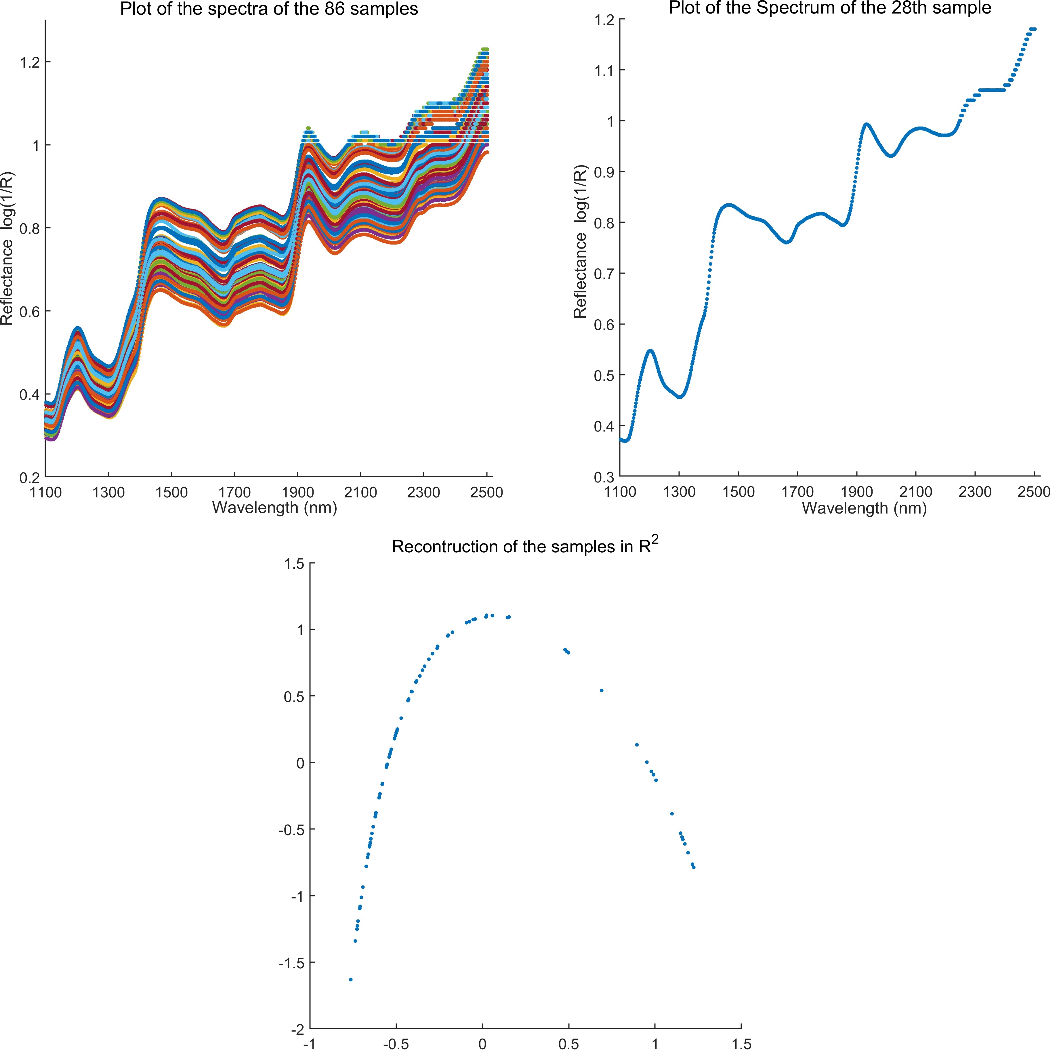
We use the following example as illustration. Near-infrared reflectance spectroscopy (NIRS) is widely used to assess food quality. The relation between wavelengths of incident waves and diffuse reflectance of the waves is called the reflectance spectrum, which relates to water content, sugar content and ripeness of crops. We consider the reflectance spectra for $86$ wheat samples, with the near-infrared waves measured in $2$ nm intervals from $1100$ nm to $2500$ nm. Each of the $86$ samples can be represented as a point in $\mathbb{R}^{701}$ with each coordinate the reflectance of the corresponding incident wave. We plot the data in Figure 1, which shows that the observed reflectances are noisy, especially over the wavelengths from $1900$ nm to $2500$nm. We first apply diffusion maps [7], producing a reconstruction in $\mathbb{R}^{2}$ revealing an underlying one dimensional manifold structure. While diffusion maps may be useful for learning very low-dimensional features summarizing NIRS data, it is unclear how these features relate to the original spectrum data, limiting interpretability. It would be appealing to have an approach that can infer the manifold structure in the original $\mathbb{R}^{701}$ spectra space, while exploiting the manifold structure to denoise the data.

Figure 1. Top Left Panel: The near-infrared reflectance spectra of 86 wheat samples. The observed reflectance is noisy, especially over wavelengths from $1900$ nm to $2500$nm. Top Right Panel: The plot of the spectrum of the $28$th sample. Bottom Panel: Representing each spectrum at a point in $\mathbb{R}^{701}$ and applying diffusion maps, we obtain a curve in $\mathbb{R}^{2}$.

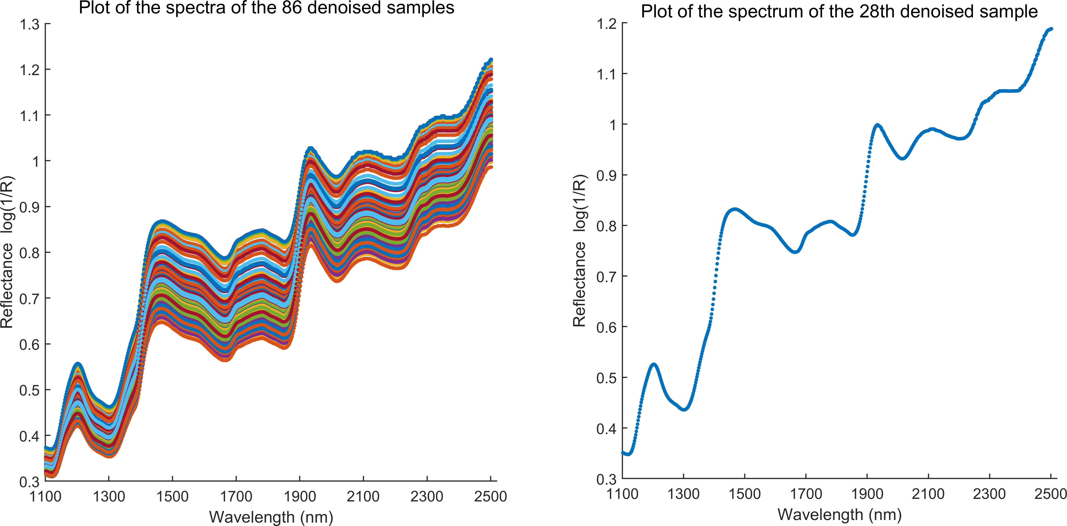
In this article, we propose a Manifold reconstruction via Gaussian processes (MrGap) algorithm, which estimates a submanifold of the observation space from samples on the manifold corrupted by Gaussian noise. MrGap builds upon our theoretical analysis of the spectral behavior of the local covariance matrix of noisy samples on a manifold. Our theoretical results enable us to turn a global manifold reconstruction problem into a local regression problem so that we can apply Gaussian process (GP) regression. The predictors and the response variables of the regression problem are constructed from the Euclidean coordinates of the noisy samples. MrGap provides a probabilistic method to reconstruct a manifold in the sense that for each noisy sample, we obtain a probability distribution whose mean is a denoised point on the manifold. Moreover, we can interpolate between different denoised points. To provide a teaser illustrating practical advantages of our algorithm, we apply the algorithm to the reflectance spectra example. The $86$ spectra in $\mathbb{R}^{701}$ are denoised in a way that incorporates the underlying manifold structure. We plot the reflectance spectra in Figure 2.

Figure 2. Left: Denoised near-infrared reflectance spectra of $86$ wheat samples obtained by applying the proposed MrGap algorithm. Right: The plot of the denoised spectrum of the $28$th sample.

We briefly review some related literature. The spectral properties of the local covariance matrix constructed from samples on an embedded submanifold in Euclidean space have been extensively studied. [28] analyzes the bias and variance of the local covariance matrix constructed by a smooth kernel supported on $[0,1]$, assuming samples without noise from a closed submanifold. [33, 34] study spectral behavior of the local covariance matrix constructed from a $0-1$ kernel, assuming samples without noise from a closed submanifold and a submanifold with a boundary. [19] studies the local covariance matrix constructed from $k$ nearest neighbors, assuming the embedded submanifold can be locally parametrized by quadratic functions in the tangent spaces and samples are images of uniform samples in the domain of their parameterization with Gaussian noise. This is a quite restricted setting, and we consider much more general sampling conditions. Our theory on the local covariance matrix generalizes [33] to allow Gaussian noise.

In addition to manifold learning algorithms that reconstruct a data set in a low dimensional space, there are also algorithms developed to reconstruct a manifold from noisy samples in the original high dimensional space. [24] propose an algorithm to recover the homology groups of the manifold, assuming samples fall in an $\epsilon$ neighborhood of the manifold. [16] assumes noise in the normal direction to the manifold, developing a method similar to [24] and proving the convergence rate when the variance of the noise is known. The principal curve algorithm is an iterative method to fit a curve through the data [17, 20, 21]. [29] and [22] propose principal manifold methods extending principal curves to higher dimensions. [14, 15] consider samples from a manifold with Gaussian noise. By using the partition of unity, they construct a vector bundle in the neighborhood of the samples to approximate the normal bundle of the manifold. The manifold is reconstructed in a determinisitic way by using the vector bundle. [1] and [2] apply local polynomial fitting to reconstruct a manifold from noisy samples. [1] assumes bounded noise in the normal direction, while [2] consider uniformly distributed noise in a tubular neighborhood of the manifold.

The rest of the paper is organized as follows. We set up the problem formally and describe the goals in section 2. In section 2.1, we define the local covariance matrix and the associated projection operators. In section 2.2, we briefly review GP regression. In section 2.3, we propose the MrGap algorithm with an explanation in section 2.4. Theoretical analysis of MrGap is in section 3. In section 3.1, we introduce geometric preliminaries. We provide a bias and variance analysis of the local covariance matrix in section 3.2. In section 3.3, we construct the charts of a manifold based on the projection operators associated with the local covariance matrix. In section 3.4, we relate the reconstruction of the chart to a regression problem. In section 3.5, we discuss the algorithm theoretically based on the previous results. In section 3.6, we introduce a geometric root mean square error to evaluate algorithm performance. The numerical simulations are in section 4. In section 5, we apply the algorithm to the reflectance spectra of wheat data.

We summarize our notation. Let $\{e_{i}\}_{i=1}^{D}$ be the standard orthonormal basis of $\mathbb{R}^{D}$, where $e_{i}=[0,\cdots,1,\cdots,0]^{\top}$ with $1$ in the $i$-th entry. Similarly, let $\{e^{\prime}_{i}\}_{i=1}^{d}$ be the standard orthonormal basis of $\mathbb{R}^{d}$. Let $J\in\mathbb{R}^{D\times d}$ be a projection matrix such that $J_{ij}=1$ when $i=j$ and $J_{ij}=0$ when $i\not=j$. Let $\bar{J}\in\mathbb{R}^{D\times(D-d)}$ be another projection matrix such that $\bar{J}_{ij}=1$ when $i=d+j$ and $\bar{J}_{ij}=0$ otherwise. If $\iota$ is an isometric embedding of a manifold $M$ into $\mathbb{R}^{D}$, then $\iota_{*}$ is the push forward map of $\iota$. For $x\in M$, $T_{x}M$ is the tangent space of $M$ at $x$ and $\iota_{*}T_{x}M$ is the tangent space of $\iota(M)$ at $\iota(x)$. We use $B^{\mathbb{R}^{d}}_{r}$ and $B^{\mathbb{R}^{D}}_{r}$ to denote open balls of radius $r$ in $\mathbb{R}^{d}$ and $\mathbb{R}^{D}$, respectively. We use bold lowercase letters to denote Euclidean vectors.

2. Manifold Reconstruction via Gaussian Processes

In this section, we propose an algorithm to reconstruct an embedded submanifold of Euclidean space from noisy samples. We first make the following assumption about the samples.

Assumption 1.

Let $M$ be a $d$-dimensional smooth, closed and connected Riemannian manifold isometrically embedded in $\mathbb{R}^{D}$ through $\iota:M\to\mathbb{R}^{D}$. The observed data, $\textbf{y}_{i}\in\mathbb{R}^{D}$ for $i=1,\ldots,n,$ can be expressed as $\textbf{y}_{i}=\iota(x_{i})+\eta_{i}$, where $x_{i}$ are i.i.d sampled from $\mathsf{P}$ and $\eta_{i}$ are i.i.d sampled from $\mathcal{N}(0,\sigma^{2}I_{D\times D})$ independently of $x_{i}$. Here, $(M,\mathcal{F},\mathsf{P})$ is a probability space, where $\mathsf{P}$ is a probability measure defined over the Borel sigma algebra $\mathcal{F}$ on $M$. We assume $\mathsf{P}$ is absolutely continuous with respect to the volume measure on $M$, i.e. $d\mathsf{P}=PdV$ by the Radon-Nikodym theorem, where $P$ is the probability density function on $M$ and $dV$ is the volume form. We further assume $P$ is smooth and is bounded from below by $P_{m}>0$ and bounded from above by $P_{M}$.

In this work, the embedded submanifold $\iota(M)$ is not accessible and we are only given the Euclidean coordinates of $\{\textbf{y}_{i}\}_{i=1}^{n}$. We want to develop an algorithm to achieve the following two goals:

1. For each $\textbf{y}_{k}$, find a corresponding $\hat{\textbf{y}}_{k}\in\iota(M)$ while controlling $\frac{1}{n}\sum_{i=1}^{n}\|\iota(x_{i})-\hat{\textbf{y}}_{i}\|^{2}_{\mathbb{R}^{D}}$.

2. For each $\hat{\textbf{y}}_{k}$, find a chart of $\iota(M)$ around $\hat{\textbf{y}}_{k}$ so that we can interpolate on $\iota(M)$.

For simplicity, we consider the dimension $d$ of the manifold as known throughout the paper. Under Assumption 1, we provide a method to determine the dimension $d$ in Appendix F. There are two major ingredients in our algorithm: the local covariance matrix and GP regression. Before we describe the algorithm, we review these ingredients briefly in the following two subsections.

2.1. Local covariance matrix

Letting $\chi(t)=1$ for $t\in[0,1]$ and $\chi(t)=0$ for $t>1$ denote a $0-1$ kernel, we define a local covariance matrix at a sample point $\textbf{y}_{k}$ based on data $\{\textbf{y}_{1},\cdots,\textbf{y}_{n}\}\subset\mathbb{R}^{D}$,

(1) $$C_{n,\epsilon}(\textbf{y}_{k})=\frac{1}{n}\sum_{i=1}^{n}(\textbf{y}_{i}-\textbf{y}_{k})(\textbf{y}_{i}-\textbf{y}_{k})^{\top}\chi\Big{(}\frac{\|\textbf{y}_{i}-\textbf{y}_{k}\|_{\mathbb{R}^{D}}}{\epsilon}\Big{)},$$

where $\epsilon>0$, and $C_{n,\epsilon}$ is the covariance matrix used in local Principal Components Analysis (PCA); $C_{n,\epsilon}$ and its eigenvectors are major ingredients of our algorithm. Consider the eigen decomposition

(2) $$C_{n,\epsilon}(\textbf{y}_{k})=U_{n,\epsilon}(\textbf{y}_{k})\Lambda_{n,\epsilon}(\textbf{y}_{k})U_{n,\epsilon}(\textbf{y}_{k})^{\top},$$

with $U_{n,\epsilon}(\textbf{y}_{k})\in\mathbb{O}(D)$ and $\Lambda_{n,\epsilon}(\textbf{y}_{k})\in\mathbb{R}^{D\times D}$ a diagonal matrix containing the eigenvalues of $C_{n,\epsilon}(\textbf{y}_{k})$ in decreasing order on the diagonal, $e_{1}^{\top}\Lambda_{n,\epsilon}(\textbf{y}_{k})e_{1}\geq e_{2}^{\top}\Lambda_{n,\epsilon}(\textbf{y}_{k})e_{2}\geq\cdots\geq e_{D}^{\top}\Lambda_{n,\epsilon}(\textbf{y}_{k})e_{D}$. The column vectors of $U_{n,\epsilon}(\textbf{y}_{k})$ are the orthonormal eigenvectors of $C_{n,\epsilon}(\textbf{y}_{k})$ corresponding to decreasing order of the eigenvalues. The eigenvectors form an orthonormal basis of $\mathbb{R}^{D}$. We define projection operators from $\mathbb{R}^{D}$ onto two subspaces as follows. For any $\textbf{y}\in\mathbb{R}^{D}$, let

(3) $$\mathcal{P}_{\textbf{y}_{k}}(\textbf{y})=J^{\top}U_{n,\epsilon}(\textbf{y}_{k})^{\top}(\textbf{y}-\textbf{y}_{k}),$$

be the projection onto the subspace generated by the first $d$ column vectors of $U_{n,\epsilon}(\textbf{y}_{k})$. Let

(4) $$\mathcal{P}^{\bot}_{\textbf{y}_{k}}(\textbf{y}):=\bar{J}^{\top}U_{n,\epsilon}(\textbf{y}_{k})^{\top}(\textbf{y}-\textbf{y}_{k}),$$

be the projection onto the subspace generated by the last $D-d$ column vectors of $U_{n,\epsilon}(\textbf{y}_{k})$.

2.2. Gaussian process regression

Suppose $F:\mathbb{R}^{d}\rightarrow\mathbb{R}^{q}$ is an unknown regression function with $F=(f_{1},\cdots,f_{q})$. Letting $\textbf{z}_{i}\in\mathbb{R}^{q}$ denote the response vector and $\textbf{u}_{i}\in\mathbb{R}^{d}$ denote the predictor vector, for $i=1,\ldots,n$, and allowing for measurement error, we let

(5) $$\textbf{z}_{i}=F(\textbf{u}_{i})+\eta_{i},\qquad\eta_{i}\sim\mathcal{N}(0,\sigma^{2}I_{q\times q}).$$

We assign a GP prior to each component function $f_{j}$ with mean $0$ and covariance function

(6) $$\mathsf{C}(\textbf{u},\textbf{u}^{\prime})=A\exp\Big{(}-\frac{\|\textbf{u}-\textbf{u}^{\prime}\|^{2}_{\mathbb{R}^{d}}}{\rho}\Big{)}.$$

Denote $\textbf{f}_{j}\in\mathbb{R}^{N}$ to be the discretization of $f_{j}$ over $\{\textbf{u}_{i}\}_{i=1}^{N}$ so that $\textbf{f}_{j}(i)=f_{j}(\textbf{u}_{i})$ for $j=1,\ldots,q$. A GP prior for $f_{j}$ implies $p(\textbf{f}_{j}|\textbf{u}_{1},\textbf{u}_{2},\cdots,\textbf{u}_{N})=\mathcal{N}(0,\Sigma_{1})$, where $\Sigma_{1}\in\mathbb{R}^{N\times N}$ is the covariance matrix induced from $\mathsf{C}$, with the $(j,k)$ element of $\Sigma_{1}$ corresponding to $\mathsf{C}(\textbf{u}_{j},\textbf{u}_{k})$, for $1\leq j,k\leq N$. Prior distribution $\mathcal{N}(0,\Sigma_{1})$ can be combined with information in the likelihood function under model (5) to obtain the posterior distribution, which will be used as a basis for inference.

Suppose we want to predict $F$ at $\{\textbf{u}_{i}\}_{i=N+1}^{N+m}$. Denote $\textbf{f}^{*}_{j}\in\mathbb{R}^{m}$ with $\textbf{f}^{*}_{j}(i)=f_{j}(\textbf{u}_{N+i})$ for $j=1,\ldots,q$ and $i=1,\ldots,m$. Under a GP prior for $f_{j}$, the joint distribution of $\textbf{f}_{j}$ and $\textbf{f}^{*}_{j}$ is $p(\textbf{f}_{j},\textbf{f}^{*}_{j})=\mathcal{N}(0,\Sigma),$ where $\Sigma=\begin{bmatrix}\Sigma_{1}&\Sigma_{2}\\ \Sigma_{3}&\Sigma_{4}\end{bmatrix}\,,$ with $\Sigma_{2}\in\mathbb{R}^{N\times m}$, $\Sigma_{3}\in\mathbb{R}^{m\times N}$, and $\Sigma_{4}\in\mathbb{R}^{m\times m}$ induced from covariance function $\mathsf{C}$. Denote $\textbf{F}\in\mathbb{R}^{m\times q}$ with $j$th column $\textbf{f}^{*}_{j}$ and denote $\textbf{Z}\in\mathbb{R}^{N\times q}$ with $i$th row $\textbf{z}_{i}$. Under model (5) and a GP prior, we have $p(\textbf{Z},\textbf{F})=\mathcal{N}(0,\tilde{\Sigma}),$ where

$$\tilde{\Sigma}=\Sigma+\begin{bmatrix}\sigma^{2}I_{N\times N}&0\\ 0&0\\ \end{bmatrix}=\begin{bmatrix}\Sigma_{1}+\sigma^{2}I_{N\times N}&\Sigma_{2}\\ \Sigma_{3}&\Sigma_{4}\\ \end{bmatrix}.$$

By direct calculation, the predictive distribution is

(7) $$p(\textbf{F}|\textbf{Z})=\mathcal{N}(\Sigma_{3}(\Sigma_{1}+\sigma^{2}I_{N\times N})^{-1}\textbf{Z},\Sigma_{4}-\Sigma_{3}(\Sigma_{1}+\sigma^{2}I_{N\times N})^{-1}\Sigma_{2})\,.$$

The covariance parameters $A$, $\rho$ and $\sigma$ can be estimated by maximizing the natural log of the marginal likelihood, obtained by marginalizing over the GP prior,

(8) $$\log p(\textbf{Z}|A,\rho,\sigma)=-\mathrm{tr}(\textbf{Z}^{\top}(\Sigma_{1}+\sigma^{2}I_{N\times N})^{-1}\textbf{Z})-q\log(\det(\Sigma_{1}+\sigma^{2}I_{N\times N}))-\frac{qN}{2}\log(2\pi).$$

This empirical Bayes approach for parameter estimation automatically protects against over-fitting. Refer to [25] for more background on GP regression.

2.3. MrGap algorithm

From Assumption 1, $\textbf{y}_{i}=\iota(x_{i})+\eta_{i}$ with $\textbf{y}_{i}$ a noisy version of data $\iota(x_{i})$, for $i=1,\cdots,n$. Algorithm 1 uses GP regression to iteratively denoise each data point $\textbf{y}_{i}$ relying on data in a local neighborhood around that point. The output of Algorithm 1 is the denoised data $\{\hat{\textbf{y}}_{1},\cdots,\hat{\textbf{y}}_{n}\}$. Inputs include data $\{\textbf{y}_{i}\}_{i=1}^{n}$, a bandwidth $\epsilon$ of the local covariance matrix in (1), and a scale $\delta$ of the projection maps (3) and (4). The bandwidth $\epsilon$ is chosen so that each $B^{\mathbb{R}^{D}}_{\epsilon}(\textbf{y}_{k})\cap\{\textbf{y}_{1},\cdots,\textbf{y}_{n}\}$ has more than $d$ points and $\delta>\epsilon$.

1 For each $\textbf{y}_{k}$, construct $C_{n,\epsilon}(\textbf{y}_{k})$ as in (1). Denote the $N_{k}$ samples in $B^{\mathbb{R}^{D}}_{\delta}(\textbf{y}_{k})$ as $\{\textbf{y}_{k,1},\cdots,\textbf{y}_{k,N_{k}}\}$. Let $\textbf{w}_{k,j}=\mathcal{P}_{\textbf{y}_{k}}(\textbf{y}_{k,j})$ and $\textbf{z}_{k,j}=\mathcal{P}^{\bot}_{\textbf{y}_{k}}(\textbf{y}_{k,j})$ for $j=1,\cdots,N_{k}$, with $\mathcal{P}_{\textbf{y}_{k}}(\textbf{y})$ and $\mathcal{P}^{\bot}_{\textbf{y}_{k}}(\textbf{y})$ defined in (3) and (4). The $k$th local GP regression has responses $\textbf{z}_{k,j}$ and predictors $\textbf{w}_{k,j}$.

2For each $\textbf{y}_{k}$, construct covariance $\Sigma_{k}=\begin{bmatrix}\Sigma_{k,1}&\Sigma_{k,2}\\ \Sigma_{k,3}&\Sigma_{k,4}\end{bmatrix}\in\mathbb{R}^{(N_{k}+1)\times(N_{k}+1)}$ over $\{\textbf{w}_{k,1},\cdots,\textbf{w}_{k,N_{k}},0\}$ induced by $\mathsf{C}$ in (6), with $\Sigma_{k,1}\in\mathbb{R}^{N_{k}\times N_{k}}$. Denote $\textbf{Z}_{k}\in\mathbb{R}^{N_{k}\times(D-d)}$ with $i$th row $\textbf{z}_{k,i}$.

3For the $k$th local GP regression, the log marginal likelihood is calculated using (8) for $\textbf{Z}=\textbf{Z}_{k}$, $\Sigma_{1}=\Sigma_{k,1}$ and $N=N_{k}$. We choose $A$, $\rho$ and $\sigma$ to maximize the sum of these log marginal likelihoods over $k=1,\ldots,n$,

(9) $$\sum_{k=1}^{n}\log p_{k}(\textbf{Z}_{k}|A,\rho,\sigma)=- \sum_{k=1}^{n}\Big{(}\mathrm{tr}(\textbf{Z}_{k}^{\top}(\Sigma_{k,1}+\sigma^{2}I_{N_{k}\times N_{k}})^{-1}\textbf{Z}_{k})$$

$$-(D-d)\log(\det(\Sigma_{k,1}+\sigma^{2}I_{N_{k}\times N_{k}}))-\frac{qN_{k}}{2}\log(2\pi)\Big{)}.$$

We then obtain the denoised output data using

(10) $$\textbf{y}^{(1)}_{k}=\textbf{y}_{k}+U_{n,\epsilon}(\textbf{y}_{k})\begin{bmatrix}0\\ (\Sigma_{k,3}(\Sigma_{k,1}+{\sigma}^{2}I_{N_{k}\times N_{k}})^{-1}\textbf{Z}_{k})^{\top}\\ \end{bmatrix},$$

where $U_{n,\epsilon}(\textbf{y}_{k})$ is the orthonormal eigenvector matrix of $C_{n,\epsilon}(\textbf{y}_{k})$ defined in (2).

Repeat Steps 1-3 using the denoised data in Step 3 as the input in Step 1. Stop iterating when the change in $\sigma$ between iterations is below a small tolerance and output the final denoised data.

Algorithm 1 MrGap denoising steps to produce estimates of $\hat{\textbf{y}}_{1},\cdots,\hat{\textbf{y}}_{n}$ from $\textbf{y}_{1},\ldots,\textbf{y}_{n}$.

After data denoising to infer points $\{\hat{\textbf{y}}_{1},\cdots,\hat{\textbf{y}}_{n}\}$, the second phase of our MrGap algorithm is to interpolate $K$ points around each $\hat{\textbf{y}}_{k}$ on $\iota(M)$. This interpolation phase is described in Algorithm 2. Inputs consist of $K$, the values of $A,\rho,\sigma$ from Algorithm 1, and the denoised data $\{\textbf{y}_{1},\cdots,\textbf{y}_{n}\}$ from the second to last round of Algorithm 1. Algorithm 2 iteratively interpolates $K$ points around each $\hat{\textbf{y}}_{k}$ for $k=1,\ldots,n$.

1 for $k=1,\cdots,n$ do

2       Let $\tilde{M}_{k-1}$ be the union of the $K(k-1)$ points already interpolated around $\{\hat{\textbf{y}}_{1},\cdots,\hat{\textbf{y}}_{k-1}\}$. For notation simplicity, we use $\{\textbf{y}_{1},\cdots,\textbf{y}_{n}\}$ to denote the denoised output from the second to last round iteration in Algorithm 1.

3      Use $\{\textbf{y}_{1},\cdots,\textbf{y}_{n}\}$ to repeat Step 1 of Algorithm 1. Construct $C_{n,\epsilon}(\textbf{y}_{k})$ and find $U_{n,\epsilon}(\textbf{y}_{k})$. Obtain $\textbf{z}_{k,j},\textbf{w}_{k,j}$, for $j=1,\cdots,N_{k}$.

4      Let $\mathcal{U}_{k}=\frac{1}{N_{k}}\sum_{j=1}^{N_{k}}\textbf{w}_{k,1},$ and $(m_{k},s_{k})$ denote the mean and standard deviation of $\{\|\textbf{w}_{k,1}-\mathcal{U}_{k}\|_{\mathbb{R}^{d}},\cdots,\|\textbf{w}_{k,N_{k}}-\mathcal{U}_{k}\|_{\mathbb{R}^{d}}\}$. Let $\{\tilde{\textbf{u}}_{k,1},\cdots,\tilde{\textbf{u}}_{k,K}\}$ be $K$ samples generated uniformly in $B^{\mathbb{R}^{d}}_{m_{k}-s_{k}}(\mathcal{U}_{k})$. Suppose $B^{\mathbb{R}^{D}}_{\delta}(\textbf{y}_{k})\cap\tilde{M}_{k-1}=\{\tilde{\textbf{y}}_{k,1},\cdots,\tilde{\textbf{y}}_{k,L_{k}}\}$, and let $\tilde{\textbf{w}}_{k,j}=\mathcal{P}_{\textbf{y}_{k}}(\tilde{\textbf{y}}_{k,j})$, $\tilde{\textbf{z}}_{k,j}=\mathcal{P}^{\bot}_{\textbf{y}_{k}}(\tilde{\textbf{y}}_{k,j})$ for $j=1,\cdots,L_{k}$.

5      Construct covariance $\tilde{\Sigma}_{k}=\begin{bmatrix}\tilde{\Sigma}_{k,1}&\tilde{\Sigma}_{k,2}\\ \tilde{\Sigma}_{k,3}&\tilde{\Sigma}_{k,4}\end{bmatrix}$ over $\{\textbf{w}_{k,1},\cdots,\textbf{w}_{k,N_{k}},\tilde{\textbf{w}}_{k,1},\cdots,\tilde{\textbf{w}}_{k,L_{k}},\tilde{\textbf{u}}_{k,1},\cdots,\tilde{\textbf{u}}_{k,K}\}$ using covariance $\mathsf{C}$ in (6) and the covariance parameters that we find in the last round iteration of Algorithm 1, with $\tilde{\Sigma}_{k,1}$ corresponding to $\{\textbf{w}_{k,1},\cdots,\textbf{w}_{k,N_{k}},\tilde{\textbf{w}}_{k,1},\cdots,\tilde{\textbf{w}}_{k,L_{k}}\}$. Denote $\textbf{Z}_{k}\in\mathbb{R}^{N_{k}\times(D-d)}$ with $j$th row $\textbf{z}_{k,j}$, and $\tilde{\textbf{Z}}_{k}\in\mathbb{R}^{L_{k}\times(D-d)}$ with $j$th row $\tilde{\textbf{z}}_{k,j}$.

6      Let $\textbf{1}_{K}$ denote a $K$-vector of ones. Then, the column vectors of

(11) $$\textbf{y}_{k}\textbf{1}^{\top}_{K}+U_{n,\epsilon}(\textbf{y}_{k})\begin{bmatrix}\tilde{\textbf{u}}_{k,1},\cdots,\tilde{\textbf{u}}_{k,K}\\ \Big{(}\tilde{\Sigma}_{k,3}(\tilde{\Sigma}_{k,1}+{\sigma}^{2}I_{(N_{k}+L_{k})\times(N_{k}+L_{k})})^{-1}\begin{bmatrix}\textbf{Z}_{k}\\ \tilde{\textbf{Z}}_{k}\end{bmatrix}\Big{)}^{\top}\\ \end{bmatrix}\in\mathbb{R}^{D\times K},$$

give the Euclidean coordinates of the points that we interpolate around $\hat{\textbf{y}}_{k}$.

7 end for

Algorithm 2 MrGap steps to iteratively interpolate $K$ points around each $\hat{\textbf{y}}_{k}$.

2.4. Motivation for algorithm

We provide an intuitive justification for the MrGap algorithm; a more formal theoretical discussion is in Section 3. We start from Algorithm 1. Let $\mathcal{H}_{k}$ and $\mathcal{A}_{k}$ be the affine subspaces through $\textbf{y}_{k}$ generated by the first $d$ and last $D-d$ eigenvectors of $C_{n,\epsilon}(\textbf{y}_{k})$, respectively. It can be shown that under certain relations between the bandwidth $\epsilon$ of the local covariance matrix, the variance of the noise $\sigma^{2}$, and the sample size $n$, with high probability, for $\delta>\epsilon$ and any $\textbf{y}_{k}$, $B^{\mathbb{R}^{D}}_{2\delta}(\textbf{y}_{k})\cap\iota(M)$ can be parametrized as the graph of a function: $F_{k}(\textbf{u}):O_{k}\rightarrow\mathbb{R}^{D-d}$ up to a rotation and a translation in $\mathbb{R}^{D}$, where $O_{k}$ is an open set in $\mathbb{R}^{d}$. The left panel in Figure 3 provides an illustration. Specifically, $B^{\mathbb{R}^{D}}_{2\delta}(\textbf{y}_{k})\cap\iota(M)$ can be parametrized as

$$\textbf{y}_{k}+U_{n,\epsilon}(\textbf{y}_{k})\begin{bmatrix}\textbf{u}\\ F_{k}(\textbf{u})\\ \end{bmatrix}$$

for $\textbf{u}\in O_{k}$ and $U_{n,\epsilon}(\textbf{y}_{k})$ defined in (2). If we can recover the function $F_{k}$, then we can recover $\iota(M)$ locally. In particular, since $\mathcal{P}_{\textbf{y}_{k}}(\textbf{y}_{k})=0$,

$$\textbf{y}_{k}+U_{n,\epsilon}(\textbf{y}_{k})\begin{bmatrix}0\\ F_{k}(0)\\ \end{bmatrix}$$

is the prediction of a point on $\iota(M)$ corresponding to $\textbf{y}_{k}$, which is the initial denoised output. Observe that $\textbf{w}_{k,j}=\mathcal{P}_{\textbf{y}_{k}}(\textbf{y}_{k,j})$ for $j=1,\cdots,N_{k}$ are the inputs for $F_{k}$ and $\textbf{z}_{k,j}=\mathcal{P}^{\bot}_{\textbf{y}_{k}}(\textbf{y}_{k,j})$ for $j=1,\cdots,N_{k}$ are the corresponding response variables. These inputs can be identified as the points

(12) $$\textbf{y}_{k}+U_{n,\epsilon}(\textbf{y}_{k})\begin{bmatrix}\textbf{w}_{k,j}\\ 0\\ \end{bmatrix}$$

for $j=1,\cdots,N_{k}$ in $\mathcal{H}_{k}$. In Step 1 of Algorithm 1, we construct the inputs and response variables, in Step 2 we calculate the GP covariance matrix, and in Step 3 we apply GP regression, while estimating the tuning parameters, to recover $F_{k}(0)$ in order to denoise the data. Recovery of $F_{k}$ involves a challenging errors in variables regression problem, so that it becomes necessary to apply Step 4 of Algorithm 1 to iteratively refine the results from Steps 1 to 3; Step 4 is further motivated in Section 3.

Figure 3. Red and purple lines represent affine subspaces $\mathcal{H}_{k}$ and $\mathcal{A}_{k}$, respectively. The manifold can be parameterized locally as the graph of a function whose domain is in $\mathcal{H}_{k}$. Left panel: black points are data in $B^{\mathbb{R}^{D}}_{\delta}(\textbf{y}_{k})$. The cyan points are the projections of these data onto $\mathcal{H}_{k}$ expressed as in (12). Right panel: In this case $\sigma\approx 0$ and MrGap stops after the first round. We focus our discussion on the point $\textbf{y}_{2}$. The pink points $\hat{\textbf{y}}_{1}$ and $\hat{\textbf{y}}_{2}$ are the denoised outputs for $\textbf{y}_{1}$ and $\textbf{y}_{2}$ respectively. We interpolated $K$ points around $\hat{\textbf{y}}_{1}$ on $\iota(M)$; $\tilde{M}_{1}$ is the union of these $K$ points. To interpolate $K$ points around $\hat{\textbf{y}}_{2}$ on $\iota(M)$, we find $\tilde{M}_{1}\cap B^{\mathbb{R}^{D}}_{\delta}(\textbf{y}_{2})$ which are the orange points. Interpolation is then based on a GP which uses the green points as inputs and the projections of the black points in $B^{\mathbb{R}^{D}}_{\delta}(\textbf{y}_{2})$ and the orange points onto $\mathcal{A}_{2}$ as response variables.

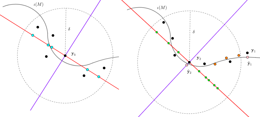
Next, we discuss Algorithm 2. For simplicity, suppose $\sigma\approx 0$, so that the variance of the noise is very small and one iteration in Algorithm 1 suffices. We interpolate $K$ points iteratively around each denoised output $\hat{\textbf{y}}_{k}$ on $\iota(M)$ for $k$ from $1$ to $n$. We use the inputs $\textbf{w}_{k,j}$ for $j=1,\cdots,N_{k}$ to estimate a small round ball contained in the domain $O_{k}$ with the center of the ball the mean of $\{\textbf{w}_{k,j}\}_{j=1}^{N_{k}}$. We uniformly randomly sample $K$ points $\{\tilde{\textbf{u}}_{k,1},\cdots,\tilde{\textbf{u}}_{k,K}\}$ in the ball; $\{\tilde{\textbf{u}}_{k,1},\cdots,\tilde{\textbf{u}}_{k,K}\}$ can be identified as the points

(13) $$\textbf{y}_{k}+U_{n,\epsilon}(\textbf{y}_{k})\begin{bmatrix}\tilde{\textbf{u}}_{k,j}\\ 0\\ \end{bmatrix}$$

for $j=1,\cdots,K$ in $\mathcal{H}_{k}$. The $K$ points are interpolated in $B^{\mathbb{R}^{D}}_{2\delta}(\textbf{y}_{k})\cap\iota(M)$ through the parametrization of $B^{\mathbb{R}^{D}}_{2\delta}(\textbf{y}_{k})\cap\iota(M)$. Hence,

$$\textbf{y}_{k}+U_{n,\epsilon}(\textbf{y}_{k})\begin{bmatrix}\tilde{\textbf{u}}_{k,j}\\ F_{k}(\tilde{\textbf{u}}_{k,j})\\ \end{bmatrix}$$

is a point interpolated in $B^{\mathbb{R}^{D}}_{2\delta}(\textbf{y}_{k})\cap\iota(M)$ for $j=1,\cdots,K$. However, it is possible that $B^{\mathbb{R}^{D}}_{2\delta}(\textbf{y}_{k})\cap\iota(M)$ and $B^{\mathbb{R}^{D}}_{2\delta}(\textbf{y}_{k^{\prime}})\cap\iota(M)$ intersect when $k\not=k^{\prime}$. We want to make sure that the points interpolated in $B^{\mathbb{R}^{D}}_{2\delta}(\textbf{y}_{k})\cap\iota(M)$ and $B^{\mathbb{R}^{D}}_{2\delta}(\textbf{y}_{k^{\prime}})\cap\iota(M)$ are glued together smoothly along the intersecting region. Suppose we interpolated $K(k-1)$ points around $\hat{\textbf{y}}_{1},\cdots,\hat{\textbf{y}}_{k-1}$ and we denote the union of these points as $\tilde{M}_{k-1}$. We explain how to interpolate $K$ points in $B^{\mathbb{R}^{D}}_{2\delta}(\textbf{y}_{k})\cap\iota(M)$ and glue them smoothly with $\tilde{M}_{k-1}$. We find $\tilde{M}_{k-1}\cap B^{\mathbb{R}^{D}}_{\delta}(\textbf{y}_{k})=\{\tilde{\textbf{y}}_{k,1},\cdots,\tilde{\textbf{y}}_{k,L_{k}}\}$. We use both $\textbf{w}_{k,j}=\mathcal{P}_{\textbf{y}_{k}}(\textbf{y}_{k,j})$ for $j=1,\cdots,N_{k}$ and $\tilde{\textbf{w}}_{k,j}=\mathcal{P}_{\textbf{y}_{k}}(\tilde{\textbf{y}}_{k,j})$ for $j=1,\cdots L_{k}$ as the inputs for $F_{k}$. We use both $\textbf{z}_{k,j}=\mathcal{P}^{\bot}_{\textbf{y}_{k}}(\textbf{y}_{k,j})$ for $j=1,\cdots,N_{k}$ and $\tilde{\textbf{z}}_{k,j}=\mathcal{P}^{\bot}_{\textbf{y}_{k}}(\tilde{\textbf{y}}_{k,j})$ for $j=1,\cdots L_{k}$ as the corresponding response variables for $F_{k}$. The tuning parameters that we estimated in Step 3 of Algorithm 1 determine the covariance structure for $F_{k}$ so that we can apply GP regression to the inputs and the response variables to recover $F_{k}(\tilde{\textbf{u}}_{k,j})$ for $j=1,\cdots,K$. Refer to the right panel in Figure 3 for an illustration.

3. Theoretical Analysis

3.1. Geometric preliminaries

Suppose $M$ is a $d$-dimensional smooth, closed and connected Riemannian manifold isometrically embedded in $\mathbb{R}^{D}$ through $\iota$. The topology of $\iota(M)$ is induced from $\mathbb{R}^{D}$. We first recall the definition of a chart for $\iota(M)$. For any $x\in M$, we can find an open set $U_{x}\subset\mathbb{R}^{D}$ with $\iota(x)\in U_{x}$. $V_{x}$ is an open topological ball in $\mathbb{R}^{d}$. A chart of $\iota(M)$ over $U_{x}\cap\iota(M)$ is a map $\Phi_{x}:V_{x}\rightarrow U_{x}\cap\iota(M)$ such that $\Phi_{x}$ is a diffeomorphism. Refer to Chapter 5 in [23] for details.

We recall the definition of the reach of an embedded submanifold in the Euclidean space [13], which is an important concept in the reconstruction of the manifold.

Definition 1.

For any point $\textbf{y}\in\mathbb{R}^{D}$, the distance between y and $\iota(M)$ is defined as $dist(\textbf{y},\iota(M))=\inf_{\textbf{y}^{\prime}\in\iota(M)}\|\textbf{y}-\textbf{y}^{\prime}\|_{\mathbb{R}^{D}}$. The reach of $\iota(M)$ is the supremum of all $\ell$ such that if $\textbf{y}\in\mathbb{R}^{D}$ and $dist(\textbf{y},\iota(M))<\ell$ then there is a unique $\textbf{y}^{\prime}\in\iota(M)$ with $dist(\textbf{y},\iota(M))=\|\textbf{y}-\textbf{y}^{\prime}\|_{\mathbb{R}^{D}}$ We denote the reach of $\iota(M)$ as $\tau_{\iota(M)}$.

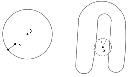
Based on the definition, the reach $\tau_{\iota(M)}$ of $\iota(M)$ is the largest number such that any point in $\mathbb{R}^{D}$ at distance less than the reach from $\iota(M)$ has a unique nearest point on $\iota(M)$. The reaches of some special embedded submanifolds can be explicitly calculated. For example, the reach of a $d$ dimensional round sphere in $\mathbb{R}^{D}$ is the radius of the sphere. We have the following topological result about the reach of $\iota(M)$. A consequence of the result says that if we can find a point $\textbf{y}\in\mathbb{R}^{D}$ and a radius $\xi$ such that $B^{\mathbb{R}^{D}}_{\xi}(\textbf{y})\cap\iota(M)$ has more than one connected component, then $\tau_{\iota(M)}<\xi$. In Figure 4, we illustrate the concept of reach by using this consequence.

Figure 4. Left panel: The reach of a circle in the plane is the radius. For the center of the circle, the nearest point on the circle is the whole circle. For any point y whose distance to the circle is less than the radius, there is a unique nearest point on the circle. Right panel: A closed curve in the plane with small reach. We can find a point y and a small ball of radius $r$ centered at y. The intersection between the ball and the curve has two connected components. Hence, by the consequence of Proposition 1, the reach of the curve is smaller than $r$.

Proposition 1 (Proposition 1 [4]).

Suppose $0<\xi<\tau_{\iota(M)}$. For any $\textbf{y}\in\mathbb{R}^{D}$, If $B^{\mathbb{R}^{D}}_{\xi}(\textbf{y})\cap\iota(M)\not=\emptyset$, then $B^{\mathbb{R}^{D}}_{\xi}(\textbf{y})\cap\iota(M)$ is an open subset of $\iota(M)$ that is homeomorphic to $B^{\mathbb{R}^{d}}_{1}(0)$.

As we introduced previously, for any $x\in M$, there is a chart of $\iota(M)$ over a neighborhood $U_{x}\cap\iota(M)\subset\mathbb{R}^{D}$ around $\iota(x)$. However, the size of $U_{x}$ may not be uniform for all $x$. In the next proposition, by applying Proposition 1, we show that we can choose the neighborhoods $\{U_{x}\}$ to be uniform for all $x$. In particular, we can construct a chart over $B^{\mathbb{R}^{D}}_{\xi}(\iota(x))\cap\iota(M)$ for any $\xi<\frac{\tau_{\iota(M)}}{2}$. The proposition will be used later in the proof of the main theorem. The proof of the proposition is in Appendix C.

Proposition 2.

Suppose $0<\xi<\frac{\tau_{\iota(M)}}{2}$. For any $x\in M$, there is an open set $V_{x}\subset B^{\mathbb{R}^{d}}_{\xi}(0)\subset\mathbb{R}^{d}$ containing $0$ such that for any $\textbf{y}\in B^{\mathbb{R}^{D}}_{\xi}(\iota(x))\cap\iota(M)$, we have

$$\textbf{y}=\iota(x)+X(x)\begin{bmatrix}\textbf{u}\\ G_{x}(\textbf{u})\end{bmatrix},$$

where $\textbf{u}\in V_{x}$. Moreover,

1. $\{Xe_{i}\}_{i=1}^{d}$ form a basis of $\iota_{*}T_{x}M$.

2. $V_{x}$ is homeomorphic to $B^{\mathbb{R}^{d}}_{1}(0)$.

3. $G_{x}(\textbf{u})=[g_{x,1}(\textbf{u}),\cdots,g_{x,D-d}(\textbf{u})]^{\top}\in\mathbb{R}^{D-d}$ and each $g_{x,i}$ is a smooth function on $V_{x}$.

4. $g_{x,i}(0)=0$ and $\mathcal{D}g_{x,i}(0)=0$ for $i=1,\cdots,D-d$, where $\mathcal{D}g_{x,i}$ is the derivative of $g_{x,i}$.

This proposition uses the fact that the projection of $\textbf{y}-\iota(x)$ onto the tangent space $\iota_{*}T_{x}M$ is a diffeomorphism for $\textbf{y}\in B^{\mathbb{R}^{D}}_{\xi}(\iota(x))\cap\iota(M)$. Hence, it can be used to construct a chart for $\iota(M)$.

3.2. Local covariance matrix on manifold with noise

Recall Assumption 1, and let $G_{\sigma}(\eta)$ denote the $\mathcal{N}(0,\sigma^{2}I_{D\times D})$ probability density function of $\eta$. Since the samples $\{\eta_{1}\cdots,\eta_{n}\}$ are independent of $\{x_{1}\cdots,x_{n}\}$, the pairs $\{(x_{i},\eta_{i})\}_{i=1}^{n}$ can be regarded as $n$ i.i.d samples based on the probability density function $P(x)G_{\sigma}(\eta)$ on $M\times\mathbb{R}^{D}$.

Note that $C_{n,\epsilon}(\textbf{y}_{k})$ is invariant under the translation of $\iota(M)$ in $\mathbb{R}^{D}$. Hence, to simplify the notation, for any fixed $x_{k}\in M$, we translate $\iota(M)$ and apply an orthogonal transformation in $\mathbb{R}^{D}$ so that $\iota(x_{k})=0\in\mathbb{R}^{D}$ and $\{e_{i}\}_{i=1}^{d}$ form a basis of $\iota_{*}T_{x_{k}}M$. Suppose $\mathbb{X}$ is a random variable associated with the probability density function $P(x)$ on $M$. Suppose $\mathbb{H}$ is a random variable associated with the probability density function $G_{\sigma}(\eta)$ on $\mathbb{R}^{D}$. Since $\iota(x_{k})=0$, we have $\textbf{y}_{k}=\iota(x_{k})+\eta_{k}=\eta_{k}$. Based on the above setup, the expectation of the local covariance matrix at $\textbf{y}_{k}$ is defined as follows:

(14) $$C_{\epsilon}(\textbf{y}_{k}):= \mathbb{E}\Big{[}(\iota(\mathbb{X})+\mathbb{H}-\eta_{k})(\iota(\mathbb{X})+\mathbb{H}-\eta_{k})^{\top}\chi\big{(}\frac{\|\iota(\mathbb{X})+\mathbb{H}-\eta_{k}\|_{\mathbb{R}^{D}}}{\epsilon}\big{)}\Big{]}$$

$$= \int_{\mathbb{R}^{D}}\int_{M}(\iota(x)+\eta-\eta_{k})(\iota(x)+\eta-\eta_{k})^{\top}\chi\big{(}\frac{\|\iota(x)+\eta-\eta_{k}\|_{\mathbb{R}^{D}}}{\epsilon}\big{)}P(x)G_{\sigma}(\eta)dVd\eta.$$

Remark 1.

Suppose $f:\mathbb{R}^{D}\rightarrow\mathbb{R}$ is a measurable function. Then, by change of variables, we have

$$\int_{\mathbb{R}^{D}}\int_{M}f(\iota(x)+\eta)P(x)G_{\sigma}(\eta)dVd\eta= \int_{\mathbb{R}^{D}}\int_{M}f(\eta)P(x)G_{\sigma}(\eta-\iota(x))dVd\eta$$

$$= \int_{\mathbb{R}^{D}}f(\eta)P\star G_{\sigma}(\eta)d\eta,$$

where the convolution $P\star G_{\sigma}(\eta):=\int_{M}P(x)G_{\sigma}(\eta-\iota(x))dV$ is the probability density function for the random variable $\iota(\mathbb{X})+\mathbb{H}$. Hence, the definition in (14) is equivalent to

(15) $$\mathbb{E}[(\iota(\mathbb{X})+\mathbb{H}-\eta_{k})(\iota(\mathbb{X})+\mathbb{H}-\eta_{k})^{\top}\chi(\frac{\|\iota(\mathbb{X})+\mathbb{H}-\eta_{k}\|_{\mathbb{R}^{D}}}{\epsilon})]$$

$$= \int_{\mathbb{R}^{D}}(\eta-\eta_{k})(\eta-\eta_{k})^{\top}\chi(\frac{\|\eta-\eta_{k}\|_{\mathbb{R}^{D}}}{\epsilon})P\star G_{\sigma}(\eta)d\eta.$$

In the following proposition, we provide a bias analysis for the local covariance matrix. The proof of the proposition is in Appendix A.

Proposition 3.

Under Assumption 1, suppose $\epsilon$ is small enough depending on $d$, $D$, the second fundamental form of $\iota(M)$ and the scalar curvature of $M$. For any $\alpha>\frac{3}{2}$, suppose $1<\beta\leq\alpha-\frac{1}{2}$. If $\sigma=\epsilon^{\alpha}$ and $\|\eta_{k}\|_{\mathbb{R}^{D}}\leq\epsilon^{\beta}$, then

$$C_{\epsilon}(\textbf{y}_{k})=\epsilon^{d+2}\Bigg{(}\frac{|S^{d-1}|{P}(x_{k})}{d(d+2)}\begin{bmatrix}I_{d\times d}&0\\ 0&0\\ \end{bmatrix}+\begin{bmatrix}O(\epsilon^{\beta-1}+\epsilon^{2})&O(\epsilon^{2\beta-2}+\epsilon^{2})\\ O(\epsilon^{2\beta-2}+\epsilon^{2})&O(\epsilon^{2\beta-2}+\epsilon^{2})\end{bmatrix}\Bigg{)},$$

where the constant factors in all blocks depend on $d$, $C^{2}$ norm of $P$, the second fundamental form of $\iota(M)$ and its derivative and the Ricci curvature of $M$.

Supposing $\iota(x_{k})=0$ and there is no noise, then the expectation of the local covariance matrix at $\textbf{y}_{k}$ can be expressed as follows:

$$\tilde{C}_{\epsilon}(\textbf{y}_{k})=\mathbb{E}[\iota(\mathbb{X})\iota(\mathbb{X})^{\top}\chi(\frac{\|\iota(\mathbb{X})\|_{\mathbb{R}^{D}}}{\epsilon})].$$

By Proposition 3.1 in [33],

$$\tilde{C}_{\epsilon}(\textbf{y}_{k})=\epsilon^{d+2}\Bigg{(}\frac{|S^{d-1}|{P}(x_{k})}{d(d+2)}\begin{bmatrix}I_{d\times d}&0\\ 0&0\\ \end{bmatrix}+O(\epsilon^{2})\Bigg{)},$$

where $O(\epsilon^{2})$ represents a $D$ by $D$ matrix whose entries are of order $O(\epsilon^{2})$. The constant factors in $O(\epsilon^{2})$ depend on $d$, $C^{2}$ norm of $P$, the second fundamental form of $\iota(M)$ and its derivative and the Ricci curvature of $M$. If the variance of the Gaussian noise is small enough, so that $\sigma^{2}=\epsilon^{2\alpha}$ with $\alpha\geq\frac{7}{2}$, and suppose we can choose $\beta\geq 3$, then

$$C_{\epsilon}(\textbf{y}_{k})=\epsilon^{d+2}\Bigg{(}\frac{|S^{d-1}|{P}(x_{k})}{d(d+2)}\begin{bmatrix}I_{d\times d}&0\\ 0&0\\ \end{bmatrix}+O(\epsilon^{2})\Bigg{)}.$$

Comparing to Proposition 3.1 in [33], we conclude that the impact of the noise on the local covariance matrix is negligible in this case. In the next proposition, we provide a variance analysis of the local covariance matrix. The proof is in Appendix B.

Proposition 4.

Under Assumption 1, suppose $\epsilon$ is small enough depending on $d$, $D$, the second fundamental form of $\iota(M)$ and the scalar curvature of $M$. Suppose $\sigma=\epsilon^{\alpha}$ for $\alpha>\frac{3}{2}$. If $n\leq\frac{1}{2}\exp(\frac{1}{12\epsilon^{2(\alpha-\beta)}})$ for some $\beta$ such that $1<\beta\leq\alpha-\frac{1}{2}$, then for all $x_{k}$, with probability greater than $1-\frac{1}{n^{2}}$, we have $\|\eta_{k}\|_{\mathbb{R}^{D}}\leq\epsilon^{\beta}$, and

(16) $$C_{n,\epsilon}(\textbf{y}_{k})=\epsilon^{d+2}\Bigg{(}\frac{|S^{d-1}|{P}(x_{k})}{d(d+2)}\begin{bmatrix}I_{d\times d}&0\\ 0&0\\ \end{bmatrix}+\mathcal{E}\Bigg{)},$$

where

$$\mathcal{E}=\begin{bmatrix}O(\epsilon^{\min(\beta-1,2)}+\sqrt{\frac{\log n}{n\epsilon^{d}}})&O(\epsilon^{2\min(\beta-1,1)}+\sqrt{\frac{\log n}{n\epsilon^{d-2\min(\beta-1,1)}}})\\ O(\epsilon^{2\min(\beta-1,1)}+\sqrt{\frac{\log n}{n\epsilon^{d-2\min(\beta-1,1)}}})&O(\epsilon^{2\min(\beta-1,1)}+\sqrt{\frac{\log n}{n\epsilon^{d-2\min(\beta-1,1)}}})\end{bmatrix}.$$

The top left block of $\mathcal{E}$ is a $d$ by $d$ matrix. The constant factors in $\mathcal{E}$ depend on $d$, $C^{2}$ norm of $P$, the second fundamental form of $\iota(M)$ and its derivative and the Ricci curvature of $M$.

The following proposition describes the structure of the orthonormal eigenvector matrix of $C_{n,\epsilon}(\textbf{y}_{k})$ from (2). The proof relies on applying the Davis-Kahan theorem to Proposition 4. In order to acquire a large enough lower bound on the eigengap between the $d$th eigenvalue and the $(d+1)$th eigenvalue of $C_{n,\epsilon}(\textbf{y}_{k})$, we need the variance of the Gaussian noise to be smaller than the requirement in Proposition 4, e.g. $\sigma^{2}=\epsilon^{2\alpha}$ with $\alpha\geq\frac{7}{4}$ rather than $\alpha>\frac{3}{2}$. The proof of the proposition is in Appendix B.

Proposition 5.

Under Assumption 1, suppose $\epsilon$ is small enough depending on $d$, $D$, $P_{m}$, $C^{2}$ norm of $P$, the second fundamental form of $\iota(M)$ and its derivative and the Ricci curvature of $M$. Suppose $\sigma=\epsilon^{\alpha}$ for $\alpha\geq\frac{7}{4}$. If $\epsilon^{-d-2\min(\beta-1,1)}\leq\frac{n}{\log n}$ and $n\leq\frac{1}{2}\exp(\frac{1}{12\epsilon^{2(\alpha-\beta)}})$ for some $\beta$ such that $\frac{5}{4}\leq\beta\leq\alpha-\frac{1}{2}$, then for all $x_{k}$, with probability greater than $1-\frac{1}{n^{2}}$, we have $\|\eta_{k}\|_{\mathbb{R}^{D}}\leq\epsilon^{\beta}$, and

(17) $$U_{n,\epsilon}(\textbf{y}_{k})=\begin{bmatrix}X_{1}&0\\ 0&X_{2}\\ \end{bmatrix}+O(\epsilon^{2\min(\beta-1,1)}),$$

where $X_{1}\in\mathbb{O}(d)$, $X_{2}\in\mathbb{O}(D-d)$. $O(\epsilon^{2\min(\beta-1,1)})$ represents a $D$ by $D$ matrix whose entries are of order $O(\epsilon^{2\min(\beta-1,1)})$, where the constant factors depend on $d$, $D$, $P_{m}$, $C^{2}$ norm of $P$, the second fundamental form of $\iota(M)$ and its derivative and the Ricci curvature of $M$.

Proposition 5 depends on lower and upper bounds on the sample size $n$. We first discuss the lower bound for $n$. If there exists $\beta$ with $\frac{5}{4}\leq\beta$ such that $\epsilon^{-d-2\min(\beta-1,1)}\leq\frac{n}{\log n}$, then $n$ should not be too small and should satisfy $\frac{n}{\log n}\geq\epsilon^{-d-\frac{1}{2}}$. Intuitively, since $\{x_{i}\}_{i=1}^{n}$ are sampled based on a p.d.f having a positive lower bound, to achieve a large enough eigengap between the $d$th and $(d+1)$th eigenvalue of $C_{n,\epsilon}(\textbf{y}_{k})$, $n$ should be large enough so that there are enough samples in any $\epsilon$ geodesic ball on the manifold. The upper bound on $n$ implies a relation between $n$ and $\sigma$. To achieve $n\leq\frac{1}{2}\exp(\frac{1}{12\epsilon^{2(\alpha-\beta)}})$, $n$ should not exceed $\frac{1}{2}\exp(\frac{1}{12\epsilon^{2\alpha-\frac{5}{2}}})$. Intuitively, since $\{\eta_{i}\}$ are Gaussian noise, if $n$ is too large, then there will be more $\eta_{i}$ with large magnitude. As $C_{n,\epsilon}(\textbf{y}_{k})$ is the covariance matrix for local PCA, there will be more than $d$ principal components in an $\epsilon$ Euclidean ball around $\textbf{y}_{k}$. Hence, there will be a significant difference between the subspace generated by eigenvectors corresponding to the first $d$ eigenvalues of $C_{n,\epsilon}(\textbf{y}_{k})$ and $\iota_{*}T_{x_{k}}M$. On the other hand, if there is $\beta$ such that $n\leq\frac{1}{2}\exp(\frac{1}{12\epsilon^{2(\alpha-\beta)}})$ holds, then $\sigma^{2}\leq\frac{\epsilon^{\beta}}{12\log(2n)}\leq\frac{\epsilon^{\frac{5}{4}}}{12\log(2n)}$. Asymptotically, since $\alpha-\beta\geq\frac{1}{2}$, $n\leq\frac{1}{2}\exp(\frac{1}{12\epsilon^{2(\alpha-\beta)}})$ implies $\epsilon\rightarrow 0$ as $n\rightarrow\infty$. Hence, as $\sigma=\epsilon^{\alpha}$ with $\alpha\geq\frac{7}{4}$, we have $\sigma\rightarrow 0$ as $n\rightarrow\infty$.

If $n$ satisfies the requirements in Proposition 5 so that there is $\beta$ with $\frac{5}{4}\leq\beta\leq\alpha-\frac{1}{2}$, then

(18) $$U_{n,\epsilon}(\textbf{y}_{k})-\begin{bmatrix}X_{1}&0\\ 0&X_{2}\\ \end{bmatrix}=O(\epsilon^{2\min(\beta-1,1)}).$$

Since $\frac{5}{4}\leq\beta$, $O(\epsilon^{2\min(\beta-1,1)})$ should be at most order $\epsilon^{\frac{1}{2}}$. In our algorithm, we use the first $d$ column vectors of $U_{n,\epsilon}(\textbf{y}_{k})$ to construct a projection map $\mathcal{P}_{\textbf{y}_{k}}(\textbf{y})$ from $\mathbb{R}^{D}$ to $\mathbb{R}^{d}$ defined in (3). We will show that when we restrict the map $\mathcal{P}_{\textbf{y}_{k}}(\textbf{y})$ on $\iota(M)$, it is not necessary that the entries of $U_{n,\epsilon}(\textbf{y}_{k})-\begin{bmatrix}X_{1}&0\\ 0&X_{2}\\ \end{bmatrix}$ are very small for the map to be a local diffeomorphism.

3.3. Construction of a chart from noisy samples

In this subsection, we will show that the projection map $\mathcal{P}_{\textbf{y}_{k}}(\textbf{y})$ defined in (3) is a local diffeomorphism on $\iota(M)$ and its inverse is a chart of $\iota(M)$. We first define a projection map from $\mathbb{R}^{D}$ to $\mathbb{R}^{d}$. This generalizes the projection map in (3).

Definition 2.

Fix $x\in M$. Suppose $U\in\mathbb{O}(D)$. For any vector $\textbf{a}\in\mathbb{R}^{D}$, we define a projection map for $\textbf{y}\in\mathbb{R}^{D}$ to the subspace generated by the first $d$ column vectors of $U$:

$$\mathcal{P}_{U,\iota(x)+\textbf{a}}(\textbf{y})=J^{\top}U^{\top}(\textbf{y}-\iota(x)-\textbf{a}).$$

We show that, under suitable conditions on a and $U$, the above projection is a local diffeomorphism when it is restricted on $\iota(M)$. For any $x\in M$, if we have a $d$ dimension subspace of $\mathbb{R}^{D}$ which does not deviate too far away from the tangent space $\iota_{*}T_{x}M$, then for any point $\iota(x)+\textbf{a}\in\mathbb{R}^{D}$ that is not too far away from $\iota(x)$ and any y around $\iota(x)+\textbf{a}$ on $\iota(M)$, the projection of $\textbf{y}-\iota(x)-\textbf{a}$ onto the subspace is a diffeomorphism. Hence, we can use the projection to construct a chart. Our next proposition formalizes this argument. The proof is in Appendix C.

Before we state the proposition. We make the following observation. For any $\textbf{y}\in\iota(M)$, the map $\mathcal{P}_{U,\iota(x)+\textbf{a}}(\textbf{y})$ is invariant under translations of the manifold in $\mathbb{R}^{D}$: for any b, we have

$$\mathcal{P}_{U,\iota(x)+\textbf{a}}(\textbf{y})=J^{\top}U^{\top}(\textbf{y}-\iota(x)-\textbf{a})=J^{\top}U^{\top}(\textbf{y}+\textbf{b}-(\iota(x)+\textbf{b})-\textbf{a})^{\top}.$$

Moreover, $\mathcal{P}_{U,\iota(x)+\textbf{a}}(\textbf{y})$ is invariant under an orthogonal transformation in $\mathbb{R}^{D}$: for any $V\in\mathbb{O}(D)$,

$$\mathcal{P}_{U,\iota(x)+\textbf{a}}(\textbf{y})=J^{\top}U^{\top}(\textbf{y}-\iota(x)-\textbf{a})=J^{\top}U^{\top}V^{\top}V(\textbf{y}-\iota(x)-\textbf{a}).$$

Hence, when we discuss the map $\mathcal{P}_{U,\iota(x)+\textbf{a}}(\textbf{y})$, we can always translate $\iota(M)$ and apply an orthogonal transformation in $\mathbb{R}^{D}$ so that that $\iota(x)=0\in\mathbb{R}^{D}$ and $\iota_{*}T_{x}M$ is generated by $\{e_{i}\}_{i=1}^{d}$.

Proposition 6.

For $x\in M$, suppose we translate $\iota(M)$ and apply an orthogonal transformation in $\mathbb{R}^{D}$ so that $\iota(x)=0\in\mathbb{R}^{D}$ and $\{Xe_{i}\}_{i=1}^{d}$ form a basis of $\iota_{*}T_{x}M$ where $X=\begin{bmatrix}X_{1}&0\\ 0&X_{2}\\ \end{bmatrix}\in\mathbb{O}(D)$ with $X_{1}\in\mathbb{O}(d)$ and $X_{2}\in\mathbb{O}(D-d)$. Suppose $U\in\mathbb{O}(D)$ and $E=U-X$ with $|E_{ij}|<r$. For any $0<\xi\leq\frac{2\tau_{\iota(M)}}{9}$ and $r\leq\frac{1}{6d^{\frac{3}{2}}}$, if $\|\textbf{a}\|_{\mathbb{R}^{D}}<\frac{\xi}{2}$, then we have the following facts:

1. $\mathcal{P}_{U,\iota(x)+\textbf{a}}$ is a diffeomorphism from $B^{\mathbb{R}^{D}}_{\xi}(\iota(x)+\textbf{a})\cap\iota(M)$ onto its image $O\subset\mathbb{R}^{d}$. $O$ is homeomorphic to $B^{\mathbb{R}^{d}}_{1}(0)$.

2. There is a point $\textbf{u}_{0}$ in $O$ such that $B^{\mathbb{R}^{d}}_{R}(\textbf{u}_{0})\subset O\subset B^{\mathbb{R}^{d}}_{\xi}(0)$. Let $A=1-d^{\frac{3}{2}}r$ and $B=\frac{2(\xi+\|\textbf{a}\|_{\mathbb{R}^{D}})}{\tau_{\iota(M)}}$. Then $R\geq(\sqrt{A^{2}-A^{2}B}-\sqrt{B-A^{2}B})(\xi-\|\textbf{a}\|_{\mathbb{R}^{D}})$.

Recall the projections that we defined in (3) and (4). In the following theorem, we show that, with high probability, $\mathcal{P}_{\textbf{y}_{k}}(\textbf{y})$ is a diffeomorphism from $B^{\mathbb{R}^{D}}_{2\delta}(\textbf{y}_{k})\cap\iota(M)$ onto its image for some $\delta>0$. Note that $\mathcal{P}_{\textbf{y}_{k}}(\textbf{y})=\mathcal{P}_{U_{n,\epsilon},\iota(x_{k})+\eta_{k}}(\textbf{y})$, hence the proof of the theorem in Appendix C is a combination of Proposition 5 and Proposition 6.

Theorem 1.

Under Assumption 1, suppose $\epsilon$ is small enough depending on $d$, $D$, $P_{m}$, $C^{2}$ norm of $P$, the second fundamental form of $\iota(M)$ and its derivative and the Ricci curvature of $M$. Moreover, $\epsilon<\frac{\tau_{\iota(M)}}{9}$. Suppose $\sigma=\epsilon^{\alpha}$ for $\alpha\geq\frac{7}{4}$. If $\epsilon^{-d-2\min(\beta-1,1)}\leq\frac{n}{\log n}$ and $n\leq\frac{1}{2}\exp(\frac{1}{12\epsilon^{2(\alpha-\beta)}})$ for some $\beta$ such that $\frac{5}{4}\leq\beta\leq\alpha-\frac{1}{2}$, then for all $x_{k}$ and any $\delta$ such that $\epsilon^{\beta}<\delta<\frac{\tau_{\iota(M)}}{9}$, with probability greater than $1-\frac{1}{n^{2}}$, we have the following facts:

1. If $\textbf{y}_{i}\in B^{\mathbb{R}^{D}}_{\delta}(\textbf{y}_{k})$, then $\iota(x_{i})\in B^{\mathbb{R}^{D}}_{2\delta}(\textbf{y}_{k})$.

2. The map $\mathcal{P}_{\textbf{y}_{k}}(\textbf{y})$ defined in (3) is a diffeomorphism from $B^{\mathbb{R}^{D}}_{2\delta}(\textbf{y}_{k})\cap\iota(M)$ onto its image $O_{k}\subset\mathbb{R^{d}}$. $O_{k}$ is homeomorphic to $B^{\mathbb{R}^{d}}_{1}(0)$.

3. There is a point $\textbf{u}_{k,0}$ in $O_{k}$ such that $B^{\mathbb{R}^{d}}_{R_{k}}(\textbf{u}_{k,0})\subset O_{k}\subset B^{\mathbb{R}^{d}}_{2\delta}(0)$. Let $A=1-\Omega\epsilon^{2\min(\beta-1,1)}$ and $B=\frac{4\delta+2\epsilon^{\beta}}{\tau_{\iota(M)}}$, where $\Omega$ is a constant depending on $d$, $D$, $P_{m}$, $C^{2}$ norm of $P$, the second fundamental form of $\iota(M)$ and its derivative and the Ricci curvature of $M$. Then

   $$R_{k}\geq(\sqrt{A^{2}-A^{2}B}-\sqrt{B-A^{2}B})(2\delta-\epsilon^{\beta}).$$

We discuss the set $O_{k}$ in the above theorem. Depending on the variance of the noise, the last part of the theorem describes how close to round $O_{k}$ is. First consider the extreme case when there is no noise. Equivalently, we can take $\alpha\rightarrow\infty$ and $\beta=\frac{\alpha}{2}\rightarrow\infty$, then the relations $\epsilon^{-d-2\min(\beta-1,1)}\leq\frac{n}{\log n}$ and $n\leq\frac{1}{2}\exp(\frac{1}{12\epsilon^{2(\alpha-\beta)}})$ are satisfied when the sample size $n$ satisfies $\epsilon^{-d-2}\leq\frac{n}{\log n}$. By a straightforward calculation, if $\epsilon$ and $\delta$ satisfy the conditions in the theorem, then $R_{k}\geq 2(1-\frac{4\delta}{\tau_{\iota(M)}}-\Omega^{\prime}\epsilon)\delta$, for some constant $\Omega^{\prime}$ depending on $\Omega$. Hence, $O_{k}$ is close to round in the sense that $O_{k}$ is contained in the round ball of radius $2\delta$ and it contains a round ball of radius close to $2\delta$. In general, when $\sigma$ is small, then $\alpha$ is large and we can choose $\beta$ to be large so that for given $n$, the relations $\epsilon^{-d-2\min(\beta-1,1)}\leq\frac{n}{\log n}$ and $n\leq\frac{1}{2}\exp(\frac{1}{12\epsilon^{2(\alpha-\beta)}})$ are satisfied. In this case, $R_{k}$ is closer to $2\delta$. Consequently, when the samples are less noisy, the set $O_{k}$ becomes more regular in the sense that it is always contained in $B^{\mathbb{R}^{d}}_{2\delta}(0)$ and it contains a round ball with radius closer to $2\delta$.

In conclusion, based on Theorem 1, if $\epsilon$, $\delta$, $\sigma$ and $n$ satisfy the conditions, then the inverse of the map $\mathcal{P}_{\textbf{y}_{k}}(\textbf{y})$ from $O_{k}$ to $B^{\mathbb{R}^{D}}_{2\delta}(\textbf{y}_{k})\cap\iota(M)$ is a chart of $\iota(M)$. Moreover, for all $\textbf{y}_{i}\in B^{\mathbb{R}^{D}}_{\delta}(\textbf{y}_{k})$, the corresponding $\iota(x_{i})$ is in the image of the chart. When $\sigma$ is smaller, the domain $O_{k}$ becomes more regular. In the following subsections, we will discuss how to use $\{\mathcal{P}_{\textbf{y}_{k}}(\textbf{y}_{i})\}$ and $\{\mathcal{P}^{\bot}_{\textbf{y}_{k}}(\textbf{y}_{i})\}$ for $\textbf{y}_{i}\in B^{\mathbb{R}^{D}}_{\delta}(\textbf{y}_{k})$ to recover information about the inverse of the map $\mathcal{P}_{\textbf{y}_{k}}(\textbf{y})$.

3.4. Setup of the regression functions

We describe a chart of $\iota(M)$ around $\iota(x_{k})$ and an associated regression problem implied by Theorem 1. Suppose $\epsilon$, $\delta$, $\sigma$ and $n$ satisfy the conditions in Theorem 1. Then, all the following statements hold with probability greater than $1-\frac{1}{n^{2}}$. If the image of $B^{\mathbb{R}^{D}}_{2\delta}(\textbf{y}_{k})\cap\iota(M)$ under $\mathcal{P}_{\textbf{y}_{k}}(\textbf{y})$ is $O_{k}\subset\mathbb{R}^{d}$, then $\mathcal{P}_{\textbf{y}_{k}}(\textbf{y})$ is a diffeomorphism from $B^{\mathbb{R}^{D}}_{2\delta}(\textbf{y}_{k})\cap\iota(M)$ to $O_{k}$. $O_{k}$ is an open set in $\mathbb{R}^{d}$ homeomorphic to $B^{\mathbb{R}^{d}}_{1}(0)$. If $\Phi_{k}$ is the inverse of $\mathcal{P}_{\textbf{y}_{k}}(\textbf{y})$ from $O_{k}$ to $B^{\mathbb{R}^{D}}_{2\delta}(\textbf{y}_{k})\cap\iota(M)$, then $\Phi_{k}$ is a chart of $\iota(M)$. Based on (3),

(19) $$\Phi_{k}(\textbf{u})=\textbf{y}_{k}+U_{n,\epsilon}(\textbf{y}_{k})\begin{bmatrix}\textbf{u}\\ F_{k}(\textbf{u}),\\ \end{bmatrix}$$

where $F_{k}(\textbf{u}):O_{k}\rightarrow\mathbb{R}^{D-d}$ is a smooth function. Note that

(20) $$F_{k}(\textbf{u})=\mathcal{P}^{\bot}_{\textbf{y}_{k}}(\Phi_{k}(\textbf{u})).$$

Let $\eta_{i,1}=J^{\top}U_{n,\epsilon}(\textbf{y}_{k})^{\top}\eta_{i}\in\mathbb{R}^{d}$ and $\eta_{i,2}=\bar{J}^{\top}U_{n,\epsilon}(\textbf{y}_{k})^{\top}\eta_{i}\in\mathbb{R}^{D-d}$. Suppose $B^{\mathbb{R}^{D}}_{\delta}(\textbf{y}_{k})\cap\{\textbf{y}_{1},\cdots,\textbf{y}_{n}\}=\{\textbf{y}_{k,1},\cdots,\textbf{y}_{k,N_{k}}\}$. By Theorem 1, we have $\iota(x_{k,i})\in B^{\mathbb{R}^{D}}_{2\delta}(\textbf{y}_{k})$ for $i=1,\cdots,N_{k}$. Hence,

$$\textbf{u}_{k,i}=\mathcal{P}_{\textbf{y}_{k}}(\iota(x_{k,i})),\quad\quad\iota(x_{k,i})=\Phi_{k}(\textbf{u}_{k,i}),$$

$$\textbf{y}_{k,i}=\iota(x_{k,i})+\eta_{k,i}=\Phi_{k}(\textbf{u}_{k,i})+\eta_{k,i},$$

with $\textbf{u}_{k,i}\in O_{k}$. Moreover,

(21) $$\mathcal{P}_{\textbf{y}_{k}}(\textbf{y}_{k,i})= J^{\top}U_{n,\epsilon}(\textbf{y}_{k})^{\top}(\iota(x_{k,i})+\eta_{k,i}-\iota(x_{k})-\eta_{k})$$

$$= J^{\top}U_{n,\epsilon}(\textbf{y}_{k})^{\top}(\iota(x_{k,i})-\iota(x_{k})-\eta_{k})+J^{\top}U_{n,\epsilon}(\textbf{y}_{k})^{\top}\eta_{k,i}$$

$$= \textbf{u}_{k,i}+\eta_{k,i,1}.$$

(22) $$\mathcal{P}^{\bot}_{\textbf{y}_{k}}(\textbf{y}_{k,i})= \bar{J}^{\top}U_{n,\epsilon}(\textbf{y}_{k})^{\top}(\iota(x_{k,i})+\eta_{k,i}-\iota(x_{k})-\eta_{k})$$

$$= \bar{J}^{\top}U_{n,\epsilon}(\textbf{y}_{k})^{\top}(\iota(x_{k,i})-\iota(x_{k})-\eta_{k})+\bar{J}^{\top}U_{n,\epsilon}(\textbf{y}_{k})^{\top}\eta_{k,i}$$

$$= \mathcal{P}^{\bot}_{\textbf{y}_{k}}(\Phi_{k}(\textbf{u}_{k,i}))+\bar{J}^{\top}U_{n,\epsilon}(\textbf{y}_{k})^{\top}\eta_{k,i}$$

$$= F_{k}(\textbf{u}_{k,i})+\eta_{k,i,2}.$$

If we can recover the function $F_{k}$ by using the pairs $\big{(}\mathcal{P}_{\textbf{y}_{k}}(\textbf{y}_{k,i}),\mathcal{P}^{\bot}_{\textbf{y}_{k}}(\textbf{y}_{k,i})\big{)}_{i=1}^{N_{k}}$, then, for $\textbf{u}\in O_{k}$, (19) provides a point in $B^{\mathbb{R}^{D}}_{2\delta}(\textbf{y}_{k})\cap\iota(M)$. Therefore, we introduce the following errors-in-variables regression problem. Suppose $F=(f_{1},\cdots,f_{p}):O\subset\mathbb{R}^{d}\rightarrow\mathbb{R}^{q}$, with $q=D-d$, is an unknown regression function, where $O$ is an unknown open subset homeomorphic to a $d$ dimensional open ball in $\mathbb{R}^{d}$. We observe the labeled training data $(\textbf{w}_{i},\textbf{z}_{i})_{i=1}^{N}$, where

(23) $$\textbf{w}_{i}=\textbf{u}_{i}+\eta_{i,1}, \eta_{i,1}\sim\mathcal{N}(0,\sigma^{2}I_{d\times d}),$$

$$\textbf{z}_{i}=F(\textbf{u}_{i})+\eta_{i,2}, \eta_{i,2}\sim\mathcal{N}(0,\sigma^{2}I_{q\times q}),$$

and $\{\textbf{u}_{i}\}_{i=1}^{N}\subset O$. The goal is to predict $F(\textbf{u})$ for $\textbf{u}\in O$.

3.5. Discussion of the main algorithm

In this subsection, by applying the previous theoretical results, we provide a discussion of the main algorithms. First, we choose $\epsilon$ so that each $B^{\mathbb{R}^{D}}_{\epsilon}(\textbf{y}_{k})\cap\{\textbf{y}_{1},\cdots,\textbf{y}_{n}\}$ has more than $d$ points. Hence, for each $k$, we can find the eigenvectors corresponding to the largest $d$ eigenvalues of $C_{n,\epsilon}(\textbf{y}_{k})$. We choose $\delta>\epsilon$ to satisfy the requirement of Theorem 1.

Step 1 of Algorithm 1: Setup of the predictors and the response variables for charts of $\iota(M)$. For each $k$, we find all the samples $\{\textbf{y}_{j}\}$ in $B^{\mathbb{R}^{D}}_{\delta}(\textbf{y}_{k})$. Suppose there are $N_{k}$ samples in $B^{\mathbb{R}^{D}}_{\delta}(\textbf{y}_{k})$, denoted $\{\textbf{y}_{k,1},\cdots,\textbf{y}_{k,N_{k}}\}$. Denote $\textbf{w}_{k,j}=\mathcal{P}_{\textbf{y}_{k}}(\textbf{y}_{k,j})$ and $\textbf{z}_{k,j}=\mathcal{P}^{\bot}_{\textbf{y}_{k}}(\textbf{y}_{k,j})$ for $j=1,\cdots,N_{k}$. Observe that $\mathcal{P}_{\textbf{y}_{k}}(\textbf{y}_{k})=0$. Then, by (21) and (22), we have

(24) $$\textbf{w}_{k,j}=\textbf{u}_{k,j}+\eta_{k,j,1} \eta_{k,j,1}\sim\mathcal{N}(0,\sigma^{2}I_{d\times d}),$$

$$\textbf{z}_{k,j}=F_{k}(\textbf{u}_{k,j})+\eta_{k,j,2} \eta_{k,j,2}\sim\mathcal{N}(0,\sigma^{2}I_{(D-d)\times(D-d)}),$$

where $F_{k}:O_{k}\subset\mathbb{R}^{d}\rightarrow\mathbb{R}^{D-d}$ is described in (20). $O_{k}$ is homeomorphic to a $d$ dimensional open ball. $\{\textbf{u}_{k,j}\}_{j=1}^{N_{k}}$ are in $O_{k}$. The map $\Phi_{k}:O_{k}\rightarrow B^{\mathbb{R}^{D}}_{2\delta}(\textbf{y}_{k})\cap\iota(M)$ described in (19) is a chart of $\iota(M)$ containing $\iota(x_{k})$. Our goal is to reconstruct the chart so that we can predict

$$\textbf{y}_{k}+U_{n,\epsilon}(\textbf{y}_{k})\begin{bmatrix}0\\ F_{k}(0)\\ \end{bmatrix}.$$

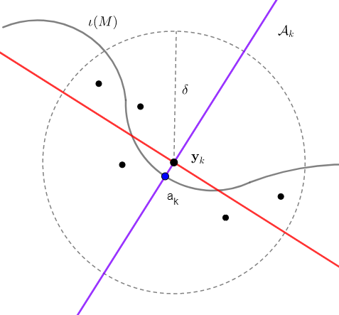
Predictive distribution of the initial denoised samples (from Steps 2 to 3). We solve $F_{k}(0)$ by applying GP regression to (24) , while ignoring the errors of $\textbf{w}_{k,j}$. Based on (7) and (19), for each $k$, the predictive distribution of $\textbf{y}_{k}+U_{n,\epsilon}(\textbf{y}_{k})\begin{bmatrix}0\\ F_{k}(0)\\ \end{bmatrix}$ is Gaussian in the $D-d$ dimensional affine subspace $\mathcal{A}_{k}=\textbf{y}_{k}+V_{k}$, where $V_{k}$ is the $D-d$ dimensional subspace generated by the last $D-d$ column vectors of $U_{n,\epsilon}(\textbf{y}_{k})$. The mean of this predictive distribution is $a_{k}$, where

(25) $$a_{k}=\textbf{y}_{k}+U_{n,\epsilon}(\textbf{y}_{k})\begin{bmatrix}0\\ (\Sigma_{k,3}(\Sigma_{k,1}+{\sigma}^{2}I_{N_{k}\times N_{k}})^{-1}\textbf{Z}_{k})^{\top}\\ \end{bmatrix}\in\mathcal{A}_{k},$$

and the variance is $\Sigma_{k,4}-\Sigma_{k,3}(\Sigma_{k,1}+\sigma^{2}I_{N_{k}\times N_{k}})^{-1}\Sigma_{k,2}\in\mathbb{R}$. We illustrate $a_{k}$ in Figure 5. The initial denoised outputs of this step are $\{\textbf{y}^{(1)}_{1},\cdots,\textbf{y}^{(1)}_{n}\}$ with $\textbf{y}^{(1)}_{k}=a_{k}$.

Figure 5. The purple line represents the affine subspace $\mathcal{A}_{k}$. $\{\textbf{y}_{k,1},\cdots,\textbf{y}_{k,N_{k}}\}$ are the points from $\{\textbf{y}_{1},\cdots,\textbf{y}_{n}\}$ contained in $B^{\mathbb{R}^{D}}_{\delta}(\textbf{y}_{k})$, represented in black. Both $\textbf{y}_{k}$ and the mean of the predictive distribution $a_{k}$ are in the same affine subspace $\mathcal{A}_{k}$. The $a_{k}$ is the initial denoised output corresponding to $\textbf{y}_{k}$.

Step 4 of Algorithm 1: Reconstruction of the charts by iteration. For any $i>1$, denote the denoised outputs from the $(i-1)$th iteration of Steps 1-3 as $\{\textbf{y}^{(i-1)}_{1},\cdots,\textbf{y}^{(i-1)}_{n}\}$. We assume that

(26) $$\textbf{y}^{(i-1)}_{k}=\iota(x^{(i-1)}_{k})+\eta^{(i-1)}_{k}\ \mbox{for $x^{(i-1)}_{k}\in M$ and $\eta^{(i-1)}_{k}\sim\mathcal{N}(0,{\sigma^{(i-1)}}^{2}I_{D\times D})$},$$

where $\sigma^{(i-1)}$ decreases as $i$ increases. In the $i$th iteration, for each $\textbf{y}^{(i-1)}_{k}$, we construct $C^{(i-1)}_{n,\epsilon}(\textbf{y}^{(i-1)}_{k})$ by using $\{\textbf{y}^{(i-1)}_{1},\cdots,\textbf{y}^{(i-1)}_{n}\}$ as in (1). We find the orthonormal eigenvector matrix $U^{(i-1)}_{n,\epsilon}(\textbf{y}^{(i-1)}_{k})$ of $C^{(i-1)}_{n,\epsilon}(\textbf{y}^{(i-1)}_{k})$ as in (2) and construct the operators $\mathcal{P}_{\textbf{y}^{(i-1)}_{k}}(\textbf{y})$ and $\mathcal{P}^{\bot}_{\textbf{y}^{(i-1)}_{k}}(\textbf{y})$. Suppose $\{\textbf{y}^{(i-1)}_{j}\}_{j=1}^{n}\cap B^{\mathbb{R}^{D}}_{\delta}(\textbf{y}^{(i-1)}_{k})=\{\textbf{y}^{(i-1)}_{k,1},\cdots,\textbf{y}^{(i-1)}_{k,N^{(i-1)}_{k}}\}$. Let $\textbf{w}^{(i-1)}_{k,j}=\mathcal{P}_{\textbf{y}^{(i-1)}_{k}}(\textbf{y}^{(i-1)}_{k,j})$ and $\textbf{z}^{(i-1)}_{k,j}=\mathcal{P}^{\bot}_{\textbf{y}^{(i-1)}_{k}}(\textbf{y}^{(i-1)}_{k,j})$ for $j=1,\cdots,N^{(i-1)}_{k}$. Then, (21) and (22) imply that

(27) $$\textbf{w}^{(i-1)}_{k,j}=\textbf{u}^{(i-1)}_{k,j}+\eta^{(i-1)}_{k,j,1}, \eta^{(i-1)}_{k,j,1}\sim\mathcal{N}(0,{\sigma^{(i-1)}}^{2}I_{d\times d})$$

$$\textbf{z}^{(i-1)}_{k,j}=F^{(i-1)}_{k}(\textbf{u}_{k,j})+\eta^{(i-1)}_{k,j,2}, \eta_{k,j,2}\sim\mathcal{N}(0,{\sigma^{(i-1)}}^{2}I_{(D-d)\times(D-d)})$$

for $j=1,\cdots,N^{(i-1)}_{k}$, where $F^{(i-1)}_{k}:O^{(i-1)}_{k}\subset\mathbb{R}^{d}\rightarrow\mathbb{R}^{D-d}$ is described in (20) and $\{\textbf{u}^{(i-1)}_{k,1},\cdots,\textbf{u}^{(i-1)}_{k,N^{(i-1)}_{k}}\}$ are in the domain $O^{(i-1)}_{k}$. The chart $\Phi^{(i-1)}_{k}:O^{(i-1)}_{k}\rightarrow B^{\mathbb{R}^{D}}_{2\delta}(\textbf{y}^{(i-1)}_{k})\cap\iota(M)$ can be expressed as in (19) by $\textbf{y}^{(i-1)}_{k}$, $U^{(i-1)}_{n,\epsilon}(\textbf{y}^{(i-1)}_{k})$, and $F^{(i-1)}_{k}$. To find $F^{(i-1)}_{k}(0)$, we use the covariance function $\mathsf{C}$ to construct a $(N^{(i-1)}_{k}+1)\times(N^{(i-1)}_{k}+1)$ covariance matrix $\Sigma^{(i-1)}_{k}$ over $\{\textbf{w}^{(i-1)}_{k,1},\cdots,\textbf{w}^{(i-1)}_{k,N^{(i-1)}_{k}},0\}$. Denote the covariance parameters that we find through (9) in the $i$th iteration as $A^{(i-1)}$, $\rho^{(i-1)}$ and $\sigma^{(i-1)}$. These parameters determine the covariance structure associated to all the charts $\{\Phi^{(i-1)}_{k}(\textbf{u})\}_{k=1}^{n}$. Thus, we can use the GP to predict $F^{(i-1)}_{k}(0)$ and find the denoised outputs $\{\textbf{y}^{(i)}_{1},\cdots,\textbf{y}^{(i)}_{n}\}$ from the $i$th iteration through (10). Suppose the change from $\sigma^{(i-1)}$ to $\sigma^{(i)}$ is below a small tolerance when $i=\texttt{I}$. Then, the iterations stop at the Ith round. The final denoised output corresponding to $\textbf{y}_{k}$ is $\hat{\textbf{y}}_{k}=\textbf{y}^{(\texttt{I})}_{k}$.

Algorithm 2: Gluing the charts and interpolation within charts. We use $\{\textbf{y}^{(\texttt{I}-1)}_{1},\cdots,\textbf{y}^{(\texttt{I}-1)}_{n}\}$ from the I-1th iteration in Algorithm 1 as the inputs to interpolate points on $\iota(M)$. In the Ith iteration of Steps 1-3 of Algorithm 1, we construct $n$ charts $\{\Phi^{(\texttt{I}-1)}_{k}\}_{k=1}^{n}$, whose domains are $\{O^{(\texttt{I}-1)}_{k}\}_{k=1}^{n}$. If we can generate $K$ points in each domain $O^{(\texttt{I}-1)}_{k}$, then we can use the covariance parameters $A^{(\texttt{I}-1)}$, $\rho^{(\texttt{I}-1)}$ and $\sigma^{(\texttt{I}-1)}$ estimated in the Ith iteration to recover each $\Phi^{(\texttt{I}-1)}_{k}$ and interpolate $K$ points on $\iota(M)$ through (11). However, if the $K$ generated points are not in $O^{(\texttt{I}-1)}_{k}$, then it is possible that the corresponding interpolated points are not on $\iota(M)$.

Suppose $\{\textbf{y}^{(\texttt{I}-1)}_{j}\}_{j=1}^{n}\cap B^{\mathbb{R}^{D}}_{\delta}(\textbf{y}^{(\texttt{I}-1)}_{k})=\{\textbf{y}^{(\texttt{I}-1)}_{k,1},\cdots,\textbf{y}^{(\texttt{I}-1)}_{k,N^{(\texttt{I}-1)}_{k}}\}$. Let $\textbf{w}^{(\texttt{I}-1)}_{k,j}=\mathcal{P}_{\textbf{y}^{(\texttt{I}-1)}_{k}}(\textbf{y}^{(\texttt{I}-1)}_{k,j})$. We estimate a round ball contained in $O^{(\texttt{I}-1)}_{k}$ using $\{\textbf{w}^{(\texttt{I}-1)}_{k,1},\cdots,\textbf{w}^{(\texttt{I}-1)}_{k,N^{(\texttt{I}-1)}_{k}}\}$ and sample $K$ points, $\{\tilde{\textbf{u}}_{k,1},\cdots,\tilde{\textbf{u}}_{k,K}\}$, uniformly at random from the ball. The center of the ball is

$$\mathcal{U}_{k}=\frac{1}{N^{(\texttt{I}-1)}_{k}}\sum_{j=1}^{N^{(\texttt{I}-1)}_{k}}\textbf{w}^{(\texttt{I}-1)}_{k,1}=\frac{1}{N^{(\texttt{I}-1)}_{k}}\sum_{j=1}^{N^{(\texttt{I}-1)}_{k}}\textbf{u}^{(\texttt{I}-1)}_{k,j}+\frac{1}{N^{(\texttt{I}-1)}_{k}}\sum_{j=1}^{N^{(\texttt{I}-1)}_{k}}\eta^{(\texttt{I}-1)}_{k,j,1}\in\mathbb{R}^{d},$$

where $\textbf{u}^{(\texttt{I}-1)}_{k,j}\in O^{(\texttt{I}-1)}_{k}$ and $\eta^{(\texttt{I}-1)}_{k,j,1}\sim\mathcal{N}(0,{\sigma^{(\texttt{I}-1)}}^{2}I_{d\times d})$ for $j=1,\cdots,N^{(\texttt{I}-1)}_{k}$. We set the radius as $m_{k}-s_{k}$, with $m_{k}$ the mean and $s_{k}$ the standard deviation of $\{\|\textbf{w}^{(\texttt{I}-1)}_{k,1}-\mathcal{U}_{k}\|_{\mathbb{R}^{d}},\cdots,\|\textbf{w}^{(\texttt{I}-1)}_{k,N^{(\texttt{I}-1)}_{k}}-\mathcal{U}_{k}\|_{\mathbb{R}^{d}}\}$.

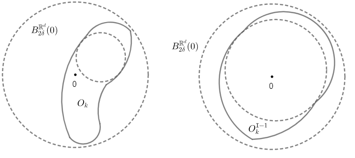
Next, we discuss how the above method to construct a small round ball in $O^{(\texttt{I}-1)}_{k}$ relates to the evolution of the shapes of the sets $\{O_{k},O^{(1)}_{k},\cdots,O^{(\texttt{I}-1)}_{k}\}$ through the iteration process. If $O^{(\texttt{I}-1)}_{k}\subset\mathbb{R}^{d}$ is very close to spherical, then it is easy to verify our algorithm produces a ball contained in $O^{(\texttt{I}-1)}_{k}$. On the other hand, by (26) and (3) in Theorem 1, all the sets $\{O_{k},O^{(1)}_{k},\cdots,O^{(\texttt{I}-1)}_{k}\}$ are contained in $B^{\mathbb{R}^{d}}_{2\delta}(0)$. Since $\sigma^{(i-1)}$ decreases as $i$ increases, comparing to $\{O_{k},O^{(1)}_{k},\cdots,O^{(\texttt{I}-2)}_{k}\}$, $O^{(\texttt{I}-1)}_{k}$ contains a larger ball of radius closer to $2\delta$. In Figure 6, we show an illustration of the sets $O_{k}$ and $O^{(\texttt{I}-1)}_{k}$ for a comparison. Hence, we perform the interpolation after sufficient iterations of Step 1-3 in Algorithm 1.

Figure 6. Both $O_{k}$ and $O^{(\texttt{I}-1)}_{k}$ are contained in $B^{\mathbb{R}^{d}}_{2\delta}(0)$. Left: An illustration of the set $O_{k}\subset\mathbb{R}^{d}$ – $O_{k}$ containing a small round ball. Right: An illustration of the set $O^{(\texttt{I}-1)}_{k}\subset\mathbb{R}^{d}$ – $O^{(\texttt{I}-1)}_{k}$ containing a larger round ball of radius close to $2\delta$.

To make sure that the charts are glued together smoothly and the interpolated points lie on a smooth manifold, we iteratively interpolate the points in the charts $\Phi^{(\texttt{I}-1)}_{i}$ for $i$ from $1$ to $n$. Suppose $\tilde{M}_{k-1}$ is the union of $K(k-1)$ points interpolated in the charts $\{\Phi^{(\texttt{I}-1)}_{i}\}_{i=1}^{k-1}$. We find $B^{\mathbb{R}^{D}}_{\delta}(\textbf{y}^{(\texttt{I}-1)}_{k})\cap\tilde{M}_{k-1}=\{\tilde{\textbf{y}}_{k,1},\cdots,\tilde{\textbf{y}}_{k,L_{k}}\}$. Suppose $\tilde{\textbf{w}}_{k,j}=\mathcal{P}_{\textbf{y}^{(\texttt{I}-1)}_{k}}(\tilde{\textbf{y}}_{k,j})$ and $\tilde{\textbf{z}}_{k,j}=\mathcal{P}^{\bot}_{\textbf{y}^{(\texttt{I}-1)}_{k}}(\tilde{\textbf{y}}_{k,j})$ for $j=1,\cdots,L_{k}$. Since $\Phi^{(\texttt{I}-1)}_{k}$ is a chart of $\iota(M)$ over $B^{\mathbb{R}^{D}}_{2\delta}(\textbf{y}^{(\texttt{I}-1)}_{k})\cap\iota(M)$, we need to predict $F^{(\texttt{I}-1)}_{k}$ in (20) over $\{\tilde{\textbf{u}}_{k,1},\cdots,\tilde{\textbf{u}}_{k,K}\}$. We use $\{\textbf{w}^{(\texttt{I}-1)}_{k,1},\cdots,\textbf{w}^{(\texttt{I}-1)}_{k,N^{(\texttt{I}-1)}_{k}},\tilde{\textbf{w}}_{k,1},\cdots,\tilde{\textbf{w}}_{k,L_{k}}\}$ as the inputs for $F^{(\texttt{I}-1)}_{k}$ and $\{\textbf{z}^{(\texttt{I}-1)}_{k,1},\cdots,\textbf{z}^{(\texttt{I}-1)}_{k,N^{(\texttt{I}-1)}_{k}},\tilde{\textbf{z}}_{k,1},\cdots,\tilde{\textbf{z}}_{k,L_{k}}\}$ as the response variables. The coordinates of the interpolated points around $\hat{\textbf{y}}_{k}$ are provided in (11).

Based on the above discussion, the key idea is contained in Steps 1-3 of Algorithm 1 where we use GP regression to fit the functions $F_{k}$ for $k=1,\cdots,n$. Although there are many ways to fit the unknown functions, we choose GP regression for the following reasons. First, GP regression is flexible. There may be a relatively large deviation from the subspace generated by the eigenvectors corresponding to the $d$ largest eigenvalues of $C_{n,\epsilon}(\textbf{y}_{k})$ to the tangent space of $\iota(M)$ at $\iota(x_{k})$, while the projection from $\iota(M)$ onto the subspace is still a diffeomorphism locally. Hence, the function $F_{k}$ can be quite different from a function dominated by quadratic terms, e.g. the function $G_{x}$ in Proposition 2. We use GP regression to fit $F_{k}$ to avoid unrealistic restrictions. Second, GP regression is a probabilistic approach that automatically provides predictive distributions for the denoised samples. Third, GP regression is an efficient method for interpolation. In particular, we can smoothly merge intersecting charts.

3.6. Evaluation of the performance of the algorithm

In this section, we introduce an approach to evaluate performance of MrGap. The error in prediction is determined by how far the generated points deviate from the embedded submanifold $\iota(M)$. Thus, we introduce the following geometric root mean square error. For any $\textbf{y}\in\mathbb{R}^{D}$, the distance from y to $S\subset\mathbb{R}^{D}$ is defined as

$$\texttt{dist}(\textbf{y},S)=\inf_{\textbf{y}^{\prime}\in S}\|\textbf{y}-\textbf{y}^{\prime}\|_{\mathbb{R}^{D}}.$$

Given $\mathcal{Y}=\{\textbf{y}_{1},\cdots,\textbf{y}_{n}\}\subset\mathbb{R}^{D}$, the geometric root mean square error (GRMSE) from $\mathcal{Y}$ to $S$ is

$$GRMSE(\mathcal{Y},S)=\sqrt{\frac{1}{n}\sum_{i=1}^{n}\texttt{dist}(\textbf{y}_{i},S)^{2}}.$$

Note that $GRMSE(\mathcal{Y},S)=0$ if and only if $\mathcal{Y}$ is in the closure of $S$. Hence, when $S$ is compact, $GRMSE(\mathcal{Y},S)=0$ if and only if $\mathcal{Y}\subset S$.

Remark 2.

The Hausdorff distance is not a good measure of the error from the samples $\{\textbf{y}_{1},\cdots,\textbf{y}_{n}\}$ to $S$. First, it measures maximum distance between two sets rather than average distance. Second, the Hausdorff distance between two sets $A$ and $B$ is $0$ if and only if they have the same closure. Hence, when $\{\textbf{y}_{1},\cdots,\textbf{y}_{n}\}\subset S$, the Hausdorff distance between $\{\textbf{y}_{1},\cdots,\textbf{y}_{n}\}$ and $S$ is still not $0$ unless $S=\{\textbf{y}_{1},\cdots,\textbf{y}_{n}\}$.

In the following proposition, we show that when $S=\iota(M)$ and $\mathcal{Y}_{true}$ is sampled on $\iota(M)$ based on a density function with a positive lower bound, if the sample size of $\mathcal{Y}_{true}$ goes to infinity, then $GRMSE(\mathcal{Y},\mathcal{Y}_{true})$ converges to $GRMSE(\mathcal{Y},\iota(M))$ almost surely. We also provide the convergence rate. The proof of the proposition is in Appendix D.

Proposition 7.

Suppose $\mathcal{Y}=\{\textbf{y}_{1},\cdots,\textbf{y}_{n}\}\subset\mathbb{R}^{D}$. $\{x_{1},\cdots,x_{m}\}$ are samples on $M$ based on a $C^{1}$ p.d.f $\mathrm{q}$ on $M$ such that $\mathrm{q}>\mathrm{q}_{\min}>0$. Let $\mathcal{Y}_{true}=\{\iota(x_{1}),\cdots,\iota(x_{m})\}$. Suppose $C$ is a constant depending on $d$, $D$, $C^{1}$ norm of $\mathrm{q}$, the curvature of $M$ and the second fundamental form of $\iota(M)$, then with probability greater than $1-\frac{1}{m^{2}}$,

$$GRMSE(\mathcal{Y},\mathcal{Y}_{true})^{2}-2rGRMSE(\mathcal{Y},\iota(M))-r^{2}\leq GRMSE(\mathcal{Y},\iota(M))^{2}\leq GRMSE(\mathcal{Y},\mathcal{Y}_{true})^{2},$$

where $r^{d}=\max(\frac{2}{\mathrm{q}_{\min}},(\frac{2C}{\mathrm{q}_{\min}})^{2})\frac{\log m}{m}$.

Note that $\mathrm{q}_{\min}\leq\frac{1}{Vol(M)}$ and the equality holds when $\mathrm{q}$ is uniform. Therefore, the above proposition suggests an efficient way to estimate $GRMSE(\mathcal{Y},\iota(M))$ is sampling $\mathcal{Y}_{true}$ uniformly.

4. Numerical examples

In this section, we demonstrate the performance of MrGap in two examples. The manifold $M$ in the first example is a closed curve, while $M$ in the second example is a torus. In each case, the manifold is isometrically embedded into $\mathbb{R}^{3}$ through $\iota$. We sample points on $\iota(M)$ and add Gaussian noise. We first apply our algorithm to denoise the samples and then interpolate points to approximate $\iota(M)$.

4.1. Cassini Oval in $\mathbb{R}^{3}$

We consider a Cassini Oval $\iota(M)$ in $\mathbb{R}^{3}$ parametrized by $\theta\in[0,2\pi)$,

(28) $$X(\theta)=\sqrt{\cos(2\theta)+\sqrt{\cos(2\theta)^{2}+0.2}}\cos(\theta),$$

$$Y(\theta)=\sqrt{\cos(2\theta)+\sqrt{\cos(2\theta)^{2}+0.2}}\sin(\theta),$$

$$Z(\theta)=0.3\sin(\theta+\pi).$$

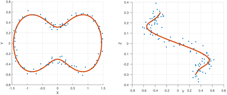
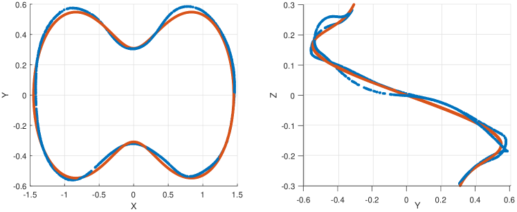
We uniformly sample points $\{\theta_{i}\}_{i=1}^{102}$ on $[0,2\pi)$ to obtain non-uniform samples $\{X(\theta_{i}),Y(\theta_{i}),Z(\theta_{i})\}_{i=1}^{102}$ on $\iota(M)$. Suppose $\eta_{i}\sim\mathcal{N}(0,{\sigma}^{2}I_{3\times 3}),$ with $\sigma=0.04$, $\textbf{y}_{i}=(X(\theta_{i}),Y(\theta_{i}),Z(\theta_{i}))^{\top}+\eta_{i}$ for $i=1,\cdots,102$, and $\mathcal{Y}=\{\textbf{y}_{i}\}_{i=1}^{102}$. We uniformly sample $\{\phi_{i}\}_{i=1}^{10^{5}}$ on $[0,2\pi)$ to obtain $\mathcal{Y}_{true}=\{X(\phi_{i}),Y(\phi_{i}),Z(\phi_{i})\}_{i=1}^{10^{5}}$. We use $\mathcal{Y}_{true}$ to approximate the GRMSE from samples to $\iota(M)$ with $GRMSE(\mathcal{Y},\mathcal{Y}_{true})=0.059$. We plot $\mathcal{Y}$ and $\mathcal{Y}_{true}$ in Figure 7. We apply the MrGap algorithm with $\epsilon=0.3$ and $\delta=0.6$. We iterate Steps 1-3 of Algorithm 1 twice. The estimated covariance parameters in the last round of the iterations are $A^{(1)}=0.048$, $\rho^{(1)}=0.3$ and $\sigma^{(1)}=\sqrt{2\times 10^{-5}}$. The denoised outputs are $\mathcal{X}_{1}=\{\hat{\textbf{y}}_{i}\}_{i=1}^{102}$, with $GRMSE(\mathcal{X}_{1},\mathcal{Y}_{true})=0.0224$. The plot of $\mathcal{X}_{1}$ and $\mathcal{Y}_{true}$ is in Figure 15 in Appendix G. When we apply Algorithm 2 , we choose $K=20$, i.e. we construct $102$ charts and we interpolate $20$ points in each chart. The outputs are $\mathcal{X}_{2}=\{\tilde{\textbf{y}}_{i}\}_{i=1}^{2040}$ with $GRMSE(\mathcal{X}_{2},\mathcal{Y}_{true})=0.0216$. We plot $\mathcal{X}_{2}$ and $\mathcal{Y}_{true}$ in Figure 8. We provide a comparison of MrGap and the principal graph algorithm for this example in Appendix G.

Figure 7. $\mathcal{Y}$ contains $102$ noisy points around the Cassani Oval $\iota(M)$ and $\mathcal{Y}_{true}$ contains $10^{5}$ points on $\iota(M)$. The left and the right panels show the XY plot and YZ plot of $\mathcal{Y}$ and $\mathcal{Y}_{true}$ respectively. The blue points are $\mathcal{Y}$ and the red points are $\mathcal{Y}_{true}$. We use $\mathcal{Y}_{true}$ to estimate the GRMSE from samples to $\iota(M)$ with $GRMSE(\mathcal{Y},\mathcal{Y}_{true})=0.059$.

Figure 8. $\mathcal{X}_{2}$ contains $2040$ interpolated points by the MrGap algorithm. The left and the right panels show the XY plot and YZ plot of $\mathcal{X}_{2}$ and $\mathcal{Y}_{true}$ respectively. The blue points are $\mathcal{X}_{2}$ and the red points are $\mathcal{Y}_{true}$. We use $\mathcal{Y}_{true}$ to estimate the GRMSE from samples to $\iota(M)$ with $GRMSE(\mathcal{X}_{2},\mathcal{Y}_{true})=0.0216$.

4.2. Torus in $\mathbb{R}^{3}$

We consider a torus $\iota(M)$ in $\mathbb{R}^{3}$ parametrized by $u,v\in[0,2\pi)$,

$$X(u,v)=(2+0.8\cos(u))\cos(v),\quad Y(u,v)=(2+0.8\cos(u))\sin(v),\quad Z(u,v)=0.8\sin(u).$$

We randomly sample $558$ points $\{\iota(x_{i})\}_{i=1}^{558}$ based on the uniform density function on $\iota(M)$. Let $\eta_{i}\sim\mathcal{N}(0,{\sigma}^{2}I_{3\times 3}),$ with $\sigma=0.12$, $\textbf{y}_{i}=\iota(x_{i})+\eta_{i}$ for $i=1,\cdots,558$, and $\mathcal{Y}=\{\textbf{y}_{i}\}_{i=1}^{558}$. We randomly sample $3.2\times 10^{5}$ points based on the uniform density function on $\iota(M)$ to form $\mathcal{Y}_{true}$. 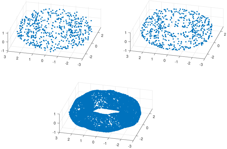We calculate the GRMSE from $\mathcal{Y}$ to $\mathcal{Y}_{true}$ which is $GRMSE(\mathcal{Y},\mathcal{Y}_{true})=0.1238$. We plot $\mathcal{Y}$ in Figure 9. We apply the MrGap algorithm with $\epsilon=0.8$ and $\delta=1$. We iterate Steps 1-3 of Algorithm 1 twice. The estimated covariance parameters in the last round of the iterations are $A^{(1)}=0.2$, $\rho^{(1)}=1.1$ and $\sigma^{(1)}=\sqrt{0.007}$. The final denoised outputs are $\mathcal{X}_{1}=\{\hat{\textbf{y}}_{i}\}_{i=1}^{558}$ with $GRMSE(\mathcal{X}_{1},\mathcal{Y}_{true})=0.0544$. We plot $\mathcal{X}_{1}$ in Figure 9. As in the previous example, we choose $K=20$ in applying algorithm 2. The outputs are $\mathcal{X}_{2}=\{\tilde{\textbf{y}}_{i}\}_{i=1}^{11160}$ with $GRMSE(\mathcal{X}_{2},\mathcal{Y}_{true})=0.0605$. We plot $\mathcal{X}_{2}$ in Figure 9.

Figure 9. $\mathcal{Y}$ contains $558$ noisy points around the torus $\iota(M)$ and $\mathcal{Y}_{true}$ contains $3.2\times 10^{5}$ points on the torus $\iota(M)$. $\mathcal{X}_{1}$ contains $558$ denoised points on $\iota(M)$ by the MrGap algorithm. $\mathcal{X}_{2}$ contains $11160$ interpolated points on $\iota(M)$ by the MrGap algorithm. We use $\mathcal{Y}_{true}$ to estimate the GRMSE from samples to $\iota(M)$. Top left: Original data $\mathcal{Y}$ with $GRMSE(\mathcal{Y},\mathcal{Y}_{true})=0.1238$. Top right: Fits from Mr Gap $\mathcal{X}_{1}$ with $GRMSE(\mathcal{X}_{1},\mathcal{Y}_{true})=0.0544$. Bottom: Interpolated fits from Mr Gap $\mathcal{X}_{2}$ with $GRMSE(\mathcal{X}_{2},\mathcal{Y}_{true})=0.0605$.

5. Near-infrared reflectance spectra of wheat samples

Recall the NIRS data from [18] introduced in Section 1 and Figure 1.We apply the MrGap algorithm with $\epsilon=0.7$ and $\delta=0.9$ through the iteration process. We repeat Steps 1-3 of Algorithm 1 three times. The estimated covariance parameters in the last round of the iterations are $A^{(2)}=3\times 10^{-6}$, $\rho^{(2)}=0.6$ and $\sigma^{(2)}=\sqrt{1\times 10^{-6}}$. The denoised outputs are $\mathcal{X}_{1}=\{\hat{\textbf{y}}_{i}=\textbf{y}^{(3)}_{i}\}_{i=1}^{86}$. When we apply Algorithm 2 , we choose $K=30$ so that we interpolate $2580$ points in total on the curve. The outputs are $\mathcal{X}_{2}=\{\tilde{\textbf{y}}_{i}\}_{i=1}^{2580}$.

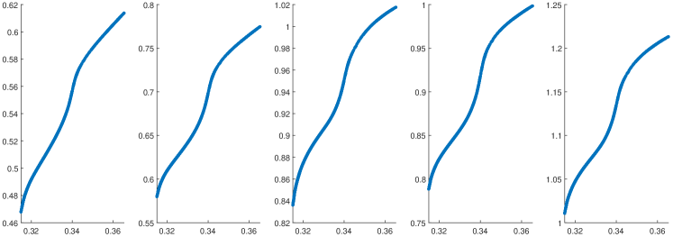
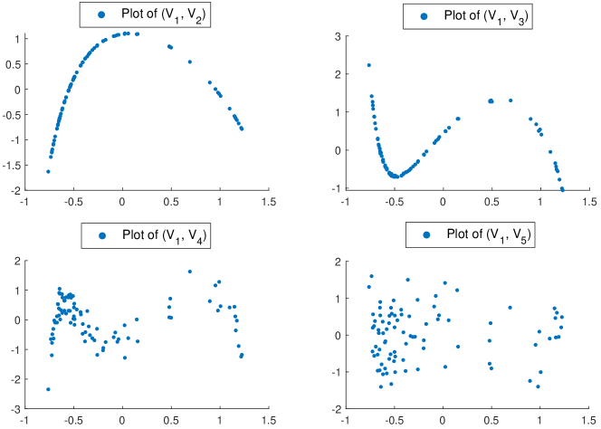
To visualize the results, in Figure 2, we plot the denoised reflectance spectra $\mathcal{X}_{1}$ corresponding to the $86$ samples and the denoised spectrum corresponding to the $28$th sample. In Figure 10, we plot the projections of $\mathcal{X}_{1}$ and $\mathcal{X}_{2}$ onto the $(1,140),(1,280),(1,420),(1,560),(1,700)$ coordinate planes. In other words, we plot the pairs $(\hat{\textbf{y}}_{i}(1),\hat{\textbf{y}}_{i}(140j))_{i=1}^{86}$ and $(\tilde{\textbf{y}}_{i}(1),\tilde{\textbf{y}}_{i}(140j))_{i=1}^{2580}$ for $j=1,\cdots,5$.

Figure 10. Suppose $\{\hat{\textbf{y}}_{i}\}_{i=1}^{86}$ are the denoised outputs and $\{\tilde{\textbf{y}}_{i}\}_{i=1}^{2580}$ are interpolated points. Top row from left to right: $(\hat{\textbf{y}}_{i}(1),\hat{\textbf{y}}_{i}(140j))_{i=1}^{86}$ for $j=1,\cdots,5$. Bottom row from left to right: $(\tilde{\textbf{y}}_{i}(1),\tilde{\textbf{y}}_{i}(140j))_{i=1}^{2580}$ for $j=1,\cdots,5$.

6. Discussion

We have proposed a manifold recontruction algorithm, MrGap, which relies on Gaussian processes to obtain a smoothly interpolated estimate of an unknown manifold by combining local charts. Key tuning parameters, including the measurement error noise and GP covariance parameters, are estimated by maximizing the marginal likelihood obtained in marginalizing out the unknown functions over their GP priors. This is a common approach for tuning parameter choice in GP-based models. In the reflectance spectra examples, we first apply diffusion map to obtain insight into the appropriate $d$, and then use this $d$ in our implementations of MrGap.

There are many interesting areas for future research. One direction is to further refine the MrGap algorithm, with a focus on computational scalability to large sample sizes and obtaining an accurate characterization of uncertainty in manifold learning. Another direction is to consider more elaborate data structures, such as when only a subset of the observed data have a manifold structure. In addition, it will be interesting to build on the theory we developed in this paper to obtain rates of convergence and other asymptotic properties.

Appendix A Proof of Proposition 3

A.1. Preliminary lemmas

We introduce some notation. Suppose $S$ is a subset of $M$. Then $\chi_{S}(x)$ is the characteristic function on $S$. For $S_{1},S_{2}\subset M$, let $S_{1}\Delta S_{2}=(S_{1}\setminus S_{2})\cup(S_{2}\setminus S_{1})$ be the symmetric difference. Let $d_{M}(x,x^{\prime})$ be the geodesic distance between $x$ and $x^{\prime}$ in $M$. Let $B_{r}(x)\subset M$ be the open geodesic ball of radius $r$ centered at $x\in M$.

First, we have the following lemma about the geodesic distance between $x$ and $x^{\prime}$ on $M$ and the Euclidean distance between $\iota(x)$ and $\iota(x^{\prime})$ in $\mathbb{R}^{D}$. The proof of the lemma is available in [33].

Lemma 1.

Fix $x\in M$. For $\textbf{u}\in T_{x}M\approx\mathbb{R}^{d}$ with $\|\textbf{u}\|_{\mathbb{R}^{d}}$ sufficiently small, if $x^{\prime}=exp_{x}(\textbf{u})$, then

$$\iota(x^{\prime})-\iota(x)= \,\iota_{*}\textbf{u}+\frac{1}{2}\textup{I}\!\textup{I}_{x}(\textbf{u},\textbf{u})+O(\|\textbf{u}\|^{3}_{\mathbb{R}^{d}}),$$

where $\textup{I}\!\textup{I}_{x}$ is the second fundamental form of $\iota(M)$ at $x$. Moreover,

$$\|\iota(x^{\prime})-\iota(x)\|_{\mathbb{R}^{D}}=\|\textbf{u}\|_{\mathbb{R}^{d}}-\frac{1}{24}\Big{\|}\textup{I}\!\textup{I}_{x}\Big{(}\frac{\textbf{u}}{\|\textbf{u}\|_{\mathbb{R}^{d}}},\frac{\textbf{u}}{\|\textbf{u}\|_{\mathbb{R}^{d}}}\Big{)}\Big{\|}^{2}_{\mathbb{R}^{D}}\|\textbf{u}\|^{3}_{\mathbb{R}^{d}}+O(\|\textbf{u}\|^{4}_{\mathbb{R}^{d}}).$$

In other words,

$$\|\textbf{u}\|_{\mathbb{R}^{d}}=\|\iota(x^{\prime})-\iota(x)\|_{\mathbb{R}^{D}}+\frac{1}{24}\Big{\|}\textup{I}\!\textup{I}_{x}\Big{(}\frac{\textbf{u}}{\|\textbf{u}\|_{\mathbb{R}^{d}}},\frac{\textbf{u}}{\|\textbf{u}\|_{\mathbb{R}^{d}}}\Big{)}\Big{\|}^{2}_{\mathbb{R}^{D}}\|\iota(x^{\prime})-\iota(x)\|^{3}_{\mathbb{R}^{D}}+O(\|\iota(x^{\prime})-\iota(x)\|^{4}_{\mathbb{R}^{D}}).$$

Next, we introduce the following lemma about the volume form on $M$. The proof of the lemma is available in [9].

Lemma 2.

Fix $x\in M$. For $\textbf{u}\in T_{x}M\approx\mathbb{R}^{d}$ with $\|\textbf{u}\|_{\mathbb{R}^{d}}$ sufficiently small, the volume form has the following expansion

$$dV=\Big{(}1-\sum_{i,j=1}^{d}\frac{1}{6}\texttt{Ric}_{x}(e^{\prime}_{i},e^{\prime}_{j})u_{i}u_{j}+O(\|\textbf{u}\|^{3}_{\mathbb{R}^{d}})\Big{)}d\textbf{u},$$

where $\textbf{u}=\sum_{i=1}^{d}u_{i}e^{\prime}_{i}$ and $\texttt{Ric}_{x}$ is the Ricci curvature tensor of $M$ at $x$. Consequently,

$$\texttt{Vol}(B_{r}(x))=\texttt{Vol}(B^{\mathbb{R}^{d}}_{1})r^{d}\Big{(}1-\frac{\texttt{S}_{x}}{6(d+2)}r^{2}+O(r^{4})\Big{)},$$

where $\texttt{S}_{x}$ is the scalar curvature of $M$ at $x$.

Recall that $G_{\sigma}(\eta)$ is the $\mathcal{N}(0,\sigma^{2}I_{D\times D})$ probability density function of $\eta$:

$$G_{\sigma}(\eta)=\frac{1}{(2\pi\sigma^{2})^{\frac{D}{2}}}e^{-\frac{\|\eta\|^{2}_{\mathbb{R}^{D}}}{2\sigma^{2}}}.$$

We have the following Lemma describing bounds on $G_{\sigma}(\eta)$.

Lemma 3.

1. If $\frac{t}{\sigma}\geq\sqrt{2}(D-2)$, then $\int_{\|\eta\|_{\mathbb{R}^{D}}\geq t}G_{\sigma}(\eta)d\eta\leq\frac{2}{\Gamma(\frac{D}{2})}e^{-\frac{t^{2}}{4\sigma^{2}}}.$

2. $\int_{\mathbb{R}^{D}}\eta(i)^{2}G_{\sigma}(\eta)d\eta\leq\sigma^{2},$ for $i=1,\cdots,D$.

Proof.

(1) By the change of variables in the spherical coordinates,

$$\int_{\|\eta\|_{\mathbb{R}^{D}}\geq t}G_{\sigma}(\eta)d\eta=\frac{1}{(2\pi\sigma^{2})^{\frac{D}{2}}}(2\sigma^{2})^{\frac{D}{2}}|S^{D-1}|\int_{\frac{t}{\sqrt{2}\sigma}}^{\infty}r^{D-1}e^{-r^{2}}dr=\frac{|S^{D-1}|}{\pi^{\frac{D}{2}}}\int_{\frac{t}{\sqrt{2}\sigma}}^{\infty}r^{D-1}e^{-r^{2}}dr.$$

Since $\frac{r}{2}\geq\log(r)$ for all $r>0$, when $r\geq D-2$, we have $D-2\leq\frac{r^{2}}{2\log(r)}$. Hence, $r^{D-2}e^{-r^{2}}\leq e^{-\frac{r^{2}}{2}}$. If $\frac{t}{\sigma}\geq\sqrt{2}(D-2)$, then

$$\int_{\|\eta\|_{\mathbb{R}^{D}}\geq t}G_{\sigma}(\eta)d\eta\leq\frac{|S^{D-1}|}{\pi^{\frac{D}{2}}}\int_{\frac{t}{\sqrt{2}\sigma}}^{\infty}e^{-\frac{r^{2}}{2}}rdr=\frac{2}{\Gamma(\frac{D}{2})}e^{-\frac{t^{2}}{4\sigma^{2}}}.$$

(2) follows from the change of variables in the spherical coordinates and the symmetry of $\mathbb{R}^{D}$. ∎

Recall that we have $\iota(x_{k})=0\in\mathbb{R}^{D}$. For $1<\beta\leq\alpha-\frac{1}{2}$, we define the following terms which we will use in our discussion.

$$F_{1}(\iota(x),\eta,\eta_{k})=(\iota(x)+\eta-\eta_{k})(\iota(x)+\eta-\eta_{k})^{\top}\chi(\frac{\|\iota(x)+\eta-\eta_{k}\|_{\mathbb{R}^{D}}}{\epsilon}),$$

$$E_{1}=\int_{\|\eta\|_{\mathbb{R}^{D}}<\epsilon^{\beta}}\int_{M}F_{1}(\iota(x),\eta,\eta_{k})P(x)G_{\sigma}(\eta)dVd\eta,$$

$$E_{2}=\int_{\|\eta\|_{\mathbb{R}^{D}}\geq\epsilon^{\beta}}\int_{M}F_{1}(\iota(x),\eta,\eta_{k})P(x)G_{\sigma}(\eta)dVd\eta,$$

$$E_{3}=\int_{\|\eta\|_{\mathbb{R}^{D}}<\epsilon^{\beta}}\int_{M}(\iota(x)+\eta-\eta_{k})(\iota(x)+\eta-\eta_{k})^{\top}\chi_{B_{\epsilon}(x_{k})}(x)P(x)G_{\sigma}(\eta)dVd\eta.$$

Lemma 4.

Suppose $\epsilon$ is small enough depending on $d$ and $D$. Suppose $\sigma=\epsilon^{\alpha}$ and $1<\beta\leq\alpha-\frac{1}{2}$. Then $|e_{i}^{\top}E_{2}e_{j}|\leq\epsilon^{d+5}$ for all $1\leq i,j\leq D$.

Proof.

When $\|\iota(x)+\eta-\eta_{k}\|_{\mathbb{R}^{D}}\leq\epsilon$, $\chi(\frac{\|\iota(x)+\eta-\eta_{k}\|_{\mathbb{R}^{D}}}{\epsilon})\leq 1$. When $\|\iota(x)+\eta-\eta_{k}\|_{\mathbb{R}^{D}}>\epsilon$, $\chi(\frac{\|\iota(x)+\eta-\eta_{k}\|_{\mathbb{R}^{D}}}{\epsilon})=0$. Hence, for all $1\leq i,j\leq D$ and all $x$, we have

$$|e_{i}^{\top}(\iota(x)+\eta-\eta_{k})(\iota(x)+\eta-\eta_{k})^{\top}e_{j}|\chi(\frac{\|\iota(x)+\eta-\eta_{k}\|_{\mathbb{R}^{D}}}{\epsilon})\leq\epsilon^{2}.$$

Next, we bound $|e_{i}^{\top}E_{2}e_{j}|$,

$$|e_{i}^{\top}E_{2}e_{j}|\leq \int_{\|\eta\|_{\mathbb{R}^{D}}\geq\epsilon^{\beta}}\int_{M}|e_{i}^{\top}(\iota(x)+\eta-\eta_{k})(\iota(x)+\eta-\eta_{k})^{\top}e_{j}|$$

$$\hskip 113.81102pt\times\chi(\frac{\|\iota(x)+\eta-\eta_{k}\|_{\mathbb{R}^{D}}}{\epsilon})P(x)G_{\sigma}(\eta)dVd\eta$$

$$\leq \int_{\|\eta\|_{\mathbb{R}^{D}}\geq\epsilon^{\beta}}\int_{M}\epsilon^{2}P(x)G_{\sigma}(\eta)dVd\eta=\int_{\|\eta\|_{\mathbb{R}^{D}}\geq\epsilon^{\beta}}\epsilon^{2}G_{\sigma}(\eta)d\eta\int_{M}P(x)dV$$

$$\leq \int_{\|\eta\|_{\mathbb{R}^{D}}\geq\epsilon^{\beta}}\epsilon^{2}G_{\sigma}(\eta)d\eta.$$

We apply Fubini’s theorem in the second to last step and the fact that $P(x)$ is a probability density function on $M$ in the last step. Since $\beta\leq\alpha-\frac{1}{2}$, if $\epsilon^{2(\beta-\alpha)}\geq\frac{1}{\epsilon}\geq 2\sqrt{2}(D-2)$, then by Lemma 3,

$$|e_{i}^{\top}E_{2}e_{j}|\leq\frac{2\epsilon^{2}}{\Gamma(\frac{D}{2})}e^{-\frac{1}{4\epsilon^{2(\alpha-\beta)}}}\leq\frac{2\epsilon^{2}}{\Gamma(\frac{D}{2})}e^{-\frac{1}{4\epsilon}}.$$

We apply $\beta\leq\alpha-\frac{1}{2}$ in the last step again. Since $\Gamma(\frac{D}{2})>1$, when $\epsilon$ is small enough depending on $d$ and $D$, we have $|e_{i}^{\top}E_{2}e_{j}|\leq\epsilon^{d+5}$. ∎

Lemma 5.

Suppose $\epsilon$ is small enough depending on the second fundamental form of $\iota(M)$. Let $W_{ij}(x)=|e_{i}^{\top}(\iota(x)+\eta-\eta_{k})(\iota(x)+\eta-\eta_{k})^{\top}e_{j}|$. Suppose $1<\beta\leq 3$. If $\|\eta\|_{\mathbb{R}^{D}}\leq\epsilon^{\beta}$ $\|\eta_{k}\|_{\mathbb{R}^{D}}\leq\epsilon^{\beta}$, then for $x\in B_{\epsilon+3\epsilon^{\beta}}(x_{k})$

$$W_{ij}(x)\leq 49\epsilon^{2},\quad\mbox{for $1\leq i,j\leq d$,}$$

$$W_{ij}(x)\leq C_{3}(\epsilon^{3}+\epsilon^{1+\beta}),\quad\mbox{for $1\leq i\leq d$ and $d+1\leq j\leq D$,}$$

$$W_{ij}(x)\leq C_{3}(\epsilon^{3}+\epsilon^{1+\beta}),\quad\mbox{for $d+1\leq i\leq D$ and $1\leq j\leq d$,}$$

$$W_{ij}(x)\leq C_{3}(\epsilon^{4}+\epsilon^{2\beta}),\quad\mbox{for $d+1\leq i,j\leq D$},$$

where $C_{3}$ is a constant depending on the second fundamental form of $\iota(M)$.

Suppose $\beta>3$. If $\|\eta\|_{\mathbb{R}^{D}}\leq\epsilon^{\beta}$ $\|\eta_{k}\|_{\mathbb{R}^{D}}\leq\epsilon^{\beta}$, then for $x\in B_{\epsilon+3\epsilon^{3}}(x_{k})$

$$W_{ij}(x)\leq 49\epsilon^{2},\quad\mbox{for $1\leq i,j\leq d$,}$$

$$W_{ij}(x)\leq 2C_{3}\epsilon^{3},\quad\mbox{for $1\leq i\leq d$ and $d+1\leq j\leq D$,}$$

$$W_{ij}(x)\leq 2C_{3}\epsilon^{3},\quad\mbox{for $d+1\leq i\leq D$ and $1\leq j\leq d$,}$$

$$W_{ij}(x)\leq 2C_{3}\epsilon^{4},\quad\mbox{for $d+1\leq i,j\leq D$.}$$

Proof.

Since $\|\eta\|_{\mathbb{R}^{D}}<\epsilon^{\beta}$ and $\|\eta_{k}\|_{\mathbb{R}^{D}}\leq\epsilon^{\beta}$, we have

(29) $$|e_{i}^{\top}(\iota(x)+\eta-\eta_{k})(\iota(x)+\eta-\eta_{k})^{\top}e_{j}|$$

$$\leq (|e_{i}^{\top}\iota(x)|+|e_{i}^{\top}\eta|+|e_{i}^{\top}\eta_{k}|)(|\iota(x)^{\top}e_{j}|+|\eta^{\top}e_{j}|+|\eta_{k}^{\top}e_{j}|)$$

$$\leq (|e_{i}^{\top}\iota(x)|+2\epsilon^{\beta})(|\iota(x)^{\top}e_{j}|+2\epsilon^{\beta}).$$

For any $x\in B_{\epsilon+3\epsilon^{\beta}}(x_{k})$, suppose $x=\exp_{x_{k}}(\textbf{u})$ for $\textbf{u}\in T_{x_{k}}M\approx\mathbb{R}^{d}$. Then, $\|\textbf{u}\|_{\mathbb{R}^{d}}\leq\epsilon+3\epsilon^{\beta}$. By Lemma 1, we have

$$\iota(x)=\iota_{*}\textbf{u}+\frac{1}{2}\textup{I}\!\textup{I}_{x}(\textbf{u},\textbf{u})+O(\|\textbf{u}\|^{3}_{\mathbb{R}^{d}})$$

Since $\{e_{1},\cdots,e_{d}\}$ form a basis of $\iota_{*}T_{x_{k}}M$, they are perpendicular to $\textup{I}\!\textup{I}_{x}(\textbf{u},\textbf{u})$. Since $1<\beta$, when $\epsilon$ is small enough depending on the second fundamental form of $\iota(M)$, we have $|e_{i}^{\top}\iota(x)|\leq 5\epsilon$ for $i=1,\cdots,d$. Similarly, since $\{e_{d+1},\cdots,e_{D}\}$ form a basis of $\iota_{*}T_{x_{k}}M^{\bot}$, they are perpendicular to $\iota_{*}\textbf{u}$. When $\epsilon$ is small enough depending on the second fundamental form of $\iota(M)$, we have $|e_{i}^{\top}\iota(x)|\leq C_{2}\epsilon^{2}$ for $i=d+1,\cdots,D$, where $C_{2}$ is a constant depending on the second fundamental form of $\iota(M)$. If we substitute the bounds of $|e_{i}^{\top}\iota(x)|$ into (29), then after the simplification, for any $\|\eta\|_{\mathbb{R}^{D}}<\epsilon^{\beta}$, $\|\eta_{k}\|_{\mathbb{R}^{D}}\leq\epsilon^{\beta}$ and $x\in B_{\epsilon+3\epsilon^{\beta}}(x_{k})$, we have

$$|e_{i}^{\top}(\iota(x)+\eta-\eta_{k})(\iota(x)+\eta-\eta_{k})^{\top}e_{j}|\leq 49\epsilon^{2},\quad\mbox{for $1\leq i,j\leq d$,}$$

$$|e_{i}^{\top}(\iota(x)+\eta-\eta_{k})(\iota(x)+\eta-\eta_{k})^{\top}e_{j}|\leq C_{3}(\epsilon^{3}+\epsilon^{1+\beta}),\quad\mbox{for $1\leq i\leq d$ and $d+1\leq j\leq D$}$$

$$|e_{i}^{\top}(\iota(x)+\eta-\eta_{k})(\iota(x)+\eta-\eta_{k})^{\top}e_{j}|\leq C_{3}(\epsilon^{3}+\epsilon^{1+\beta}),\quad\mbox{for $d+1\leq i\leq D$ and $1\leq j\leq d$}$$

$$|e_{i}^{\top}(\iota(x)+\eta-\eta_{k})(\iota(x)+\eta-\eta_{k})^{\top}e_{j}|\leq C_{3}(\epsilon^{4}+\epsilon^{2\beta}),\quad\mbox{for $d+1\leq i,j\leq D$},$$

where $C_{3}$ is a constant depending on the second fundamental form of $\iota(M)$. The proof for the case when $\beta>3$ is similar. ∎

Lemma 6.

Suppose $\epsilon$ is small enough depending on the scalar curvature of $M$ and the second fundamental form of $\iota(M)$. Suppose $1<\beta$. If $\|\eta_{k}\|_{\mathbb{R}^{D}}\leq\epsilon^{\beta}$ then

$$E_{1}=E_{3}+\begin{bmatrix}O(\epsilon^{d+1+\beta}+\epsilon^{d+4})&O(\epsilon^{d+2+\beta}+\epsilon^{d+2\beta}+\epsilon^{d+5})\\ O(\epsilon^{d+2+\beta}+\epsilon^{d+2\beta}+\epsilon^{d+5})&O(\epsilon^{d+3+\beta}+\epsilon^{d-1+3\beta}+\epsilon^{d+6})\\ \end{bmatrix},$$

where the top left block is a $d$ by $d$ matrix and the constant factors in the four blocks depend on $d$, $P_{M}$ and the second fundamental form of $\iota(M)$.

Proof.

Let $A(\eta)=\{x\in M\hskip 2.84526pt|\hskip 2.84526pt\|\iota(x)+\eta-\eta_{k}\|_{\mathbb{R}^{D}}\leq\epsilon\mbox{ for a fixed }\|\eta\|_{\mathbb{R}^{D}}<\epsilon^{\beta}\}$. Since $\|\eta\|_{\mathbb{R}^{D}}<\epsilon^{\beta}$ and $\|\eta_{k}\|_{\mathbb{R}^{D}}\leq\epsilon^{\beta}$, by the triangle inequality, if $x\in A(\eta)$, then $\epsilon-2\epsilon^{\beta}\leq\|\iota(x)\|_{\mathbb{R}^{D}}\leq\epsilon+2\epsilon^{\beta}$. If $1<\beta\leq 3$, when $\epsilon$ is small enough depending on the second fundamental form of $\iota(M)$, by Lemma 1, we have $\epsilon-2\epsilon^{\beta}\leq d(x,x_{k})<\epsilon+3\epsilon^{\beta}$. Hence, $B_{\epsilon-2\epsilon^{\beta}}(x_{k})\subset A(\eta)\subset B_{\epsilon+3\epsilon^{\beta}}(x_{k})$ which implies $A(\eta)\Delta B_{\epsilon}\subset B_{\epsilon+3\epsilon^{\beta}}(x_{k})\setminus B_{\epsilon-2\epsilon^{\beta}}(x_{k})$. Since $1<\beta\leq 3$, when $\epsilon$ is small enough depending on the scalar curvature of $M$, by Lemma 2, for all $\|\eta\|_{\mathbb{R}^{D}}<\epsilon^{\beta}$ we have

$$\texttt{Vol}(A(\eta)\Delta B_{\epsilon}(x_{k}))\leq\texttt{Vol}(B_{\epsilon+3\epsilon^{\beta}}(x_{k}))-\texttt{Vol}(B_{\epsilon-2\epsilon^{\beta}}(x_{k}))\leq 6\texttt{Vol}(B^{\mathbb{R}^{d}}_{1})d\epsilon^{d-1+\beta}=C_{1}(d)\epsilon^{d-1+\beta},$$

where $C_{1}(d)=6d\texttt{Vol}(B^{\mathbb{R}^{d}}_{1})$ is a constant only depending on $d$. Similarly, if $\beta>3$, then for all $\|\eta\|_{\mathbb{R}^{D}}<\epsilon^{\beta}$ we have $A(\eta)\Delta B_{\epsilon}\subset B_{\epsilon+3\epsilon^{3}}(x_{k})\setminus B_{\epsilon-2\epsilon^{3}}(x_{k})$ and

$$\texttt{Vol}(A(\eta)\Delta B_{\epsilon}(x_{k}))\leq C_{1}(d)\epsilon^{d+2}.$$

Observe that for a fixed $\|\eta\|_{\mathbb{R}^{D}}<\epsilon^{\beta}$, $|\chi_{A(\eta)}(x)-\chi_{B_{\epsilon}(x_{k})}(x)|\leq\chi_{A(\eta)\Delta B_{\epsilon}(x_{k})}(x)$. Moreover, we have $\chi_{A(\eta)}(x)=\chi(\frac{\|\iota(x)+\eta-\eta_{k}\|_{\mathbb{R}^{D}}}{\epsilon})$. Hence,

(30) $$|e_{i}^{\top}(E_{1}-E_{3})e_{j}|$$

$$\leq \int_{\|\eta\|_{\mathbb{R}^{D}}<\epsilon^{\beta}}\int_{M}|e_{i}^{\top}(\iota(x)+\eta-\eta_{k})(\iota(x)+\eta-\eta_{k})^{\top}e_{j}||\chi_{A(\eta)}(x)-\chi_{B_{\epsilon}(x_{k})}(x)|P(x)G_{\sigma}(\eta)dVd\eta$$

$$\leq \int_{\|\eta\|_{\mathbb{R}^{D}}<\epsilon^{\beta}}\int_{M}|e_{i}^{\top}(\iota(x)+\eta-\eta_{k})(\iota(x)+\eta-\eta_{k})^{\top}e_{j}|\chi_{A(\eta)\Delta B_{\epsilon}(x_{k})}(x)P(x)G_{\sigma}(\eta)dVd\eta$$

$$\leq \Big{(}\sup_{\|\eta\|_{\mathbb{R}^{D}}<\epsilon^{\beta},x\in A(\eta)\Delta B_{\epsilon}(x_{k})}|e_{i}^{\top}(\iota(x)+\eta-\eta_{k})(\iota(x)+\eta-\eta_{k})^{\top}e_{j}|\Big{)}$$

$$\hskip 113.81102pt\times\int_{\|\eta\|_{\mathbb{R}^{D}}<\epsilon^{\beta}}\int_{M}\chi_{A(\eta)\Delta B_{\epsilon}(x_{k})}(x)P(x)G_{\sigma}(\eta)dVd\eta$$

$$\leq \Big{(}\sup_{\|\eta\|_{\mathbb{R}^{D}}<\epsilon^{\beta},x\in A(\eta)\Delta B_{\epsilon}(x_{k})}|e_{i}^{\top}(\iota(x)+\eta-\eta_{k})(\iota(x)+\eta-\eta_{k})^{\top}e_{j}|\Big{)}P_{M}\Big{(}\sup_{\|\eta\|_{\mathbb{R}^{D}}<\epsilon^{\beta}}\texttt{Vol}(A(\eta)\Delta B_{\epsilon}(x_{k}))\Big{)}$$

Recall that if $1<\beta\leq 3$, for any $\|\eta\|_{\mathbb{R}^{D}}<\epsilon^{\beta}$, $A(\eta)\Delta B_{\epsilon}(x_{k})\subset B_{\epsilon+3\epsilon^{\beta}}(x_{k})\setminus B_{\epsilon-2\epsilon^{\beta}}(x_{k})\subset B_{\epsilon+3\epsilon^{\beta}}(x_{k})$. Hence, if we substitute the bounds in Lemma 5 into (30), then we conclude that when $1<\beta\leq 3$ and $\epsilon$ is small enough depending on the scalar curvature of $M$ and the second fundamental form of $\iota(M)$,

$$E_{1}=E_{3}+\begin{bmatrix}O(\epsilon^{d+1+\beta})&O(\epsilon^{d+2+\beta}+\epsilon^{d+2\beta})\\ O(\epsilon^{d+2+\beta}+\epsilon^{d+2\beta})&O(\epsilon^{d+3+\beta}+\epsilon^{d-1+3\beta})\\ \end{bmatrix},$$

where the top left block is a $d$ by $d$ matrix and the constant factors depend on $d$, $P_{M}$ and the second fundamental form of $\iota(M)$.

When $\beta>3$ and $\epsilon$ is small enough depending on the scalar curvature of $M$ and the second fundamental form of $\iota(M)$, we have $A(\eta)\Delta B_{\epsilon}\subset B_{\epsilon+3\epsilon^{3}}(x_{k})\setminus B_{\epsilon-2\epsilon^{3}}(x_{k})$. Hence, if we substitute the bounds in Lemma 5 into (30), then

$$E_{1}=E_{3}+\begin{bmatrix}O(\epsilon^{d+4})&O(\epsilon^{d+5})\\ O(\epsilon^{d+5})&O(\epsilon^{d+6})\\ \end{bmatrix},$$

where the top left block is a $d$ by $d$ matrix and the constant factors depend on $d$, $P_{M}$ and the second fundamental form of $\iota(M)$. The statement of the lemma follows from combining the cases when $1<\beta\leq 3$ and $\beta>3$. ∎

Lemma 7.

Suppose $\epsilon$ is small enough depending on the scalar curvature of $M$ and $D$. Suppose $1<\beta\leq\alpha-\frac{1}{2}$. If $\sigma=\epsilon^{\alpha}$ and $\|\eta_{k}\|_{\mathbb{R}^{D}}\leq\epsilon^{\beta}$, then

$$E_{3}= \frac{|S^{d-1}|{P}(x_{k})}{d(d+2)}\epsilon^{d+2}\begin{bmatrix}I_{d\times d}&0\\ 0&0\\ \end{bmatrix}+O(\epsilon^{d+4}+\epsilon^{d+2\beta}),$$

where $O(\epsilon^{d+4}+\epsilon^{d+2\beta})$ represents a $D$ by $D$ matrix whose entries are of order $O(\epsilon^{d+4}+\epsilon^{d+2\beta})$. The constants in $O(\epsilon^{d+4}+\epsilon^{d+2\beta})$ depend on $d$, $C^{2}$ norm of $P$, the second fundamental form of $\iota(M)$ and its derivative and the Ricci curvature of $M$.

Proof.

(31) $$E_{3}= \int_{\|\eta\|_{\mathbb{R}^{D}}<\epsilon^{\beta}}\int_{M}(\iota(x)+\eta-\eta_{k})(\iota(x)+\eta-\eta_{k})^{\top}\chi_{B_{\epsilon}(x_{k})}(x)P(x)G_{\sigma}(\eta)dVd\eta$$

$$= \int_{\|\eta\|_{\mathbb{R}^{D}}<\epsilon^{\beta}}\int_{M}\Big{(}\iota(x)\iota(x)^{\top}+\eta\iota(x)^{\top}-\eta_{k}\iota(x)^{\top}+\iota(x)\eta^{\top}+\eta\eta^{\top}$$

$$-\eta_{k}\eta^{\top}-\iota(x)\eta_{k}^{\top}-\eta\eta_{k}^{\top}+\eta_{k}\eta_{k}^{\top}\Big{)}\chi_{B_{\epsilon}(x_{k})}(x)P(x)G_{\sigma}(\eta)dVd\eta$$

$$= \int_{\|\eta\|_{\mathbb{R}^{D}}<\epsilon^{\beta}}\int_{M}\Big{(}\iota(x)\iota(x)^{\top}-\eta_{k}\iota(x)^{\top}+\eta\eta^{\top}-\iota(x)\eta_{k}^{\top}+\eta_{k}\eta_{k}^{\top}\Big{)}\chi_{B_{\epsilon}(x_{k})}(x)P(x)G_{\sigma}(\eta)dVd\eta,$$

where we use the symmetry of the region $\{\|\eta\|_{\mathbb{R}^{D}}<\epsilon^{\beta}\}$ and the symmetry of the function $G_{\sigma}(\eta)$ in the last step.

When $\epsilon$ is small enough depending on the scalar curvature of $M$, by Lemma 2, we have $\texttt{Vol}(B_{\epsilon}(x_{k}))\leq C_{4}(d)\epsilon^{d}$, where $C_{4}(d)=2\texttt{Vol}(B^{\mathbb{R}^{d}}_{1})$ is a constant only depending on $d$. We have

$$\Big{|}\int_{\|\eta\|_{\mathbb{R}^{D}}<\epsilon^{\beta}}\int_{M}e_{i}^{\top}\eta\eta^{\top}e_{j}\chi_{B_{\epsilon}(x_{k})}(x)P(x)G_{\sigma}(\eta)dVd\eta\Big{|}$$

$$\leq \Big{|}\int_{\|\eta\|_{\mathbb{R}^{D}}<\epsilon^{\beta}}e_{i}^{\top}\eta\eta^{\top}e_{j}G_{\sigma}(\eta)d\eta||\int_{M}\chi_{B_{\epsilon}(x_{k})}(x)dVP(x)\Big{|}$$

$$\leq \Big{|}\int_{\|\eta\|_{\mathbb{R}^{D}}<\epsilon^{\beta}}e_{i}^{\top}\eta\eta^{\top}e_{j}G_{\sigma}(\eta)d\eta\Big{|}C_{4}(d)\epsilon^{d}.$$

By the symmetry of the region $\{\|\eta\|_{\mathbb{R}^{D}}<\epsilon^{\beta}\}$ and the symmetry of the function $G_{\sigma}(\eta)$,

$$\int_{\|\eta\|_{\mathbb{R}^{D}}<\epsilon^{\beta}}e_{i}^{\top}\eta\eta^{\top}e_{j}G_{\sigma}(\eta)d\eta=0,\quad\mbox{if $i\not=j$.}$$

By Lemma 3,

$$\Big{|}\int_{\|\eta\|_{\mathbb{R}^{D}}<\epsilon^{\beta}}e_{i}^{\top}\eta\eta^{\top}e_{j}G_{\sigma}(\eta)d\eta\Big{|}\leq\sigma^{2}=\epsilon^{2\alpha},\quad\mbox{if $i=j$.}$$

In conclusion

(32) $$\int_{\|\eta\|_{\mathbb{R}^{D}}<\epsilon^{\beta}}\int_{M}\eta\eta^{\top}\chi_{B_{\epsilon}(x_{k})}(x)P(x)G_{\sigma}(\eta)dVd\eta=O(\epsilon^{d+2\alpha})I_{D\times D},$$

where the constant in $O(\epsilon^{d+2\alpha})$ depends on $d$.

Similarly, for $1\leq i,j\leq D$,

(33) $$\int_{\|\eta\|_{\mathbb{R}^{D}}<\epsilon^{\beta}}\int_{M}e_{i}^{\top}\eta_{k}\eta_{k}^{\top}e_{j}\chi_{B_{\epsilon}(x_{k})}(x)P(x)G_{\sigma}(\eta)dVd\eta=O(\epsilon^{d+2\beta}),$$

where the constant in $O(\epsilon^{d+2\beta})$ depends on $d$.

Next, we have

$$\Big{|}\int_{\|\eta\|_{\mathbb{R}^{D}}<\epsilon^{\beta}}\int_{M}e_{i}^{\top}\iota(x)\eta_{k}^{\top}e_{j}\chi_{B_{\epsilon}(x_{k})}(x)P(x)G_{\sigma}(\eta)dVd\eta\Big{|}$$

$$\leq \Big{|}\int_{M}e_{i}^{\top}\iota(x)\chi_{B_{\epsilon}(x_{k})}(x)P(x)dV||\int_{\|\eta\|_{\mathbb{R}^{D}}<\epsilon^{\beta}}G_{\sigma}(\eta)d\eta||\eta_{k}^{\top}e_{j}\Big{|}$$

$$\leq \epsilon^{\beta}\Big{|}\int_{M}e_{i}^{\top}\iota(x)\chi_{B_{\epsilon}(x_{k})}(x)P(x)dV\Big{|}.$$

Based on the proof of Lemma SI.5 in [33], $|\int_{M}e_{i}^{\top}\iota(x)\chi_{B_{\epsilon}(x_{k})}(x)P(x)dV|=O(\epsilon^{d+2})$ for $i=1,\cdots,d$, where the constant in $O(\epsilon^{d+2})$ depends on $d$ and the $C^{(1)}$ norm of $P$. $|\int_{M}e_{i}^{\top}\iota(x)\chi_{B_{\epsilon}(x_{k})}(x)P(x)dV|=O(\epsilon^{d+2})$ for $i=d+1,\cdots,D$, where the constant in $O(\epsilon^{d+2})$ depends on $d$, $P_{M}$ and the second fundamental form of $\iota(M)$. In conclusion, for $1\leq i,j\leq D$,

(34) $$\int_{\|\eta\|_{\mathbb{R}^{D}}<\epsilon^{\beta}}\int_{M}e_{i}^{\top}\iota(x)\eta_{k}^{\top}e_{j}\chi_{B_{\epsilon}(x_{k})}(x)P(x)G_{\sigma}(\eta)dVd\eta=O(\epsilon^{d+2+\beta}),$$

where the constant in $O(\epsilon^{d+2})$ depends on $d$, the $C^{(1)}$ norm of $P$ and the second fundamental form of $\iota(M)$. Next, observe that

(35) $$\int_{\|\eta\|_{\mathbb{R}^{D}}<\epsilon^{\beta}}\int_{M}\eta_{k}\iota(x)^{\top}\chi_{B_{\epsilon}(x_{k})}(x)P(x)G_{\sigma}(\eta)dVd\eta$$

$$= \Big{(}\int_{\|\eta\|_{\mathbb{R}^{D}}<\epsilon^{\beta}}\int_{M}\iota(x)\eta_{k}^{\top}\chi_{B_{\epsilon}(x_{k})}(x)P(x)G_{\sigma}(\eta)dVd\eta\Big{)}^{\top}.$$

At last,

$$\int_{\|\eta\|_{\mathbb{R}^{D}}<\epsilon^{\beta}}\int_{M}\iota(x)\iota(x)^{\top}\chi_{B_{\epsilon}(x_{k})}(x)P(x)G_{\sigma}(\eta)dVd\eta$$

$$= \int_{M}\iota(x)\iota(x)^{\top}\chi_{B_{\epsilon}(x_{k})}(x)P(x)dV\int_{\|\eta\|_{\mathbb{R}^{D}}<\epsilon^{\beta}}G_{\sigma}(\eta)d\eta$$

$$= \int_{M}\iota(x)\iota(x)^{\top}\chi_{B_{\epsilon}(x_{k})}(x)P(x)dV\big{(}1-\int_{\|\eta\|_{\mathbb{R}^{D}}\geq\epsilon^{\beta}}G_{\sigma}(\eta)d\eta\big{)}.$$

Based on the proof of Proposition 3.1 in [33],

$$\int_{M}\iota(x)\iota(x)^{\top}\chi_{B_{\epsilon}(x_{k})}(x)P(x)dV=\frac{|S^{d-1}|{P}(x_{k})}{d(d+2)}\epsilon^{d+2}\begin{bmatrix}I_{d\times d}&0\\ 0&0\\ \end{bmatrix}+\begin{bmatrix}O(\epsilon^{d+4})&O(\epsilon^{d+4})\\ O(\epsilon^{d+4})&O(\epsilon^{d+4})\end{bmatrix},$$

where the constant in $O(\epsilon^{d+4})$ depends on $d$, $C^{2}$ norm of $P$, the second fundamental form of $\iota(M)$ and its derivative and the Ricci curvature of $M$. By Lemma 3 and the fact that $\beta\leq\alpha-\frac{1}{2}$, when $\epsilon$ is small enough depending on $D$,

$$0<\int_{\|\eta\|_{\mathbb{R}^{D}}\geq\epsilon^{\beta}}G_{\sigma}(\eta)d\eta\leq\frac{2}{\Gamma(\frac{D}{2})}e^{-\frac{1}{4\epsilon}}\leq 2e^{-\frac{1}{4\epsilon}}\leq\epsilon^{2}.$$

In conclusion,

(36) $$\int_{\|\eta\|_{\mathbb{R}^{D}}<\epsilon^{\beta}}\int_{M}\iota(x)\iota(x)^{\top}\chi_{B_{\epsilon}(x_{k})}(x)P(x)G_{\sigma}(\eta)dVd\eta$$

$$= \frac{|S^{d-1}|{P}(x_{k})}{d(d+2)}\epsilon^{d+2}\begin{bmatrix}I_{d\times d}&0\\ 0&0\\ \end{bmatrix}+\begin{bmatrix}O(\epsilon^{d+4})&O(\epsilon^{d+4})\\ O(\epsilon^{d+4})&O(\epsilon^{d+4})\end{bmatrix},$$

where the constant in $O(\epsilon^{d+4})$ depends on $d$, $C^{2}$ norm of $P$, the second fundamental form of $\iota(M)$ and its derivative and the Ricci curvature of $M$. If we substitute (32), (33), (34), (35) and (36) into (31) and use the fact that $\beta<\alpha$, then we have

$$E_{3}= \frac{|S^{d-1}|{P}(x_{k})}{d(d+2)}\epsilon^{d+2}\begin{bmatrix}I_{d\times d}&0\\ 0&0\\ \end{bmatrix}+O(\epsilon^{d+4}+\epsilon^{d+2+\beta}+\epsilon^{d+2\beta}),$$

where $O(\epsilon^{d+4}+\epsilon^{d+2+\beta}+\epsilon^{d+2\beta})$ represents a $D$ by $D$ matrix whose entries are of order $O(\epsilon^{d+4}+\epsilon^{d+2+\beta}+\epsilon^{d+2\beta})$. The constants in $O(\epsilon^{d+4}+\epsilon^{d+2+\beta}+\epsilon^{d+2\beta})$ depend on $d$, $C^{2}$ norm of $P$, the second fundamental form of $\iota(M)$ and its derivative and the Ricci curvature of $M$. Observe that if $\beta>2$, then $\epsilon^{d+4}+\epsilon^{d+2+\beta}+\epsilon^{d+2\beta}$ is bounded by $3\epsilon^{d+4}$. If $\beta\leq 2$, then $\epsilon^{d+4}+\epsilon^{d+2+\beta}+\epsilon^{d+2\beta}$ is bounded by $3\epsilon^{d+2\beta}$. The statement of the lemma follows. ∎

A.2. Proof of Proposition 3

Observe that

$$\mathbb{E}[(\iota(\mathbb{X})+\mathbb{H}-\eta_{k})(\iota(\mathbb{X})+\mathbb{H}-\eta_{k})^{\top}\chi(\frac{\|\iota(\mathbb{X})+\mathbb{H}-\eta_{k}\|_{\mathbb{R}^{D}}}{\epsilon})]=E_{1}+E_{2}=E_{3}+(E_{1}-E_{3})+E_{2}.$$

By combining Lemmas 4, 6 and 7, we have

$$C_{\epsilon}(\textbf{y}_{k})= \epsilon^{d+2}\frac{|S^{d-1}|{P}(x_{k})}{d(d+2)}\begin{bmatrix}I_{d\times d}&0\\ 0&0\\ \end{bmatrix}$$

$$+\begin{bmatrix}O(\epsilon^{d+1+\beta}+\epsilon^{d+2\beta}+\epsilon^{d+4})&O(\epsilon^{d+2+\beta}+\epsilon^{d+2\beta}+\epsilon^{d+4})\\ O(\epsilon^{d+2+\beta}+\epsilon^{d+2\beta}+\epsilon^{d+4})&O(\epsilon^{d+3+\beta}+\epsilon^{d-1+3\beta}+\epsilon^{d+2\beta}+\epsilon^{d+4})\\ \end{bmatrix},$$

where the constant factors in all the blocks depend on $d$, $C^{2}$ norm of $P$, the second fundamental form of $\iota(M)$ and its derivative and the Ricci curvature of $M$. Since $1<\beta$, we have $\epsilon^{d+2\beta}<\epsilon^{d+1+\beta}$, $\epsilon^{d+3+\beta}<\epsilon^{d+4}$ and $\epsilon^{d-1+3\beta}<\epsilon^{d+2\beta}$. If $\beta>2$, then $\epsilon^{d+4}+\epsilon^{d+2+\beta}+\epsilon^{d+2\beta}$ is bounded by $3\epsilon^{d+4}$. If $\beta\leq 2$, then $\epsilon^{d+4}+\epsilon^{d+2+\beta}+\epsilon^{d+2\beta}$ is bounded by $3\epsilon^{d+2\beta}$. Hence

$$C_{\epsilon}(\textbf{y}_{k})= \epsilon^{d+2}\frac{|S^{d-1}|{P}(x_{k})}{d(d+2)}\begin{bmatrix}I_{d\times d}&0\\ 0&0\\ \end{bmatrix}+\begin{bmatrix}O(\epsilon^{d+1+\beta}+\epsilon^{d+4})&O(\epsilon^{d+2\beta}+\epsilon^{d+4})\\ O(\epsilon^{d+2\beta}+\epsilon^{d+4})&O(\epsilon^{d+2\beta}+\epsilon^{d+4})\\ \end{bmatrix},$$

where the constant factors in all the blocks depend on $d$, $C^{2}$ norm of $P$, the second fundamental form of $\iota(M)$ and its derivative and the Ricci curvature of $M$.

Appendix B proof of Proposition 4 and Proposition 5

B.1. Preliminary lemmas

Suppose $U,V\in\mathbb{R}^{m\times n}$. Recall the Hadamard product of $U$ and $V$ is defined as $(U\circ V)_{ij}=U_{ij}V_{ij}$ for $1\leq i\leq m$ and $1\leq j\leq n$. Then, $U^{(2)}=U\circ U$ is the Hadamard square of $U$. We start by considering the second moment of the local covariance matrix:

$$\mathbb{E}\Big{[}\big{(}(\iota(\mathbb{X})+\mathbb{H}-\eta_{k})(\iota(\mathbb{X})+\mathbb{H}-\eta_{k})^{\top}\big{)}^{(2)}\chi(\frac{\|\iota(\mathbb{X})+\mathbb{H}-\eta_{k}\|_{\mathbb{R}^{D}}}{\epsilon})\Big{]}$$

Next, we define the following matrices $E_{4}$ and $E_{5}$ to simplify our discussion:

$$F_{2}(\iota(x),\eta,\eta_{k})=\Big{(}(\iota(x)+\eta-\eta_{k})(\iota(x)+\eta-\eta_{k})^{\top}\Big{)}^{(2)}\chi(\frac{\|\iota(x)+\eta-\eta_{k}\|_{\mathbb{R}^{D}}}{\epsilon}),$$

$$E_{4}=\int_{\|\eta\|_{\mathbb{R}^{D}}<\epsilon^{\beta}}\int_{M}F_{2}(\iota(x),\eta,\eta_{k})P(x)G_{\sigma}(\eta)dVd\eta,$$

$$E_{5}=\int_{\|\eta\|_{\mathbb{R}^{D}}\geq\epsilon^{\beta}}\int_{M}F_{2}(\iota(x),\eta,\eta_{k})P(x)G_{\sigma}(\eta)dVd\eta.$$

Note that for $1\leq i,j\leq D$,

$$e_{i}^{\top}E_{5}e_{j}=\int_{\|\eta\|_{\mathbb{R}^{D}}\geq\epsilon^{\beta}}\int_{M} \Big{(}e_{i}^{\top}(\iota(x)+\eta-\eta_{k})\Big{)}^{2}\Big{(}(\iota(x)+\eta-\eta_{k})^{\top}e_{j}\Big{)}^{2}$$

$$\times\chi(\frac{\|\iota(x)+\eta-\eta_{k}\|_{\mathbb{R}^{D}}}{\epsilon})P(x)G_{\sigma}(\eta)dVd\eta.$$

When $\|\iota(x)+\eta-\eta_{k}\|_{\mathbb{R}^{D}}\leq\epsilon$, $\chi(\frac{\|\iota(x)+\eta-\eta_{k}\|_{\mathbb{R}^{D}}}{\epsilon})\leq 1$. When $\|\iota(x)+\eta-\eta_{k}\|_{\mathbb{R}^{D}}>\epsilon$, $\chi(\frac{\|\iota(x)+\eta-\eta_{k}\|_{\mathbb{R}^{D}}}{\epsilon})=0$. Hence, for all $1\leq i,j\leq D$ and all $x$, we have

$$\Big{(}e_{i}^{\top}(\iota(x)+\eta-\eta_{k})\Big{)}^{2}\Big{(}(\iota(x)+\eta-\eta_{k})^{\top}e_{j}\Big{)}^{2}\chi(\frac{\|\iota(x)+\eta-\eta_{k}\|_{\mathbb{R}^{D}}}{\epsilon})\leq\epsilon^{4}.$$

By applying the same argument as Lemma 4, we have the following lemma about $E_{5}$.

Lemma 8.

Suppose $\epsilon$ is small enough depending on $d$ and $D$. Suppose $1<\beta\leq\alpha-\frac{1}{2}$. If $\sigma=\epsilon^{\alpha}$ , then $|e_{i}^{\top}E_{5}e_{j}|\leq\epsilon^{d+8}$ for al $1\leq i,j\leq D$.

Now we are ready to bound the second moment of the local covariance matrix.

Lemma 9.

Suppose $\epsilon$ is small enough depending on $d$, $D$, the scalar curvature of $M$ and the second fundamental form of $\iota(M)$. Suppose $1<\beta\leq\alpha-\frac{1}{2}$. If $\sigma=\epsilon^{\alpha}$ and $\|\eta_{k}\|_{\mathbb{R}^{D}}\leq\epsilon^{\beta}$, then

$$\mathbb{E}\Big{[}\big{(}(\iota(\mathbb{X})+\mathbb{H}-\eta_{k})(\iota(\mathbb{X})+\mathbb{H}-\eta_{k})^{\top}\big{)}^{(2)}\chi(\frac{\|\iota(\mathbb{X})+\mathbb{H}-\eta_{k}\|_{\mathbb{R}^{D}}}{\epsilon})\Big{]}$$

$$= \begin{bmatrix}O(\epsilon^{d+4})&O(\epsilon^{d+6}+\epsilon^{d+2+2\beta})\\ O(\epsilon^{d+6}+\epsilon^{d+2+2\beta})&O(\epsilon^{d+8}+\epsilon^{d+4\beta})\\ \end{bmatrix},$$

where the top left block is a $d$ by $d$ matrix and the constant factors in all blocks depend on $d$, $P_{M}$ and the second fundamental form of $\iota(M)$.

Proof.

Let $A(\eta)=\{x\in M\hskip 2.84526pt|\hskip 2.84526pt\|\iota(x)+\eta-\eta_{k}\|_{\mathbb{R}^{D}}\leq\epsilon\mbox{ for a fixed }\|\eta\|_{\mathbb{R}^{D}}<\epsilon^{\beta}\}$. Since $\|\eta\|_{\mathbb{R}^{D}}<\epsilon^{\beta}$ and $\|\eta_{k}\|_{\mathbb{R}^{D}}\leq\epsilon^{\beta}$, by the triangle inequality, if $x\in A(\eta)$, then $\epsilon-2\epsilon^{\beta}\leq\|\iota(x)\|_{\mathbb{R}^{D}}\leq\epsilon+2\epsilon^{\beta}$. If $1<\beta\leq 3$, when $\epsilon$ is small enough depending on the second fundamental form of $\iota(M)$, by Lemma 1, we have $d(x,x_{k})<\epsilon+3\epsilon^{\beta}$. Hence, $A(\eta)\subset B_{\epsilon+3\epsilon^{\beta}}(x_{k})$. Since $1<\beta\leq 3$, when $\epsilon$ is small enough depending on the scalar curvature of $M$, by Lemma 2, for all $\|\eta\|_{\mathbb{R}^{D}}<\epsilon^{\beta}$, we have

$$\texttt{Vol}(A(\eta))\leq\texttt{Vol}(B_{\epsilon+3\epsilon^{\beta}}(x_{k}))\leq 4^{d}\texttt{Vol}(B^{\mathbb{R}^{d}}_{1})\epsilon^{d}=C_{5}(d)\epsilon^{d},$$

where $C_{5}(d)=4^{d}\texttt{Vol}(B^{\mathbb{R}^{d}}_{1})$ is a constant depending on $d$. Similarly, if $\beta>3$ and $\epsilon$ is small enough depending on the second fundamental form of $\iota(M)$ and the scalar curvature of $M$, then we have $A(\eta)\subset B_{\epsilon+3\epsilon^{3}}(x_{k})$ and $\texttt{Vol}(A(\eta))\leq C_{5}(d)\epsilon^{d}$.

Observe that for a fixed $\eta$, we have $\chi_{A(\eta)}(x)=\chi(\frac{\|\iota(x)+\eta-\eta_{k}\|_{\mathbb{R}^{D}}}{\epsilon})$.

Let $Q_{ij}(x,\eta,\eta_{k})=\Big{(}e_{i}^{\top}(\iota(x)+\eta-\eta_{k})\Big{)}^{2}\Big{(}(\iota(x)+\eta-\eta_{k})^{\top}e_{j}\Big{)}^{2}$, then

(37) $$|e_{i}^{\top}E_{4}e_{j}|= \Big{|}\int_{\|\eta\|_{\mathbb{R}^{D}}<\epsilon^{\beta}}\int_{M}e_{i}^{\top}F_{2}(\iota(x),\eta,\eta_{k})e_{j}P(x)G_{\sigma}(\eta)dVd\eta\Big{|}$$

$$= \int_{\|\eta\|_{\mathbb{R}^{D}}<\epsilon^{\beta}}\int_{M}Q_{ij}(x,\eta,\eta_{k})\chi_{A(\eta)}(x)P(x)G_{\sigma}(\eta)dVd\eta$$

$$\leq \sup_{\|\eta\|_{\mathbb{R}^{D}}<\epsilon^{\beta},x\in A(\eta)}Q_{ij}(x,\eta,\eta_{k})\int_{\|\eta\|_{\mathbb{R}^{D}}<\epsilon^{\beta}}\int_{M}\chi_{A(\eta)}(x)P(x)G_{\sigma}(\eta)dVd\eta$$

$$\leq \sup_{\|\eta\|_{\mathbb{R}^{D}}<\epsilon^{\beta},x\in A(\eta)}Q_{ij}(x,\eta,\eta_{k})P_{M}\sup_{\|\eta\|_{\mathbb{R}^{D}}<\epsilon^{\beta}}\texttt{Vol}(A(\eta))$$

$$\leq \sup_{\|\eta\|_{\mathbb{R}^{D}}<\epsilon^{\beta},x\in A(\eta)}Q_{ij}(x,\eta,\eta_{k})P_{M}C_{5}(d)\epsilon^{d}.$$

If $1<\beta\leq 3$ and $\|\eta\|_{\mathbb{R}^{D}}<\epsilon^{\beta}$, then $x\in A(\eta)\subset B_{\epsilon+3\epsilon^{\beta}}(x_{k})$. By Lemma 5, when $\epsilon$ is small enough depending on the second fundamental form of $\iota(M)$, for any $\|\eta\|_{\mathbb{R}^{D}}<\epsilon^{\beta}$, $\|\eta_{k}\|_{\mathbb{R}^{D}}\leq\epsilon^{\beta}$ and $x\in B_{\epsilon+3\epsilon^{\beta}}(x_{k})$, we have

$$Q_{ij}(x,\eta,\eta_{k})\leq(49)^{2}\epsilon^{4},\quad\mbox{for $1\leq i,j\leq d$,}$$

$$Q_{ij}(x,\eta,\eta_{k})\leq C_{3}^{2}(\epsilon^{3}+\epsilon^{1+\beta})^{2}\leq 2C_{3}^{2}(\epsilon^{6}+\epsilon^{2+2\beta}),\quad\mbox{for $1\leq i\leq d$ and $d+1\leq j\leq D$,}$$

$$Q_{ij}(x,\eta,\eta_{k})\leq C_{3}^{2}(\epsilon^{3}+\epsilon^{1+\beta})^{2}\leq 2C_{3}^{2}(\epsilon^{6}+\epsilon^{2+2\beta}),\quad\mbox{for $d+1\leq i\leq D$ and $1\leq j\leq d$}$$

$$Q_{ij}(x,\eta,\eta_{k})\leq C_{3}^{2}(\epsilon^{4}+\epsilon^{2\beta})^{2}\leq 2C_{3}^{2}(\epsilon^{8}+\epsilon^{4\beta}),\quad\mbox{for $d+1\leq i,j\leq D$},$$

where $C_{3}$ is a constant depending on the second fundamental form of $\iota(M)$. Therefore, we can substitute the above bounds into (37). We conclude that when $\epsilon$ is small enough depending on the scalar curvature of $M$ and the second fundamental form of $\iota(M)$,

$$E_{4}=\begin{bmatrix}O(\epsilon^{d+4})&O(\epsilon^{d+6}+\epsilon^{d+2+2\beta})\\ O(\epsilon^{d+6}+\epsilon^{d+2+2\beta})&O(\epsilon^{d+8}+\epsilon^{d+4\beta})\\ \end{bmatrix},$$

where the top left block is a $d$ by $d$ matrix and the constant factors depend on $d$, $P_{M}$ and the second fundamental form of $\iota(M)$.

If $\beta>3$ and $\|\eta\|_{\mathbb{R}^{D}}<\epsilon^{\beta}$, then $x\in A(\eta)\subset B_{\epsilon+3\epsilon^{3}}(x_{k})$. By Lemma 5, when $\epsilon$ is small enough depending on the second fundamental form of $\iota(M)$, for any $\|\eta\|_{\mathbb{R}^{D}}<\epsilon^{\beta}$, $\|\eta_{k}\|_{\mathbb{R}^{D}}\leq\epsilon^{\beta}$ and $x\in B_{\epsilon+3\epsilon^{\beta}}(x_{k})$, we have

$$Q_{ij}(x,\eta,\eta_{k})\leq(49)^{2}\epsilon^{4},\quad\mbox{for $1\leq i,j\leq d$,}$$

$$Q_{ij}(x,\eta,\eta_{k})\leq 4C_{3}^{2}\epsilon^{6},\quad\mbox{for $1\leq i\leq d$ and $d+1\leq j\leq D$,}$$

$$Q_{ij}(x,\eta,\eta_{k})\leq 4C_{3}^{2}\epsilon^{6},\quad\mbox{for $d+1\leq i\leq D$ and $1\leq j\leq d$}$$

$$Q_{ij}(x,\eta,\eta_{k})\leq 4C_{3}^{2}\epsilon^{8},\quad\mbox{for $d+1\leq i,j\leq D$},$$

where $C_{3}$ is a constant depending on the second fundamental form of $\iota(M)$. Therefore, we can substitute the above bounds into (37). We conclude that when $\epsilon$ is small enough depending on the scalar curvature of $M$ and the second fundamental form of $\iota(M)$,

$$E_{4}=\begin{bmatrix}O(\epsilon^{d+4})&O(\epsilon^{d+6})\\ O(\epsilon^{d+6})&O(\epsilon^{d+8})\\ \end{bmatrix},$$

where the top left block is a $d$ by $d$ matrix and the constant factors depend on $d$, $P_{M}$ and the second fundamental form of $\iota(M)$.

Since

$$\mathbb{E}\Big{[}\big{(}(\iota(\mathbb{X})+\mathbb{H}-\eta_{k})(\iota(\mathbb{X})+\mathbb{H}-\eta_{k})^{\top}\big{)}^{(2)}\chi(\frac{\|\iota(\mathbb{X})+\mathbb{H}-\eta_{k}\|_{\mathbb{R}^{D}}}{\epsilon})\Big{]}=E_{4}+E_{5},$$

the statement of the lemma follows from combining the cases when $1<\beta\leq 3$ and $\beta>3$ with Lemma 8. ∎

B.2. Proof of Proposition 4

Suppose $\sigma=\epsilon^{\alpha}$ and $1<\beta\leq\alpha-\frac{1}{2}$. For a fixed $i$, if $\epsilon^{2(\beta-\alpha)}\geq\frac{1}{\epsilon}\geq 2\sqrt{2}(D-2)$, then by Lemma 3, we have

$$\Pr\{\|\eta_{i}\|_{\mathbb{R}^{D}}\geq\epsilon^{\beta}\}\leq\frac{2}{\Gamma(\frac{D}{2})}e^{-\frac{1}{4\epsilon^{2(\alpha-\beta)}}}\leq 2e^{-\frac{1}{4\epsilon^{2(\alpha-\beta)}}},$$

where we use $\frac{2}{\Gamma(\frac{D}{2})}\leq 2$ in the last step.

If $n\leq\frac{1}{2}\exp(\frac{1}{12\epsilon^{2(\alpha-\beta)}})$ for some $1<\beta<\alpha-\frac{1}{2}$, then by a straight forward calculation, we have

$$\Pr\{\|\eta_{i}\|_{\mathbb{R}^{D}}\geq\epsilon^{\beta}\}\leq 2e^{-\frac{1}{4\epsilon^{2(\alpha-\beta)}}}\leq\frac{1}{4n^{3}}.$$

Since $\{\eta_{i}\}_{i=1}^{n}$ are i.i.d. samples, by a straightforward union bound, we have

$$\Pr\{\|\eta_{i}\|_{\mathbb{R}^{D}}\leq\epsilon^{\beta}|i=1,\cdots,n\}\geq 1-\frac{1}{4n^{2}}.$$

Suppose $\|\eta_{k}\|_{\mathbb{R}^{D}}\leq\epsilon^{\beta}$. Since $\textbf{y}_{k}=\iota(x_{k})+\eta_{k}$ with $\iota(x_{k})=0$, for each $a,b=1,\cdots,D$, we denote

$$F_{a,b,i,k}:= e_{a}^{\top}(\textbf{y}_{i}-\textbf{y}_{k})(\textbf{y}_{i}-\textbf{y}_{k})^{\top}e_{b}\chi(\frac{\|\textbf{y}_{i}-\textbf{y}_{k}\|_{\mathbb{R}^{D}}}{\epsilon})$$

$$= e_{a}^{\top}(\iota(x_{i})+\eta_{i}-\eta_{k})(\iota(x_{i})+\eta_{i}-\eta_{k})^{\top}e_{b}\chi(\frac{\|\iota(x_{i})+\eta_{i}-\eta_{k}\|_{\mathbb{R}^{D}}}{\epsilon})$$

$\{F_{a,b,i,k}\}$ for $i=1,\cdots,n$ and $i\not=k$ are i.i.d. realizations of the random variable

$$F_{a,b,k}:=e_{a}^{\top}(\iota(\mathbb{X})+\mathbb{H}-\eta_{k})(\iota(\mathbb{X})+\mathbb{H}-\eta_{k})^{\top}e_{b}\chi(\frac{\|\iota(\mathbb{X})+\mathbb{H}-\eta_{k}\|_{\mathbb{R}^{D}}}{\epsilon})$$

.

If $\|\iota(x)+\eta-\eta_{k}\|_{\mathbb{R}^{D}}\leq\epsilon$, then $\chi(\frac{\|\iota(x)+\eta-\eta_{k}\|_{\mathbb{R}^{D}}}{\epsilon})=1$, $|e_{a}^{\top}(\iota(x)+\eta-\eta_{k})|\leq\epsilon$ and $|(\iota(x)+\eta-\eta_{k})^{\top}e_{b}|\leq\epsilon$. Hence, $|F_{a,b,k}|$ is uniformly bounded by $c=\epsilon^{2},$ for all $1\leq a,b\leq D$.

By Proposition 3, when $\epsilon$ is small enough depending on $d$, $D$, the second fundamental form of $\iota(M)$ and the scalar curvature of $M$,

$$\mathbb{E}[(\iota(\mathbb{X})+\mathbb{H}-\eta_{k})(\iota(\mathbb{X})+\mathbb{H}-\eta_{k})^{\top}\chi(\frac{\|\iota(\mathbb{X})+\mathbb{H}-\eta_{k}\|_{\mathbb{R}^{D}}}{\epsilon})]$$

$$= \epsilon^{d+2}\Bigg{(}\frac{|S^{d-1}|{P}(x_{k})}{d(d+2)}\begin{bmatrix}I_{d\times d}&0\\ 0&0\\ \end{bmatrix}+\begin{bmatrix}O(\epsilon^{\beta-1}+\epsilon^{2})&O(\epsilon^{2\beta-2}+\epsilon^{2})\\ O(\epsilon^{2\beta-2}+\epsilon^{2})&O(\epsilon^{2\beta-2}+\epsilon^{2})\end{bmatrix}\Bigg{)},$$

where the constant factors in the four blocks depend on $d$, $C^{2}$ norm of $P$, the second fundamental form of $\iota(M)$ and its derivative and the Ricci curvature of $M$. Let

$$\Omega= \mathbb{E}\Big{[}\big{(}(\iota(\mathbb{X})+\mathbb{H}-\eta_{k})(\iota(\mathbb{X})+\mathbb{H}-\eta_{k})^{\top}\big{)}^{(2)}\chi(\frac{\|\iota(\mathbb{X})+\mathbb{H}-\eta_{k}\|_{\mathbb{R}^{D}}}{\epsilon})\Big{]}$$

$$-\Big{(}\mathbb{E}[(\iota(\mathbb{X})+\mathbb{H}-\eta_{k})(\iota(\mathbb{X})+\mathbb{H}-\eta_{k})^{\top}\chi(\frac{\|\iota(\mathbb{X})+\mathbb{H}-\eta_{k}\|_{\mathbb{R}^{D}}}{\epsilon})]\Big{)}^{(2)}.$$

The variance of of the random variable $F_{a,b,k}$ is $e_{a}^{\top}\Omega e_{b}$. By combining Proposition 3 and Lemma 9, we have

$$e_{a}^{\top}\Omega e_{b}\leq C_{6}\epsilon^{d+4}\hskip 71.13188pt\mbox{for $1\leq a,b\leq d$,}$$

$$e_{a}^{\top}\Omega e_{b}\leq C_{6}(\epsilon^{d+6}+\epsilon^{d+2+2\beta})\quad\quad\mbox{otherwise,}$$

where $C_{6}$ is a constant depending on $d$, $C^{2}$ norm of $P$, the second fundamental form of $\iota(M)$ and its derivative and the Ricci curvature of $M$.

Observe that

$$e_{a}^{\top}C_{n,\epsilon}(\textbf{y}_{k})e_{b}=\frac{1}{n}\sum_{i=1}^{n}F_{a,b,i,k}=\frac{n-1}{n}\Big{(}\frac{1}{n-1}\sum_{i\not=k,i=1}^{n}F_{a,b,i,k}\Big{)}.$$

Since $\frac{n-1}{n}\to 1$ as $n\to\infty$, the error incurred by replacing $\frac{1}{n}$ by $\frac{1}{n-1}$ is of order $\frac{1}{n}$, which is negligible asymptotically. Thus, we can simply focus on analyzing $\frac{1}{n-1}\sum_{i\not=k,i=1}^{n}F_{a,b,i,k}$. By Bernstein’s inequality,

$$\Pr\Big{\{}\Big{|}\frac{1}{n-1}\sum_{i\not=k,i=1}^{n}F_{a,b,i,k}-\mathbb{E}[F_{a,b,k}]\Big{|}>\gamma\Big{\}}\leq\exp\Big{(}-\frac{(n-1)\gamma^{2}}{2e_{a}^{\top}\Omega e_{b}+\frac{2}{3}c\gamma}\Big{)}\leq\exp\Big{(}-\frac{n\gamma^{2}}{4e_{a}^{\top}\Omega e_{b}+\frac{4}{3}c\gamma}\Big{)}.$$

For fixed $a,b$ with $1\leq a,b\leq d$, we choose $\gamma_{1}$ so that $\frac{\gamma_{1}}{\epsilon^{d+2}}\rightarrow 0$ as $\epsilon\rightarrow 0$, then we have $4e_{a}^{\top}\Omega e_{b}+\frac{4}{3}c\gamma_{1}\leq(4C_{6}+2)\epsilon^{d+4}$. Hence,

$$\exp\Big{(}-\frac{n\gamma_{1}^{2}}{4e_{a}^{\top}\Omega e_{b}+\frac{4}{3}c\gamma_{1}}\Big{)}\leq\exp\big{(}-C_{7}n\gamma_{1}^{2}\epsilon^{-d-4}\big{)},$$

where $C_{7}=\frac{1}{4C_{6}+2}$.

For fixed $a,b$ with $d+1\leq a\leq D$ or $d+1\leq b\leq D$, we choose $\gamma_{2}$ so that $\frac{\gamma_{2}}{\epsilon^{d+2\beta}+\epsilon^{d+4}}\rightarrow 0$ as $\epsilon\rightarrow 0$, then we have $4e_{a}^{\top}\Omega e_{b}+\frac{4}{3}c\gamma_{2}\leq(4C_{6}+2)(\epsilon^{d+2+2\beta}+\epsilon^{d+6})\leq(8C_{6}+4)\epsilon^{d+2+\min(4,2\beta)}$. Hence,

$$\exp\Big{(}-\frac{n\gamma_{2}^{2}}{4e_{a}^{\top}\Omega e_{b}+\frac{4}{3}c\gamma_{2}}\Big{)}\leq\exp\big{(}-\frac{C_{7}}{2}n\gamma_{2}^{2}\epsilon^{-d-2-\min(4,2\beta)}\big{)}.$$

If $\gamma_{1}=C_{8}\sqrt{\frac{\log(n)\epsilon^{d+4}}{n}}$ and $\gamma_{2}=C_{9}\sqrt{\frac{\log(n)\epsilon^{d+2+\min(4,2\beta)}}{n}}$ for some constants $C_{8}$ and $C_{9}$ depending on $C_{7}$ and $D$, then $\exp\big{(}-C_{7}n\gamma_{1}^{2}\epsilon^{-d-4}\big{)}=\frac{1}{4D^{2}n^{3}}$ and $\exp\big{(}-\frac{C_{7}}{2}n\gamma_{2}^{2}\epsilon^{-d-2-\min(4,2\beta)}\big{)}=\frac{1}{4D^{2}n^{3}}$. Hence, for fixed $a,b$, we have

$$\Pr\Big{\{}\Big{|}\frac{1}{n-1}\sum_{i\not=k,i=1}^{n}F_{a,b,i,k}-\mathbb{E}[F_{a,b,k}]\Big{|}>C_{8}\sqrt{\frac{\log(n)\epsilon^{d+4}}{n}}\Big{\}}\leq\frac{1}{4D^{2}n^{3}}\quad\mbox{when $1\leq a,b\leq d$,}$$

$$\Pr\Big{\{}\Big{|}\frac{1}{n-1}\sum_{i\not=k,i=1}^{n}F_{a,b,i,k}-\mathbb{E}[F_{a,b,k}]\Big{|}>C_{9}\sqrt{\frac{\log(n)\epsilon^{d+2+\min(4,2\beta)}}{n}}\Big{\}}\leq\frac{1}{4D^{2}n^{3}}\quad\mbox{otherwise.}$$

By considering the conditional probability such that $\|\eta_{k}\|_{\mathbb{R}^{D}}\leq\epsilon^{\beta}$ for $k=1,\cdots,n$ and taking a trivial union bound for all $1\leq a,b\leq D$ and $1\leq k\leq n$, we conclude that for all $x_{k}$ with probability greater than $1-\frac{1}{n^{2}}$

$$|e_{a}^{\top}C_{n,\epsilon}(\textbf{y}_{k})e_{b}-\mathbb{E}[F_{a,b,k}]|<C_{8}\sqrt{\frac{\log(n)\epsilon^{d+4}}{n}}\quad\mbox{for all $1\leq a,b\leq d$,}$$

$$|e_{a}^{\top}C_{n,\epsilon}(\textbf{y}_{k})e_{b}-\mathbb{E}[F_{a,b,k}]|<C_{9}\sqrt{\frac{\log(n)\epsilon^{d+2+\min(4,2\beta)}}{n}}\quad\mbox{otherwise.}$$

The conclusion of the proposition follows.

B.3. Proof of Proposition 5

Suppose $\epsilon$ is small enough depending on $d$, $D$, the second fundamental form of $\iota(M)$ and the scalar curvature of $M$. Note that $\sqrt{\frac{\log n}{n\epsilon^{d}}}\leq\epsilon^{\min(\beta-1,1)}$ is equivalent to $\frac{\log n}{n}\leq\epsilon^{d+2\min(\beta-1,1)}$ and $\sqrt{\frac{\log n}{n\epsilon^{d-2\min(\beta-1,1)}}}\leq\epsilon^{2\min(\beta-1,1)}$ is equivalent to $\frac{\log n}{n}\leq\epsilon^{d+2\min(\beta-1,1)}$. Hence, by Proposition 4, if $\epsilon^{-d-2\min(\beta-1,1)}\leq\frac{n}{\log n}$ and $n\leq\frac{1}{2}\exp(\frac{1}{12\epsilon^{2(\alpha-\beta)}})$, then for all $x_{k}$, with probability greater than $1-\frac{1}{n^{2}}$,

$$C_{n,\epsilon}(\textbf{y}_{k})=\epsilon^{d+2}\Bigg{(}\frac{|S^{d-1}|{P}(x_{k})}{d(d+2)}\begin{bmatrix}I_{d\times d}&0\\ 0&0\\ \end{bmatrix}+\begin{bmatrix}O(\epsilon^{\min(\beta-1,1)})&O(\epsilon^{2\min(\beta-1,1)})\\ O(\epsilon^{2\min(\beta-1,1)})&O(\epsilon^{2\min(\beta-1,1)})\end{bmatrix}\Bigg{)},$$

where the constant factors depend on $d$, $C^{2}$ norm of $P$, the second fundamental form of $\iota(M)$ and its derivative and the Ricci curvature of $M$. Hence,

$$C_{n,\epsilon}(\textbf{y}_{k})=\epsilon^{d+2}\frac{|S^{d-1}|{P}(x_{k})}{d(d+2)}\Bigg{(}\begin{bmatrix}I_{d\times d}+E_{1}&0\\ 0&0\\ \end{bmatrix}+\begin{bmatrix}E_{2}&E_{3}\\ E_{4}&E_{5}\\ \end{bmatrix}\Bigg{)},$$

where the entries of $E_{1}$ are bounded by $C_{10}\epsilon^{\min(\beta-1,1)}$ and the entries of $E_{2}$, $E_{3}$, $E_{4}$ and $E_{5}$ are bounded by $C_{10}\epsilon^{2\min(\beta-1,1)}$. $C_{10}$ depends on $d$, $P_{m}$, $C^{2}$ norm of $P$, the second fundamental form of $\iota(M)$ and its derivative and the Ricci curvature of $M$.

The scalar curvature is the trace of the Ricci curvature tensor. We will simplify any dependence on the scalar curvature by the dependence on $d$ and the Ricci curvature. Since $\beta\geq\frac{5}{4}$, if $\epsilon$ is small enough depending on $d$, $D$, $P_{m}$, $C^{2}$ norm of $P$, the second fundamental form of $\iota(M)$ and its derivative and the Ricci curvature of $M$, then the operator norms of $E_{1}$ and $\begin{bmatrix}E_{2}&E_{3}\\ E_{4}&E_{5}\\ \end{bmatrix}$ are bounded by $\frac{1}{3}$. Since $\begin{bmatrix}I_{d\times d}+E_{1}&0\\ 0&0\\ \end{bmatrix}$ and $\begin{bmatrix}E_{2}&E_{3}\\ E_{4}&E_{5}\\ \end{bmatrix}$ are symmetric matrices, based on Weyl’s theorem, all the eigenvalues of $I_{d\times d}+E_{1}$ and the first $d$ largest eigenvalues of $\begin{bmatrix}I_{d\times d}+E_{1}&0\\ 0&0\\ \end{bmatrix}+\begin{bmatrix}E_{2}&E_{3}\\ E_{4}&E_{5}\\ \end{bmatrix}$ are bounded below by $\frac{2}{3}$ and the remaining $D-d$ eigenvalues of $\begin{bmatrix}I_{d\times d}+E_{1}&0\\ 0&0\\ \end{bmatrix}+\begin{bmatrix}E_{2}&E_{3}\\ E_{4}&E_{5}\\ \end{bmatrix}$ are bounded above by $\frac{1}{3}$. Consider the eigen decomposition of $C_{n,\epsilon}(\textbf{y}_{k})$ as $C_{n,\epsilon}(\textbf{y}_{k})=U_{n,\epsilon}(\textbf{y}_{k})\Lambda_{n,\epsilon}(\textbf{y}_{k})U_{n,\epsilon}(\textbf{y}_{k})^{\top}$ with $U_{n,\epsilon}(\textbf{y}_{k})\in\mathbb{O}(D)$. Then, by Davis-Kahan theorem

$$U_{n,\epsilon}(\textbf{y}_{k})=\begin{bmatrix}X_{1}&0\\ 0&X_{2}\\ \end{bmatrix}+O(\epsilon^{2\min(\beta-1,1)}),$$

where $X_{1}\in\mathbb{O}(d)$, $X_{2}\in\mathbb{O}(D-d)$. $O(\epsilon^{2\min(\beta-1,1)})$ represent a $D$ by $D$ matrix whose entries are of order $O(\epsilon^{2\min(\beta-1,1)})$, where the constant factors depend on $d$, $D$, $P_{m}$, $C^{2}$ norm of $P$, the second fundamental form of $\iota(M)$ and its derivative and the Ricci curvature of $M$.

Appendix C Proofs of Proposition 2, Proposition 6 and Theorem 1

C.1. Proof of proposition 2

By Proposition 1, $B^{\mathbb{R}^{D}}_{\xi}(\iota(x)\cap\iota(M)$ is an open subset of $\iota(M)$ which is homeomorphic to $B^{\mathbb{R}^{d}}_{1}(0)$. Let $f$ be the projection from $\mathbb{R}^{D}$ to $\iota_{*}T_{x}M$. For any $\textbf{y}\in B^{\mathbb{R}^{D}}_{\xi}(\iota(x)\cap\iota(M)$, we express $g(\textbf{y})=f(\textbf{y}-\iota(x))$ in a chart around y, then by Lemma 5.4 in [24], $Dg(\textbf{y})$ is not singular. By the inverse function theorem, $g(\textbf{y})$ is a diffeomorphism. Hence, the image of $B^{\mathbb{R}^{D}}_{\xi}(\iota(x)\cap\iota(M)$ under $g$ is the open set $V_{x}$ which is homeomorphic to $B^{\mathbb{R}^{d}}_{1}(0)$. Then $g^{-1}$ is the chart in Proposition 2 with the described properties.

C.2. Preliminary lemmas for the proof of Proposition 6

In order to prove Proposition 6, we need to define the angle between two subspaces of the same dimension in $\mathbb{R}^{D}$.

Definition 3.

The angle $\phi_{V,W}$ between two subspaces of the same dimension in $\mathbb{R}^{D}$, $V$ and $W$, is defined as

$$\phi_{V,W}=\max_{\textbf{v}\in V}\min_{\textbf{w}\in W}\arccos\Big{(}\frac{|\textbf{v}^{\top}\textbf{w}|}{\|\textbf{v}\|_{\mathbb{R}^{D}}\|\textbf{w}\|_{\mathbb{R}^{D}}}\Big{)}.$$

Based on the definition, we have $0\leq\phi_{V,W}\leq\frac{\pi}{2}$.

We summarize the basic properties of the angle between two subspaces of the same dimension in the following lemma.

Lemma 10.

Suppose $V$, $W$, $Z$ are three subspaces of the same dimension in $\mathbb{R}^{D}$. Then, we have the following properties:

1. $$\cos(\phi_{V,W})=\min_{\textbf{v}\in V}\max_{\textbf{w}\in W}\frac{|\textbf{v}^{\top}\textbf{w}|}{\|\textbf{v}\|_{\mathbb{R}^{D}}\|\textbf{w}\|_{\mathbb{R}^{D}}}.$$

2. If there is a vector $\textbf{v}\in V$ which is perpendicular to $W$, then $\phi_{V,W}=\frac{\pi}{2}$.

3. The angle is invariant under orthogonal transformation of $\mathbb{R}^{D}$. In other words, if $X\in\mathbb{O}(D)$, then $\phi_{XV,XW}=\phi_{V,W}$.

4. The angle is a metric on the set of all subspaces of the same dimension in $\mathbb{R}^{D}$. Specifically, we have

   1. (Non-negativeness) $\phi_{V,W}\geq 0$.

   2. (Identification) $\phi_{V,W}=0$ implies $V=W$.

   3. (Symmetry) $\phi_{V,W}=\phi_{W,V}$.

   4. (Triangle inequality) $\phi_{V,Z}\leq\phi_{V,W}+\phi_{W,Z}$ .

Proof.

(1) follows from the definition and the fact that cosine is decreasing on $[0,\frac{\pi}{2}]$. (2) and (3) follow directly from the definition. A proof of (4) can be found in [32] ∎

We refer the reader to [32] for more discussion about the angle between two subspaces of different dimensions. Next, we prove a lemma which bounds the angle for two sufficiently close subspaces.

Lemma 11.

Suppose $X\in\mathbb{O}(D)$ such that $X=\begin{bmatrix}X_{1}&0\\ 0&X_{2}\\ \end{bmatrix}$ with $X_{1}\in\mathbb{O}(d)$ and $X_{2}\in\mathbb{O}(D-d)$. Suppose $U\in\mathbb{O}(D)$ such that $E=U-X$ with $|E_{ij}|<r$. Let $\{Xe_{i}\}_{i=1}^{d}$ be a basis of $V$ and $\{Ue_{i}\}_{i=1}^{d}$ be a basis of $W$. Suppose $\phi_{V,W}$ is the angle between $V$ and $W$, then $\cos(\phi_{V,W})\geq 1-d^{\frac{3}{2}}r$ . In particular, if $r\leq\frac{1}{6d^{\frac{3}{2}}}$, then $\cos(\phi_{V,W})\geq\frac{5}{6}$.

Proof.

We write $E=\begin{bmatrix}E_{1}&E_{2}\\ E_{3}&E_{4}\\ \end{bmatrix}$ with $E_{1}\in\mathbb{R}^{d\times d}$. Let $\textbf{u}\in\mathbb{R}^{d}$ be an arbitrary unit vector. Then $\begin{bmatrix}X_{1}\\ 0\\ \end{bmatrix}\textbf{u}$ is an arbitrary vector unit in $V$ and $\begin{bmatrix}X_{1}+E_{1}\\ E_{3}\\ \end{bmatrix}\textbf{u}$ is a unit vector in $W$. By (1) in Lemma 10, we have

$$\cos(\phi_{V,W})\geq\Big{|}\textbf{u}^{\top}[X_{1}^{\top},0]\begin{bmatrix}X_{1}+E_{1}\\ E_{3}\\ \end{bmatrix}\textbf{u}\Big{|}=|\textbf{u}^{\top}X_{1}^{\top}(X_{1}+E_{1})\textbf{u}|=|1+\textbf{u}^{\top}X_{1}^{\top}E_{1}\textbf{u}|$$

By Cauchy-Schwarz inequality, each entry of $X_{1}^{\top}E_{1}$ is bounded by $\sqrt{d}r$ and each entry of $X_{1}^{\top}E_{1}\textbf{u}$ is bounded by $dr$. Hence, $|\textbf{u}^{\top}X_{1}^{\top}E_{1}\textbf{u}|\leq d^{\frac{3}{2}}r$. The conclusion follows. ∎

Suppose $x,y\in M$, then the next lemma describes the angle between the tangent spaces of two points $\iota(x)$ and $\iota(y)$ when they are close in Euclidean distance. The proof is a combination of Proposition 6.2 and Proposition 6.3 in [24].

Lemma 12.

Suppose $x,y\in M$. Let $\phi_{V,W}$ be the angle between $V=\iota_{*}T_{x}M$ and $W=\iota_{*}T_{y}M$. If $\|\iota(x)-\iota(y)\|\leq\frac{\tau_{\iota(M)}}{2}$, then $\cos(\phi_{V,W})\geq\sqrt{1-\frac{2\|\iota(x)-\iota(y)\|}{\tau_{\iota(M)}}}$. In particular, if $\|\iota(x)-\iota(y)\|\leq\frac{\tau_{\iota(M)}}{3}$, then $\cos(\phi_{V,W})\geq\frac{1}{\sqrt{3}}$.

C.3. Proof of Proposition 6

We now prove Proposition 6 by combining above lemmas. By Proposition 2, suppose we choose $0<\xi_{1}\leq\frac{\tau_{\iota(M)}}{3}$, then any $\textbf{y}\in B^{\mathbb{R}^{D}}_{\xi_{1}}(0)\cap\iota(M)$, $\mathcal{P}_{U,\iota(x)+\textbf{a}}(\textbf{y})$ can be represented in the chart as follows,

$$\mathcal{P}_{U,\iota(x)+\textbf{a}}(\textbf{y})= J^{\top}U^{\top}\begin{bmatrix}\textbf{u}\\ G_{x}(\textbf{u})\end{bmatrix}-J^{\top}U^{\top}\textbf{a},$$

where $\textbf{u}\in V_{x}\subset B^{\mathbb{R}^{d}}_{\xi_{1}}(0)\subset\mathbb{R}^{d}$. $V_{x}$ contains $0$ and is homeomorphic to $B^{\mathbb{R}^{d}}_{1}(0)$.

Since $\iota(M)$ is smooth, $\mathcal{P}_{U,\iota(x)+\textbf{a}}(\textbf{y})$ is smooth. By Proposition 1, $B^{\mathbb{R}^{D}}_{\xi_{1}}(0)\cap\iota(M)$ is homeomorphic to $B^{\mathbb{R}^{d}}_{1}(0)$, in particular, $B^{\mathbb{R}^{D}}_{\xi_{1}}(0)\cap\iota(M)$ is connected. Hence, we can show that $\mathcal{P}_{U,\iota(x)+\textbf{a}}(\textbf{y})$ is a diffeomorphism from $B^{\mathbb{R}^{D}}_{\xi_{1}}(0)\cap\iota(M)$ onto its image by applying the inverse function theorem. Note that

$$D\mathcal{P}_{U,\iota(x)+\textbf{a}}(\textbf{y})=J^{\top}U^{\top}\begin{bmatrix}I_{d\times d}\\ DG_{x}(\textbf{u})\end{bmatrix}.$$

The column vectors of $\begin{bmatrix}I_{d\times d}\\ DG_{x}(\textbf{u})\end{bmatrix}$ are a basis of the tangent space $V=\iota_{*}T_{\iota^{-1}(\textbf{y})}M$, while the column vectors of $UJ$ are a basis of a subspace $W$. Hence, $D\mathcal{P}_{U,\iota(x)+\textbf{a}}(\textbf{y})$ is not singular if and only if there is no vector in $V$ that is perpendicular to $W$. By (2) in Lemma 10, it is sufficient to show the angle $\phi_{V,W}$ between $V$ and $W$ is less than $\frac{\pi}{2}$. By Lemma 11, if $r\leq\frac{1}{6d^{\frac{3}{2}}}$, then $\cos(\phi_{\iota_{*}T_{x}M,W})\geq\frac{5}{6}$. Since $\textbf{y}\in B^{\mathbb{R}^{D}}_{\xi_{1}}(0)\cap\iota(M)$, by Lemma 12, we have $\cos(\phi_{\iota_{*}T_{x}M,V})\geq\frac{1}{\sqrt{3}}$. By (4) in Lemma 10 and a straightforward calculation, $\phi_{V,W}\leq\phi_{\iota_{*}T_{x}M,W}+\phi_{\iota_{*}T_{x}M,V}<\frac{\pi}{2}$. By the inverse function theorem, $\mathcal{P}_{U,\iota(x)+\textbf{a}}(\textbf{y})$ is a diffeomorphism from $B^{\mathbb{R}^{D}}_{\xi_{1}}(0)\cap\iota(M)$ onto its image. Choose $\xi=\frac{2\xi_{1}}{3}$. If $\|\textbf{a}\|_{\mathbb{R}^{D}}<\frac{\xi}{2}$, then the closure of $B^{\mathbb{R}^{D}}_{\xi}(\iota(x)+\textbf{a})\cap\iota(M)$ is contained in $B^{\mathbb{R}^{D}}_{\xi_{1}}(0)\cap\iota(M)$. Hence, $\mathcal{P}_{U,\iota(x)+\textbf{a}}(\textbf{y})$ is a diffeomorphism from the closure of $B^{\mathbb{R}^{D}}_{\xi}(\iota(x)+\textbf{a})\cap\iota(M)$ onto its image. By Proposition 1, $B^{\mathbb{R}^{D}}_{\xi}(\iota(x)+\textbf{a})\cap\iota(M)$ is homeomorphic to $B^{\mathbb{R}^{d}}_{1}(0)$.

Let $O\subset\mathbb{R}^{d}$ be the image of $B^{\mathbb{R}^{D}}_{\xi}(\iota(x)+\textbf{a})\cap\iota(M)$ under $\mathcal{P}_{U,\iota(x)+\textbf{a}}(\textbf{y})$. Then, $O$ is homeomorphic to $B^{\mathbb{R}^{d}}_{1}(0)$. Let $\bar{O}$ be the closure of $O$ in $\mathbb{R}^{d}$. Suppose $\Phi:\bar{O}\rightarrow\mathbb{R}^{D}$ is the inverse of $\mathcal{P}_{U,\iota(x)+\textbf{a}}(\textbf{y})$. Then the restriction of $\Phi$ on $O$ is a chart of $\iota(M)$. Since $\|\textbf{a}\|_{\mathbb{R}^{D}}<\frac{\xi}{2}$, we have $\iota(x)\in B^{\mathbb{R}^{D}}_{\xi}(\iota(x)+\textbf{a})\cap\iota(M)$. Hence, $\textbf{u}_{0}=\mathcal{P}_{U,\iota(x)+\textbf{a}}(\iota(x))\in O$. Note that $0=\mathcal{P}_{U,\iota(x)+\textbf{a}}(\iota(x)+\textbf{a})$ may not be in $O$. Recall that we assume $\iota(x)=0$, so based on the definition of $\mathcal{P}_{U,\iota(x)+\textbf{a}}$ in Definition 2, $\Phi$ can be expressed as

$$\Phi(\textbf{u})=\textbf{a}+U\begin{bmatrix}\textbf{u}\\ F(\textbf{u}),\\ \end{bmatrix}$$

where $F(\textbf{u}):\bar{O}\rightarrow\mathbb{R}^{D-d}$ is a smooth function. By the triangle inequality, for any $\textbf{u}\in O$, $\|\iota(x)-\Phi(\textbf{u})\|_{\mathbb{R}^{D}}\leq\xi+\|a\|_{\mathbb{R}^{d}}$. Recall that $W$ is the subspace generated by the column vectors of $UJ$. If $V(\textbf{u})$ is the tangent space of $\iota(M)$ at $\Phi(\textbf{u})$ for $\textbf{u}\in O$. By Lemma 11, $\cos(\phi_{\iota_{*}T_{x}M,W})\geq 1-d^{\frac{3}{2}}r$. By Lemma 12, we have $\cos(\phi_{\iota_{*}T_{x}M,V(\textbf{u})})\geq\sqrt{1-\frac{2(\xi+\|a\|_{\mathbb{R}^{d}})}{\tau_{\iota(M)}}}$. Hence, by (4) in Lemma 10,

(38) $$\phi_{V(\textbf{u}),W}\leq\phi_{\iota_{*}T_{x}M,W}+\phi_{\iota_{*}T_{x}M,V(\textbf{u})}\leq\arccos\Big{(}\sqrt{1-\frac{2(\xi+\|a\|_{\mathbb{R}^{d}})}{\tau_{\iota(M)}}}\Big{)}+\arccos(1-d^{\frac{3}{2}}r).$$

Suppose $B^{\mathbb{R}^{d}}_{R}(\textbf{u}_{0})$ is the largest open ball centered at $\textbf{u}_{0}$ and contained in $O$, i.e. there is $\textbf{u}_{1}$ on the boundary of $O$ such that $\|\textbf{u}_{0}-\textbf{u}_{1}\|_{\mathbb{R}^{d}}=R$. Thus, we have

$$\|\iota(x)-\Phi(\textbf{u}_{1})\|^{2}_{\mathbb{R}^{D}}=\|\Phi(\textbf{u}_{0})-\Phi(\textbf{u}_{1})\|^{2}_{\mathbb{R}^{D}}=\|\textbf{u}_{0}-\textbf{u}_{1}\|^{2}_{\mathbb{R}^{d}}+\|F(\textbf{u}_{0})-F(\textbf{u}_{1})\|^{2}_{\mathbb{R}^{D-d}}.$$

Since $B^{\mathbb{R}^{d}}_{R}(\textbf{u}_{0})$ is contained in $O$, any point on the segment between $\textbf{u}_{0}$ and $\textbf{u}_{1}$ is in $O$. By the mean value inequality, there is $\textbf{u}^{*}\in O$ on the segment between $\textbf{u}_{0}$ and $\textbf{u}_{1}$ such that

$$\|F(\textbf{u}_{0})-F(\textbf{u}_{1})\|_{\mathbb{R}^{D-d}}\leq\|DF(\textbf{u}^{*})\textbf{v}\|_{\mathbb{R}^{D-d}}\|\textbf{u}_{0}-\textbf{u}_{1}\|^{2}_{\mathbb{R}^{d}},$$

where $\textbf{v}=\frac{\textbf{u}_{0}-\textbf{u}_{1}}{\|\textbf{u}_{0}-\textbf{u}_{1}\|_{\mathbb{R}^{d}}}$. In other words,

(39) $$\|\iota(x)-\Phi(\textbf{u}_{1})\|_{\mathbb{R}^{D}}\leq R\sqrt{1+\|DF(\textbf{u}^{*})\textbf{v}\|^{2}_{\mathbb{R}^{D-d}}}.$$

Based on the definition of $\Phi$, $U\begin{bmatrix}\textbf{v}\\ DF(\textbf{u}^{*})\textbf{v}\\ \end{bmatrix}$ is a vector in $V(\textbf{u}^{*})$, the tangent space of $\iota(M)$ at $\Phi(\textbf{u}^{*})$. Hence, $\frac{1}{\sqrt{1+\|DF(\textbf{u}^{*})\textbf{v}\|^{2}_{\mathbb{R}^{D-d}}}}\begin{bmatrix}\textbf{v}\\ DF(\textbf{u}^{*})\textbf{v}\\ \end{bmatrix}$ is a unit vector in $U^{\top}V(\textbf{u}^{*})$. By (3) in Lemma 10, $\phi_{U^{\top}V(\textbf{u}^{*}),U^{\top}W}=\phi_{V(\textbf{u}^{*}),W}$. Observe that any unit vector in $U^{\top}W$ is in the form of $\begin{bmatrix}\textbf{w}\\ 0\\ \end{bmatrix}$, where w is a unit vector in $\mathbb{R}^{d}$. We choose the w such that $\begin{bmatrix}\textbf{w}\\ 0\\ \end{bmatrix}^{\top}\frac{1}{\sqrt{1+\|DF(\textbf{u}^{*})\textbf{v}\|^{2}_{\mathbb{R}^{D-d}}}}\begin{bmatrix}\textbf{v}\\ DF(\textbf{u}^{*})\textbf{v}\\ \end{bmatrix}$ attains the maximum, then we have

$$\cos(\phi_{V(\textbf{u}^{*}),W})= \cos(\phi_{U^{\top}V(\textbf{u}^{*}),U^{\top}W})\leq\begin{bmatrix}\textbf{w}\\ 0\\ \end{bmatrix}^{\top}\frac{1}{\sqrt{1+\|DF(\textbf{u}^{*})\textbf{v}\|^{2}_{\mathbb{R}^{D-d}}}}\begin{bmatrix}\textbf{v}\\ DF(\textbf{u}^{*})\textbf{v}\end{bmatrix}$$

$$= \frac{\textbf{w}^{\top}\textbf{v}}{\sqrt{1+\|DF(\textbf{u}^{*})\textbf{v}\|^{2}_{\mathbb{R}^{D-d}}}}\leq\frac{1}{\sqrt{1+\|DF(\textbf{u}^{*})\textbf{v}\|^{2}_{\mathbb{R}^{D-d}}}}.$$

By (39), we have $\|\iota(x)-\Phi(\textbf{u}_{1})\|_{\mathbb{R}^{D}}\leq\frac{R}{\cos(\phi_{V(\textbf{u}^{*}),W})}$. Note that since $\textbf{u}_{1}$ is on the boundary of $O$, $\Phi(\textbf{u}_{1})$ is on the boundary of $B^{\mathbb{R}^{D}}_{\xi}(\iota(x)+\textbf{a})\cap\iota(M)$. Hence,

$$\xi=\|\iota(x)+\textbf{a}-\Phi(\textbf{u}_{1})\|_{\mathbb{R}^{D}}\leq\|\iota(x)-\Phi(\textbf{u}_{1})\|_{\mathbb{R}^{D}}+\|\textbf{a}\|_{\mathbb{R}^{D}}\leq\frac{R}{\cos(\phi_{V(\textbf{u}^{*}),W})}+\|\textbf{a}\|_{\mathbb{R}^{D}}.$$

We conclude that $R\geq(\xi-\|\textbf{a}\|_{\mathbb{R}^{D}})\cos(\phi_{V(\textbf{u}^{*}),W})\geq\frac{\xi}{2}\cos(\phi_{V(\textbf{u}^{*}),W})$. By (38), we have

$$\cos(\phi_{V(\textbf{u}^{*}),W})\geq(1-d^{\frac{3}{2}}r)\sqrt{1-\frac{2(\xi+\|\textbf{a}\|_{\mathbb{R}^{d}})}{\tau_{\iota(M)}}}-\sqrt{\frac{2(\xi+\|\textbf{a}\|_{\mathbb{R}^{d}})}{\tau_{\iota(M)}}}\sqrt{1-(1-d^{\frac{3}{2}}r)^{2}}.$$

The conclusion of the propostion follows.

C.4. Proof of Theorem 1

Based on Proposition 5, for all $x_{i}$, $i=1,\cdots,n$, with probability greater than $1-\frac{1}{n^{2}}$, we have $\|\eta_{i}\|_{\mathbb{R}^{D}}\leq\epsilon^{\beta}$. When $\epsilon$ is small enough, we have $\epsilon^{\beta}<\epsilon<\frac{\tau_{\iota(M)}}{9}$. Hence, we have $\|\eta_{i}\|_{\mathbb{R}^{D}}\leq\epsilon^{\beta}<\delta<\frac{\tau_{\iota(M)}}{9}$. If $\textbf{y}_{i}\in B^{\mathbb{R}^{D}}_{\delta}(\textbf{y}_{k})$, then by triangle inequality

$$\|\iota(x_{i})-\textbf{y}_{k}\|_{\mathbb{R}^{D}}=\|\textbf{y}_{i}-\eta_{i}-\textbf{y}_{k}\|_{\mathbb{R}^{D}}\leq\|\textbf{y}_{i}-\textbf{y}_{k}\|_{\mathbb{R}^{D}}+\|\eta_{i}\|_{\mathbb{R}^{D}}\leq 2\delta\leq\frac{2\tau_{\iota(M)}}{9}.$$

Hence, $\iota(x_{i})\in B^{\mathbb{R}^{D}}_{2\delta}(\textbf{y}_{k})$. Moreover,

$$U_{n,\epsilon}(\textbf{y}_{k})=\begin{bmatrix}X_{1}&0\\ 0&X_{2}\\ \end{bmatrix}+E.$$

By Proposition 5, $|E_{ij}|<C\epsilon^{2\min(\beta-1,1)}$, where $C$ is a constant depending on $d$, $D$, $P_{m}$, $C^{2}$ norm of $P$, the second fundamental form of $\iota(M)$ and its derivative and the Ricci curvature of $M$. Since $\beta\geq\frac{5}{4}$, $2\min(\beta-1,1)\geq\frac{1}{2}$. Hence, when $\epsilon$ is small enough depending on $d$, $D$, $P_{m}$, $C^{2}$ norm of $P$, the second fundamental form of $\iota(M)$ and its derivative and the Ricci curvature of $M$, $C\epsilon^{2\min(\beta-1,1)}\leq\frac{1}{6d^{\frac{3}{2}}}$. Note that $\mathcal{P}_{\textbf{y}_{k}}(\textbf{y})=\mathcal{P}_{U_{n,\epsilon},\iota(x_{k})+\eta_{k}}(\textbf{y})$. Note that, for $\mathcal{P}_{U_{n,\epsilon},\iota(x_{k})+\eta_{k}}(\textbf{y})$, the conditions in Proposition 6 are satisfied with $\xi=2\delta$, $\textbf{a}=\eta_{k}$ and $r=C\epsilon^{2\min(\beta-1,1)}$. (1) and (2) of Theorem 1 follows. Since $\|\eta_{i}\|_{\mathbb{R}^{D}}\leq\epsilon^{\beta}$, we have $\frac{2(2\delta+\|\eta_{k}\|_{\mathbb{R}^{D}})}{\tau_{\iota(M)}}\leq\frac{4\delta+2\epsilon^{\beta}}{\tau_{\iota(M)}}$. (3) of Theorem 1 follows.

Appendix D Proof of Proposition 7

Since $\mathcal{Y}_{true}\subset\iota(M)$, $\texttt{dist}(\textbf{y}_{i},\iota(M))\leq\texttt{dist}(\textbf{y}_{i},\mathcal{Y}_{true})$ for all $i$. Hence, $GRMSE(\mathcal{Y},\iota(M))\leq GRMSE(\mathcal{Y},\mathcal{Y}_{true})$. Let $N_{r}(x)$ be the number of samples in $B^{\mathbb{R}^{D}}_{r}(\iota(x))\cap\mathcal{Y}_{true}$. Based on (3) in Theorem 2.4 in [35], if $r\rightarrow 0$ as $m\rightarrow\infty$, then with probability greater than $1-\frac{1}{m^{2}}$,

$$\sup_{x\in M}\Big{|}\frac{N_{r}(x)}{mr^{d}}-\mathrm{q}(x)\Big{|}\leq C\sqrt{\frac{\log m}{mr^{d}}},$$

where $C$ is a constant depending on $d$, $D$, $C^{1}$ norm of $\mathrm{q}$, the curvature of $M$ and the second fundamental form of $\iota(M)$. Hence, if $\frac{\mathrm{q}_{\min}}{2}mr^{d}\geq 1$ and $\frac{\log m}{mr^{d}}\leq\frac{\mathrm{q}_{\min}^{2}}{4C^{2}}$, then $N_{r}(x)\geq\frac{\mathrm{q}_{m}}{2}mr^{d}\geq 1$. Note that $\frac{\mathrm{q}_{\min}}{2}mr^{d}\geq 1$ and $\frac{\log m}{mr^{d}}\leq\frac{\mathrm{q}_{\min}^{2}}{4C^{2}}$ are satisfied when $r^{d}\geq\max(\frac{2}{\mathrm{q}_{\min}m},\frac{4C^{2}\log m}{\mathrm{q}_{\min}^{2}m})$. Hence, we choose $r^{d}=\max(\frac{2}{\mathrm{q}_{\min}},(\frac{2C}{\mathrm{q}_{\min}})^{2})\frac{\log m}{m}$.

Since $M$ is compact, for any $\textbf{y}_{i}$, let $\iota(x^{\prime}_{i})$ be the point that realizes $\texttt{dist}(\textbf{y}_{i},\iota(M))$. Then, with probability greater than $1-\frac{1}{m^{2}}$, there is a point $\iota(x_{j})\in\mathcal{Y}_{true}$ such that $\iota(x_{j})\in B^{\mathbb{R}^{D}}_{r}(\iota(x^{\prime}_{i}))$. Hence,

$$\texttt{dist}(\textbf{y}_{i},\mathcal{Y}_{true})-r\leq\|\textbf{y}_{i}-\iota(x_{j})\|_{\mathbb{R}^{D}}-r\leq\|\textbf{y}_{i}-\iota(x_{j})\|_{\mathbb{R}^{D}}-\|\iota(x^{\prime}_{i})-\iota(x_{j})\|_{\mathbb{R}^{D}}\leq\|\iota(x^{\prime}_{i})-\textbf{y}_{i}\|_{\mathbb{R}^{D}}=\texttt{dist}(\textbf{y}_{i},\iota(M)).$$

In conclusion, we have $0\leq\texttt{dist}(\textbf{y}_{i},\mathcal{Y}_{true})-\texttt{dist}(\textbf{y}_{i},\iota(M))\leq r$. Consequently,

$$0\leq\texttt{dist}(\textbf{y}_{i},\mathcal{Y}_{true})^{2}-\texttt{dist}(\textbf{y}_{i},\iota(M))^{2}\leq r(\texttt{dist}(\textbf{y}_{i},\mathcal{Y}_{true})+\texttt{dist}(\textbf{y}_{i},\iota(M)))\leq 2r\texttt{dist}(\textbf{y}_{i},\iota(M))+r^{2}.$$

By the definition of $GRMSE$,

$$GRMSE(\mathcal{Y},\mathcal{Y}_{true})^{2}-GRMSE(\mathcal{Y},\iota(M))^{2}\leq 2r\frac{1}{n}\sum_{i=1}^{n}\texttt{dist}(\textbf{y}_{i},\iota(M))+r^{2}\leq 2rGRMSE(\mathcal{Y},\iota(M))+r^{2}.$$

The conclusion follows.

Appendix E Brief review of the Diffusion map

We provide a briefly review of the Diffusion Map (DM). Given samples $\{\textbf{y}_{i}\}_{i=1}^{n}\subset\mathbb{R}^{D}$, the DM constructs a normalized graph Laplacian $L\in\mathbb{R}^{n\times n}$ by using the kernel $k(\textbf{y},\textbf{y}^{\prime})=\exp(-\frac{\|\textbf{y}-\textbf{y}^{\prime}\|^{2}_{\mathbb{R}^{D}}}{\epsilon_{DM}^{2}})$ as shown in the following steps.

1. Let $W_{ij}=\frac{k(\textbf{y}_{i},\textbf{y}_{j})}{q(\textbf{y}_{i})q(\textbf{y}_{j})}\in\mathbb{R}^{n\times n}$, $1\leq i,j,\leq n$, where $q(\textbf{y}_{i})=\sum_{j=1}^{n}k(\textbf{y}_{i},\textbf{y}_{j})$.

2. Define an $n\times n$ diagonal matrix $D$ as $D_{ii}=\sum_{j=1}^{n}W_{ij}$, where $i=1,\ldots,n$.

3. The normalized graph Laplacian $L$ is defined as $L=\frac{D^{-1}W-I}{\epsilon^{2}_{DM}}\in\mathbb{R}^{n\times n}$.

Suppose $(\mu_{j},V_{j})_{j=0}^{n-1}$ are the eigenpairs of $-L$ with $\mu_{0}\leq\mu_{1}\leq\cdots,\leq\mu_{n-1}$ and $V_{i}$ normalizing in $\ell^{2}$. Then, $\mu_{0}=0$ and $V_{0}$ is a constant vector. The map $(V_{1},\cdots,V_{\ell})$ provides the coordinates of the data set $\{\textbf{y}_{i}\}_{j=1}^{n}$ in a low dimensional space $\mathbb{R}^{\ell}$.

When $\{\textbf{y}_{i}=\iota(x_{i})\}_{i=1}^{n}$ are samples from an isometrically embedded submanifold $\iota(M)\subset\mathbb{R}^{D}$, then [7] shows that $-L$ approximates the Laplace-Beltrami (LB) operator of $M$ pointwisely. In particular, when the boundary of $M$ is not empty, $-L$ pointwisely approximates the LB operator with Neumann boundary condition. Moreover, when $M$ is a closed manifold, the spectral convergence rate of $-L$ to the LB operator is discussed in [10, 6, 5]. Suppose the eigenvectors of $-L$ are normalized properly. [10] show that the first $K$ eigenpairs of $-L$ approximate the corresponding eigenpairs of the LB operator over $\{x_{i}\}_{i=1}^{n}$ whenever $\epsilon_{DM}$ is small enough depending on $K$ and $n$ is large enough depending on $\epsilon_{DM}$. Based on the results in spectral geometry, by choosing $\ell$ sufficiently large, the DM $(V_{1},\cdots,V_{\ell})$ approximates the discretization of an embedding of $\iota(M)$ into $\mathbb{R}^{\ell}$.

Suppose $\iota(M)$ is an embedded curve with boundary. $M$ has length $c$ and $\gamma(t):[0,c]\rightarrow\mathbb{R}^{D}$ is the arc length parametrization of $\iota(M)$. Then, the $j$th eigenfunction of the LB operator with Neumann boundary condition is $A_{j}\cos(\frac{j\pi t}{c})$, where $t\in[0,c]$. $A_{j}$ is a normalization constant, e.g. if we require that the eigenfunctions are normalized in $L^{2}(M)$, then $A_{j}^{2}=\int_{0}^{c}\cos^{2}(\frac{j\pi t}{c})dt$.

We demonstrate the performance of the DM by applying the DM to the reflectance spectra data set $\mathcal{Y}$ described in section 1 with $\epsilon_{DM}=0.9$. We plot the eigenvector pairs $(V_{1},V_{j})_{j=2}^{5}$ in Figure 11. The plots of $(V_{1},V_{2})$ and $(V_{1},V_{3})$ show embedded curves in $\mathbb{R}^{2}$, which implies the underlying structure of the dataset is a curve with boundary. It is shown in [12, 27, 11, 8] that the DM is robust to noise. Hence, by our previous discussion, $(V_{1},V_{2})$ approximates an embedding of the underlying manifold into $\mathbb{R}^{2}$. The eigenvector pairs $(V_{1},V_{j})_{j=2}^{5}$ are supposed to recover the parametric curve $(A_{1}\cos(\frac{\pi t}{c}),A_{j}\cos(\frac{j\pi t}{c}))_{j=2}^{5}$. However, due to the small sample size and the noise in the data set, DM does not successfully recover the $4$th and $5$th eigenfunctions of the LB operator.

Figure 11. We apply Diffusion Map to the reflectance spectra data set $\mathcal{Y}$ with $\epsilon_{DM}=0.9$. We plot the eigenpairs $(V_{1},V_{2})$, $(V_{1},V_{3})$, $(V_{1},V_{4})$, and $(V_{1},V_{5})$ of the diffusion map. Due to the small sample size and the noise in the $86$ samples. DM does not successfully recover the $4$th and the $5$th eigenfunction of the LB operator.

Appendix F Determine the dimension of the data set

Suppose the data points $\{\textbf{y}_{i}\}_{i=1}^{n}\subset\mathbb{R}^{D}$ satisfy the Assumption 1. In this section, we describe a method to estimate the dimension $d$ of the underlying manifold $M$ by using diffusion map. Let $C_{n,\epsilon}(\textbf{y}_{k})$ be the local covariance matrix at $\textbf{y}_{k}$ constructed by $\{\textbf{y}_{i}\}_{i=1}^{n}$ as defined in (1). Suppose $\lambda_{n,\epsilon,i}(\textbf{y}_{k})$ is the $i$th largest eigenvalue of $C_{n,\epsilon}(\textbf{y}_{k})$. Then, we define the mean of the $i$th eigenvalues of the the local covariance matrices as

$$\bar{\lambda}_{\epsilon,i}=\frac{1}{n}\sum_{k=1}^{n}\lambda_{n,\epsilon,i}(\textbf{y}_{k}).$$

We demonstrate our method by using the following example. Consider the surface of the ellipsoid in $R^{3}$ described by the equation

$$\frac{x^{2}}{4}+\frac{y^{2}}{2.25}+z^{2}=1$$

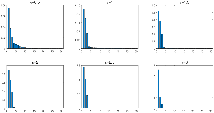
We sample $800$ points $\{(x^{\prime}_{i},y^{\prime}_{i},z^{\prime}_{i})\}_{i=1}^{800}$ uniformly on the surface. Let $R$ be an orthogonal matrix of $\mathbb{R}^{3}$. We rotate the surface by using $R$, i.e. we get $800$ points $\{(x^{\prime\prime}_{i},y^{\prime\prime}_{i},z^{\prime\prime}_{i})\}_{i=1}^{800}$ where $\begin{bmatrix}x^{\prime\prime}_{i}\\ y^{\prime\prime}_{i}\\ z^{\prime\prime}_{i}\end{bmatrix}=R\begin{bmatrix}x^{\prime}_{i}\\ y^{\prime}_{i}\\ z^{\prime}_{i}\end{bmatrix}$. Hence, $\iota(x_{i})=(0,\cdots,0,x^{\prime\prime}_{i},y^{\prime\prime}_{i},z^{\prime\prime}_{i},0,\cdots,0)\in\mathbb{R}^{30}$ ($x^{\prime\prime}_{i}$, $y^{\prime\prime}_{i}$, and $z^{\prime\prime}_{i}$ are the $14$th, $15$th, and $16$th coordinates, respectively) is a point on a surface of the ellipsoid $\iota(M)$ in $\mathbb{R}^{30}$. Suppose $\{\eta_{i}\}_{i=1}^{800}$ are i.i.d samples from $\mathcal{N}(0,\sigma^{2}I_{30\times 30})$ where $\sigma=0.05$. Then $\textbf{y}_{i}=\iota(x_{i})+\eta_{i}$ is a noisy data point around the submanifold $\iota(M)$ in $\mathbb{R}^{30}$. We choose the bandwidths $\epsilon=0.3,0.4,0.5,0.6$ and find $\{\bar{\lambda}_{\epsilon,i}\}_{i=1}^{30}$ by using $\{\iota(x_{i})\}_{i=1}^{800}$. We show the plot of $\{\bar{\lambda}_{\epsilon,i}\}_{i=1}^{30}$ for different $\epsilon$ in Fig 12 . We can see that there are two large eigenvalues. In other words, for this example, when there is no noise, the eigenvalues of the local covariance matrices constructed from $\{\iota(x_{i})\}_{i=1}^{800}$ are sufficient to determine the dimension of the underlying manifold.

Figure 12. We choose the bandwidths $\epsilon=0.3,0.4,0.5,0.6$ and find $\{\bar{\lambda}_{\epsilon,i}\}_{i=1}^{30}$ by using $\{\iota(x_{i})\}_{i=1}^{800}$. In the above plots, the horizontal axis indicates the $i=1,\cdots,30$ and the vertical axis indicates the value of corresponding $\bar{\lambda}_{\epsilon,i}$.

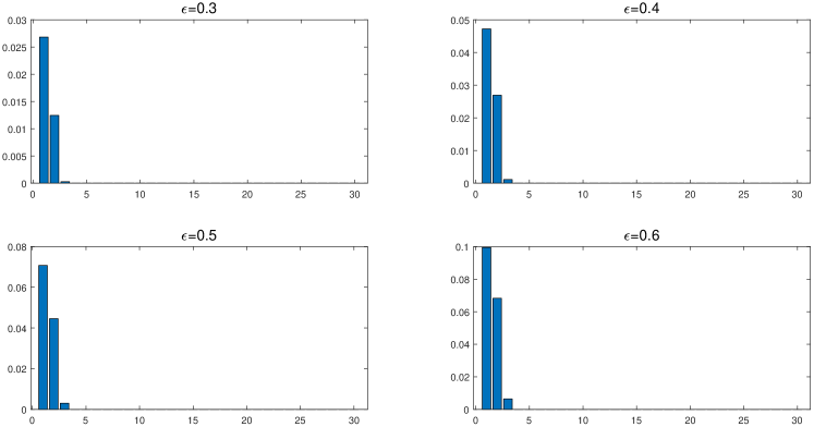
Next, we choose the bandwidths $\{\epsilon=0.1\ell\}_{\ell=1}^{30}$ and find $\{\bar{\lambda}_{\epsilon,i}\}_{i=1}^{30}$ by using $\{\textbf{y}_{i}\}_{i=1}^{800}$. We show the plot of $\{\bar{\lambda}_{\epsilon,i}\}_{i=1}^{30}$ for $\epsilon=0.5,1,\cdots,3$ in Fig 13 . Due to the noise, we cannot determine the dimension of $\iota(M)$ correctly by using the eigenvalues of the local covariance matrices constructed from $\{\textbf{y}_{i}\}_{i=1}^{800}$.

Figure 13. For $\{\epsilon=0.1\ell\}_{\ell=1}^{30}$, we find $\{\bar{\lambda}_{\epsilon,i}\}_{i=1}^{30}$ by using $\{\textbf{y}_{i}\}_{i=1}^{800}$. We plot $\{\bar{\lambda}_{\epsilon,i}\}_{i=1}^{30}$ for $\epsilon=0.5,1,\cdots,3$. In the above plots, the horizontal axis indicates $i=1,\cdots,30$ and the vertical axis indicates the value of the corresponding $\bar{\lambda}_{\epsilon,i}$ .

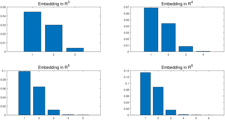
The robustness of diffusion map to noise is discussed in [12, 27, 11, 8]. Based on the description of the algorithm in Appendix E, we construct the normalized graph Laplacian $L\in\mathbb{R}^{n\times n}$ by using the kernel $k(\textbf{y},\textbf{y}^{\prime})=\exp(-\frac{\|\textbf{y}-\textbf{y}^{\prime}\|^{2}_{\mathbb{R}^{D}}}{\epsilon_{DM}^{2}})$ and the noisy data points $\{\textbf{y}_{i}\}_{i=1}^{800}$. We choose $\epsilon_{DM}=2$ and let $(\mu_{j},V_{j})_{j=0}^{n-1}$ be the eigenpairs of $-L$ with $\mu_{0}\leq\mu_{1}\leq\cdots,\leq\mu_{n-1}$ and $V_{i}$ normalizing in $\ell^{2}$. We reconstruct the noisy data points $\{\textbf{y}_{i}\}_{i=1}^{800}$ in $\mathbb{R}^{2+j}$ by using $(V_{1},\cdots,V_{2+j})\in\mathbb{R}^{800\times(2+j)}$ and denote these data points in $\mathbb{R}^{2+j}$ as $\mathcal{X}_{j}$ for $j=1,\cdots,4$. For each $j=1,\cdots,4$, the diffusion map $(V_{1},\cdots,V_{2+j})$ can be regarded as an approximation of a discretization of an embedding of $\iota(M)$ into $\mathbb{R}^{2+j}$ over the clean data point $\{\iota(x_{i})\}_{i=1}^{800}$ on $\iota(M)$. Hence, $\mathcal{X}_{j}$ are the samples around an embedded submanifold $N_{j}$ in $\mathbb{R}^{2+j}$ homeomorphic to $M$. The dimension of $M$ is the same as the dimension of $N_{j}$. For each $j=1,\cdots,4$, we construct the local covariance matrices by using $\mathcal{X}_{j}$ with $\epsilon=0.3+0.1j$ and calculate $\{\bar{\lambda}^{j}_{\epsilon,i}\}_{i=1}^{2+j}$. We plot $\{\bar{\lambda}^{j}_{\epsilon,i}\}_{i=1}^{2+j}$ for each $j$ in Figure 14. We can see that in each plot there are $2$ large eigenvalues. Therefore, the dimension of the underlying manifold $N_{j}$ and the dimension of $M$ are $2$.

Figure 14. $\mathcal{X}_{1},\cdots,\mathcal{X}_{4}$ constructed by diffusion map are the samples around the embeddings of $M$ in $\mathbb{R}^{3},\cdots,\mathbb{R}^{6}$, respectively. For each $j=1,\cdots,4$, we construct the local covariance matrices by using $\mathcal{X}_{j}$ with $\epsilon=0.3+0.1j$ and calculate $\{\bar{\lambda}^{j}_{\epsilon,i}\}_{i=1}^{2+j}$. We plot $\{\bar{\lambda}^{j}_{\epsilon,i}\}_{i=1}^{2+j}$ for each $j$. The top two plots correspond to $j=1,2$. The bottom two plots correspond to $j=3,4$. In the above plots, the horizontal axis indicates $i=1,\cdots,2+j$ and the vertical axis indicates the value of the corresponding $\bar{\lambda}^{j}_{\epsilon,i}$ .

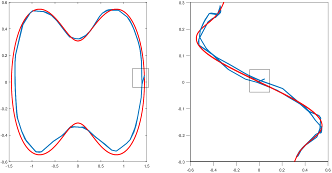
Appendix G Comparison of MrGap with principal graph method on Cassani Oval

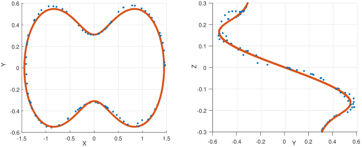
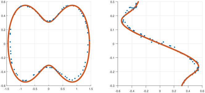
We compare the performance of MrGap on the noisy samples from the Cassini Oval $\iota(M)$ described in subsection 4.1 with the principal graph method of [21]. The principal graph method treats the data as vertices of a weighted graph and solves a minimization problem involving a number of nearest neighbors $nn$ and tuning parameters $\sigma_{p}$, $\gamma_{p}$ and $\lambda_{p}$. Recall that the Cassini Oval data set $\mathcal{Y}$ consists of $102$ noisy points near the curve and $\mathcal{Y}_{true}$ consists of $10^{5}$ points on the curve for us to estimate the GRMSE. $\mathcal{X}_{1}$ is the denoised output of the MrGap with $GRMSE(\mathcal{X}_{1},\mathcal{Y}_{true})=0.0224$. We plot $\mathcal{X}_{1}$ and $\mathcal{Y}_{true}$ in Figure 15. For the principal graph method, we choose $nn=5$, $\sigma_{p}=0.01$, $\gamma_{p}=0.5$ and $\lambda_{p}=1$ based on the suggestion in the code. We iterate the algorithm for $20$ times to acquire $102$ denoised data points $\mathcal{X}_{p}$, obtaining $GRMSE(\mathcal{X}_{p},\mathcal{Y}_{true})=0.0322$, which is 44% higher than $GRMSE(\mathcal{X}_{1},\mathcal{Y}_{true})$. We plot $\mathcal{X}_{p}$ and $\mathcal{Y}_{true}$ in Figure 16. The principal graph algorithm generates a curve which fits $\mathcal{Y}$. We plot the curve and $\mathcal{Y}_{true}$ in Figure 17. In the MrGap algorithm, we glue charts together by applying GP to construct a smooth manifold. However, in the principal graph method, there may be non smoothness generated as indicated in Figure 17.

Figure 15. $\mathcal{X}_{1}$ contains $102$ denoised points by the MrGap algorithm. The left and the right panels show the XY plot and YZ plot of $\mathcal{X}_{1}$ and $\mathcal{Y}_{true}$ respectively. The blue points are $\mathcal{X}_{1}$ and the red points are $\mathcal{Y}_{true}$. We use $\mathcal{Y}_{true}$ to estimate the GRMSE from samples to $\iota(M)$ with $GRMSE(\mathcal{X}_{1},\mathcal{Y}_{true})=0.0224$.

Figure 16. $\mathcal{X}_{p}$ contains $102$ denoised points on the Cassani Oval $\iota(M)$ by the principal graph algorithm. The left and the right panels show the XY plot and YZ plot of $\mathcal{X}_{p}$ and $\mathcal{Y}_{true}$ respectively. The blue points are $\mathcal{X}_{p}$ and the red points are $\mathcal{Y}_{true}$. We use $\mathcal{Y}_{true}$ to estimate the GRMSE from samples to $\iota(M)$ with $GRMSE(\mathcal{X}_{p},\mathcal{Y}_{true})=0.0322$.

Figure 17. The blue curve is the curve which fits the noisy data set $\mathcal{Y}$ by applying the principal graph algorithm. The red points are $\mathcal{Y}_{true}$. The left and the right panels show the XY plot and YZ plot of the fitting curve and $\mathcal{Y}_{true}$ respectively. The fitting curve is not smooth at the indicated position.

References

- [1] Eddie Aamari and Clément Levrard. Nonasymptotic rates for manifold, tangent space and curvature estimation. The Annals of Statistics, 47(1):177–204, 2019.
- [2] Yariv Aizenbud and Barak Sober. Non-parametric estimation of manifolds from noisy data. arXiv preprint arXiv:2105.04754, 2021.
- [3] Mikhail Belkin and Partha Niyogi. Laplacian eigenmaps for dimensionality reduction and data representation. Neural computation, 15(6):1373–1396, 2003.
- [4] Jean-Daniel Boissonnat, André Lieutier, and Mathijs Wintraecken. The reach, metric distortion, geodesic convexity and the variation of tangent spaces. Journal of applied and computational topology, 3(1):29–58, 2019.
- [5] Jeff Calder, Nicolas Garcia Trillos, and Marta Lewicka. Lipschitz regularity of graph Laplacians on random data clouds. SIAM Journal on Mathematical Analysis, 54(1):1169–1222, 2022.
- [6] Xiuyuan Cheng and Nan Wu. Eigen-convergence of Gaussian kernelized graph Laplacian by manifold heat interpolation. Applied and Computational Harmonic Analysis, 61:132–190, 2022.
- [7] Ronald R Coifman and Stéphane Lafon. Diffusion maps. Applied and Computational Harmonic Analysis, 21(1):5–30, 2006.
- [8] Xiucai Ding and Hau-Tieng Wu. Impact of signal-to-noise ratio and bandwidth on graph Laplacian spectrum from high-dimensional noisy point cloud. arXiv preprint arXiv:2011.10725, 2020.
- [9] Manfredo P Do Carmo. Riemannian geometry. Springer Science & Business Media, 2013.
- [10] David B. Dunson, Hau-Tieng Wu, and Nan Wu. Spectral convergence of graph Laplacian and heat kernel reconstruction in from random samples. Applied and Computational Harmonic Analysis, 55:282–336, 2021.
- [11] David B. Dunson, Hau-Tieng Wu, and Nan Wu. Graph based Gaussian processes on restricted domains. Journal of the Royal Statistical Society: Series B (Statistical Methodology), 84(2):414–439, 2022.
- [12] Noureddine El Karoui and Hau-Tieng Wu. Graph connection Laplacian methods can be made robust to noise. The Annals of Statistics, 44(1):346–372, 2016.
- [13] Herbert Federer. Curvature measures. Transactions of the American Mathematical Society, 93(3):418–491, 1959.
- [14] Charles Fefferman, Sergei Ivanov, Yaroslav Kurylev, Matti Lassas, and Hariharan Narayanan. Fitting a putative manifold to noisy data. 75:688–720, 2018.
- [15] Charles Fefferman, Sergei Ivanov, Matti Lassas, and Hariharan Narayanan. Fitting a manifold of large reach to noisy data. arXiv preprint arXiv:1910.05084, 2019.
- [16] Christopher Genovese, Marco Perone-Pacifico, Isabella Verdinelli, and Larry Wasserman. Minimax manifold estimation. Journal of Machine Learning Research, 13(43):1263–1291, 2012.
- [17] Trevor Hastie and Werner Stuetzle. Principal curves. Journal of the American Statistical Association, 84(406):502–516, 1989.
- [18] John H Kalivas. Two data sets of near infrared spectra. Chemometrics and Intelligent Laboratory Systems, 37(2):255–259, 1997.
- [19] Daniel N Kaslovsky and François G Meyer. Non-asymptotic analysis of tangent space perturbation. Information and Inference: a Journal of the IMA, 3(2):134–187, 2014.
- [20] Slav Kirov and Dejan Slepčev. Multiple penalized principal curves: analysis and computation. Journal of Mathematical Imaging and Vision, 59(2):234–256, 2017.
- [21] Qi Mao, Li Wang, Ivor W Tsang, and Yijun Sun. Principal graph and structure learning based on reversed graph embedding. IEEE Transactions on Pattern Analysis and Machine Intelligence, 39(11):2227–2241, 2016.
- [22] Kun Meng and Ani Eloyan. Principal manifold estimation via model complexity selection. Journal of the Royal Statistical Society: Series B (Statistical Methodology), 83(2):369–394, 2021.
- [23] James R Munkres. Analysis on manifolds. CRC Press, 2018.
- [24] Partha Niyogi, Stephen Smale, and Shmuel Weinberger. Finding the homology of submanifolds with high confidence from random samples. Discrete & Computational Geometry, 39(1-3):419–441, 2008.
- [25] Carl Edward Rasmussen. Gaussian processes in machine learning. In Summer School on Machine Learning, pages 63–71. Springer, 2003.
- [26] Sam T Roweis and Lawrence K Saul. Nonlinear dimensionality reduction by locally linear embedding. Science, 290(5500):2323–2326, 2000.
- [27] Chao Shen and Hau-Tieng Wu. Scalability and robustness of spectral embedding: landmark diffusion is all you need. arXiv preprint arXiv:2001.00801, 2020.
- [28] Amit Singer and H-T Wu. Vector diffusion maps and the connection Laplacian. Communications on Pure and Applied Mathematics, 65(8):1067–1144, 2012.
- [29] Alexander Smola, Sebastian Mika, Bernhard Schölkopf, Robert Williamson, et al. Regularized principal manifolds. Journal of Machine Learning Research, 1:179–209, 2001.
- [30] Joshua B Tenenbaum, Vin De Silva, and John C Langford. A global geometric framework for nonlinear dimensionality reduction. Science, 290(5500):2319–2323, 2000.
- [31] Laurens Van der Maaten and Geoffrey Hinton. Visualizing data using t-SNE. Journal of Machine Learning Research, 9(11):2579–2605, 2008.
- [32] Per Åke Wedin. On angles between subspaces of a finite dimensional inner product space. In Matrix Pencils, pages 263–285. Springer, 1983.
- [33] Hau-Tieng Wu and Nan Wu. Think globally, fit locally under the manifold setup: Asymptotic analysis of locally linear embedding. The Annals of Statistics, 46(6B):3805–3837, 2018.
- [34] Hau-Tieng Wu and Nan Wu. When locally linear embedding hits boundary. arXiv preprint arXiv:1811.04423, 2018.
- [35] Hau-Tieng Wu and Nan Wu. Strong uniform consistency with rates for kernel density estimators with general kernels on manifolds. Information and Inference: A Journal of the IMA, 11(2):781–799, 2021.