Abstract

We introduce a kernel estimator, to the tail index of a right-censored Pareto-type distribution, that generalizes Worms’s one (Worms and Worms, 2014) in terms of weight coefficients. Under some regularity conditions, the asymptotic normality of the proposed estimator is established. In the framework of the second-order condition, we derive an asymptotically bias-reduced version to the new estimator. Through a simulation study, we conclude that one of the main features of the proposed kernel estimator is its smoothness contrary to Worms’s one, which behaves, rather erratically, as a function of the number of largest extreme values. As expected, the bias significantly decreases compared to that of the non-smoothed estimator with however a slight increase in the mean squared error.

Keywords: asymptotic distributions; heavy-tailed estimation; kernel estimation; right-censored data.

AMS 2010 Subject Classification: Primary 62G32; 62G30; secondary 60G70; 60F17.

${}^{\text{*}}$Corresponding author: ah.necir@univ-biskra.dz
E-mail address:
l.soltane@univ-biskra.dz (L. Soltane)

1. Introduction

1.1. A review of the tail index estimation

Let $X_{1},X_{2},...,X_{n}$ be independent and identically distributed (iid) of non-negative random variables (rv’s) as $n$ copies of a rv $X,$ defined over some probability space $\left(\Omega,\mathcal{A},\mathbf{P}\right),$ with cumulative distribution function (cdf) $F.\$We assume that the distribution tail $\overline{F}:=1-F$ is regularly varying at infinity, with index $\left(-1/\gamma_{1}\right),$ notation: $\overline{F}\in\mathcal{RV}_{\left(-1/\gamma_{1}\right)},$ that is

$$\lim_{t\rightarrow\infty}\frac{\overline{F}\left(tx\right)}{\overline{F}\left(t\right)}=x^{-1/\gamma_{1}},\text{ for any }x>0,$$ (1.1)

where $\gamma_{1}>0$ is called the shape parameter or the tail index or the extreme value index (EVI). It plays a very crucial role in the analysis of extremes as it governs the thickness of the distribution right-tail. The most popular estimator of $\gamma_{1}$ is Hill’s estimator Hill (1975) defined by

$$\widehat{\gamma}_{1,k}^{\left(H\right)}:=\frac{1}{k}{\displaystyle\sum\limits_{i=1}^{k}}\log\frac{X_{n-i+1:n}}{X_{n-k:n}}={\displaystyle\sum\limits_{i=1}^{k}}\frac{i}{k}\log\frac{X_{n-i+1:n}}{X_{n-i:n}},$$ (1.2)

where $X_{1:n}\leq...\leq X_{n:n}$ denote the order statistics pertaining to the sample $\left(X_{1},...,X_{n}\right)$ and $k=k_{n}$ is an integer sequence satisfying $1<k<n,$ $k\rightarrow\infty$ and $k/n\rightarrow 0$ as $n\rightarrow\infty.$ The discrete character and non-stability of Hill’s estimator present major drawbacks. Indeed, adding a single large-order statistic in the calculation of the estimator, that is, increasing $k$ by $1,$ may deviate from the true value of the estimate substantially. Thus, the plotting of this estimator as a function of the upper order statistics often gives a zig-zag figure (see Figure $\ref{Figure1}).$

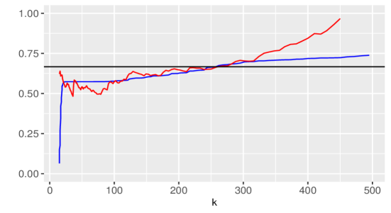
Figure 1.1. Ploting both Hill’s (red line) and CDM’s (blue line) tail index estimators, as function of $k$ upper order statistics, for a Pareto-type distribution.

To overcome this issue, Csörgő et al. (1985) introduced more general weighs instead of the natural one $i/k$ that appears in the second formula of $\widehat{\gamma}_{1,k}^{\left(H\right)},$ to define the following kernel estimator

$$\widehat{\gamma}_{1,k}^{\left(CDM\right)}\left(K\right):=\sum_{i=1}^{k}\frac{i}{k+1}K\left(\frac{i}{k+1}\right)\log\frac{X_{n-i+1:n}}{X_{n-i:n}},$$

where $K$ is a kernel function satisfying the following assumptions:

• $\left[A1\right]$ is non increasing and right-continuous on $\mathbb{R}.$

• $\left[A2\right]$ $K\left(s\right)=0$ for $s\notin\left(0,1\right]$ and $K\left(s\right)\geq 0$ for $s\in\left(0,1\right].$

• $\left[A3\right]$ $\int_{\mathbb{R}}K\left(s\right)ds=1.$

• $\left[A4\right]$ $K$ and its first and second Lebesgue derivatives $K^{\prime}$ and $K^{\prime\prime}$ are bounded.

The commonly used kernel functions are: the indicator kernel $K_{1}:=\mathbf{1}\left\{\left[0,1\right)\right\},$ the biweight, triweight and quadweight kernels respectively defined on $0\leq s<1$ by

$$K_{2}\left(s\right):=\frac{15}{8}\left(1-s^{2}\right)^{2},\text{ }K_{3}\left(s\right):=\frac{35}{16}\left(1-s^{2}\right)^{3},\text{ }K_{4}\left(s\right):=\frac{315}{128}\left(1-s^{2}\right)^{4},$$ (1.3)

and zero elsewhere, where $\mathbf{1}\left\{A\right\}$ stands for the indicator function of a set $A.$ Note that the indicator kernel $K_{1}$ corresponds to the weigh coefficients of a closely related tail index estimator to Hill’s one $\widehat{\gamma}_{1,k}^{\left(H\right)}.$ The nice properties of the kernel estimator $\widehat{\gamma}_{1,k}^{\left(CDM\right)}\left(K\right)$ are the smoothness and the stability, contrary to Hill’s one which rather exhibits fluctuations along the range of upper extreme values. Thanks to these features, the exact choice of $k$ to be used in the kernel estimator becomes not as crucial as that in Hill’s one (see, e.g., Groeneboom et al., 2003). For an overview of the kernel estimates of the tail index for complete data, one refers to Hüsler et al. (2006), Ciuperca and Mercadier (2010), Goregebeur et al. (2010) and Caeiro and Henriques-Rodrigues (2019) and references therein. Motivated by the qualities of this estimation method, recently Benchaira et al. (2016) proposed a kernel estimator of the tail index for randomly truncated data and established its asymptotic normality. To the best of our knowledge, when the data are randomly censored, this estimation approach is not yet addressed in the extreme value literature. In the following section we present a review of the existing tail index estimators and then propose kernel estimators to $\gamma_{1}$ for censored data.

2. Review of tail index estimation for censored data

In the analysis of lifetime, reliability or insurance data, the observations are usually randomly censored. In other words, in many real situations the variable of interest $X$ is not always available. An appropriate way to model this matter, is to introduce a non-negative rv $Y,$ called censoring rv, independent of $X$ and then to consider the rv $Z:=\min\left(X,Y\right)$ and the indicator variable $\delta:=\mathbf{1}\left\{X\leq Y\right\},$ which determines whether or not $X$ has been observed. The cdf’s of $Y$ and $Z$ will be denoted by $G$ and $H$ respectively. The analysis of extreme values of randomly censored data is a new research topic to which Reiss and Thomas (2007) made a very brief reference, in Section 6.1, as a first step but with no asymptotic results. Considering Hall’s model (Hall, 1982), Beirlant et al. (2007) proposed estimators for the EVI and high quantiles and discussed their asymptotic properties, when the data are censored by a deterministic threshold. Einmahl et al. (2008) adapted various EVI estimators to the case where data are censored by a random threshold and proposed a unified method to establish their asymptotic normality. In this context, the censoring distribution is assumed to be regularly varying too, that is $\overline{G}\in\mathcal{RV}_{\left(-1/\gamma_{2}\right)},$ for some $\gamma_{2}>0.$ By virtue of the independence of $X$ and $Y,$ we have $\overline{H}\left(x\right)=\overline{F}\left(x\right)\overline{G}\left(x\right)$ and therefore $\overline{H}\in\mathcal{RV}_{\left(-1/\gamma\right)},$ with $\gamma:=\gamma_{1}\gamma_{2}/\left(\gamma_{1}+\gamma_{2}\right).$ We also assume that both $\overline{F}$ and $\overline{G}$ satisfy the second-order condition of regularly varying functions:

$$\overline{F}\left(x\right) =C_{1}x^{-1/\gamma_{1}}\left(1+D_{1}x^{-\beta_{1}}\left(1+o\left(1\right)\right)\right),\text{ as }x\rightarrow\infty,$$ (2.4)

$$\overline{G}\left(y\right) =C_{2}y^{-1/\gamma_{2}}\left(1+D_{2}y^{-\beta_{2}}\left(1+o\left(1\right)\right)\right),\text{ as }y\rightarrow\infty,$$ (2.5)

where $\beta_{1},\beta_{2},C_{1},C_{2}$ are positive constants and $D_{1},D_{2}$ are real constants. The parameters $\tau_{i}:=-\beta_{i}\gamma_{i}<0,$ $i=1,2$ called the second-order parameters corresponding to cdf’s $F$ and $G$ respectively. This class of cdf’s is known by Hall’s models which contains the most usual Pareto-type cdf’s, namely Burr, Fréchet, GEV, GPD, Student, etc. The previous two conditions together imply that

$$\overline{H}\left(z\right)=Cz^{-1/\gamma}\left(1+D_{\ast}z^{-\beta_{\ast}\gamma}\left(1+o\left(1\right)\right)\right),\text{ as }z\rightarrow\infty,$$ (2.6)

where $C:=C_{1}C_{2},$ $\beta_{\ast}:=\min\left(\beta_{1},\beta_{2}\right)$ and

$$D_{\ast}:=D_{1}\mathbf{1}\left\{\beta_{1}<\beta_{2}\right\}+D_{2}\mathbf{1}\left\{\beta_{1}>\beta_{2}\right\}+\left(D_{1}+D_{2}\right)\mathbf{1}\left\{\beta_{1}=\beta_{2}\right\}.$$

Let $\left\{\left(Z_{1},\delta_{1}\right),...,\left(Z_{n},\delta_{n}\right)\right\}$ be a sample from the couple of rv’s $\left(Z,\delta\right)$ and let $Z_{1:n}\leq...\leq Z_{n:n}$ denote the order statistics pertaining to $\left(Z_{1},...,Z_{n}\right).$ If we denote the concomitant of the $i$th order statistic by $\delta_{\left(i\right)}$ (i.e. $\delta_{\left(i\right)}=\delta_{j}$ if $Z_{i:n}=Z_{j}),$ then the adapted Hill estimator of the tail index $\gamma_{1}$ is defined by

$$\widehat{\gamma}_{1,k}^{\left(EFG\right)}:=\frac{\widehat{\gamma}_{k}^{\left(H\right)}}{\widehat{p}_{k}},$$ (2.7)

where $\widehat{\gamma}_{k}^{\left(H\right)}$ is Hill’s estimator of the tail index $\gamma$ and $\widehat{p}_{k}:=k^{-1}\sum\limits_{i=1}^{k}\delta_{\left(n-i+1\right)}$ denotes the estimator of asymptotic proportion of non-censored observations in the tail given by

$$p:=\frac{\gamma}{\gamma_{1}}=\frac{\gamma_{2}}{\gamma_{1}+\gamma_{2}},$$ (2.8)

which is the limit, as $z\rightarrow\infty,$ of function

$$p\left(z\right):=\mathbf{P}\left(\delta=1\mid Z=z\right).$$ (2.9)

Asymptotic representations both to $\widehat{\gamma}_{k}^{\left(H\right)}$ and $\widehat{p}_{k}$ in terms of Brownian bridges processes, given by Brahimi et al. (2015), leading to the asymptotic normality of $\widehat{\gamma}_{1,k}^{\left(EFG\right)}$ under the usual second-order conditions of regularly varying functions. In this context, the estimation of the conditional tail index is addressed in Ndao et al. (2014), Ndao et al. (2016), Stupfler (2016) and Goegebeur et al. (2019). Recently Stupfler (2019) assumed that the censoring and the censored rv’s are dependant and proposed an estimation procedure to $\gamma_{1}.$

By using a Kaplan-Meier integral Beirlant et al. (2019) proposed in new estimator to $\gamma_{1}$ defined by

$$\widehat{\gamma}_{1,k}^{\left(W\right)}:=\sum_{j=2}^{k}\frac{\overline{F}_{n}^{KM}\left(Z_{n-j+1:n}\right)}{\overline{F}_{n}^{KM}\left(Z_{n-k:n}\right)}\log\frac{Z_{n-j+1:n}}{Z_{n-j:n}},$$ (2.10)

where

$$\overline{F}_{n}^{KM}\left(t\right):=\left\{\begin{array}[c]{lc}\prod\limits_{i=1}^{n}\left(1-\dfrac{\delta_{\left(i\right)}}{n-i+1}\right)^{\mathbf{1}\left\{Z_{i:n}\leq t\right\}}&\text{if }t<Z_{n:n}\vskip 6.0pt plus 2.0pt minus 2.0pt\\ 0&\text{otherwise}\end{array}\right.,$$

denotes the well-known Kaplan-Meier product-limit estimator (Kaplan and Meier, 1958) of the underlying cdf $F.$ Actually $\widehat{\gamma}_{1,k}^{\left(W\right)}$ is a slight modification of the tail index estimator

$$\widetilde{\gamma}_{1,k}^{\left(W\right)}:=\sum_{j=1}^{k}\frac{\overline{F}_{n}^{KM}\left(Z_{n-j:n}\right)}{\overline{F}_{n}^{KM}\left(Z_{n-k:n}\right)}\log\frac{Z_{n-j+1:n}}{Z_{n-j:n}},$$

first given by Worms and Worms (2014). We showed in Proposition 6.2 that the increments

$$\frac{\overline{F}_{n}^{KM}\left(Z_{n-j:n}\right)}{\overline{F}_{n}^{KM}\left(Z_{n-k:n}\right)}-\frac{\overline{F}_{n}^{KM}\left(Z_{n-j+1:n}\right)}{\overline{F}_{n}^{KM}\left(Z_{n-k:n}\right)},\text{ }j=1,...,k,$$

are negligible (in probability) for all large $n,$ this means that the estimation of $\overline{F}_{n}^{KM}\left(Z_{n-j:n}\right)/\overline{F}_{n}^{KM}\left(Z_{n-k:n}\right)$ by $\overline{F}_{n}^{KM}\left(Z_{n-j+1:n}\right)/\overline{F}_{n}^{KM}\left(Z_{n-k:n}\right)$ is well justified. The authors also showed that for a suitable sequence of integer $k,$ we have

$$\sqrt{k}\left(\widehat{\gamma}_{1,k}^{\left(W\right)}-\gamma_{1}\right)\overset{\mathcal{D}}{\rightarrow}\mathcal{N}\left(\lambda m,p\gamma_{1}^{2}/\left(2p-1\right)\right),\text{ as }n\rightarrow\infty,$$ (2.11)

for some real constants $\lambda,$ where $m:=-\mathbf{1}\left\{\beta_{1}\leq\beta_{2}\right\}\gamma^{2}\beta_{1}D_{1}C^{-\gamma\beta_{1}}p^{-1}\left(1+\beta_{1}\gamma/p\right)^{-1},$ provided that $p>1/2$ which is equivalent to $\gamma_{1}<\gamma_{2}.$ In the real-life applications, the latter assumption may be realizable. Indeed, Beirlant et al. (2018) gave an application to insurance data and claim that exhibits heavy-tail and part of these can be considered to satisfy the $p>1/2.$ Through simulations, Worms and Worms (2014) showed that $\widehat{\gamma}_{1,k}^{\left(W\right)}$ performs better than the adapted Hill estimator $\widehat{\gamma}_{1,k}^{\left(EFG\right)},$ in the weak-censoring case $p>1/2,$ both in term of bias and mean squared error (MSE). However the estimator exhibits a slightly high bias which is natural when one deals with Hill-type estimators. Instead of Kaplan-Meier approach, Brahimi et al. (2016) proposed another asymptotically normal estimator of $\gamma_{1}$ close to $\widehat{\gamma}_{1,k}^{\left(W\right)}$ that is based of the Nelson-Aalen nonparametric estimator (Nelson, 1972), which seems to have a slightly lower bias compared with that of $\widehat{\gamma}_{1,k}^{\left(W\right)}.$ As expected, the asymptotic biases and variances corresponding to the two estimators meet.

Recently Bladt et al. (2021) proposed the following class of kernel estimators defined by

$$\widehat{\gamma}_{1,k}^{\left(BAB\right)}\left(\mathcal{K}\right):=\frac{1}{k}\sum_{i=1}^{k}\mathcal{K}\left(\frac{i}{k+1},\widehat{p}_{k}\right)\frac{1}{\log\left(\left(k+1\right)/i\right)}\log\frac{Z_{n-i+1:n}}{Z_{n-k:n}},$$ (2.12)

where $\widehat{p}_{k}$ is given in $\left(\ref{AH}\right)$ and $\mathcal{K}$ is a positive kernel satisfying $p\int_{0}^{1}\mathcal{K}\left(s,p\right)du=1,$ for $p\in\left(0,1\right].$ The particular kernel functions used by the authors are:

$$\mathcal{K}_{0}\left(s,p\right):=\frac{1}{p}\log\frac{1}{s},\text{ }\mathcal{K}_{1}\left(s,p\right):=s^{p-1},\text{ }\mathcal{K}_{2}\left(s,p\right):=\frac{s^{p-1}-1}{1-p}.$$ (2.13)

Since $\widehat{\gamma}_{1,k}^{\left(BAB\right)}\left(\mathcal{K}_{0}\right)\equiv\widehat{\gamma}_{1,k}^{\left(EFG\right)},$ then this kernel estimator can be viewed as a generalization of$\ \widehat{\gamma}_{1,k}^{\left(EFG\right)},$ in terms of weight coefficients. As mentioned in their paper, Worms’s estimator $\widehat{\gamma}_{1,k}^{\left(W\right)}$ does not fall into this framework, but it simplified version $\widehat{\gamma}_{1,k}^{\left(BAB\right)}\left(\mathcal{K}\right)$ does. In their simulation study, Bladt et al. (2021) pointed out that the MSE characteristics of the estimator $\widehat{\gamma}_{1,k}^{\left(BAB\right)}\left(\mathcal{K}_{2}\right)$ are quite comparable to those of $\widehat{\gamma}_{1,k}^{\left(W\right)}.$ Overall, however, $\widehat{\gamma}_{1,k}^{\left(W\right)}$ performs better $\widehat{\gamma}_{1,k}^{\left(BAB\right)}\left(\mathcal{K}\right)$ in terms of bias for the three kernel functions. The asymptotic normality of this estimator is established by considering both weak and strong censoring cases $\left(\text{i.e. }0<p\leq 1\right).$ We can summarize the features of BAB’s estimator in two points: its smoothness compared with $\widehat{\gamma}_{1,k}^{\left(EFG\right)}$ and its asymptotic normality which is hold for all $0<p\leq 1$ however that of Worms’s one is limited only to the interval $p>1/2.$

In the following section we introduce a new kernel estimator for the tail index $\gamma_{1}$ that generalizes $\widehat{\gamma}_{1,k}^{\left(W\right)}$ is the sense that the two estimators coincide for the indicator function $K_{1}.$ In other terms, this new kernel estimator is a generalization of CDM’s estimator $\widehat{\gamma}_{1,k}^{\left(CDM\right)}\left(K\right)$ to the case of censored data.

2.1. A new kernel estimator for $\gamma_{1}$

By using Potter’s inequalities, see e.g. Proposition B.1.10 in de Haan and Ferreira (2006), to the regularly varying function $F$ together with assumptions $[A1]-[A4],$ Benchaira et al. (2016) showed that

$$\lim_{u\rightarrow\infty}\int_{u}^{\infty}g_{K}^{\prime}\left(\frac{\overline{F}\left(x\right)}{\overline{F}\left(u\right)}\right)\log\frac{x}{u}d\frac{F\left(x\right)}{\overline{F}\left(u\right)}=\gamma_{1}\int_{0}^{\infty}K\left(x\right)dx=\gamma_{1},$$

where $g_{K}\left(x\right):=xK\left(x\right)$ and $g^{\prime}$ denotes the Lebesgue derivative of $g.$ Since $\overline{F}$ is continuous, then $\overline{F}\left(x\right)=\overline{F}\left(x^{-}\right),$ this allows us to write

$$\frac{\overline{F}\left(x\right)}{\overline{F}\left(u\right)}=\theta_{x,u}\frac{\overline{F}\left(x^{-}\right)}{\overline{F}\left(u\right)}+\left(1-\theta_{x,u}\right)\frac{\overline{F}\left(x\right)}{\overline{F}\left(u\right)},\text{ for }x>u,$$

for some arbitrary real number $0<\theta_{x,u}<1.$ Next we will see that, thanks to the mean value theorem, this formula provides us an estimation of the derivative $g^{\prime}$ in terrmes of an increment of function $g;$ see equation $\left(\ref{mv}\right)$ below. The notation $\psi\left(a^{-}\right):=\lim_{x\uparrow a}\psi\left(x\right)$ stands for the left-limit of a function $\psi\left(t\right)$ as $t$ approaches $a$ from the left. By letting $u=Z_{n-k:n}$ and substituting $F$ by Kaplan-Meier estimator $F_{n}^{KM},$ we derive a kernel estimator to the tail index $\gamma_{1}$ defined by

$$\widetilde{\gamma}_{1,k}\left(K\right):=\int_{Z_{n-k:n}}^{\infty}g_{K}^{\prime}\left(\mathcal{F}_{n}\left(x\right)\right)\log\left(\frac{x}{Z_{n-k:n}}\right)\frac{dF_{n}^{KM}\left(x\right)}{\overline{F}_{n}^{KM}\left(Z_{n-k:n}\right)},$$

where

$$\mathcal{F}_{n}\left(x\right):=\theta_{x,n}\frac{\overline{F}_{n}^{KM}\left(x^{-}\right)}{\overline{F}_{n}^{KM}\left(Z_{n-k:n}\right)}+\left(1-\theta_{x,n}\right)\frac{\overline{F}_{n}^{KM}\left(x\right)}{\overline{F}_{n}^{KM}\left(Z_{n-k:n}\right)},$$

and $\theta_{x,n}:=\theta_{x,Z_{n-k:n}}$ $\left(\text{arbitrary}\right).$ To rewrite the previous integral into a sum form, we use the following crucial equation: for a given functional $\phi\left(\cdot;F\right),$ we have

$$\int\phi\left(x;F\right)dF\left(x\right)=\int\frac{\phi\left(z;F\right)}{\overline{G}\left(z\right)}\left\{\overline{G}\left(z\right)dF\left(z\right)\right\}=\int\frac{\phi\left(z;F\right)}{\overline{G}\left(z\right)}dH^{1}\left(z\right),$$ (2.14)

where $H^{1}\left(z\right):=\mathbf{P}\left(Z\leq z,\delta=1\right)=\int_{0}^{z}\overline{G}\left(x\right)dF\left(x\right),$ see for instance Stute (1995). The empirical counterparts of integrals in $\left(\ref{eq}\right)$ are

$$\int\phi\left(x;F_{n}^{KM}\right)dF_{n}^{KM}\left(x\right)=\int\frac{\phi\left(z;F_{n}^{KM}\right)}{\overline{G}_{n}^{KM}\left(z^{-}\right)}dH_{n}^{1}\left(z\right),$$

where

$$\overline{G}_{n}^{KM}\left(t\right):=\left\{\begin{array}[c]{lc}{\displaystyle\prod\limits_{i=1}^{n}}\left(1-\dfrac{1-\delta_{\left(i\right)}}{n-i+1}\right)^{\mathbf{1}\left\{Z_{i:n}\leq t\right\}}&\text{if }t<Z_{n:n}\vskip 6.0pt plus 2.0pt minus 2.0pt\\ 0&\text{otherwise}\end{array}\right.,$$

denotes the Kaplan-Meire estimator of cdf $G$ and $H_{n}^{1}\left(z\right):=n^{-1}\sum\limits_{i=1}^{n}\mathbf{1}\left\{Z_{i}\leq z,\text{ }\delta_{i}=1\right\},$ is the empirical counterpart of the subdisribution function $H^{1}.$ We used $\overline{G}_{n}^{KM}\left(t^{-}\right)$ instead of $\overline{G}_{n}^{KM}\left(t\right)$ to avoid a division by zero, besides that $\overline{G}_{n}^{KM}\left(Z_{n:n}\right)=0.$ For convenience, we set

$$\phi_{n}\left(x;F\right):=\frac{1}{\overline{F}_{n}^{KM}\left(Z_{n-k:n}\right)}g_{K}^{\prime}\left(\mathcal{F}_{n}\left(x\right)\right)\log\frac{x}{Z_{n-k:n}}\mathbf{1}\left\{x>Z_{n-k:n}\right\}.$$

Thus, the kernel estimator $\widetilde{\gamma}_{1,k}\left(K\right)$ may be rewritten into

$$\int_{0}^{\infty}\phi_{n}\left(x;F_{n}^{KM}\right)dF_{n}\left(x\right)=\int_{0}^{\infty}\frac{\phi_{n}\left(z;F_{n}^{KM}\right)}{\overline{G}_{n}^{KM}\left(z^{-}\right)}dH_{n}^{1}\left(z\right),$$

which equals

$$\sum_{i=1}^{n}\frac{\mathbf{1}\left\{Z_{i:n}>Z_{n-k:n}\right\}}{\overline{F}_{n}^{KM}\left(Z_{n-k:n}\right)}\frac{\delta_{\left(i\right)}}{n\overline{G}_{n}^{KM}\left(Z_{i:n}^{-}\right)}g_{K}^{\prime}\left(\mathcal{F}_{n}\left(Z_{i:n}\right)\right)\log\frac{Z_{i:n}}{Z_{n-k:n}}.$$

$$=\sum_{i=n-k+1}^{n}\frac{\delta_{\left(i\right)}}{n\overline{F}_{n}^{KM}\left(Z_{n-k:n}\right)\overline{G}_{n}^{KM}\left(Z_{i-1:n}\right)}g_{K}^{\prime}\left(\mathcal{F}_{n}\left(Z_{i:n}\right)\right)\log\frac{Z_{i:n}}{Z_{n-k:n}},$$

where

$$\mathcal{F}_{n}\left(Z_{i:n}\right):=\theta_{i,n}\frac{\overline{F}_{n}^{KM}\left(Z_{i-1:n}\right)}{\overline{F}_{n}^{KM}\left(Z_{n-k:n}\right)}+\left(1-\theta_{i,n}\right)\frac{\overline{F}_{n}^{KM}\left(Z_{i:n}\right)}{\overline{F}_{n}^{KM}\left(Z_{n-k:n}\right)},$$

where $\left(\theta_{i,n}\right)_{1\leq i\leq k}$ is an arbitrary random sequence. By changing the index of summation $i$ to $n-j+1,$ yields

$$\widetilde{\gamma}_{1,k}\left(K\right)=\sum_{j=1}^{k}\frac{\delta_{\left(n-j+1\right)}}{n\overline{F}_{n}^{KM}\left(Z_{n-k:n}\right)\overline{G}_{n}^{KM}\left(Z_{n-j:n}\right)}g_{K}^{\prime}\left(\mathcal{F}_{n}\left(Z_{n-j+1:n}\right)\right)\log\frac{Z_{n-j+1:n}}{Z_{n-k:n}}.$$

We showed in Proposition 6.1 that

$$\frac{\delta_{\left(n-j+1\right)}}{n\overline{G}_{n}^{KM}\left(Z_{n-j:n}\right)}=\overline{F}_{n}^{KM}\left(Z_{n-j:n}\right)-\overline{F}_{n}^{KM}\left(Z_{n-j+1:n}\right),$$

therefore

$$\widetilde{\gamma}_{1,k}\left(K\right) =\sum_{j=1}^{k}\left\{\frac{\overline{F}_{n}^{KM}\left(Z_{n-j:n}\right)}{\overline{F}_{n}^{KM}\left(Z_{n-k:n}\right)}-\frac{\overline{F}_{n}^{KM}\left(Z_{n-j+1:n}\right)}{\overline{F}_{n}^{KM}\left(Z_{n-k:n}\right)}\right\}$$

$$\ \ \ \ \ \ \ \ \ \ \ \ \ \ \times g_{K}^{\prime}\left(\mathcal{F}_{n}\left(Z_{n-j+1:n}\right)\right)\log\frac{Z_{n-j+1:n}}{Z_{n-k:n}}.$$

In view of the mean value theorem, we may choose the sequence of constants $\theta_{j,n}$ so that

$$g_{K}^{\prime}\left(\mathcal{F}_{n}\left(Z_{n-j+1:n}\right)\right)=\frac{g_{K}\left(\frac{\overline{F}_{n}^{KM}\left(Z_{n-j:n}\right)}{\overline{F}_{n}^{KM}\left(Z_{n-k:n}\right)}\right)-g_{K}\left(\frac{\overline{F}_{n}^{KM}\left(Z_{n-j+1:n}\right)}{\overline{F}_{n}^{KM}\left(Z_{n-k:n}\right)}\right)}{\frac{\overline{F}_{n}^{KM}\left(Z_{n-j:n}\right)}{\overline{F}_{n}^{KM}\left(Z_{n-k:n}\right)}-\frac{\overline{F}_{n}^{KM}\left(Z_{n-j+1:n}\right)}{\overline{F}_{n}^{KM}\left(Z_{n-k:n}\right)}},$$ (2.15)

thus

$$\widetilde{\gamma}_{1,k}\left(K\right)=\sum_{j=1}^{k}\left\{g_{K}\left(\frac{\overline{F}_{n}^{KM}\left(Z_{n-j:n}\right)}{\overline{F}_{n}^{KM}\left(Z_{n-k:n}\right)}\right)-g_{K}\left(\frac{\overline{F}_{n}^{KM}\left(Z_{n-j+1:n}\right)}{\overline{F}_{n}^{KM}\left(Z_{n-k:n}\right)}\right)\right\}\log\frac{Z_{n-j+1:n}}{Z_{n-k:n}}.$$ (2.16)

Recall that $g_{K}\left(x\right)=xK\left(x\right)$ and let

$$a_{j}:=g_{K}\left(\frac{\overline{F}_{n}^{KM}\left(Z_{n-j:n}\right)}{\overline{F}_{n}^{KM}\left(Z_{n-k:n}\right)}\right)\text{ and }b_{j}=\log\frac{Z_{n-j:n}}{Z_{n-k:n}}.$$

By applying Proposition $\ref{Propo3},$ we may rewrite formula $\left(\ref{gtild}\right)$ into

$$\widetilde{\gamma}_{1,k}\left(K\right)=\sum_{j=1}^{k}\frac{\overline{F}_{n}^{KM}\left(Z_{n-j:n}\right)}{\overline{F}_{n}^{KM}\left(Z_{n-k:n}\right)}K\left(\frac{\overline{F}_{n}^{KM}\left(Z_{n-j:n}\right)}{\overline{F}_{n}^{KM}\left(Z_{n-k:n}\right)}\right)\log\frac{Z_{n-j+1:n}}{Z_{n-j:n}}.$$ (2.17)

By using the same modification as made, in Beirlant et al. (2019), to the original formula of Worms’s estimator $\widetilde{\gamma}_{1,k}^{\left(W\right)},$ that is substituting $\overline{F}_{n}^{KM}\left(Z_{n-j:n}\right)/\overline{F}_{n}^{KM}\left(Z_{n-k:n}\right)$ by $\overline{F}_{n}^{KM}\left(Z_{n-j+1:n}\right)/\overline{F}_{n}^{KM}\left(Z_{n-k:n}\right),$ we end up to the final form of our new kernel estimator given by

$$\widehat{\gamma}_{1,k}\left(K\right):=\sum_{j=2}^{k}\frac{\overline{F}_{n}^{KM}\left(Z_{n-j+1:n}\right)}{\overline{F}_{n}^{KM}\left(Z_{n-k:n}\right)}K\left(\frac{\overline{F}_{n}^{KM}\left(Z_{n-j+1:n}\right)}{\overline{F}_{n}^{KM}\left(Z_{n-k:n}\right)}\right)\log\frac{Z_{n-j+1:n}}{Z_{n-j:n}}.$$ (2.18)

It is obvious that $\widehat{\gamma}_{1,k}\left(K_{1}\right)$ coincides with Worms’s estimator $\widehat{\gamma}_{1,k}^{\left(W\right)}$ stated in $\left(\ref{WW}\right).$ For the sake of simplicity, from now on where there is no conflict, we limit ourselves to writing $\widehat{\gamma}_{1,k}$ instead of $\widehat{\gamma}_{1,k}\left(K\right).$ Finally, by using the bias-reduction approach given by Beirlant et al. (2019), we derive an asymptotically bias-reduced estimator corresponding to $\widehat{\gamma}_{1,k}$ defined by

$$\widehat{\gamma}_{1,k}^{\ast}:=\widehat{\gamma}_{1,k}-\widehat{\rho}\left\{T_{k}\left(-\widehat{\tau}_{1}/\widehat{\gamma}_{1,k};K\right)-\widehat{\gamma}_{1,k}\widehat{\eta}_{2}\right\},$$ (2.19)

where $\widehat{\tau}_{1}:=-\beta_{1}\widehat{\gamma}_{1,k}$ is a consistent estimator of the second-order parameter $\tau_{1}:=-\beta_{1}\gamma_{1}$ of cdf $F$ in $\left(\ref{C1}\right),$

$$\widehat{\rho}:=\frac{1}{\widehat{\eta}_{3}/\widehat{\eta}_{2}-\widehat{\eta}_{1}},$$ (2.20)

$$\widehat{\eta}_{1}:=\int_{0}^{1}s^{-\widehat{\tau}_{1}}\left(1-\widehat{\tau}_{1}\log s\right)K\left(s\right)ds,$$

$$\widehat{\eta}_{2}:=\int_{0}^{1}s^{-\widehat{\tau}_{1}}K\left(s\right)ds,\text{ }\widehat{\eta}_{3}:=\int_{0}^{1}\left(s^{-\widehat{\tau}_{1}}-s^{-2\widehat{\tau}_{1}}\right)K\left(s\right)ds$$

and

$$\begin{array}[c]{l}T_{k}\left(\omega;K\right):=\dfrac{1}{\omega}{\displaystyle\sum\limits_{j=2}^{k}}\dfrac{\overline{F}_{n}^{KM}\left(Z_{n-j+1:n}\right)}{\overline{F}_{n}^{KM}\left(Z_{n-k:n}\right)}K\left(\dfrac{\overline{F}_{n}^{KM}\left(Z_{n-j+1:n}\right)}{\overline{F}_{n}^{KM}\left(Z_{n-k:n}\right)}\right)\vskip 6.0pt plus 2.0pt minus 2.0pt\\ \ \ \ \ \ \ \ \ \ \ \ \ \ \ \ \ \ \ \ \ \ \ \ \ \ \ \times\left\{\left(\dfrac{Z_{n-j:n}}{Z_{n-k:n}}\right)^{-\omega}-\left(\dfrac{Z_{n-j+1:n}}{Z_{n-k:n}}\right)^{-\omega}\right\},\text{ }\omega>0.\end{array}$$ (2.21)

We checked when one substitute $K$ by the indicator kernel function $K_{1},$ $\widehat{\tau}_{1}$ by $-\beta_{1}\widehat{\gamma}_{1,k}$ and then $\widehat{p}$ by $\widehat{\gamma}/\widehat{\gamma}_{1},$ the kernel reduced-bias estimator $\widehat{\gamma}_{1,k}^{\ast}$ meets that of Worms’s one stated in Beirlant et al. (2019) (equation $\left(9\right)).$

To the best of our knowledge, there is no estimator for $\tau_{1},$ however there is an adaptive estimation method proposed by Beirlant et al. (2018), which is based on the minimization of the sample variance to the corresponding bias-reduced estimator of $\gamma_{1}.$ This adaptive estimator is defined by $\widehat{\tau}_{1}:=\arg\min_{\tau_{1}\in\mathcal{A}}\sum_{k=2}^{n}\left(\widehat{\gamma}_{1,k}^{\ast}-\overline{\widehat{\gamma}}_{1}^{\ast}\right)^{2},$ where $\overline{\widehat{\gamma}}_{1}^{\ast}:=n^{-1}\sum_{k=2}^{n}\widehat{\gamma}_{1,k}^{\ast}$ and $\mathcal{A}:=\left\{-0.5-0.1i\right\}_{0\leq i\leq 25}.$ The rest of the paper is organized as follows. In Section 2, we present our main result, namely the asymptotic normality both of $\widehat{\gamma}_{1,k}$ and $\widehat{\gamma}_{1,k}^{\ast}$ whose proofs are postponed to Section 4. The finite sample behavior of the proposed estimators is checked by simulation in Section 3, where a comparison with the already existing ones is made as well. Finally, some instrumental Propositions and Lemmas are stated in the Appendix.

3. Main results

Theorem 3.1.

Assume that both second-order conditions $\left(\ref{C1}\right)$ and $\left(\ref{C3}\right)$ hold. Let $k=k_{n}$ be a sequence of integer such that $\sqrt{k}\left(k/n\right)^{\gamma\beta_{\ast}}\rightarrow\lambda,$ and if $\lambda=0$ that $n=O\left(n^{B}\right)$ for sufficiently large $B>0.$ For a given kernel function $K$ satisfying assumptions $\left[A1\right]-\left[A4\right],$ we have $\sqrt{k}\left(\widehat{\gamma}_{1,k}-\gamma_{1}\right)\overset{\mathcal{D}}{\rightarrow}\mathcal{N}\left(\lambda m_{K},\sigma_{K}^{2}\right),$ as $n\rightarrow\infty,$ provided that $p>1/2,$ where $\sigma_{K}^{2}:=\gamma_{1}^{2}\int_{0}^{1}s^{-1/p+1}K^{2}\left(s\right)ds$ and

$$m_{K}:=-\mathbf{1}\left\{\beta_{1}\leq\beta_{2}\right\}\beta_{1}D_{1}C^{-\gamma\beta_{1}}\gamma_{1}^{2}\int_{0}^{1}s^{\beta_{1}\gamma_{1}}K\left(s\right)ds.$$ (3.22)

Remark 3.1.

It is clear that $\sigma_{K_{1}}^{2}=p\gamma_{1}^{2}/\left(2p-1\right)$ and

$$m_{K_{1}}=-\mathbf{1}\left\{\beta_{1}\leq\beta_{2}\right\}\gamma^{2}\beta_{1}D_{1}C^{-\gamma\beta_{1}}p^{-1}\left(1+\beta_{1}\gamma/p\right)^{-1},$$

which coincide respectively with the asymptotic variance and the asymptotic mean, $\lambda m,$ of Worm’s estimator $\widehat{\gamma}_{1,k}^{\left(W\right)}$ stated in $\left(\ref{naw}\right).$

For the asymptotic normality of the kernel reduced-bias estimator $\widehat{\gamma}_{1,k}^{\ast},$ we introduce to the following additional notations:

$$\eta_{1}\left(\tau_{1}\right):=\int_{0}^{1}s^{-\tau_{1}}\left(1-\tau_{1}\log s\right)K\left(s\right)ds,$$ (3.23)

$$\eta_{2}\left(\tau_{1}\right):=\int_{0}^{1}s^{-\tau_{1}}K\left(s\right)ds,\text{ }\eta_{3}\left(\tau_{1}\right):=\int_{0}^{1}\left(s^{-\tau_{1}}-s^{-2\tau_{1}}\right)K\left(s\right)ds$$ (3.24)

and

$$\rho\left(\tau_{1}\right):=\left(\eta_{3}\left(\tau_{1}\right)/\eta_{2}\left(\tau_{1}\right)-\eta_{1}\left(\tau_{1}\right)\right)^{-1}.$$ (3.25)

It is worth mentioning that by these new notations, we have $\eta_{i}\left(\widehat{\tau}_{1}\right)\equiv\widehat{\eta}_{i},$ $i=1,2,3$ and $\rho\left(\widehat{\tau}_{1}\right)\equiv\widehat{\rho}.$

Theorem 3.2.

Assume that the assumptions of Theorem 3.1 hold, then

$$\sqrt{k}\left(\widehat{\gamma}_{1,k}^{\ast}-\gamma_{1}\right)\overset{\mathcal{D}}{\rightarrow}\mathcal{N}\left(0,\sigma_{K}^{\ast 2}\right),\text{ as }n\rightarrow\infty,$$

provided that $p>1/2,$ where $\sigma_{K}^{\ast 2}:=p\gamma_{1}^{2}\int_{0}^{1}t^{-1/p+1}\left(\left(1+\eta_{1}\rho\right)-\rho s^{-\tau_{1}}\right)^{2}K^{2}\left(t\right)dt,$ with $\eta_{i}:=\eta_{i}\left(\tau_{1}\right),$ $i=1,2,3$ and $\rho:=\rho\left(\tau_{1}\right).$

3.1. Discussion on the asymptotic biases and variances of $\widehat{\gamma}_{1,k}$ and $\widehat{\gamma}_{1,k}^{\left(W\right)}$

By considering three kernel functions $K_{2},K_{3}$ and $K_{4}$ introduced in $\left(\ref{Kfun}\right),$ we show that the absolute asymptotic bias of $\widehat{\gamma}_{1,k}$ is less than that of $\widehat{\gamma}_{1,k}^{\left(W\right)},$ however the asymptotic variance behaves opposite. In the other terms $\left|m_{K}\right|<\left|m\right|$ and $\sigma_{K}^{2}>\sigma^{2}.$ Indeed, let us write

$$\frac{\left|m_{K}\right|}{\left|m\right|}=\left(1+\beta_{1}\gamma_{1}\right)\int_{0}^{1}s^{\beta_{1}\gamma_{1}}K\left(s\right)ds=\left(1+t\right)\int_{0}^{1}s^{t}K\left(s\right)ds=:g\left(t\right),$$

where $t=\beta_{1}\gamma_{1}>0.$ It is clear from Figure 3.2 that $g\left(t\right)<1,$ for any $t>0,$ and therefore $\left|m_{K}\right|<\left|m\right|.$ To compare the two variances, let us write

$$\frac{\sigma_{K}^{2}}{\sigma^{2}}=\left(\frac{p}{2p-1}\right)^{-1}\int_{0}^{1}s^{-1/p+1}K^{2}\left(s\right)ds=:h\left(p\right),$$

for $p>1/2.$ The Figure 3.3 shows in turns that $h\left(p\right)>1$ for any $p>1/2,$ which implies that $\sigma_{K}^{2}>\sigma^{2}.$ From the two figures we point out that the quadweight kernel provides a better asymptotic bias compared with other ones, however the asymptotic variance of its corresponding tail index estimator is the biggest one. Then for a bais-variance trade-off, we suggest using the triweight kernel function.

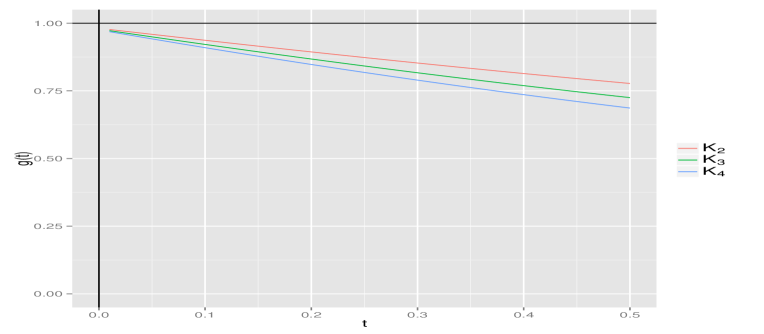
Figure 3.2. Plotting the function $g\left(t\right)$ over $t>0,$ for each kernel $K_{2},K_{3}$ and $K_{4}.$

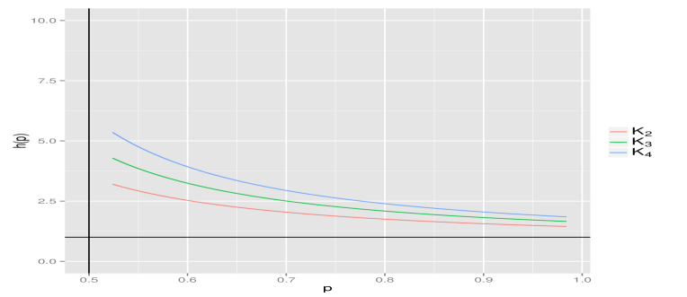
Figure 3.3. Plotting the function $h\left(p\right)$ over $\left(1/2,1\right),$ for each kernel $K_{2},K_{3}$ and $K_{4}.$

3.2. The optimal number of upper extremes

For a given kernel $K,$ we seek the optimal number of upper extremes $k_{K}^{\ast}$ that minimizes the asymptotic MSE which equals $\sigma_{K}^{2}/k+\left(k/n\right)^{2\gamma\beta_{\ast}}m_{K}^{2}=:\mathcal{M}\left(k\right).$ Explicitly we have

$$\mathcal{M}\left(k\right)\begin{tabular}[c]{l}$:=$\end{tabular}\ \frac{\gamma_{1}^{2}}{k}\int_{0}^{1}s^{-1/p+1}K^{2}\left(s\right)ds$$

$$\ \ \ \ \ \ \ \ \ \ \ \ \ \ \ \ \ +\mathbf{1}\left\{\beta_{1}\leq\beta_{2}\right\}\left(k/n\right)^{2\gamma\beta_{1}}\beta_{1}^{2}D_{1}^{2}C^{-2\gamma\beta_{1}}\gamma_{1}^{4}\left\{\int_{0}^{1}s^{\beta_{1}\gamma_{1}}K\left(s\right)ds\right\}^{2}.$$

Letting $\alpha:=\beta_{1}\gamma$ and $\mathcal{D}:=\mathbf{1}\left\{\beta_{1}\leq\beta_{2}\right\}D_{1}C^{-\alpha}p^{-1},$ we write

$$\gamma_{1}^{-2}\mathcal{M}\left(k\right)=\frac{1}{k}\int_{0}^{1}s^{-1/p+1}K^{2}\left(s\right)ds+\left(\frac{k}{n}\right)^{2\alpha}\left(\alpha\mathcal{D}\right)^{2}\left\{\int_{0}^{1}s^{\alpha/p}K\left(s\right)ds\right\}^{2}.$$

Using similar arguments as used to the proof of Theorem 5 in Csörgő et al. (1985), we infer that $k_{K}^{\ast}$ minimizing the right-side of the previous equation is the integer part of $n^{2\alpha/\left(2\alpha+1\right)}\left\{2\alpha^{3}\mathcal{D}^{3}\right\}^{-1/\left(2\alpha+1\right)}\Phi\left(K\right),$ where

$$\Phi\left(K\right):=\left\{\int_{0}^{1}s^{-1/p+1}K^{2}\left(s\right)ds\right\}^{1/\left(2\alpha+1\right)}\left\{\int_{0}^{1}s^{\alpha/p}K\left(s\right)ds\right\}^{-2/\left(2\alpha+1\right)}.$$

In particular, for the indicator kernel function $K_{1}:=\mathbf{1}\left\{\left[0,1\right)\right\},$ we have

$$\Phi\left(K_{1}\right) =\left\{\int_{0}^{1}s^{-1/p+1}ds\right\}^{1/\left(2\alpha+1\right)}\left\{\int_{0}^{1}s^{\alpha/p}ds\right\}^{-2/\left(2\alpha+1\right)}$$

$$=\left(\frac{p}{2p-1}\right)^{1/\left(2\alpha+1\right)}\left(\alpha/p+1\right)^{2/\left(2\alpha+1\right)}.$$

Thereby the optimal top $k$ observations used in Worms’s estimator $\widehat{\gamma}_{1,k}^{\left(W\right)}$ is

$$k_{W}^{\ast}=\left[n^{2/\left(2\alpha+1\right)}\left(\frac{2p\alpha^{3}\mathcal{D}^{3}}{2p-1}\right)^{1/\left(2\alpha+1\right)}\left(\alpha/p+1\right)^{2/\left(2\alpha+1\right)}\right].$$ (3.26)

Thus the ratio between the two optimal number of extremes is

$$\frac{k_{K}^{\ast}}{k_{W}^{\ast}}\sim\frac{\left\{\int_{0}^{1}s^{-1/p+1}K^{2}\left(s\right)ds\right\}^{1/\left(2\alpha+1\right)}\left\{\int_{0}^{1}s^{\alpha/p}K\left(s\right)ds\right\}^{-2/\left(2\alpha+1\right)}}{\left(\frac{p}{2p-1}\right)^{1/\left(2\alpha+1\right)}\left(\alpha/p+1\right)^{2/\left(2\alpha+1\right)}}.$$ (3.27)

Unfortunately, the optimal choice of the number of upper order statistics to be used in estimation depends mainly on the unknown slowly varying part of the tail. This fact makes obtaining a practical strategy for minimizing the asymptotic mean square error through an appropriate choice of $k$ difficult. There are numerous heuristic methods to select the optimal number of upper extremes used in the computation of the tail index estimate. An exhaustive bibliography to this topic is gathered in the nice survey given by Caeiro and Gomes (2015). Our choice fell on the method of Reiss and Thomas given in Reiss and Thomas (2007), page $137.$ In this procedure one defines the optimal sample fraction

$$k^{\ast}:=\arg\min_{1<k<n}\frac{1}{k}\sum_{i=1}^{k}i^{\nu}\left|\widehat{\gamma}_{1,i}-\text{median}\left\{\widehat{\gamma}_{1,1},...,\widehat{\gamma}_{1,k}\right\}\right|,$$

with suitable constant $0\leq\nu\leq 1/2,$ where $\widehat{\gamma}_{1,i}$ corresponds to the kernel estimator of tail index $\gamma_{1},$ based on the $i$ upper order statistics, of a Pareto-type model. We claim, in our simulation study below, that $\nu=0.3$ provides better results both in terms of bias and MSE. This agrees with that was found by Neves and Fraga Alves (2004) when considering Hill’s estimator in the non-truncation case. We will use this  procedure to select $k^{\ast}$ the optimal numbers of upper order statistics used in the computation of the all aforementioned estimators.

4. Simulation study

In this section we will perform a simulation study in order to compare the finite sample behavior of the kernel estimator $\widehat{\gamma}_{1,k},$ given in $\left(\ref{gtild}\right),$ with the three estimators $\widehat{\gamma}_{1,k}^{\left(EFG\right)},$ $\widehat{\gamma}_{1,k}^{\left(W\right)}$ and $\widehat{\gamma}_{1,k}^{\left(BAB\right)}\left(\mathcal{K}\right)$ stated respectively in $\left(\ref{AH}\right),$ $\left(\ref{WW}\right)$ and $\left(\ref{BAB}\right).$ We constructed the two estimator $\widehat{\gamma}_{1,k}$ and $\widehat{\gamma}_{1,k}^{\left(BAB\right)}\left(\mathcal{K}\right)$ by selecting the triweight kernel function $K_{3}$ (defined in $\left(\ref{Kfun}\right)),$ and $\mathcal{K}_{2}$ (given in in $\left(\ref{Kbis}\right))$ respectively. For the censoring and censored distributions functions $F$ and $G,$ will be chosen among the following two models:

• Burr $\left(\zeta,\gamma\right)$ distribution with right-tail function:

  $$\overline{\mathcal{L}}\left(x\right)=\left(1+x^{1/\zeta}\right)^{-\zeta/\gamma},\text{ }x\geq 0,\text{ }\zeta>0,\text{ }\gamma>0.$$

• Fréchet $\left(\gamma\right)$ distribution with right-tail function:

  $$\overline{\mathcal{L}}\left(x\right)=1-\exp\left(-x^{-1/\gamma}\right),\text{ }x>0,\text{ }\gamma>0.$$

For each given distribution, we generate $2000$ random samples of length $n$ $=$ $500$ and plot the four estimators, their corresponding biases and MSE’s as function of $k=1,...,500.$ We consider four scenarios, namely: a Burr distribution censored by another Burr distribution (Figure 4.4) a Fréchet distribution censored by another Fréchet distribution (Figure 4.5), a Burr distribution censored by a Fréchet distribution (Figure 4.6) and a Fréchet distribution censored by a Burr distribution (Figure 4.7). In each scenario, we considered the two censoring schemes, that is the weak censoring $\left(p>1/2\right)$ and the strong censoring $\left(p<1/2\right).$ The parametrization of Fréchet and Burr models is made so that it covers both the two situations $p>1/2$ and $p<1/2.$ In right panels of the four Figures 4.4-$\ref{Figure7},$ the simulation study shows that both kernel estimators $\widehat{\gamma}_{1,k}$ and $\widehat{\gamma}_{1,k}^{\left(BAB\right)}$ present a smoothness contrary to both estimators $\widehat{\gamma}_{1,k}^{\left(W\right)}$ and $\widehat{\gamma}_{1,k}^{\left(EFG\right)},$ which behave erratically a long the range of the largest extreme values $k.$ In addition, the two kernel estimators exhibit a stability and alignment with respect to the true value of the tail index $\gamma_{1}$ over almost the interval. We also point out that, in terms of stability, $\widehat{\gamma}_{1,k}$ performs better than $\widehat{\gamma}_{1,k}^{\left(BAB\right)}$ in the strong censoring case. We notice that $\widehat{\gamma}_{1,k}^{\left(W\right)}$ meets the true value of the tail index in a single point $k^{\ast}\in\left\{1,...,500\right\}$ while $\widehat{\gamma}_{1,k}^{\left(EFG\right)}$ does not cross the line $\gamma_{1}$ at any point, but approaches slightly this one on a small interval of $k.$ From the middle panels (resp. the right panels), in overall, $\widehat{\gamma}_{1,k}$ performs better than the three other estimators in terms of bias (resp. MSE) for the strong censoring case $\left(p>1/2\right),$ however $\widehat{\gamma}_{1,k}^{\left(W\right)}$ seems to be slightly better than $\widehat{\gamma}_{1,k}$ for the weak censoring $\left(p<1/2\right)$ one.

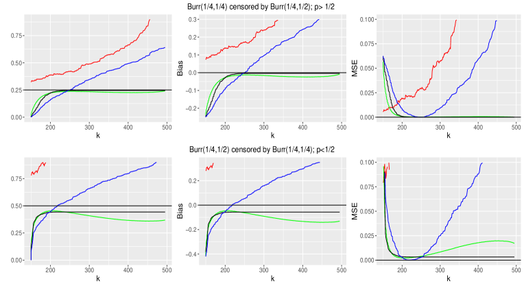
Figure 4.4. Comparison of the estimators (left-panels) $\widehat{\gamma}_{1,k}^{(EFG)}\left(\text{red line}\right),$ $\widehat{\gamma}_{1,k}^{(W)}\left(\text{blue line}\right),$ $\widehat{\gamma}_{1,k}^{(BAB)}\left(\text{green line}\right),$ $\widehat{\gamma}_{1,k}$ $\left(\text{black line}\right)$ their biases (middel-panels) and MSE’s (right-panels) for a Burr distribution censored by another Burr distribution with $p=2/3$ (top-panels) and $p=1/3$ (bottom-panels)

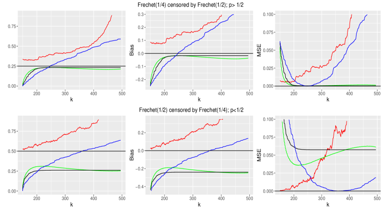
Figure 4.5. Comparison of the estimators (left-panels) $\widehat{\gamma}_{1,k}^{(EFG)}\left(\text{red line}\right),$ $\widehat{\gamma}_{1,k}^{(W)}\left(\text{blue line}\right),$ $\widehat{\gamma}_{1,k}^{(BAB)}\left(\text{green line}\right),$ $\widehat{\gamma}_{1,k}$ $\left(\text{black line}\right)$ their biases (middel-panels) and MSE’s (right-panels) for a Fréchet distribution censored by another Fréchet distribution with $p=2/3$ (top-panels) and $p=1/3$ (bottom-panels)

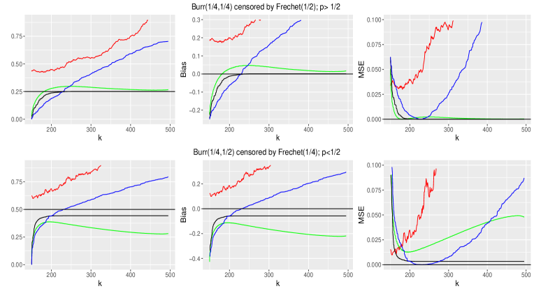
Figure 4.6. Comparison of the estimators (left-panels) $\widehat{\gamma}_{1,k}^{(EFG)}\left(\text{red line}\right),$ $\widehat{\gamma}_{1,k}^{(W)}\left(\text{blue line}\right),$ $\widehat{\gamma}_{1,k}^{(BAB)}\left(\text{green line}\right),$ $\widehat{\gamma}_{1,k}$ $\left(\text{black line}\right)$ their biases (middel-panels) and MSE’s (right-panels) for a Burr distribution censored by Fréchet distribution with $p=2/3$ (top-panels) and $p=1/3$ (bottom-panels)

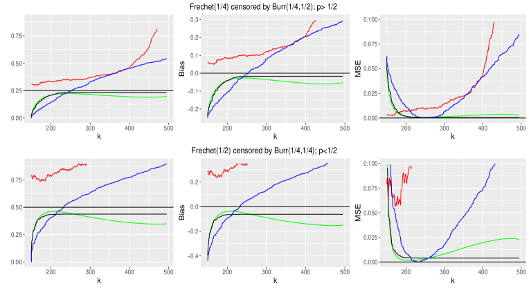
Figure 4.7. Comparison of the estimators (left-panels) $\widehat{\gamma}_{1,k}^{(EFG)}\left(\text{red line}\right),$ $\widehat{\gamma}_{1,k}^{(W)}\left(\text{blue line}\right),$ $\widehat{\gamma}_{1,k}^{(BAB)}\left(\text{green line}\right),$ $\widehat{\gamma}_{1,k}$ $\left(\text{black line}\right)$ their biases (middel-panels) and MSE’s (right-panels) for a Fréchet distribution censored by Burr distribution with $p=2/3$ (top-panels) and $p=1/3$ (bottom-panels)

5. Proofs

5.1. Proof of Theorem 3.1

We will adapt the proof of Theorem 1 in Beirlant et al. (2019) to the framework of the kernel estimation. To begin, let us define the following quantities

$$\widehat{RF}_{j}:=\frac{\overline{F}_{n}^{KM}\left(Z_{n-j+1:n}\right)}{\overline{F}_{n}^{KM}\left(Z_{n-k:n}\right)},\text{ }RF_{j}:=\frac{\overline{F}\left(Z_{n-j+1:n}\right)}{\overline{F}\left(Z_{n-k:n}\right)},$$

$$\widehat{RF}_{j}\left(K\right):=\frac{\overline{F}_{n}^{KM}\left(Z_{n-j+1:n}\right)}{\overline{F}_{n}^{KM}\left(Z_{n-k:n}\right)}K\left(\frac{\overline{F}_{n}^{KM}\left(Z_{n-j+1:n}\right)}{\overline{F}_{n}^{KM}\left(Z_{n-k:n}\right)}\right),\text{ }$$

and

$$RF_{j}\left(K\right):=\frac{\overline{F}\left(Z_{n-j+1:n}\right)}{\overline{F}\left(Z_{n-k:n}\right)}K\left(\frac{\overline{F}\left(Z_{n-j+1:n}\right)}{\overline{F}\left(Z_{n-k:n}\right)}\right).$$

For further use, we set

$$\xi_{j}:=j\log\frac{Z_{n-j+1:n}}{Z_{n-j:n}}\text{ and }E_{j}^{\left(n\right)}:=j\log\frac{Y_{n-j+1:n}}{Y_{n-j:n}},\text{ for }j=1,...,k,$$

where $Y_{1:n}\leq...\leq Y_{n:n}$ be the order statistics pertaining to the sample $\left(Y_{j}\right)_{1\leq j\leq n}$ of iid standard Pareto rv’s defined by $Z_{j}=U_{H}\left(Y_{j}\right),$ with

$$U_{H}\left(s\right):=\inf\left\{x,\text{ }H\left(x\right)\geq 1-1/s\right\},\text{ }s>1,$$ (5.28)

stands for the quantile function pertaining to cdf $H.$ Thanks to $\left(\ref{H}\right),$ we have

$$U_{H}\left(s\right)=C^{\gamma}s^{\gamma}\left(1+\gamma D_{\ast}C^{-\beta_{\ast}\gamma}s^{-\beta_{\ast}\gamma}\left(1+o\left(1\right)\right)\right),\text{ as }s\rightarrow\infty.$$ (5.29)

Since $\left\{\log Y_{j}\right\}_{1\leq j\leq k}$ are iid standard exponential rv’s, then the normalized spacings $\left\{E_{j}^{\left(n\right)}\right\}_{1\leq j\leq k}$ are iid standard exponential rv’s too; see for instance Theorem 4.6.1 in Arnold et al. (2008). The following approximation, given by Beirlant et al. (2002), will be one of the basic keys of the proof:

$$\xi_{j}=\xi_{j}^{\prime}+R_{j,n}\text{ where }\xi_{j}^{\prime}:=\left(\gamma+u_{j,k}^{\gamma\beta_{\ast}}b_{n,k}\right)E_{j}^{\left(n\right)},$$ (5.30)

with $u_{j,k}:=\frac{j}{k+1}$ and $b_{n,k}=-\left(1+o_{\mathbf{P}}\left(1\right)\right)\gamma^{2}\beta_{\ast}D_{\ast}C^{-\gamma\beta_{\ast}}\left(\frac{k+1}{n+1}\right)^{\gamma\beta_{\ast}},$ as $n\rightarrow\infty.$ The remainder term $R_{j,n}$ is described in Theorem 2.1 of the aforementioned paper, which satisfies $\left|\sum_{i=j}^{k}i^{-1}R_{i,n}\right|=o_{\mathbf{P}}\left(b_{n,k}\log\left(\max\left(u_{j,k}^{-1},1\right)\right)\right).$ Next we show that, in the same probability space $\left(\Omega,\mathcal{A},\mathbf{P}\right),$ there exists a sequence of iid standard uniform rv’s $\left(U_{i}\right)_{1\leq i\leq k}$ independent to $\left(E_{i}^{\left(n\right)}\right)_{1\leq i\leq k},$ such that

$$\sqrt{k}\left(\widehat{\gamma}_{1,k}-\gamma_{1}\right)-m_{K}\left\{\sqrt{k}\left(k/n\right)^{\gamma\beta_{\ast}}\right\}$$

$$=\gamma\frac{\sqrt{k}}{k+1}\sum_{i=2}^{k}\left\{u_{i,k}^{-1}\sum_{j=2}^{i}u_{j,k}^{p-1}g_{K}^{\prime}\left(u_{j,k}^{p}\right)\right\}\mathcal{A}_{i,n}+o_{\mathbf{P}}\left(1\right),$$ (5.31)

where $g_{K}\left(s\right)=sK\left(s\right),$ $\mathcal{A}_{i,n}:=p\left(E_{i}^{\left(n\right)}-1\right)-\left(\mathbf{1}\left\{U_{i}\leq p\right\}-p\right)$ and $m_{K}$ is as in $\left(\ref{mk}\right).$ To this end, let us rewrite formula $\left(\ref{KF}\right)$ into

$$\widehat{\gamma}_{1,k}=\sum_{j=2}^{k}\frac{\overline{F}_{n}^{KM}\left(Z_{n-j+1:n}\right)}{\overline{F}_{n}^{KM}\left(Z_{n-k:n}\right)}K\left(\frac{\overline{F}_{n}^{KM}\left(Z_{n-j+1:n}\right)}{\overline{F}_{n}^{KM}\left(Z_{n-k:n}\right)}\right)\left\{\log\frac{Z_{n-j+1:n}}{Z_{n-k:n}}-\log\frac{Z_{n-j:n}}{Z_{n-k:n}}\right\}.$$

It is easy to verify that $\widehat{\gamma}_{1,k}-\gamma_{1}$ may be decomposed into the sum of

$$T_{k,n}^{\left(1\right)}:=\sum_{j=2}^{k}\left(\widehat{RF}_{j}\left(K\right)-RF_{j}\left(K\right)\right)\frac{\xi_{j}^{\prime}}{j},\text{ }T_{k,n}^{\left(2\right)}:=\sum_{j=2}^{k}RF_{j}\left(K\right)\frac{\xi_{j}^{\prime}}{j}-\frac{\gamma}{k+1}\sum_{j=2}^{k}K\left(u_{j,k}^{p}\right),$$

$$T_{k,n}^{\left(3\right)}:=\frac{\gamma}{k+1}\sum_{j=2}^{k}K\left(u_{j,k}^{p}\right)-\gamma_{1}\text{ and }T_{k,n}^{\left(4\right)}:=\sum_{j=2}^{k}\widehat{RF}_{j}\left(K\right)\frac{R_{j,n}}{j}.$$

It is worth mentioning that, by considering the indicator kernel function $K_{1},$ the last three (remainder) terms $T_{k,n}^{\left(i\right)},$ $i=2,3,4$ coincide with those stated in the beginning of the proof of Theorem 1 in Beirlant et al. (2019). The authors showed that these terms, times $\sqrt{k},$ tend to zero in probability as $n\rightarrow\infty.$ By deep reading the proof, we came to the conclusion that by using the assumption $\left[A4\right]$ on kernel $K$ we end up with $\sqrt{k}T_{k,n}^{\left(i\right)}=o_{\mathbf{P}}\left(1\right),$ $i=2,3,4$ as $n\rightarrow\infty,$ as well, that we omit details. This means that $T_{k,n}^{\left(1\right)}$ is the only term that contributes to the asymptotic normality of $\widehat{\gamma}_{1,k}.$ Indeed, using Taylor’s expansion of second-order to this one yields

$$T_{k,n}^{\left(1\right)} =\sum_{j=2}^{k}\left(\widehat{RF}_{j}-RF_{j}\right)g_{K}^{\prime}\left(RF_{j}\right)\frac{\xi_{j}^{\prime}}{j}+\frac{1}{2}\sum_{j=2}^{k}\left(\widehat{RF}_{j}-RF_{j}\right)^{2}g_{K}^{\prime\prime}\left(\widetilde{RF}_{j}\right)\frac{\xi_{j}^{\prime}}{j}$$

$$=\mathcal{T}_{k,n}^{\left(1\right)}+\mathcal{R}_{k,n}^{\left(1\right)},$$

where $\widetilde{RF}_{j}$ is a rv between $\widehat{RF}_{j}$ and $RF_{j}.$ From assumption $\left[A4\right],$ the function $g_{K}^{\prime\prime}$ is bounded, then using similar arguments of the proof in A.3.2 given in Beirlant et al. (2019), we show that $\sqrt{k}\mathcal{R}_{k,n}^{\left(1\right)}=o_{\mathbf{P}}\left(1\right),$ as $n\rightarrow\infty.$ Let us now focus on the term $\mathcal{T}_{k,n}^{\left(1\right)}$ which may be made into the sum of

$$\mathcal{T}_{k,n}^{\left(1,1\right)}:=\sum_{j=2}^{k}\left\{\log\frac{\widehat{RF}_{j}}{RF_{j}}\right\}RF_{j}g_{K}^{\prime}\left(RF_{j}\right)\frac{\xi_{j}^{\prime}}{j}$$

and

$$\mathcal{T}_{k,n}^{\left(1,2\right)}:=\sum_{j=2}^{k}\left\{-\log\frac{\widehat{RF}_{j}}{RF_{j}}+\left(\frac{\widehat{RF}_{j}}{RF_{j}}-1\right)\right\}RF_{j}g_{K}^{\prime}\left(RF_{j}\right)\frac{\xi_{j}^{\prime}}{j}.$$

It easy to check that $\log\widehat{RF}_{j}=\sum_{i=j}^{k}\delta_{\left(n-i+1\right)}\log\frac{i-1}{i},$ therefore

$$\mathcal{T}_{k,n}^{\left(1,1\right)}=\sum_{j=2}^{k}\left(\sum_{i=j}^{k}\delta_{\left(n-i+1\right)}\log\frac{i-1}{i}-\log RF_{j}\right)RF_{j}g_{K}^{\prime}\left(RF_{j}\right)\frac{\xi_{j}^{\prime}}{j}.$$

Note that $\sum_{i=j}^{k}\xi_{i}/i=\log\left(Z_{n-j+1:n}/Z_{n-k:n}\right)$ and

$$\log RF_{j}=\frac{-1}{\gamma_{1}}\sum_{i=j}^{k}\frac{\xi_{i}}{i}+\left(\log RF_{j}+\frac{1}{\gamma_{1}}\log\frac{Z_{n-j+1:n}}{Z_{n-k:n}}\right),$$

it follows that

$$\mathcal{T}_{k,n}^{\left(1,1\right)} =\sum_{j=2}^{k}\left(\frac{1}{\gamma_{1}}\sum_{i=j}^{k}\frac{\xi_{i}}{i}+\sum_{i=j}^{k}\delta_{\left(n-i+1\right)}\log\frac{i-1}{i}\right)RF_{j}g_{K}^{\prime}\left(RF_{j}\right)\frac{\xi_{j}^{\prime}}{j}$$

$$\ \ \ -\sum_{j=2}^{k}\left\{\log RF_{j}+\frac{1}{\gamma_{1}}\log\frac{Z_{n-j+1:n}}{Z_{n-k:n}}\right\}RF_{j}g_{K}^{\prime}\left(RF_{j}\right)\frac{\xi_{j}^{\prime}}{j}.$$

Observe that the first term equals

$$\sum_{j=2}^{k}\sum_{i=j}^{k}\left(\frac{1}{\gamma_{1}}\frac{\xi_{i}}{i}+\delta_{\left(n-i+1\right)}\log\frac{i-1}{i}\right)RF_{j}g_{K}^{\prime}\left(RF_{j}\right)\frac{\xi_{j}^{\prime}}{j},$$

which, by inverting the sums, becomes $\sum_{i=2}^{k}\left(\frac{1}{\gamma_{1}}\xi_{i}+\delta_{\left(n-i+1\right)}i\log\frac{i-1}{i}\right)S_{i,k},$  where $S_{i,k}:=\frac{1}{i}\sum_{j=2}^{i}RF_{j}g_{K}^{\prime}\left(RF_{j}\right)\frac{\xi_{j}^{\prime}}{j},$ $j=2,...,k.$ Thereby $\mathcal{T}_{k,n}^{\left(1,1\right)}$ may be rewritten into

$$\begin{array}[c]{cc}{\displaystyle\sum\limits_{i=2}^{k}}\left(\dfrac{1}{\gamma_{1}}\left(\xi_{i}-\gamma\right)+\delta_{\left(n-i+1\right)}i\log\dfrac{i-1}{i}+p\right)S_{i,k}\vskip 6.0pt plus 2.0pt minus 2.0pt&\\ -{\displaystyle\sum\limits_{j=2}^{k}}\left(\log RF_{j}+\dfrac{1}{\gamma_{1}}\log\dfrac{Z_{n-j+1:n}}{Z_{n-k:n}}\right)RF_{j}g_{K}^{\prime}\left(RF_{j}\right)\dfrac{\xi_{j}^{\prime}}{j}&=\mathcal{T}_{k,n}^{\left(1,1,1\right)}-\mathcal{T}_{k,n}^{\left(1,1,2\right)}.\end{array}$$

We need to the following additional notations:

$$c_{i}:=1+i\log\frac{i-1}{i},\text{ }A_{i,n}:=p\left(E_{i}^{\left(n\right)}-1\right)-\left(\delta_{\left(n-i+1\right)}-p\right)\text{ and }B_{i,n}:=\frac{1}{\gamma_{1}}b_{n,k}u_{i,k}^{\beta_{\ast}\gamma}E_{i}^{\left(n\right)}.$$

By adding $\delta_{\left(n-i+1\right)}$ and subtracting it, then by using the approximation $\left(\ref{ksiprime}\right),$ we rewrite $\mathcal{T}_{k,n}^{\left(1,1,1\right)}$ into

$$\mathcal{T}_{k,n}^{\left(1,1,1\right)}=\sum_{i=2}^{k}A_{i,n}S_{i,k}+\sum_{i=2}^{k}B_{i,n}S_{i,k}+\sum_{i=2}^{k}\delta_{\left(n-i+1\right)}c_{i}S_{i,k}+\gamma_{1}^{-1}\sum_{i=2}^{k}R_{i,n}S_{i,k}.$$

Once again, using assumption $\left[A4\right]$ and Proposition (parts c and d) in Beirlant et al. (2019), we infer that $\sqrt{k}\sum_{i=2}^{k}\delta_{\left(n-i+1\right)}c_{i}S_{i,k}=o_{\mathbf{P}}\left(1\right)=\sqrt{k}\sum_{i=2}^{k}R_{i,n}S_{i,k},$ as $n\rightarrow\infty.$ Next we show that

$$\sqrt{k}\sum_{i=2}^{k}A_{i,n}S_{i,k}=\mathcal{N}\left(0,\gamma_{1}^{2}\int_{0}^{1}t^{-1/p+1}K^{2}\left(t\right)dt\right)+\mathcal{B}_{1,k}+o_{\mathbf{p}}\left(1\right),$$ (5.32)

and $\sqrt{k}\sum_{i=2}^{k}B_{i,n}S_{i,k}=\mathcal{B}_{2,k}+o_{\mathbf{P}}\left(1\right),$ where $\mathcal{B}_{1,k}$ and $\mathcal{B}_{2,k}$ are asymptotic two biases that we precise later on. Indeed, let us decompose $\sum_{i=2}^{k}A_{i,n}S_{i,k}$ into the sum of

$$\mathcal{I}_{n1}:=\sum_{i=2}^{k}A_{i,n}\left\{\frac{1}{i}\sum_{j=2}^{i}u_{j,k}^{p}g_{K}^{\prime}\left(u_{j,k}^{p}\right)\frac{\xi_{j}^{\prime}}{j}\right\},$$

$$\mathcal{I}_{n2}:=\sum_{i=2}^{k}A_{i,n}\left\{\frac{1}{i}\sum_{j=2}^{i}\left\{V_{j,k}^{p}g_{K}^{\prime}\left(V_{j,k}^{p}\right)-u_{j,k}^{p}g_{K}^{\prime}\left(u_{j,k}^{p}\right)\right\}\frac{\xi_{j}^{\prime}}{j}\right\}$$

and

$$\mathcal{I}_{n3}:=\sum_{i=2}^{k}A_{i,n}\left\{\frac{1}{i}\sum_{j=2}^{i}V_{j,k}^{p}g_{K}^{\prime}\left(V_{j,k}^{p}\right)C_{j,k,0}\frac{\xi_{j}^{\prime}}{j}\right\},$$

where $C_{j,k,0}$ is a sequence of constants defined in assertion $\left(33\right)$ in Beirlant et al. (2019). By means of Taylor’s expansion to function $t\rightarrow tg_{K}^{\prime}\left(t\right),$ with assumption $\left[A4\right],$ and similar arguments as used to terms $I_{n2}$ and $I_{n3}$ in Beirlant et al. (2019), we infer that $\sqrt{k}\mathcal{I}_{n2}=o_{\mathbf{P}}\left(1\right)=\sqrt{k}\mathcal{I}_{n3}.$ Recall, from representation $\left(\ref{ksiprime}\right),$ that $\xi_{j}^{\prime}$ may be rewritten into $\gamma+\gamma\left(E_{j}^{\left(n\right)}-1\right)+b_{n,k}u_{j,k}^{\gamma\beta_{\ast}}E_{j}^{\left(n\right)},$ this allows us to decompose the first term $\mathcal{I}_{n1}$ into the sum of

$$\mathcal{I}_{n1}^{\left(1\right)}:=\gamma\sum_{i=2}^{k}A_{i,n}\left\{\frac{1}{i}\sum_{j=2}^{i}u_{j,k}^{p}g_{K}^{\prime}\left(u_{j,k}^{p}\right)\frac{1}{j}\right\}.$$

$$\mathcal{I}_{n1}^{\left(2\right)}:=\gamma\sum_{i=2}^{k}A_{i,n}\left\{\frac{1}{i}\sum_{j=2}^{i}u_{j,k}^{p}g_{K}^{\prime}\left(u_{j,k}^{p}\right)\frac{E_{j}^{\left(n\right)}-1}{j}\right\}$$

and

$$\mathcal{I}_{n1}^{\left(3\right)}:=b_{n,k}\sum_{i=2}^{k}A_{i,n}\left\{\frac{1}{i}\sum_{j=2}^{i}u_{j,k}^{p}g_{K}^{\prime}\left(u_{j,k}^{p}\right)\frac{u_{j,k}^{\gamma\beta_{\ast}}}{j}E_{j}^{\left(n\right)}\right\}.$$

Since $g_{K}^{\prime}$ is bounded, then using similar arguments as used to the terms $I_{1,n}^{\left(2\right)}$ and $I_{1,n}^{\left(3\right)}$ in Beirlant et al. (2019), we show that $\sqrt{k}\mathcal{I}_{n1}^{\left(2\right)}=o_{\mathbf{P}}\left(1\right)=\sqrt{k}\mathcal{I}_{n1}^{\left(3\right)}$ as well, that we omit the details. Let us now focus on the first term

$$\mathcal{I}_{n1}^{\left(1\right)}=\frac{\gamma}{k+1}\sum_{i=2}^{k}\left\{\frac{1}{i}\sum_{j=2}^{i}u_{j,k}^{p-1}g_{K}^{\prime}\left(u_{j,k}^{p}\right)\right\}\left\{p\left(E_{i}^{\left(n\right)}-1\right)-\left(\delta_{\left(n-i+1\right)}-p\right)\right\}.$$

Einmahl et al. (2008) showed that the sequence of rv’s $\delta_{\left(i\right)}$ may be approximated by iid Bernoulli rv’s $\mathbf{1}\left\{U_{i}\leq p\right\},$ where $U_{i}$ is a sequence of standard uniform rv’s which are independent to $E_{i}^{\left(n\right)}.$ Moreover the authors claim that

$$\delta_{\left(i\right)}=\mathbf{1}\left\{U_{i}\leq p\left(Z_{i:n}\right)\right\}=\mathbf{1}\left\{U_{i}\leq p\circ U_{H}\left(Y_{i:n}\right)\right\},$$

where $p\left(\cdot\right)$ is the function defined in Section $\ref{sec2}.$ In order to use this approximation, let us decompose $\mathcal{I}_{n1}^{\left(1\right)}$ into the sum of

$$\mathcal{L}_{n1}^{\left(1\right)}:=\gamma\frac{\sqrt{k}}{k+1}\sum_{i=2}^{k}\left\{\frac{1}{i}\sum_{j=2}^{i}u_{j,k}^{p-1}g_{K}^{\prime}\left(u_{j,k}^{p}\right)\right\}\left(p\left(E_{i}^{\left(n\right)}-1\right)-\left(\mathbf{1}\left\{U_{n-i+1}\leq p\right\}-p\right)\right),$$

$$\mathcal{L}_{n1}^{\left(2\right)}\begin{array}[c]{c}:=\end{array}-\gamma\frac{\sqrt{k}}{k+1}\sum_{i=2}^{k}\left\{\frac{1}{i}\sum_{j=2}^{i}u_{j,k}^{p-1}g_{K}^{\prime}\left(u_{j,k}^{p}\right)\right\}$$

$$\ \ \ \ \ \ \ \ \ \ \ \ \ \ \ \ \ \times\left(\mathbf{1}\left\{U_{n-i+1}\leq p\circ U_{H}\left(n/i\right)\right\}-\mathbf{1}\left\{U_{n-i+1}\leq p\right\}\right)$$

and

$$\mathcal{L}_{n1}^{\left(3\right)}\begin{array}[c]{c}:=\end{array}\gamma\frac{\sqrt{k}}{k+1}\sum_{i=2}^{k}\left\{\frac{1}{i}\sum_{j=2}^{i}u_{j,k}^{p-1}g_{K}^{\prime}\left(u_{j,k}^{p}\right)\right\}$$

$$\ \ \ \ \ \ \ \ \ \ \ \ \ \ \times\left(\mathbf{1}\left\{U_{n-i+1}\leq p\circ U_{H}\left(n/i\right)\right\}-\mathbf{1}\left\{U_{n-i+1}\leq p\circ U_{H}\left(Y_{n-i+1:n}\right)\right\}\right).$$

Note that the symbol $f_{1}\circ f_{2}$ sands for the composition of two functions $f_{1}$ and $f_{2}.$ Note that $\left(U_{n-i+1}\right)_{1\leq i\leq n}\overset{\mathcal{D}}{=}\left(U_{i}\right)_{1\leq i\leq n}$ and $\left(E_{i}^{\left(n\right)}\right)_{1\leq i\leq k}\overset{\mathcal{D}}{=}\left(E_{i}\right)_{1\leq i\leq k},$ where $\left(E_{i}^{\left(n\right)}\right)_{1\leq i\leq k}$ is a sequence of iid standard exponential rv’s, then without loss of generality we may write

$$\mathcal{L}_{n1}^{\left(1\right)}=\gamma\frac{\sqrt{k}}{k+1}\sum_{i=2}^{k}\left\{\frac{1}{i}\sum_{j=2}^{i}u_{j,k}^{p-1}g_{K}^{\prime}\left(u_{j,k}^{p}\right)\right\}\left(p\left(E_{i}-1\right)-\left(\mathbf{1}\left\{U_{i}\leq p\right\}-p\right)\right).$$

Observe that this last may be decomposed into the sum of

$$\mathcal{L}_{n1}^{\left(1,1\right)}:=\gamma\frac{\sqrt{k}}{k+1}\sum_{i=2}^{k}d_{i,k}\left(g_{K}\right)\left(p\left(E_{i}-1\right)-\left(\mathbf{1}\left\{U_{i}\leq p\right\}-p\right)\right),$$

and

$$\mathcal{L}_{n1}^{\left(1,2\right)}:=\gamma\frac{\sqrt{k}}{k+1}\sum_{i=2}^{k}\left\{u_{i,k}^{-1}\int_{0}^{u_{i,k}}s^{p-1}g_{K}^{\prime}\left(s^{p}\right)ds\right\}\left(p\left(E_{i}-1\right)-\left(\mathbf{1}\left\{U_{i}\leq p\right\}-p\right)\right),$$

where $d_{i,k}\left(g_{K}\right):=\frac{1}{i}\sum_{j=2}^{i}u_{j,k}^{p-1}g_{K}^{\prime}\left(u_{j,k}^{p}\right)-u_{i,k}^{-1}\int_{0}^{u_{i,k}}s^{p-1}g_{K}^{\prime}\left(s^{p}\right)ds.$ Making use of Lemma 6.1 (see the Appendix) and using similar arguments as used to the term $R_{k,n}$ in the proof of Proposition $1$ (part (a)) in Beirlant et al. (2019), we show that $\mathcal{L}_{n1}^{\left(1,1\right)}=o_{\mathbf{P}}\left(1\right),$ that we omit further details. It is clear that the variance of $p\left(E_{i}-1\right)-\left(\mathbf{1}\left\{U_{i}\leq p\right\}-p\right)$ equals $p^{2}+p\left(1-p\right)=p,$ thus using Lyapunov’s central limit theorem (for triangular arrays), we get

$$\mathcal{L}_{n1}^{\left(1,2\right)}\overset{\mathcal{D}}{\rightarrow}\mathcal{N}\left(0,p\gamma^{2}\int_{0}^{1}s^{-2}\left(\int_{0}^{s}t^{p-1}g_{K}^{\prime}\left(t^{p}\right)dt\right)^{2}ds\right),\text{ as }n\rightarrow\infty.$$

By using a change of variables, we readily showed that

$$p\gamma^{2}\int_{0}^{1}s^{-2}\left(\int_{0}^{s}t^{p-1}g_{K}^{\prime}\left(t^{p}\right)dt\right)^{2}ds=\gamma_{1}^{2}\int_{0}^{1}t^{-1/p+1}K^{2}\left(t\right)dt.$$

Let us consider the second term $\mathcal{L}_{n1}^{\left(2\right)}.$ From assertion $\left(57\right)$ in Beirlant et al. (2019), we infer that $p\circ U_{H}\left(n/i\right)-p=p\left(1-p\right)\left(D_{\gamma}\right)_{\ast}\beta_{\ast}C^{-\gamma\beta_{\ast}}\left(i/n\right)^{\gamma\beta_{\ast}}\left(1+o\left(1\right)\right),$ where

$$\left(D_{\gamma}\right)_{\ast}:=\gamma_{1}D_{1}\mathbf{1}\left\{\beta_{1}<\beta_{2}\right\}-\gamma_{2}D_{2}\mathbf{1}\left\{\beta_{1}>\beta_{2}\right\}+\left(\gamma_{1}D_{1}-\gamma_{2}D_{2}\right)\mathbf{1}\left\{\beta_{1}=\beta_{2}\right\}.$$

It follows that

$$\mathcal{L}_{n1}^{\left(2\right)}=-\gamma p\left(1-p\right)\left(D_{\gamma}\right)_{\ast}\beta_{\ast}C^{-\gamma\beta_{\ast}}\frac{\sqrt{k}}{k+1}\sum_{i=2}^{k}\left\{i^{-1}\sum_{j=2}^{i}u_{j,k}^{p-1}g_{K}^{\prime}\left(u_{j,k}^{p}\right)\right\}\left(i/n\right)^{\gamma\beta_{\ast}},$$

which may be decomposed into the sum of

$$\mathcal{L}_{n1}^{\left(2,1\right)}:=-\gamma p\left(1-p\right)\left(D_{\gamma}\right)_{\ast}\beta_{\ast}C^{-\gamma\beta_{\ast}}\frac{\sqrt{k}}{k+1}\sum_{i=2}^{k}\left\{u_{i,k}^{-1}\int_{0}^{u_{i,k}}s^{p-1}g_{K}^{\prime}\left(s^{p}\right)\right\}\left(i/n\right)^{\gamma\beta_{\ast}}$$

and

$$\mathcal{L}_{n1}^{\left(2,2\right)}:=-\gamma p\left(1-p\right)\left(D_{\gamma}\right)_{\ast}\beta_{\ast}C^{-\gamma\beta_{\ast}}\frac{\sqrt{k}}{k+1}\sum_{i=2}^{k}d_{i,k}\left(g_{K}\right)\left(i/n\right)^{\gamma\beta_{\ast}}.$$

Observe that $\mathcal{L}_{n1}^{\left(2,1\right)}=\left\{\frac{1}{k+1}\sum_{i=2}^{k}\left(u_{i,k}^{-1+\gamma\beta_{\ast}}\int_{0}^{u_{i,k}}s^{p-1}g_{K}^{\prime}\left(s^{p}\right)\right)\right\}b_{1,k},$ where $b_{1,k}:=-\gamma p\left(1-p\right)\left(D_{\gamma}\right)_{\ast}\beta_{\ast}C^{-\gamma\beta_{\ast}}\sqrt{k}\left(\frac{k+1}{n}\right)^{\gamma\beta_{\ast}}.$ The quantity between two braces is a Riemann sum, which converges, as $n\rightarrow\infty,$ to

$$\int_{0}^{1}s^{-1+\gamma\beta_{\ast}}\left(\int_{0}^{s}t^{p-1}g_{K}^{\prime}\left(t^{p}\right)dt\right)ds=\frac{1}{p^{2}}\int_{0}^{1}t^{\gamma_{1}\beta_{\ast}}K\left(t\right)dt.$$

Recall that $\sqrt{k}\left(\frac{k}{n}\right)^{\gamma\beta_{\ast}}=O_{\mathbf{P}}\left(1\right),$ then $\sqrt{k}\left(\frac{k+1}{n}\right)^{\gamma\beta_{\ast}}=\sqrt{k}\left(\frac{k}{n}\right)^{\gamma\beta_{\ast}}+o_{\mathbf{P}}\left(1\right),$ thus $\mathcal{L}_{n1}^{\left(2,1\right)}=\mathcal{B}_{1,k}+o_{\mathbf{P}}\left(1\right),$ where

$$\mathcal{B}_{1,k}:=-\gamma_{1}\left(1-p\right)\left(D_{\gamma}\right)_{\ast}\beta_{\ast}C^{-\gamma\beta_{\ast}}\int_{0}^{1}t^{\gamma_{1}\beta_{\ast}}K\left(t\right)dt\left\{\sqrt{k}\left(k/n\right)^{\gamma\beta_{\ast}}\right\}.$$ (5.33)

Once again, making use of Lemma $\ref{lemma1},$ we show that

$$\mathcal{L}_{n1}^{\left(2,2\right)}=O_{\mathbf{P}}\left(1\right)k^{-1/2+p}\left(k/n\right)^{\gamma\beta_{\ast}}\left\{k^{-1}\sum_{i=1}^{k}u_{i,k}^{-1+\gamma\beta_{\ast}}\right\},$$

as $n\rightarrow\infty.$ Since $k^{-1}\sum_{i=1}^{k}u_{i,k}^{-1+\gamma\beta_{\ast}}$ converges to $\int_{0}^{1}s^{-1+\gamma\beta_{\ast}}ds=1/\gamma\beta_{\ast}$ (Riemann sum) and both $k^{-1/2+p}$ and $\left(k/n\right)^{\gamma\beta_{\ast}}$ tend to zero, this means that $\mathcal{L}_{n1}^{\left(2,2\right)}=o_{\mathbf{P}}\left(1\right),$ thus $\mathcal{L}_{n1}^{\left(2\right)}=\mathcal{B}_{1,k}+o_{\mathbf{P}}\left(1\right).$ To finish with the term $\mathcal{L}_{n1},$ we will also show that $\sqrt{k}\mathcal{L}_{n1}^{\left(3\right)}=o_{\mathbf{P}}\left(1\right)$ as $n\rightarrow\infty.$ Recall that $g_{K}^{\prime}$ is a bounded, then

$$\mathcal{L}_{n1}^{\left(3\right)} =O_{\mathbf{P}}\left(1\right)\frac{\sqrt{k}}{k+1}\sum_{i=2}^{k}\left\{u_{i,k}^{-1}\sum_{j=2}^{i}u_{j,k}^{p-1}\right\}$$

$$\times\left|\mathbf{1}\left\{U_{n-i+1}\leq p\circ U_{H}\left(Y_{n-i+1:n}\right)\right\}-\mathbf{1}\left\{U_{n-i+1}\leq p\circ U_{H}\left(n/i\right)\right\}\right|.$$

By using similar arguments as used for the term $B_{1,k}^{\left(1\right)}$ in Beirlant et al. (2019), we show that $\sqrt{k}\mathcal{L}_{n1}^{\left(3\right)}=o_{\mathbf{P}}\left(1\right),$ therefore we omit details. We now consider the term

$$\sum_{i=2}^{k}B_{i,n}S_{i,k}=\frac{1}{\gamma_{1}}b_{n,k}\sum_{i=2}^{k}u_{i,k}^{\beta_{\ast}\gamma}\left(\frac{1}{i}\sum_{j=2}^{i}RF_{j}g_{K}^{\prime}\left(RF_{j}\right)\frac{\xi_{j}^{\prime}}{j}\right)E_{i}^{\left(n\right)}.$$

By using similar decomposition as used to the term $\sum_{i=2}^{k}A_{i,n}S_{i,k},$ we end up with

$$\sum_{i=2}^{k}B_{i,n}S_{i,k} =\left(1+o_{\mathbf{P}}\left(1\right)\right)\frac{1}{\gamma_{1}}b_{n,k}\frac{1}{k+1}\sum_{i=2}^{k}u_{i,k}^{\beta_{\ast}\gamma}\left(\frac{1}{i}\sum_{j=2}^{i}u_{j,k}^{p-1}g_{K}^{\prime}\left(u_{j,k}^{p}\right)\xi_{j}^{\prime}\right)E_{i}$$

$$=\left(1+o_{\mathbf{P}}\left(1\right)\right)pb_{n,k}\left\{\frac{1}{k+1}\sum_{i=2}^{k}u_{i,k}^{\beta_{\ast}\gamma}\left(\frac{1}{i}\sum_{j=2}^{i}u_{j,k}^{p-1}g_{K}^{\prime}\left(u_{j,k}^{p}\right)\right)E_{i}\right\}.$$

From Lemma 6.2 the previous factor between two braces converges in probability, as $n\rightarrow\infty,$ to $p^{-2}\int_{0}^{1}t^{\gamma_{1}\beta_{\ast}}K\left(t\right)dt,$ therefore $\sqrt{k}\sum_{i=2}^{k}B_{i,n}S_{i,k}=\mathcal{B}_{2,k}+o_{\mathbf{P}}\left(1\right),$ where

$$\mathcal{B}_{2,k}:=-\gamma^{2}\beta_{\ast}D_{\ast}C^{-\gamma\beta_{\ast}}p^{-1}\int_{0}^{1}t^{\gamma_{1}\beta_{\ast}}K\left(t\right)dt\left\{\sqrt{k}\left(k/n\right)^{\gamma\beta_{\ast}}\right\}.$$ (5.34)

In conclusion, we showed that $\sqrt{k}\mathcal{T}_{k,n}^{\left(1,1,1\right)}=\mathcal{N}\left(0,\sigma_{K}^{2}\right)+\mathcal{B}_{1,k}+\mathcal{B}_{2,k}+o_{\mathbf{P}}\left(1\right).$ Let us now consider the term $\mathcal{T}_{k,n}^{\left(1,1,2\right)}.$ Following the same steps as used in the proof of subsection A.3.3 in Beirlant et al. (2019), we show that $\sqrt{k}\mathcal{T}_{k,n}^{\left(1,1,2\right)}=\mathcal{B}_{3,k}+o_{\mathbf{P}}\left(1\right),$ where

$$\mathcal{B}_{3,k}:=-\gamma^{2}\beta_{\ast}D_{1}C^{-\gamma\beta_{\ast}}p^{-2}\int_{0}^{1}t^{\gamma_{1}\beta_{\ast}}K\left(t\right)dt\left\{\sqrt{k}\left(k/n\right)^{\gamma\beta_{\ast}}\right\}\mathbf{1}\left\{\beta_{1}\leq\beta_{2}\right\},$$ (5.35)

thereby $\sqrt{k}\mathcal{T}_{k,n}^{\left(1,1\right)}=\mathcal{N}\left(0,\sigma_{K}^{2}\right)+\mathcal{B}_{1,k}+\mathcal{B}_{2,k}-\mathcal{B}_{3,k}+o_{\mathbf{P}}\left(1\right).$ Using similar arguments as used to the proof given in subsection A.3.2 of the same paper, we also show that $\sqrt{k}\mathcal{T}_{k,n}^{\left(1,2\right)}=\mathcal{B}_{4,k}+o_{\mathbf{P}}\left(1\right),$ where

$$\mathcal{B}_{4,k}:=-\gamma^{2}\beta_{\ast}\left(D_{\ast}+\frac{D^{\ast}}{p}\right)C^{-\gamma\beta_{\ast}}p^{-1}\int_{0}^{1}t^{\gamma_{1}\beta_{\ast}}K\left(t\right)dt\left\{\sqrt{k}\left(\frac{k}{n}\right)^{\gamma\beta_{\ast}}\right\},$$ (5.36)

with $D^{\ast}:=-pD_{\ast}\mathbf{1}\left\{\beta_{2}<\beta_{1}\right\}+\left(D_{1}-pD_{\ast}\right)\mathbf{1}\left\{\beta_{1}\leq\beta_{2}\right\}.$ To summarize, we showed that

$$\sqrt{k}\left(\widehat{\gamma}_{1,k}-\gamma_{1}\right)=\mathcal{L}_{n1}^{\left(1,1\right)}+\mathcal{B}_{k}+o_{\mathbf{P}}\left(1\right),\text{ as }n\rightarrow\infty,$$ (5.37)

where $\mathcal{L}_{n1}^{\left(1,1\right)}\overset{D}{\rightarrow}\mathcal{N}\left(0,\sigma_{K}^{2}\right)$ and $\mathcal{B}_{k}:=\mathcal{B}_{1,k}+\mathcal{B}_{2,k}-\mathcal{B}_{3,k}+\mathcal{B}_{4,k}.$ Substituting the four biases by their corresponding formulas, we end up with $\mathcal{B}_{k}=m_{K}\left\{\sqrt{k}\left(k/n\right)^{\gamma\beta_{\ast}}\right\},$ where $m_{K}$ is as in Theorem $\ref{Theorem1},$ which completes the proof.

5.2. Proof of Theorem 3.2

Note that $\widehat{\tau}_{1}=-\beta_{1}\widehat{\gamma}_{1,k}$   and $\rho\left(-\beta_{1}\widehat{\gamma}_{1,k}\right)=\widehat{\rho}$ where $\rho\left(\cdot\right)$ is as in $\left(\ref{rho-t}\right),$ it follows that

$$\widehat{\gamma}_{1,k}^{\ast}=\widehat{\gamma}_{1,k}-\rho\left(-\beta_{1}\widehat{\gamma}_{1,k}\right)\left\{T_{k}\left(\beta_{1};K\right)-\widehat{\gamma}_{1,k}\int_{0}^{1}s^{\beta_{1}\widehat{\gamma}_{1,k}}K\left(s\right)ds\right\}.$$

It is obvious that

$$\widehat{\gamma}_{1,k}^{\ast}-\gamma_{1} =\left(\widehat{\gamma}_{1,k}-\gamma_{1}\right)-\rho\left(-\beta_{1}\widehat{\gamma}_{1,k}\right)\left\{T_{k}\left(\beta_{1};K\right)-\gamma_{1}\int_{0}^{1}s^{\beta_{1}\gamma_{1}}K\left(s\right)ds\right\}$$

$$\ \ +\rho\left(-\beta_{1}\widehat{\gamma}_{1,k}\right)\left(\widehat{\gamma}_{1,k}\int_{0}^{1}s^{\beta_{1}\widehat{\gamma}_{1,k}}K\left(s\right)ds-\gamma_{1}\int_{0}^{1}s^{\beta_{1}\gamma_{1}}K\left(s\right)ds\right).$$

Using Taylor’s expansion to function $t\rightarrow t\int_{0}^{1}s^{t}K\left(s\right)ds,$ we get

$$\widehat{\gamma}_{1,k}\int_{0}^{1}s^{\beta_{1}\widehat{\gamma}_{1,k}}K\left(s\right)ds-\gamma_{1}\int_{0}^{1}s^{\beta_{1}\gamma_{1}}K\left(s\right)ds$$

$$=\left(\widehat{\gamma}_{1,k}-\gamma_{1}\right)\int_{0}^{1}s^{\beta_{1}\gamma_{1}}\left(1+\beta_{1}\gamma_{1}\log s\right)K\left(s\right)ds$$

$$+\frac{1}{2}\left(\widehat{\gamma}_{1,k}-\gamma_{1}\right)^{2}\beta_{1}\int_{0}^{1}s^{\beta_{1}\widetilde{\gamma}_{1,k}}\left(\log s\right)\left(\beta_{1}\widetilde{\gamma}_{1,k}\log s+2\right)K\left(s\right)ds,$$

where $\widetilde{\gamma}_{1,k}$ is between $\widehat{\gamma}_{1,k}$ and $\gamma_{1}.$ Note that $s^{t}\left|\log^{m}s\right|<\exp\left(-2m/t\right)\leq 1,$ for any $0<s\leq 1,$ $m\geq 0$ and $t>0.$ On the other hand $K$ is bounded on the real line and $\widehat{\gamma}_{1,k}\overset{\mathbf{P}}{\rightarrow}\gamma_{1},$ then

$$\int_{0}^{1}s^{\beta_{1}\widetilde{\gamma}_{1,k}}\left|\left(\log s\right)\left(\beta_{1}\widetilde{\gamma}_{1,k}\log s+2\right)\right|K\left(s\right)ds=O_{\mathbf{P}}\left(1\right),\text{ as }n\rightarrow\infty.$$

From Theorem $\ref{Theorem1},$ we deduce that $\left(\widehat{\gamma}_{1,k}-\gamma_{1}\right)^{2}=O_{\mathbf{P}}\left(k^{-1}\right),$ therefore

$$\widehat{\gamma}_{1,k}\int_{0}^{1}s^{\beta_{1}\widehat{\gamma}_{1,k}}K\left(s\right)ds-\gamma_{1}\int_{0}^{1}s^{\beta_{1}\gamma_{1}}K\left(s\right)ds=\eta_{1}\left(\widehat{\gamma}_{1,k}-\gamma_{1}\right)+O_{\mathbf{P}}\left(k^{-1}\right),$$

where $\eta_{1}=\eta_{1}\left(\tau_{1}\right)$ is as in $\left(\ref{eta1}\right).$ To summarize, we showed that

$$\widehat{\gamma}_{1,k}^{\ast}-\gamma_{1} =\left(1+\eta_{1}\rho\left(-\beta_{1}\widehat{\gamma}_{1,k}\right)\right)\left(\widehat{\gamma}_{1,k}-\gamma_{1}\right)$$

$$-\rho\left(-\beta_{1}\widehat{\gamma}_{1,k}\right)\left\{T_{k}\left(\beta_{1};K\right)-\gamma_{1}\int_{0}^{1}s^{\beta_{1}\gamma_{1}}K\left(s\right)ds\right\}+O_{\mathbf{P}}\ \left(k^{-1}\right).$$

In the proof of Theorem 3.1 (equation $\left(\ref{app-f}\right)),$ we stated that

$$\sqrt{k}\left(\widehat{\gamma}_{1,k}-\gamma_{1}\right)=\gamma\frac{\sqrt{k}}{k+1}\sum_{i=2}^{k}\left\{u_{i,k}^{-1}\sum_{j=2}^{i}u_{j,k}^{p-1}g_{K}^{\prime}\left(u_{j,k}^{p}\right)\right\}A_{i,n}+\mathcal{B}_{k}+o_{\mathbf{P}}\left(1\right),$$

where $A_{i,n}:=p\left(E_{i}-1\right)-\left(\mathbf{1}\left\{U_{i}\leq p\right\}-p\right)$ and $\mathcal{B}_{k}:=m_{K}\sqrt{k}\left(k/n\right)^{\gamma\beta_{1}},$ where $m_{K}:=-\mathbf{1}\left\{\beta_{1}\leq\beta_{2}\right\}\beta_{1}D_{1}C^{-\gamma\beta_{1}}\gamma_{1}^{2}\eta_{2},$ with $\eta_{2}=\eta_{2}\left(\tau_{1}\right)$ is as in $\left(\ref{eta12}\right).$ Next we provide a Gaussian approximation to $T_{k}\left(\beta_{1};K\right)$ as well. To this end, we will follow similar steps as used in the proof of Theorem 3.1 as well as that of Theorem 1 in Beirlant et al. (2019). Let us write

$$\left(\frac{Z_{n-j:n}}{Z_{n-k:n}}\right)^{-\beta_{1}}-\left(\frac{Z_{n-j+1:n}}{Z_{n-k:n}}\right)^{-\beta_{1}}=\exp\left(-\beta_{1}\log\frac{Z_{n-j:n}}{Z_{n-k:n}}\right)-\exp\left(-\beta_{1}\log\frac{Z_{n-j+1:n}}{Z_{n-k:n}}\right).$$

Once again, by using Taylor’s expansion to function $t\rightarrow\exp\left(-\beta_{1}t\right),$ yields

$$\frac{1}{\beta_{1}}\left\{\left(\frac{Z_{n-j:n}}{Z_{n-k:n}}\right)^{-\beta_{1}}-\left(\frac{Z_{n-j+1:n}}{Z_{n-k:n}}\right)^{-\beta_{1}}\right\}$$

$$=\left(\frac{Z_{n-j+1:n}}{Z_{n-kn}}\right)^{-\beta_{1}}\log\frac{Z_{n-j+1:n}}{Z_{n-j:n}}+\frac{\beta_{1}}{2}\left(\log\frac{Z_{n-j+1:n}}{Z_{n-j:n}}\right)^{2}\left(\frac{\widetilde{Z}_{j:n}}{Z_{n-k:n}}\right)^{-\beta_{1}},$$

for some rv’s $\widetilde{Z}_{j:n}$ satisfying $Z_{n-j:n}\leq\widetilde{Z}_{j:n}\leq$ $Z_{n-j+1:n}.$ Thus $T_{k}\left(\beta_{1};K\right)$ may be decomposed into the sum of

$$\widetilde{T}_{k}\left(\beta_{1};K\right):=\sum_{j=2}^{k}\frac{\overline{F}_{n}^{KM}\left(Z_{n-j+1:n}\right)}{\overline{F}_{n}^{KM}\left(Z_{n-k:n}\right)}K\left(\frac{\overline{F}_{n}^{KM}\left(Z_{n-j+1:n}\right)}{\overline{F}_{n}^{KM}\left(Z_{n-k:n}\right)}\right)\left(\frac{Z_{n-j+1:n}}{Z_{n-kn}}\right)^{-\beta_{1}}\log\frac{Z_{n-j+1:n}}{Z_{n-j:n}}$$

and

$$R_{n}:=\frac{\beta_{1}}{2}\sum_{j=2}^{k}\frac{\overline{F}_{n}^{KM}\left(Z_{n-j+1:n}\right)}{\overline{F}_{n}^{KM}\left(Z_{n-k:n}\right)}K\left(\frac{\overline{F}_{n}^{KM}\left(Z_{n-j+1:n}\right)}{\overline{F}_{n}^{KM}\left(Z_{n-k:n}\right)}\right)\left(\frac{\widetilde{Z}_{j:n}}{Z_{n-k:n}}\right)^{-\beta_{1}}\left(\log\frac{Z_{n-j+1:n}}{Z_{n-j:n}}\right)^{2}.$$

Since $K$ is bounded on $\mathbb{R},$ then $R_{n}=O_{\mathbf{P}}\left(\widetilde{R}_{n}\right),$ where

$$\widetilde{R}_{n}:=\frac{\beta_{1}}{2}\sum_{j=2}^{k}\frac{\overline{F}_{n}^{KM}\left(Z_{n-j+1:n}\right)}{\overline{F}_{n}^{KM}\left(Z_{n-k:n}\right)}\left(\frac{\widetilde{Z}_{j:n}}{Z_{n-k:n}}\right)^{-\beta_{1}}\left(\log\frac{Z_{n-j+1:n}}{Z_{n-j:n}}\right)^{2}.$$

The remainder term $\widetilde{R}_{n}$ corresponds to $R_{n}^{\left(1\right)}$ stated in equation $\left(22\right)$ in Beirlant et al. (2019) which is negligible in the sense that $\sqrt{k}R_{n}^{\left(1\right)}=o_{\mathbf{P}}\left(1\right)$ thus $\sqrt{k}R_{n}=o_{\mathbf{P}}\left(1\right)$ as well. We now focus on the statistic $\widetilde{T}_{k}\left(\beta_{1};K\right)$ which is somewhat similar to the kernel estimator $\widehat{\gamma}_{1,k}.$ Then using similar arguments as used in the proof of Theorem 3.1 we provide a Gaussian approximation to this one without further details. We summarize the result as follows

$$\sqrt{k}\left\{T_{k}\left(\beta_{1};K\right)-\gamma_{1}\int_{0}^{1}s^{\beta_{1}\gamma_{1}}K\left(s\right)ds\right\}$$

$$=\gamma\frac{\sqrt{k}}{k+1}\sum_{i=2}^{k}\left\{u_{i,k}^{-1}\sum_{j=2}^{i}u_{j,k}^{p-1}g_{K}^{\prime\ast}\left(u_{j,k}^{p}\right)\right\}A_{i,n}+\mathbb{B}_{k}+o_{\mathbf{P}}\left(1\right),$$

where $g_{K}^{\ast}\left(s\right):=s^{\beta_{1}\gamma_{1}+1}K\left(s\right)$ and $\mathbb{B}_{k}:=-\mathbf{1}\left\{\beta_{1}\leq\beta_{2}\right\}\beta_{1}D_{1}C^{-\gamma\beta_{1}}\gamma_{1}^{2}\eta_{3}\sqrt{k}\left(k/n\right)^{\gamma\beta_{1}},$ with $\eta_{3}=\eta_{3}\left(\tau_{1}\right)$ is as in $\left(\ref{eta12}\right).$ Recall that $\widehat{\tau}_{1}=-\beta_{1}\widehat{\gamma}_{1,k}$ is a consistent estimator for $\tau_{1},$ then by means of the convergence dominate theorem, we easily showed that $\rho\left(\widehat{\tau}_{1}\right)\overset{\mathbf{P}}{\rightarrow}\rho\left(\tau_{1}\right)=\rho\left(-\beta_{1}\gamma_{1}\right),$ as $n\rightarrow\infty,$ where

$$\rho\left(-\beta_{1}\gamma_{1}\right)=\rho\left(\tau_{1}\right)=\frac{\eta_{2}}{\eta_{3}-\eta_{1}\eta_{2}}.$$ (5.38)

Thus, in view of the above two Gaussian approximations, we get

$$\sqrt{k}\left(\widehat{\gamma}_{1,k}^{\ast}-\gamma_{1}\right)=\gamma\frac{\sqrt{k}}{k+1}\sum_{i=2}^{k}\left\{u_{i,k}^{-1}\sum_{j=2}^{i}u_{j,k}^{p-1}\varphi\left(u_{j,k}^{p}\right)\right\}A_{i,n}+\mathbb{B}_{k}^{\ast}+o_{\mathbf{P}}\left(1\right),$$ (5.39)

where

$$\varphi\left(s\right):=\left(1+\eta_{1}\rho\left(-\beta_{1}\gamma_{1}\right)\right)g_{K}^{\prime}\left(s\right)-\rho\left(-\beta_{1}\gamma_{1}\right)g_{K}^{\prime\ast}\left(s\right),$$ (5.40)

and $\mathbb{B}_{k}^{\ast}:=\left(1+\eta_{1}\rho\left(-\beta_{1}\gamma_{1}\right)\right)\mathcal{B}_{k}-\rho\left(-\beta_{1}\gamma_{1}\right)\mathbb{B}_{k}.$ The objective now is to establish the asymptotic normality of $\widehat{\gamma}_{1,k}^{\ast}.$ Using similar arguments as used to the term $\mathcal{L}_{n1}^{\left(1\right)}$ in the proof of Theorem $\ref{Theorem1},$ we also show that the first term in $\left(\ref{GA}\right),$ converges in distribution to $\mathcal{N}\left(0,\sigma_{K}^{\ast 2}\right),$ where $\sigma_{K}^{\ast 2}:=p\gamma^{2}\int_{0}^{1}\left(s^{-1}\int_{0}^{s}t^{p-1}\varphi\left(t^{p}\right)dt\right)^{2}ds.$ Using elementary algebra, we obtain

$$\sigma_{K}^{\ast 2}=p\gamma_{1}^{2}\int_{0}^{1}t^{-1/p+1}\left(\left(1+\eta_{1}\rho\left(\tau_{1}\right)\right)-\rho\left(\tau_{1}\right)t^{-\tau_{1}}\right)^{2}K^{2}\left(t\right)dt,$$

which meets the asymptotic variance stated in Theorem $\ref{Theorem2}.$ The explicit form of the bias term $\mathbb{B}_{k}^{\ast}$ is

$$\left\{-\mathbf{1}\left\{\beta_{1}\leq\beta_{2}\right\}\beta_{1}D_{1}C^{-\gamma\beta_{1}}\gamma_{1}^{2}\right\}\left\{\left(1+\eta_{1}\rho\left(\tau_{1}\right)\right)\eta_{2}-\rho\left(\tau_{1}\right)\eta_{3}\right\}\sqrt{k}\left(k/n\right)^{\gamma\beta_{1}}.$$

Substituting $\rho\left(\tau_{1}\right)$ by its expression $\left(\ref{rho}\right),$ we get $\left(1+\eta_{1}\rho\left(\tau_{1}\right)\right)\eta_{2}-\rho\left(\tau_{1}\right)\eta_{3}=0,$ it follows that $\sqrt{k}\left(\widehat{\gamma}_{1,k}^{\ast}-\gamma_{1}\right)\overset{\mathcal{D}}{=}\mathcal{N}\left(0,\sigma_{K}^{\ast 2}\right)+o_{\mathbf{P}}\left(1\right),$ which completes the proof the Theorem.

Conclusion. We proposed a smoothed (or a kernel) version of Worms’s estimator (Worms and Worms, 2014) of the tail index of a Pareto-type distribution for randomly censored data. This estimator is a generalization of the well-known kernel estimator of the extreme value index for complete data introduced by Csörgő et al. (1985). The corresponding bias-reduced version of the new kernel estimator is derived and its asymptotic normality is established. One of the main features of this estimator is its stability along the interval of the number $k$ of top extreme values, contrary to Worms’s one which behaves erratically in a zig-zag way. The simulation study showed that, in the case of weak censoring, the given estimator overall performed better than the non-smoothed one in terms of bias and MSE. However, in the case of strong censoring, the MSE of Worms’s estimator seems to be better.

6. Appendix

Proposition 6.1.

We have

$$\overline{F}_{n}^{KM}\left(Z_{n-j:n}\right)-\overline{F}_{n}^{KM}\left(Z_{n-j+1:n}\right)=\frac{\delta_{\left(n-j+1\right)}}{n\overline{G}_{n}^{KM}\left(Z_{n-j:n}\right)},\text{ for }j=1,...,k.$$

Proof.

It is clear that

$$\overline{F}_{n}^{KM}\left(Z_{n-j:n}\right)-\overline{F}_{n}^{KM}\left(Z_{n-j+1:n}\right) =\prod\limits_{i=1}^{n-j}\left(1-\dfrac{\delta_{\left(i\right)}}{n-i+1}\right)-\prod\limits_{i=1}^{n-j+1}\left(1-\dfrac{\delta_{\left(i\right)}}{n-i+1}\right)$$

$$=\frac{\delta_{\left(n-j+1\right)}}{j}\prod\limits_{i=1}^{n-j}\left(1-\dfrac{\delta_{\left(i\right)}}{n-i+1}\right),$$

thus

$$\overline{F}_{n}^{KM}\left(Z_{n-j:n}\right)-\overline{F}_{n}^{KM}\left(Z_{n-j+1:n}\right)=\frac{\delta_{\left(n-j+1\right)}}{j}\overline{F}_{n}^{KM}\left(Z_{n-j:n}\right).$$ (6.41)

Let $H_{n}\left(z\right):=n^{-1}\sum_{j=1}^{n}\mathbf{1}\left\{Z_{j}\leq z\right\}$ be the empirical cdf pertaining to the sample $Z_{1},...,Z_{n}.$ Since $\overline{H}_{n}\left(Z_{n-j:n}\right)=j/n$ then $\overline{F}_{n}^{KM}\left(Z_{n-j:n}\right)-\overline{F}_{n}^{KM}\left(Z_{n-j+1:n}\right)$ equals

$$\frac{\delta_{\left(n-j+1\right)}}{n}\frac{\overline{F}_{n}^{KM}\left(Z_{n-j:n}\right)}{\overline{H}_{n}\left(Z_{n-j:n}\right)}=\frac{\delta_{\left(n-j+1\right)}}{n}\frac{\overline{F}_{n}^{KM}\left(Z_{n-j+1:n}^{-}\right)}{\overline{H}_{n}\left(Z_{n-j+1:n}^{-}\right)}.$$

From assertion $\left(11\right)$ in Shorack and Wellner (1986) (page 295), we infer that

$$\frac{\overline{F}_{n}^{KM}\left(z^{-}\right)}{\overline{H}_{n}\left(z^{-}\right)}=\frac{1}{\overline{G}_{n}^{KM}\left(z^{-}\right)},$$

therefore

$$\overline{F}_{n}^{KM}\left(Z_{n-j:n}\right)-\overline{F}_{n}^{KM}\left(Z_{n-j+1:n}\right)=\frac{\delta_{\left(n-j+1\right)}}{n\overline{G}_{n}^{KM}\left(Z_{n-j+1:n}^{-}\right)}=\frac{\delta_{\left(n-j+1\right)}}{n\overline{G}_{n}^{KM}\left(Z_{n-j:n}\right)},$$

as sought. ∎

Proposition 6.2.

We have

$$\frac{\overline{F}_{n}^{KM}\left(Z_{n-j:n}\right)}{\overline{F}_{n}^{KM}\left(Z_{n-k:n}\right)}-\frac{\overline{F}_{n}^{KM}\left(Z_{n-j+1:n}\right)}{\overline{F}_{n}^{KM}\left(Z_{n-k:n}\right)}=O_{\mathbf{P}}\left(k^{-p}\right),$$

uniformly on $1\leq j\leq k,$ which tends to zero in probability as $n\rightarrow\infty.$

Proof.

In view of statement $\left(\ref{D}\right),$ we write

$$\frac{\overline{F}_{n}^{KM}\left(Z_{n-j:n}\right)}{\overline{F}_{n}^{KM}\left(Z_{n-k:n}\right)}-\frac{\overline{F}_{n}^{KM}\left(Z_{n-j+1:n}\right)}{\overline{F}_{n}^{KM}\left(Z_{n-k:n}\right)}=\frac{\delta_{\left(n-j+1\right)}}{j}\frac{\overline{F}_{n}^{KM}\left(Z_{n-j:n}\right)}{\overline{F}_{n}^{KM}\left(Z_{n-k:n}\right)}.$$ (6.42)

Indeed, form Gill (1980) (page 39) and Zhou (1991) (Theorem 2.2) we have

$$\frac{\overline{F}_{n}^{KM}\left(x\right)}{\overline{F}\left(x\right)}=O_{\mathbf{P}}\left(1\right)=\frac{\overline{F}\left(x\right)}{\overline{F}_{n}^{KM}\left(x\right)},\text{ }$$

uniformly on $x<Z_{n:n}.$ This implies that the right-side of equation $\left(\ref{RA}\right)$ is stochastically bounded by $j^{-1}\overline{F}\left(Z_{n-j:n}\right)/\overline{F}\left(Z_{n-k:n}\right),$ uniformly over $1\leq j\leq k.$ Recall that $\overline{F}\in\mathcal{RV}_{\left(-1/\gamma_{1}\right)},$ then from Potter’s inequalities B.1.19 in de Haan and Ferreira (2006) (page 367) we have: for $\epsilon>0$ and $x\geq 1,$ there exists $t_{0}>0,$ such that for $t\geq t_{0},$ $\left(1-\epsilon\right)x^{-1/\gamma_{1}-\epsilon}<\overline{F}\left(tx\right)/\overline{F}\left(t\right)<\left(1+\epsilon\right)x^{-1/\gamma_{1}+\epsilon}.$ Letting $t=Z_{n-k:n}$ and $x=Z_{n-j:n}/Z_{n-k:n}$ and applying these inequalities, yields

$$\left(1-\epsilon\right)\left(\frac{Z_{n-j:n}}{Z_{n-k:n}}\right)^{-1/\gamma_{1}-\epsilon}<\frac{\overline{F}\left(Z_{n-j:n}\right)}{\overline{F}\left(Z_{n-k:n}\right)}<\left(1+\epsilon\right)\left(\frac{Z_{n-j:n}}{Z_{n-k:n}}\right)^{-1/\gamma_{1}+\epsilon}.$$ (6.43)

Since $U_{H}\in\mathcal{RV}_{\left(\gamma\right)},$ then

$$\left(1-\epsilon\right)\left(\frac{Y_{n-j:n}}{Y_{n-k:n}}\right)^{\gamma-\epsilon}<\frac{U_{H}\left(Y_{n-j:n}\right)}{U_{H}\left(Y_{n-k:n}\right)}<\left(1+\epsilon\right)\left(\frac{Y_{n-j:n}}{Y_{n-k:n}}\right)^{\gamma+\epsilon},$$

where $Y_{1:n}\leq...\leq Y_{n:n}$ are the order statistics already defined in the beginning of the proof of Theorem $\ref{Theorem1}.$ On the other hand, from Corollary 2.2.2 in de Haan and Ferreira (2006) (page 41), we infer that $\left(j/n\right)Y_{n-j:n}\overset{\mathbf{P}}{\rightarrow}1,$ $j=1,...,k,$ as $n\rightarrow\infty,$ thus by using the previous inequalities, we get

$$\frac{Z_{n-j:n}}{Z_{n-k:n}}=\left(1+o_{\mathbf{P}}\left(1\right)\right)\left(\frac{j}{k}\right)^{-\gamma},\text{ as }n\rightarrow\infty.$$

Therefore, thanks of $\left(\ref{Finq}\right),$ we have

$$\frac{\overline{F}\left(Z_{n-j:n}\right)}{\overline{F}\left(Z_{n-k:n}\right)}=\left(1+o_{\mathbf{P}}\left(1\right)\right)\left(\frac{j}{k}\right)^{p},\text{ }\left(\text{since }p=\gamma/\gamma_{1}\right),$$

uniformly over $1\leq j\leq k.$ Then we showed that

$$\frac{\overline{F}_{n}^{KM}\left(Z_{n-j:n}\right)}{\overline{F}_{n}^{KM}\left(Z_{n-k:n}\right)}-\frac{\overline{F}_{n}^{KM}\left(Z_{n-j+1:n}\right)}{\overline{F}_{n}^{KM}\left(Z_{n-k:n}\right)}=\left(1+o_{\mathbf{P}}\left(1\right)\right)\frac{1}{j}\left(\frac{j}{k}\right)^{p},$$

which completes the proof, since $\frac{1}{j}\left(\frac{j}{k}\right)^{p}=k^{-p}j^{p-1}<k^{-p},$ for all $1\leq j\leq k$ and $0<p<1.$ ∎

Proposition 6.3.

Let $\left(a_{j}\right)_{0\leq j\leq m}$ and $\left(b_{j}\right)_{0\leq j\leq m}$ be two sequences of real numbers such that $a_{0}=b_{m}=0,$ then $\sum_{j=1}^{m}\left(a_{j}-a_{j-1}\right)b_{j-1}=\sum_{j=1}^{m}a_{j}\left(b_{j-1}-b_{j}\right).$

Proof.

It is straightforward by elementary algebra. ∎

Lemma 6.1.

There exists a positive constant $C=C\left(K\right),$ such that

$$\left|d_{i,k}\left(g_{K}\right)\right|\leq Cu_{i,k}^{-1}\left(k+1\right)^{-p},\text{ for all }2\leq i\leq k.$$

Proof.

Let us write $d_{i,k}\left(g_{K}\right)=u_{i.k}^{-1}\Delta_{i,k}\left(g_{K}\right),$ where

$$\Delta_{i,k}\left(g_{K}\right):=\frac{1}{k+1}\sum_{j=2}^{i}u_{j,k}^{p-1}g_{K}^{\prime}\left(u_{j,k}^{p}\right)-\int_{0}^{u_{i,k}}s^{p-1}g_{K}^{\prime}\left(s^{p}\right)ds.$$

It is easy to check that

$$\Delta_{i,k}\left(g_{K}\right)=\sum_{j=2}^{i}\int_{u_{j-1,k}}^{u_{j,k}}\left(u_{j,k}^{p-1}g_{K}^{\prime}\left(u_{j,k}^{p}\right)-s^{p-1}g_{K}^{\prime}\left(s^{p}\right)\right)ds-\int_{0}^{u_{1,k}}s^{p-1}g_{K}^{\prime}\left(s^{p}\right)ds.$$ (6.44)

For convenience, we set $h\left(s\right):=sg_{K}^{\prime}\left(s^{\frac{p}{p-1}}\right),$ $0<s<1,$ and applying the mean value theorem yields $h\left(u_{j,k}^{p-1}\right)-h\left(s^{p-1}\right)=\left(u_{j,k}^{p-1}-s^{p-1}\right)h^{\prime}\left(s_{j}^{p-1}\right),$ where $s<s_{j}<u_{j,k},$ with $h^{\prime}\left(s\right)=g_{K}^{\prime}\left(s^{\frac{p}{p-1}}\right)+\frac{p}{p-1}s^{\frac{p}{p-1}}g_{K}^{\prime\prime}\left(s^{\frac{p}{p-1}}\right).$ On the other terms, we have

$$u_{j,k}^{p-1}g_{K}^{\prime}\left(u_{j,k}^{p}\right)-s^{p-1}g_{K}^{\prime}\left(s^{p}\right)=\left(u_{j,k}^{p-1}-s^{p-1}\right)h^{\prime}\left(s_{j}^{p-1}\right),$$ (6.45)

where $h^{\prime}\left(s_{j}^{p-1}\right)=g_{K}^{\prime}\left(s_{j}^{p}\right)+\frac{p}{p-1}s_{j}^{p}g_{K}^{\prime\prime}\left(s_{j}^{p}\right).$ From assumption $\left[A4\right],$ both $g_{K}^{\prime}$ and $g_{K}^{\prime\prime}$ are bounded, this implies that there exist two positive constants $M_{1}$ and $M_{2},$ such that $g_{K}^{\prime}\left(u^{p}\right)<M_{1}$ and $\left|h^{\prime}\left(u^{p-1}\right)\right|<M_{2},$ for all $0<u<1.$ Thus, combining $\left(\ref{delta}\right)$ and $\left(\ref{mvt}\right),$ yields

$$\left|\Delta_{i,k}\left(g_{K}\right)\right|\leq M\left\{\widetilde{\Delta}_{i,k}+p^{-1}u_{1,k}^{p}\right\},$$

where $\widetilde{\Delta}_{i,k}:=\sum_{j=2}^{i}\int_{u_{j-1,k}}^{u_{j,k}}\left|u_{j,k}^{p-1}-s^{p-1}\right|ds$ and $M:=\max\left(M_{1},M_{2}\right)$ that depends on $K.$ Observe now that $\widetilde{\Delta}_{i,k}=-\sum_{j=2}^{i}\int_{u_{j-1,k}}^{u_{j,k}}\left(u_{j,k}^{p-1}-s^{p-1}\right)ds=-\Delta_{i,k}+p^{-1}u_{1,k}^{p},$ where

$$\Delta_{i,k}:=\frac{1}{k+1}\sum_{j=2}^{i}u_{j,k}^{p-1}-\frac{u_{i,k}^{p}}{p}.$$

From assertion $(38)$ of Lemma 1 in Beirlant et al. (2019), we infer that there exists a positive constants $C^{\ast}$ such that $\Delta_{i,k}\leq C^{\ast}\left(k+1\right)^{-p},$ for all $2\leq i\leq k,$ therefore

$$\left|\Delta_{i,k}\left(g_{K}\right)\right|\leq M\left\{\frac{C^{\ast}}{\left(k+1\right)^{p}}+\frac{2p^{-1}}{\left(k+1\right)^{p}}\right\}=\frac{C}{\left(k+1\right)^{p}},$$

where $C:=M\left(C^{\ast}+2p^{-1}\right),$ thus $\left|d_{i,k}\left(g_{K}\right)\right|\leq Cu_{i,k}^{-1}\left(k+1\right)^{-p}$ as sought. ∎

Lemma 6.2.

We have

$$\pi_{k}:=\frac{1}{k+1}\sum_{i=2}^{k}u_{i,k}^{\beta_{\ast}\gamma}\left(\frac{1}{i}\sum_{j=2}^{i}u_{j,k}^{p-1}g_{K}^{\prime}\left(u_{j,k}^{p}\right)\right)E_{i}\overset{\mathbf{P}}{\rightarrow}\frac{1}{p^{2}}\int_{0}^{1}t^{\gamma_{1}\beta_{\ast}}K\left(t\right)dt.$$

Proof.

Observe that $\pi_{k}$ may be decomposed into the sum of

$$\pi_{k,1}:=\frac{1}{k+1}\sum_{i=2}^{k}d_{i,k}\left(g_{K}\right)u_{i,k}^{\beta_{\ast}\gamma}E_{i}$$

and

$$\pi_{k,2}:=\frac{1}{k+1}\sum_{i=2}^{k}\left\{u_{i,k}^{\beta_{\ast}\gamma-1}\int_{0}^{u_{i,k}}s^{p-1}g_{K}^{\prime}\left(s^{p}\right)ds\right\}E_{i}.$$

Using Lemma $\ref{lemma1},$ we get $\mathbf{E}\left|\pi_{k,1}\right|\leq C\left(k+1\right)^{-p}\frac{1}{k+1}\sum_{i=1}^{k}u_{i,k}^{\beta_{\ast}\gamma-1},$ then from the Riemann sum, we have $\frac{1}{k+1}\sum_{i=1}^{k}u_{i,k}^{\beta_{\ast}\gamma-1}$ tends to $\left(\beta_{\ast}\gamma\right)^{-1},$ and since $k^{-p}\rightarrow 0,$ then $\pi_{k,1}\overset{\mathbf{P}}{\rightarrow}0,$ as $n\rightarrow\infty.$ On the other hand, by means of Lyapunov’s central limit theorem for triangular arrays, we readily show that $\pi_{k,2}\overset{\mathbf{P}}{\rightarrow}\int_{0}^{1}t^{\beta_{\ast}\gamma-1}\left(\int_{0}^{t}s^{p-1}g_{K}^{\prime}\left(s^{p}\right)ds\right)dt,$ as $n\rightarrow\infty.$ It is easy to verify, making some change of variables, that this last equals $p^{-2}\int_{0}^{1}t^{\gamma_{1}\beta_{\ast}}K\left(t\right)dt,$ which completes the proof. ∎

References

- Arnold et al. (2008) Arnold, B. C., Balakrishnan, N., & Nagaraja, H. N. (2008). A first course in order statistics. Unabridged republication of the 1992 original. Classics in Applied Mathematics, 54. Society for Industrial and Applied Mathematics (SIAM), Philadelphia, PA, 2008. xxvi+279 pp. ISBN: 978-0-89871-648-1
- Beirlant et al. (2002) Beirlant, J., Dierckx, G., Guillou, A., & Stărică, C. (2002). On exponential representations of log-spacings of extreme order statistics. Extremes 5, 157–180.
- Beirlant et al. (2007) Beirlant, J., Guillou, A., Dierckx, G., & Fils-Villetard, A. (2007). Estimation of the extreme value index and extreme quantiles under random censoring. Extremes 10, 151–174.
- Beirlant et al. (2009) Beirlant, J., Joossens, E., & Segers, J. (2009). Second-order refined peaks-over-threshold modelling for heavy-tailed distributions. J. Statist. Plann. Inference 139, 2800–2815.
- Beirlant et al. (2018) Beirlant, J., Maribe, G., & Verster, A. (2018). Penalized bias reduction in extreme value estimation for censored Pareto-type data, and long-tailed insurance applications. Insurance Math. Econom. 78, 114–122.
- Beirlant et al. (2019) Beirlant, J., Worms, J., & Worms, R. (2019). Estimation of the extreme value index in a censorship framework: asymptotic and finite sample behavior. J. Statist. Plann. Inference 202, 31–56.
- Benchaira et al. (2016) Benchaira, S., Meraghni, D., & Necir, A. (2016). Kernel estimation of the tail index of a right-truncated Pareto-type distribution. Statist. Probab. Lett. 119, 186–193.
- Bladt et al. (2021) Bladt, M., Albrecher, H., & Beirlant, J. (2021). Trimmed extreme value estimators for censored heavy-tailed data. Electronic journal of Statistics 15, 3112–3136.
- Brahimi et al. (2015) Brahimi, B., Meraghni, D., & Necir, A. (2015). Gaussian approximation to the extreme value index estimator of a heavy-tailed distribution under random censoring. Math. Methods Statist. 24, 266–279..
- Brahimi et al. (2016) Brahimi, B., Meraghni, D., & Necir, A. (2016). A.Nelson-Aalen tail product-limit process and extreme value index estimation under random censorship: https://arxiv.org/abs/1502.03955v2
- Caeiro and Gomes (2015) Caeiro, F., & Gomes, M.I. (2015). Threshold Selection in Extreme Value Analysis. Chapter in: Dipak Dey and Jun Yan, Extreme Value Modeling and Risk Analysis: Methods and Applications, Chapman-Hall/CRC, ISBN 9781498701297, pp. 69-87.
- Caeiro and Henriques-Rodrigues (2019) Caeiro, F., & Henriques-Rodrigues, L. (2019). Reduced-bias kernel estimators of a positive extreme value index. Math. Methods Appl. Sci. 42, 5867–5880
- Csörgő et al. (1985) Csörgő, S., Deheuvels, P., & Mason, D. (1985). Kernel estimates of the tail index of a distribution. Ann. Statist. 13, 1050–1077.
- Ciuperca and Mercadier (2010) Ciuperca, G., & Mercadier, C. (2010). Semi-parametric estimation for heavy tailed distributions. Extremes 13, 55–87
- Goregebeur et al. (2010) Goegebeur, Y., Beirlant, J., & De Wet, T. (2010). Kernel estimators for the second order parameter in extreme value statistics. J. Statist. Plan. Inference. 140, 2632-2652.
- Goegebeur et al. (2019) Goegebeur, Y., Guillou, A., & Qin, J. (2019). Bias-corrected estimation for conditional Pareto-type distributions with random right censoring. Extremes 22, 459–498
- Gomes et al. (2007) Gomes, M. I, Martins, M. J., & Neves, M. (2007). Improving second order reduced bias extreme value index estimation. REVSTAT 5 , 177–207.
- Groeneboom et al. (2003) Groeneboom, P., Lopuhaä, H. P., & de Wolf, P. P. (2003). Kernel-type estimators for the extreme value index. Ann. Statist. 31, 1956–1995.
- Einmahl et al. (2008) Einmahl, J. H. J., Fils-Villetard, A., & Guillou, A. (2008). Statistics of extremes under random censoring. Bernoulli 14, 207–227.
- de Haan and Stadtmüller (1996) de Haan, L., & Stadtmüller, U. (1996). Generalized regular variation of second order. J. Australian Math. Soc. (Series A) 61, 381-395.
- Gill (1980) Gill, R. D., 1980. Censoring and stochastic integrals. In: Mathematical Centre Tracts, Vol. 124.
- de Haan and Ferreira (2006) de Haan, L., & Ferreira, A. (2006). Extreme Value Theory: An Introduction. Springer.
- Hall (1982) Hall, P. (1982). On some simple estimates of an exponent of regular variation. J. Roy. Statist. Soc. Ser. B 44, 37–42.
- Hill (1975) Hill, B.M. (1975). A simple general approach to inference about the tail of a distribution. Ann. Statist. 3, 1163-1174.
- Hüsler et al. (2006) Hüsler, J., Li, D., & Müller, S. (2006). Weighted least squares estimation of the extreme value index. Stat Probab Lett. 76, 920-930.
- Kaplan and Meier (1958) Kaplan EM, & Meier, P. (1958). Nonparametric estimation from incomplete observations. J Am Stat Assoc. 53, 457–481
- Ndao et al. (2014) Ndao, P., Diop, A., & Dupuy, J-F. (2014). Nonparametric estimation of the conditional tail index and extreme quantiles under random censoring. Comput. Statist. Data Anal. 79, 63–79.
- Ndao et al. (2016) Ndao, P., Diop, A., & Dupuy, J-F. (2016). Nonparametric estimation of the conditional extreme-value index with random covariates and censoring. J. Statist. Plann. Inference 168, 20–37
- Nelson (1972) Nelson, W. (1972). Theory and applications of hazard plotting for censored failure data. Techno-metrics 14, 945-966.
- Neves and Fraga Alves (2004) Neves, C., & Fraga Alves, M.I. (2004). Reiss and Thomas’ automatic selection of the number of extremes. Comput. Statist. Data Anal. 47, 689-704.
- Reiss and Thomas (2007) Reiss, R.D., & Thomas, M. (2007). Statistical Analysis of Extreme Values with Applications to Insurance, Finance, Hydrology and Other Fields, 3rd ed. Birkhäuser Verlag, Basel, Boston, Berlin.
- Shorack and Wellner (1986) Shorack, G.R., & Wellner, J.A. (1986). Empirical Processes with Applications to Statistics. Wiley.
- Stupfler (2016) Stupfler, G. (2016). Estimating the conditional extreme-value index under random right-censoring. J. Multivariate Anal. 144, 1–24.
- Stupfler (2019) Stupfler, G. (2019). On the study of extremes with dependent random right-censoring. Extremes 22, 97–129.
- Stute (1995) Stute, W. (1995). The central limit theorem under random censorship. Ann. Statist. 23, 422–439.
- Worms and Worms (2014) Worms, J., & Worms, R. (2014). New estimators of the extreme value index under random right censoring, for heavy-tailed distributions. Extremes 17, 337–358.
- Zhou (1991) Zhou, M. (1991). Some properties of the Kaplan-Meier estimator for independent non-identically distributed random variables. Ann. Statist. 19, 2266-2274.