The correlated variability control problem: a dominant approach*

Abstract

Given a population of interconnected input-output agents repeatedly exposed to independent random inputs, we talk of correlated variability when agents’ outputs are variable (i.e., they change randomly at each input repetition) but correlated (i.e., they do not vary independently across input repetitions). Correlated variability appears at multiple levels in neuronal systems, from the molecular level of protein expression to the electrical level of neuronal excitability, but its functions and origins are still debated. Motivated by advancing our understanding of correlated variability, we introduce the (linear) correlated variability control problem as the problem of controlling steady-state correlations in a linear dynamical network in which agents receive independent random inputs. Although simple, the chosen setting reveals important connections between network structure, in particular, the existence and the dimension of dominant (i.e., slow) dynamics in the network, and the emergence of correlated variability.

I INTRODUCTION

Correlated variability is ubiquitous in neuronal systems. Ion channel expression in a population of homogeneous neurons exhibits correlated variability: two neurons of the same type can express very different densities of ion channels but the way in which ion channel density varies across neurons is correlated [12, 13]. The role of correlated variability at the molecular level of ion channel expression is debated but it is thought to help finding multiple solutions to the same neural design problem. We recently suggested that correlated variability in ion channel expressions emerges from the dynamical properties of an underlying molecular regulatory networks [6].

Correlated variability is also observed in the electrical activity of neurons in response to incoming stimuli. When a same stimulus is repeatedly presented to a neuronal population, the intensity of neural response varies across stimulus repetitions but variability in neuronal responses is correlated between neurons [8]. Correlated variability is known to shape information coding capabilities of large neuronal populations [1] but a number of other functions have been explored like the modulation of working memory [9] and the formation of neural assemblies through synaptic plasticity [3]. The origins of correlated variability in the electrical activity of neuronal populations is debated [8], but recurrent connections seem to play a fundamental role [11].

To the best of our knowledge, the problem of controlling correlated variability has never been tackled from a control-theoretical perspective. Here, we give a first step toward addressing this problem in a linear control setting by considering a network of recurrently interconnected scalar agents under the effect of independent random inputs. The main results we prove reveal that the existence of a solution to the correlated variability control problem and the dimension of the solution set are tightly linked to the existence of a dominant (slow) eigenvalue of the network dynamics and, more precisely, to the algebraic and geometric multiplicity of this eigenvalue. Our results provide a first methodology to translate our understanding of correlated variability in biological neural systems into engineered neuromorphic controlled system and artificial neural networks.

II NOTATION AND PRELIMINARIES

Given a probability space $(\Omega,\mathcal{F},P)$, a random variable is a measurable function $X:\Omega\to\mathbb{R}$. A normally distributed random variable $X$ is a random variable whose probability density function is given by $f(x)=\frac{1}{\sigma\sqrt{2\pi}}e^{-\frac{1}{2}(\frac{x-\mu}{\sigma})^{2}}$, where $\sigma>0$, $\mu\in\mathbb{R}$ is called the mean of $X$ and $\sigma^{2}$ is its variance. Two random variables $X$ and $Y$ are said to be independent if, for all Borel sets $C$ and $D$, $P(X\in C,Y\in D)=P(X\in C)P(Y\in D)$. $\mathcal{N}_{n}(0,1)$ denotes the space of vectors of $n$ normally distributed independent random variables with zero mean and unitary variance. When it exists, the expected value of a random variable $X$ is defined as $\mathbb{E}[X]=\int_{\Omega}XdP$. The covariance between two random variables $X$ and $Y$ is $\operatorname{cov}(X,Y)=\mathbb{E}[XY]-\mathbb{E}[X]\mathbb{E}[Y]$. If $X$ and $Y$ are independent, then $\operatorname{cov}(X,Y)=0$. The covariance function is bilinear, i.e., for $a,b,c,d\in\mathbb{R}$, $\operatorname{cov}(aX_{1}+bX_{2},cX_{3}+dX_{4})=ac\operatorname{cov}(X_{1},X_{3})+ad\operatorname{cov}(X_{1},X_{4})+bc\operatorname{cov}(X_{2},X_{3})+bd\operatorname{cov}(X_{2},X_{4})$. The variance of a random variable $X$ is $\operatorname{var}(X)=\operatorname{cov}(X,X)\geq 0$. The correlation coefficient between the random variables $X$ and $Y$ such that $\operatorname{var}(X),\operatorname{var}(Y)>0$ is $\operatorname{cor}(X,Y)=\frac{\operatorname{cov}(X,Y)}{\sqrt{\operatorname{var}(X)\operatorname{var}(Y)}}$. Given a vector of $n$ random variables $\boldsymbol{X}=(X_{1},X_{2},\ldots,X_{n})$, the covariance matrix of $\boldsymbol{X}$ is the matrix $\Sigma$ with entries $\Sigma_{ij}=[\operatorname{cov}(X_{i},X_{j})]$. For $n=2$, the covariance matrix defines a covariance ellipse, which is the ellipse whose axis are the eigenvectors of $\Sigma$ and whose axis lengths are the square root of the respective eigenvalues. The symbol $\delta_{ij}$ denotes Kronecker’s delta: $\delta_{ij}=0$ if $i\neq j$ and $\delta_{ij}=1$ if $i=j$. For any matrix $A\in\mathbb{R}^{n\times n}$ and an eigenvalue $\lambda$ of $A$, $\mu_{A}(\lambda)$ denotes the algebraic multiplicity of $\lambda$ and $\gamma_{A}(\lambda)\leq\mu_{A}(\lambda)$ its geometric multiplicity. When $\gamma_{A}(\lambda)<\mu_{A}(\lambda)$, $A$ does not admit a base of eigenvectors, in which case we resort to generalized eigenvectors and the associated Jordan’s canonical form. An eigenvalue $\lambda_{1}$ of $A$ is dominant if $\lambda_{1}$ is real and all other eigenvalues of $A$ $\lambda_{2},\ldots,\lambda_{n}$ are such that $\mathrm{Re}(\lambda_{i})\leq\lambda_{1}$. A dominant eigenvector is an eigenvector associated to a dominant eigenvalue. A vector is positive if all its entries are positive. $\operatorname{diag}(d_{1},\ldots,d_{n})$ denotes the diagonal matrix with entries $d_{1},\ldots,d_{n}$. A Metzler matrix is a matrix such that all its off-diagonal entries are nonnegative. A matrix is reducible if it’s similar to a matrix of he form $\begin{bmatrix}M_{1}&M_{2}\\ 0&M_{3}\end{bmatrix}$. If a matrix is not reducible, it’s irreducible. Finally, a matrix is Hurwitz if all its eigenvalues have strictly negative real part. $\mathbb{R}\{\boldsymbol{v}_{1},\ldots,\boldsymbol{v}_{m}\}$ denotes the subspace spanned spanned by $\boldsymbol{v}_{1},\ldots,\boldsymbol{v}_{m}$. Given two vectors $\boldsymbol{x},\boldsymbol{y}\in\mathbb{R}^{n}$, $\langle\boldsymbol{x},\boldsymbol{y}\rangle=\sum_{i=1}^{n}x_{i},y_{i}$ denotes the standard Euclidean scalar product between them.

III THE CORRELATED VARIABILITY CONTROL PROBLEM AND PRELIMINARY RESULTS

Consider the following random linear control system

$$\dot{\boldsymbol{x}}=A\boldsymbol{x}+\boldsymbol{\xi}\,,$$ (1)

where $\boldsymbol{x}=[x_{i}]_{i=1}^{n}\in\mathbb{R}^{n}$ is the state, $A=[a_{ij}]_{i,j=1}^{n}\in\mathbb{R}^{n\times n}$ is Hurwitz, and $\boldsymbol{\xi}=[\xi_{i}]_{i=1}^{n}\in\mathcal{N}_{n}(0,1)$ are random inputs. We interpret $A$ as a weighted signed adjacency matrix, i.e., $a_{ij}$, $i\neq j$, determines the network interaction between variable $x_{i}$ and variable $x_{j}$. If $a_{ij}=0$, there are no direct network interactions between $x_{i}$ and $x_{j}$, whereas if $a_{ij}>0$ ($<0$) the interaction between the two variables is excitatory (inhibitory). Diagonal terms $a_{ii}$ model internal dynamics of variable $x_{i}$. The exponentially stable equilibrium $\boldsymbol{\chi}=[\chi_{k}]_{k=1}^{n}$ of model (1) satisfies $\boldsymbol{\chi}=-A^{-1}\boldsymbol{\xi}$. Thus, $\boldsymbol{\chi}$ is also a vector of random variables. We talk of a random equilibrium.

Problem 1 (Correlated variability control)

Given $c_{i,j}$, $i,j\in\{1,\ldots,n\}$, $i\neq j$, such that $-1\leq c_{i,j}=c_{j,i}\leq 1$, find a Hurwitz matrix $A$ such that the random equilibrium $\boldsymbol{\chi}$ satisfies $\operatorname{cor}(\chi_{i},\chi_{j})=c_{i,j}$.

The goal of this paper is to determine necessary conditions on the network structure defined by $A$ such that Problem 1 admits a solution, at least for some choices of the desired correlations $c_{i,j}$, and to determine the geometry of the solution set, in case it is not empty. In the following two sections, we illustrate two extreme cases leading respectively to null and full (anti)correlations. In both cases, Problem 1 has no solution except for very specific choices of the desired correlations.

III-A Null correlation in the absence of network interactions

Theorem 1

Suppose $A$ is diagonal. Then , for all $i,j\in\{1,\ldots,n\}$, $i\neq j$, $\operatorname{cor}(\chi_{i},\chi_{j})=0$ and therefore Problem 1 is unsolvable whenever $c_{i,j}\neq 0$.

Proof:

Observe that $\chi_{i}=-\frac{\xi_{i}}{a_{ii}}$. By bilinearity of the covariance function, it follows that $\operatorname{cov}(\chi_{i},\chi_{j})=\frac{1}{a_{ii}a_{jj}}\operatorname{cov}(\xi_{i},\xi_{j})=\frac{1}{a_{ii}a_{jj}}\delta_{ij}$. On the other hand, $\operatorname{var}(\chi_{i})=\frac{1}{a_{ii}^{2}}\operatorname{var}(\xi_{i})=\frac{1}{a_{ii}^{2}}$. Hence, $\operatorname{cor}(\chi_{i},\chi_{j})=\frac{\operatorname{cov}(\chi_{i},\chi_{j})}{\sqrt{\operatorname{var}(\chi_{i})\operatorname{var}(\chi_{j})}}=\delta_{ij}$ and the result follows. ∎

Theorem 1 proves the intuitive result that in the absence of network interactions (i.e., $a_{ij}=0$ if $i\neq j$) and in the presence of uncorrelated inputs, the network states are also uncorrelated at equilibrium. Figure 1 illustrates this result by simulating one thousand instances of model (1) with $A=\operatorname{diag}(-0.54,-0.28,-0.14)$. The resulting equilibrium cloud appears as 3-dimensional ellipse whose axis are parallel to the coordinate axis. Projecting equilibria on the three coordinate planes, the measured correlations are (close to, due to finite sample size) zero.

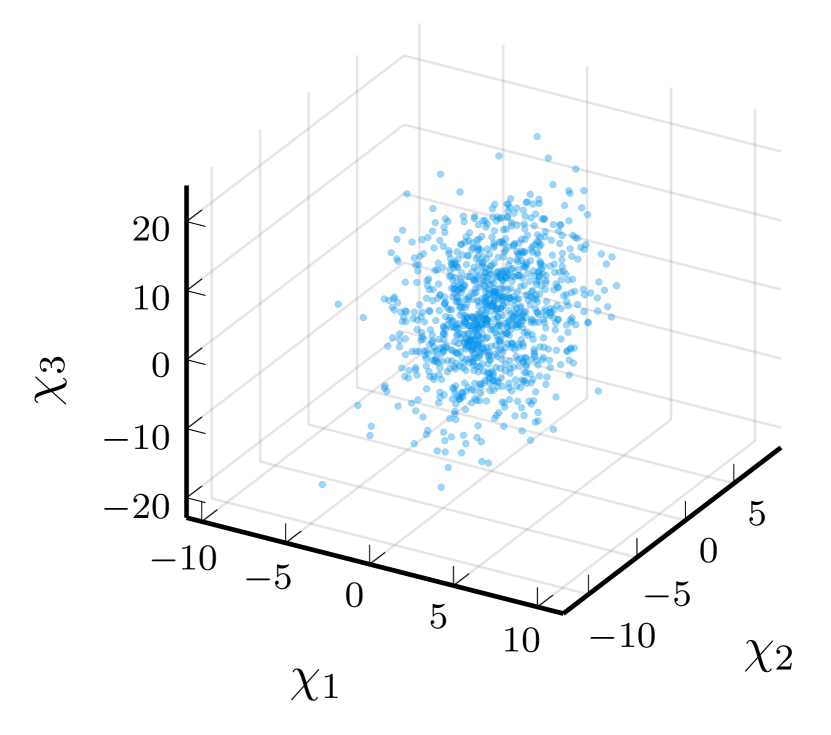
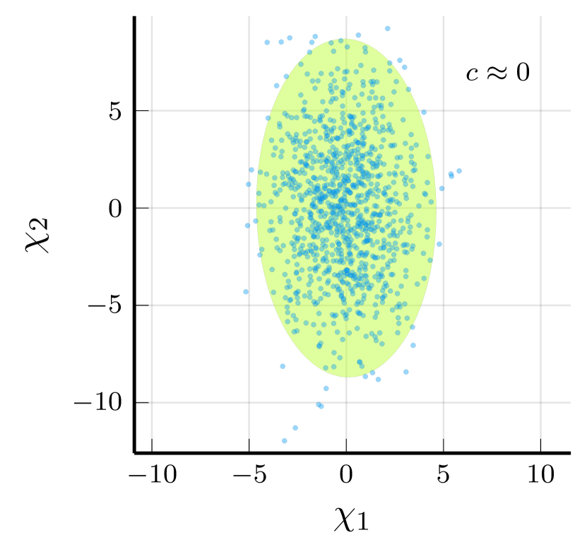
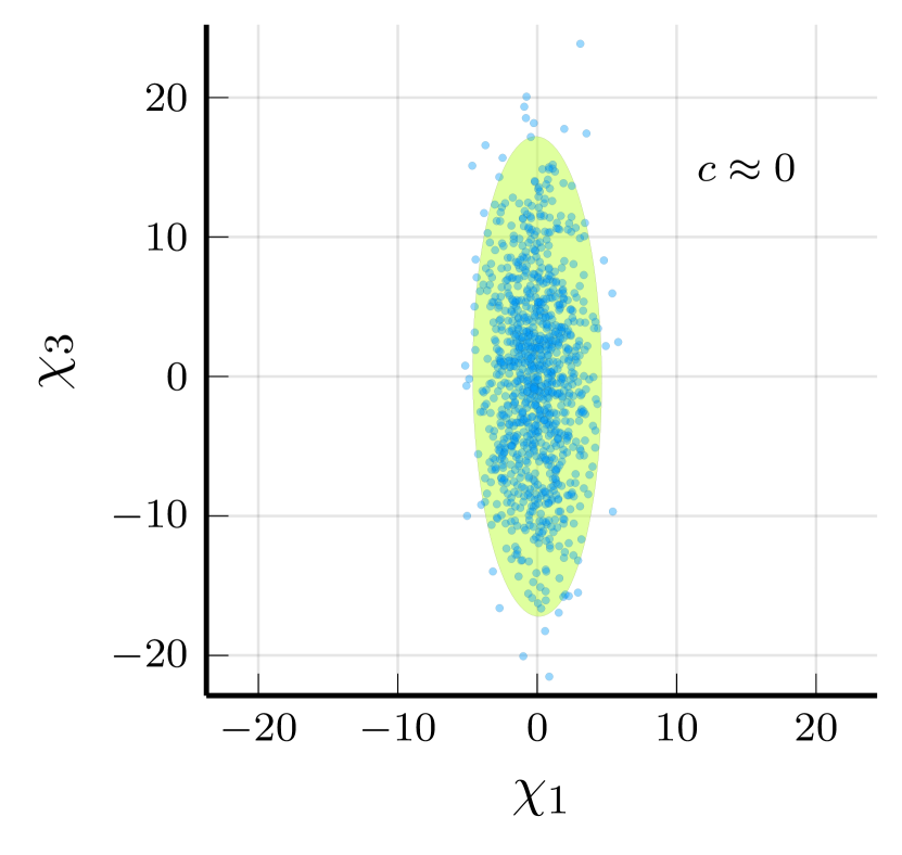
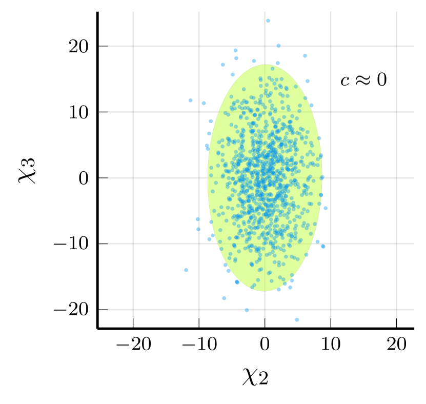
Figure 1: Steady state solution for one thousand instances of model (1) with $A=\operatorname{diag}(-0.54,-0.28,-0.14)$. The computed correlations are close to zero as predicted. Yellow ellipses are covariance ellipses.

III-B Full (anti)correlations in singular 1-dominant networks

Theorem 2

Suppose $A$ has a positive dominant eigenvector $\boldsymbol{v}_{1}$ and associated eigenvalue $\lambda_{1}<0$. Let $\lambda_{2},\ldots,\lambda_{n}$ be the remaining eigenvalues of $A$ satisfying $\mathrm{Re}(\lambda_{i})<\lambda_{1}$, $i=2,\ldots,n$. Then, in the singular limit $\varepsilon=\frac{-1}{\max_{i>1}\{\mathrm{Re}(\lambda_{i})\}}\to 0$ and fixed $\lambda_{1}$, $\operatorname{cor}(\chi_{i},\chi_{j})=1$ for all $i,j\in\{1,\ldots,n\}$ and therefore Problem 1 is unsolvable whenever $c_{i,j}\neq 1$.

Proof:

Let $U$ be the matrix that transforms $A$ in its Jordan canonical form $J$, i.e., $A=UJU^{-1}$, with $J=\begin{bmatrix}\lambda_{1}&0\\ 0&J_{2}\end{bmatrix}$. Let $\tilde{\boldsymbol{x}}=U^{-1}\boldsymbol{x}$. Then,

$$\dot{\tilde{x}}_{1} =\lambda_{1}\tilde{x_{1}}+\langle U^{-1}_{1\cdot},[\xi_{j}]_{j=1}^{n}\rangle,$$ (2)

$$[\dot{\tilde{x}}_{i}]_{i=2}^{n} =J_{2}[x_{j}]_{j=1}^{n}+[\langle U_{i\cdot}^{-1},[\xi_{j}]_{j=1}^{n}\rangle]_{i=1}^{n}\,.$$

It follows along the same lines as [6, Theorem 1] that in the limit $\varepsilon\to 0$, model (2) reduces to the slow dynamics

$$\dot{\tilde{x}}_{1} =\lambda_{1}\tilde{x_{1}}+\langle U^{-1}_{1\cdot},[\xi_{j}]_{j=1}^{n}\rangle,$$

$$\tilde{x}_{i} =0,\quad i=2,\ldots,n\,.$$

Let $\tilde{\chi}_{1}=-\frac{\langle U^{-1}_{1\cdot},[\xi_{j}]_{j=1}^{n}\rangle}{\lambda_{1}}$. Then, in the limit $\varepsilon\to 0$, $\chi_{i}=U_{i1}\tilde{\chi}_{1}$ and therefore, at equibrilium, $\operatorname{cor}(\chi_{i},\chi_{j})=\operatorname{cor}(U_{i1}\tilde{\chi}_{1},U_{j1}\tilde{\chi}_{1})=\frac{\operatorname{cov}(U_{i1}\tilde{\chi}_{1},U_{j1}\tilde{\chi}_{1})}{\sqrt{\operatorname{var}(U_{i1}\tilde{\chi}_{1})\operatorname{var}(U_{j1}\tilde{\chi}_{1})}}=\frac{U_{i1}U_{j1}\operatorname{cov}(\tilde{\chi}_{1},\tilde{\chi}_{1})}{\sqrt{U_{i1}^{2}U_{j1}^{2}\operatorname{var}(\tilde{\chi}_{1})^{2}}}=1$. ∎

Theorem 2 shows that if $A$ has a positive dominant eigenvector with a negative associated eigenvalue $\lambda_{1}$ (e.g., $A$ is Metzler and irreducible [2, Lemma VIII.1] or $A$ is eventually positive [7, Theorem 5]), and if the separation between the slow eigenvalue and the rest of the spectrum is sufficiently large, then all pairs of variables are fully correlated. Figure 2 illustrates this result by simulating one thousand instances of model (1) with $A$ constructed through the inverse of the unitary change of base that diagonalizes it to possess the following (eigenvalue,eigenvector) pairs: $(-0.01,(0.45,0.81,0.36))$, $(-0.2,(-0.81,0.54,-0.2))$, $(-1.0,(-0.36,-0.2,0.9))$. Observe that the resulting equilibrium cloud appears as a three-dimensional ellipse sharply elongated along the dominant (slow) direction because the input-to-state gain along this direction is much larger than along non-dominant ones. Projecting equilibria on the three coordinate planes, the measured correlations are all (close to, due to finite sample size and finite $\varepsilon=0.01$) one.

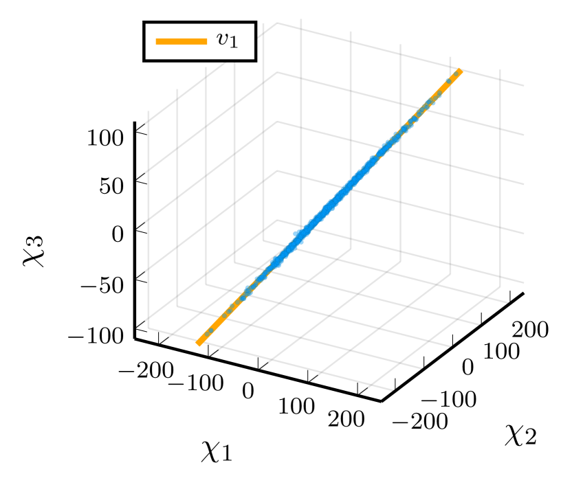
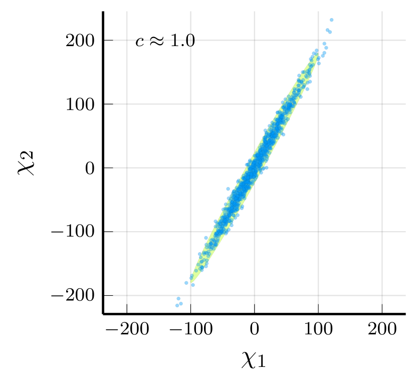
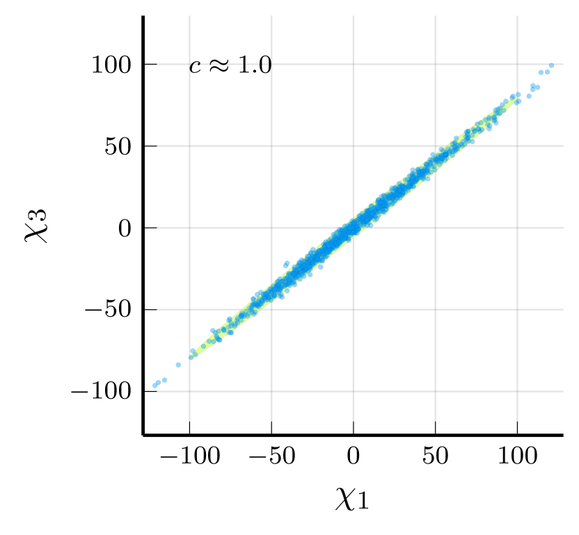
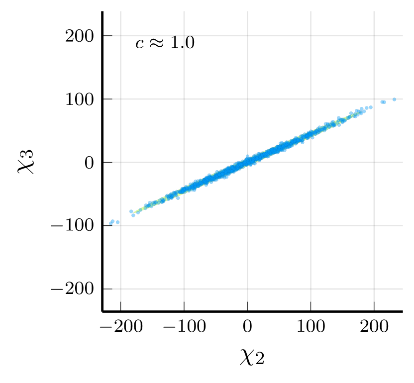
Figure 2: Steady state solution for one thousand instances of model (1) in case $A$ possesses a single dominant direction. The computed correlations are close to one as predicted. Yellow ellipses are covariance ellipses.

Remark 1

For $\epsilon>0$ and sufficiently small, if follows along the same line as [6, Proposition 5], that, $\operatorname{cor}(x_{i}^{*},x_{j}^{*})=1-\mathcal{O}(\varepsilon)$ for all $i,j\in\{1,\ldots,n\}$.

The following theorem addresses the case in which the dominant eigendirection $\boldsymbol{v}_{1}$ has mixed-sign entries. In this case, any pair of variables is either fully correlated or fully anticorrelated.

Theorem 3

Suppose $A$ has a dominant eigendirection $\boldsymbol{v}_{1}$ with associated eigenvalue $\lambda_{1}<0$. Let $\lambda_{2},\ldots,\lambda_{n}$ be the remaining eigenvalues of $A$ satisfying $\mathrm{Re}(\lambda_{i})\ll\lambda_{1}$, $i=2,\ldots,n$. Then, in the singular limit $\varepsilon=\frac{-1}{\max_{i>1}\{\mathrm{Re}(\lambda_{i})\}}\to 0$ and fixed $\lambda_{1}$, $\operatorname{cor}(\chi_{i},\chi_{j})=\operatorname{sgn}([\boldsymbol{v}_{1}]_{i}[\boldsymbol{v}_{1}]_{j})$ for all $i,j\in\{1,\ldots,n\}$ and therefore Problem 1 is unsolvable whenever $c_{i,j}\neq\pm 1$.

Proof:

Follows along the same lines as the proof of Theorem 2 and observing that $U_{i1}=[\boldsymbol{v}_{1}]_{i}$. ∎

IV CORRELATED VARIABILITY CONTROL IN THE PRESENCE OF A REPEATED DOMINANT EIGENVALUE

The results in the Theorems 1 and 2 shows that it should a priori be possible to span the whole range of correlation degrees, from null (no network) to full (strongly 1-dominant network), by suitably changing the network structure. The rationale we follow here is that increasing the dimension of the dominant subspace and designing suitable slow dynamics on it leads a constructive geometric way to solve Problem 1.

IV-A The dominant eigenvalue has algebraic and geometric multiplicity two

Assumption 1

$A$ has a real repeated dominant eigenvalue $\lambda_{1}<0$, with $\gamma_{A}(\lambda_{1})=\mu_{A}(\lambda_{1})=2$, and dominant eigenvectors $\boldsymbol{v}_{1}$ and $\boldsymbol{v}_{2}$. Let $\lambda_{3},\ldots,\lambda_{n}$, $\mathrm{Re}(\lambda_{i})\ll\lambda_{1}$, $i=3,\ldots,n$ be the remaining eigenvalues of $A$.

Lemma 1

Without loss of generality, $\boldsymbol{v}_{1}$ and $\boldsymbol{v}_{2}$ can be taken to be orthonormal.

Proof:

Any vector in $\mathbb{R}\{\boldsymbol{v}_{1},\boldsymbol{v}_{2}\}$ is also an eigenvector of $A$ with eigenvalue $\lambda_{1}$. If not already orthonormal, redefine $\boldsymbol{v}_{1}$ and $\boldsymbol{v}_{2}$ to be an orthonormal basis of $\mathbb{R}\{\boldsymbol{v}_{1},\boldsymbol{v}_{2}\}$. ∎

Lemma 2

There exists is a unitary matrix $Q$ such that $Q^{-1}AQ=\begin{bmatrix}T_{\lambda_{1}}&C\\ 0&B\end{bmatrix}$, where $T_{\lambda_{1}}=\begin{bmatrix}\lambda_{1}&0\\ 0&\lambda_{1}\end{bmatrix}$, $C\in\mathbb{R}^{2,n-2}$, $B\in\mathbb{R}^{n-2,n-2}$, and the eigenvalues of $B$ are exactly $\lambda_{3},\ldots,\lambda_{n}$.

Proof:

Let $\boldsymbol{w}_{3},\boldsymbol{w}_{2},\ldots,\boldsymbol{w}_{n}$ be vectors such that $\{\boldsymbol{v}_{1},\boldsymbol{v}_{2},\boldsymbol{w}_{3},\ldots,\boldsymbol{w}_{n}\}$ is an orthonormal basis of $\mathbb{R}^{n}$ and take $Q$ to be the matrix whose columns are these vectors. Then, $Q$ is unitary. Furthermore, $Q^{-1}AQ=Q^{-1}\begin{bmatrix}\lambda_{1}\boldsymbol{v}_{1}&\lambda_{1}\boldsymbol{v}_{2}&A\boldsymbol{w}_{3}&\cdots&A\boldsymbol{w}_{n}\\ \end{bmatrix}=\left[\begin{array}[]{c|c}\begin{matrix}\lambda_{1}&0\\ 0&\lambda_{1}\end{matrix}&C\\ \hline\cr 0&B\end{array}\right]=\begin{bmatrix}T_{\lambda_{1}}&C\\ 0&B\end{bmatrix}$. To see that the eigenvalues of $B$ are $\lambda_{3},\ldots,\lambda_{n}$, notice that $A$ and $Q^{-1}AQ$ are similar and therefore have the same eigenvalues. ∎

Let $\tilde{x}=Q^{-1}x$. Then,

$$\dot{\tilde{x}}_{1} =\lambda_{1}\tilde{x}_{1}+\langle C_{1\cdot},[\tilde{x}_{j}]_{j=3}^{n}\rangle+\langle Q_{1\cdot}^{-1},[\xi_{j}]_{j=1}^{n}\rangle$$ (3a)

$$\dot{\tilde{x}}_{2} =\lambda_{1}\tilde{x}_{2}+\langle C_{2\cdot},[\tilde{x}_{j}]_{j=3}^{n}\rangle+\langle Q_{2\cdot}^{-1},[\xi_{j}]_{j=1}^{n}\rangle$$ (3b)

$$[\dot{\tilde{x}}_{i}]_{i=3}^{n} =B[\tilde{x}_{j}]_{j=3}^{n}+[\langle Q_{i\cdot}^{-1},[\xi_{j}]_{j=1}^{n}\rangle]_{i=3}^{n}.$$ (3c)

Theorem 4

Under Assumption 1, the slow dynamics of model (1) associated to the singular limit $\varepsilon=\frac{-1}{\max_{i>2}\{\mathrm{Re}(\lambda_{i})\}}\to 0$ and fixed $\lambda_{1}$ of model (3) reads

$$\dot{\tilde{x}}_{1} =\lambda_{1}\tilde{x}_{1}+\langle Q_{1\cdot}^{-1},[\xi_{j}]_{j=1}^{n}\rangle$$ (4a)

$$\dot{\tilde{x}}_{2} =\lambda_{1}\tilde{x}_{2}+\langle Q_{2\cdot}^{-1},[\xi_{j}]_{j=1}^{n}\rangle.$$ (4b)

$$\tilde{x}_{i} =0,\quad i=3,\ldots,n\,.$$ (4c)

Furthermore, the associated critical manifold $\mathcal{M}=\{\tilde{x}_{3}=\cdots=\tilde{x}_{n}=0\}$ is exponentially attractive.

Proof:

Let $B_{1}=\varepsilon B$. Then $B_{1}$ has spectrum $\varepsilon\lambda_{3},\ldots,\varepsilon\lambda_{n}$, with $\varepsilon\max_{i>2}\{\mathrm{Re}(\lambda_{i})\}=-1$. Then (3) becomes

$$\dot{\tilde{x}}_{1} =\lambda_{1}\tilde{x}_{1}+\langle C_{1\cdot},[\tilde{x}_{j}]_{j=3}^{n}\rangle+\langle Q_{1\cdot}^{-1},[\xi_{j}]_{j=1}^{n}\rangle$$ (5)

$$\dot{\tilde{x}}_{2} =\lambda_{1}\tilde{x}_{2}+\langle C_{2\cdot},[\tilde{x}_{j}]_{j=3}^{n}\rangle+\langle Q_{2\cdot}^{-1},[\xi_{j}]_{j=1}^{n}\rangle$$ (6)

$$\varepsilon[\dot{\tilde{x}}_{i}]_{i=3}^{n} =B_{1}[\tilde{x}_{j}]_{j=3}^{n}+\varepsilon[\langle Q_{i\cdot}^{-1},[\xi_{j}]_{j=1}^{n}\rangle]_{i=3}^{n}.$$ (7)

Because $B_{1}$ is Hurwitz and its spectrum is bounded away from zero for all $\varepsilon>0$, in the limit $\varepsilon\to 0$, model (5) reduces to the slow dynamics (4) defined on the critical manifold $\mathcal{M}$, which is also exponentially attractive. ∎

Let $\tilde{\boldsymbol{\chi}}=U^{-1}\chi$. We are now in condition to compute steady-state correlations of model (1).

Theorem 5

Under Assumption 1 and in the singular limit $\varepsilon=\frac{-1}{\max_{i>2}\{\mathrm{Re}(\lambda_{i})\}}\to 0$ and fixed $\lambda_{1}$, equilibria of model (1) satisfy $\operatorname{var}(\tilde{\chi}_{1})=\operatorname{var}(\tilde{\chi}_{2})=\frac{1}{\lambda_{1}^{2}},\ \operatorname{cov}(\tilde{\chi}_{1},\tilde{\chi}_{2})=0$. Furthermore, for all $i,j\in\{1,\ldots,n\}$,

$$\operatorname{cor}(\chi_{i},\chi_{j})=\frac{[\boldsymbol{v}_{1}]_{i}[\boldsymbol{v}_{1}]_{j}+[\boldsymbol{v}_{2}]_{i}[\boldsymbol{v}_{2}]_{j}}{\sqrt{([\boldsymbol{v}_{1}]_{i}^{2}+[\boldsymbol{v}_{2}]_{i}^{2})([\boldsymbol{v}_{1}]_{j}^{2}+[\boldsymbol{v}_{2}]_{j}^{2})}}.$$ (8)

Proof:

Observe that $\tilde{\chi}_{1}=-\frac{\langle Q_{1\cdot}^{-1},[\xi_{j}]_{j=1}^{n}\rangle}{\lambda_{1},},\ \tilde{\chi}_{2}=-\frac{\langle Q_{2\cdot}^{-1},[\xi_{j}]_{j=1}^{n}\rangle}{\lambda_{1}}$. Using the facts that $\operatorname{cov}(\xi_{i},\xi_{j})=\delta_{ij}$ and that the covariance function is bilinear, we have $\operatorname{cov}(\tilde{\chi}_{j},\tilde{\chi}_{l})=\frac{1}{\lambda_{1}^{2}}\sum_{k=1}^{n}Q_{jk}^{-1}Q_{lk}^{-1},\ j,l=1,2$. The formulas for $\operatorname{var}(\tilde{\xi}_{j})$ and $\operatorname{cov}(\tilde{\chi}_{j},\tilde{\chi}_{l})$, $j,l=1,2$, then follow by recalling that, by Lemma 2, $Q_{j\cdot}^{-1}=\boldsymbol{v}_{j}$, $j=1,2$, and that, by Lemma 1, $\boldsymbol{v}_{1}$ and $\boldsymbol{v}_{2}$ are orthonormal. The formulas for $\operatorname{cor}(\chi_{i},\chi_{j})$ follow by invoking Theorem 4, which implies that in the limit $\varepsilon\to 0$, $\chi_{i}=[\boldsymbol{v}_{1}]_{i}\tilde{\chi}_{1}+[\boldsymbol{v}_{2}]_{i}\tilde{\chi}_{2}$. ∎

Theorem 5 shows that, under Assumption 1 and in the singular limit of strong dominance $\varepsilon\to 0$, the $n$-dimensional covariance ellipse generated by the steady states of model (1) reduces to a (two-dimensional) circle of radius $|\lambda_{1}|^{-1}$ on the dominant subspace spanned by $\boldsymbol{v}_{1}$ and $\boldsymbol{v}_{2}$. Furthermore it provides explicit formulas (8) in terms of the components of the dominant eigenvectors $\boldsymbol{v}_{1}$ and $\boldsymbol{v}_{2}$ for the steady-state correlations $\operatorname{cor}(\chi_{i},\chi_{j})$.

Expressions (8) can be plugged into out-of-the-box optimization software to find solutions to Problem 1 but still provide no guarantees about the existence of such solutions nor about the geometry of the possible solution set. We have the following theorem.

Theorem 6

Let Assumption 1 be satisfied and let $n=3$. Then, in the limit $\varepsilon=\frac{-1}{\max_{i>1}\{\mathrm{Re}(\lambda_{i})\}}\to 0$ and fixed $\lambda_{1}$, Problem 1 has solution on an open set of desired correlations $c_{1,2},c_{2,3},c_{1,3}$. Furthermore, when they exist, solutions are isolated.

Proof:

Observe that because $\boldsymbol{v}_{1}$ and $\boldsymbol{v}_{2}$ are orthonormal, for $n=3$ they are parameterized by three angles $\theta_{1},\theta_{2},\theta_{3}$ (e.g., the two angles defining the orientation of $\boldsymbol{v}_{1}$ and the angle of $\boldsymbol{v}_{2}$ on the plan orthogonal to $\boldsymbol{v}_{1}$). Under this parameterization, (8) defines a smooth map

$$\Phi:\mathbb{R}^{3} \to\mathbb{R}^{3}$$

$$(\theta_{1},\theta_{2},\theta_{3}) \mapsto(\operatorname{cor}(\chi_{1},\chi_{2}),\operatorname{cor}(\chi_{2},\chi_{3}),\operatorname{cor}(\chi_{3},\chi_{1})).$$

Furthermore, observe that $\Phi$ has range $[-1,1]^{3}$ and therefore, for $n=3$, there exists at least one combination of desired correlations for which Problem 1 has solution. It is lengthy but straightforward to show that the Jacobian of $\Phi$ is non-singular almost everywhere and therefore by the Open Mapping theorem [4] its image is open. Thus, Problem 1 has a solution on an open set of desired correlations, i.e., the image of $\Phi$. Let $c_{1,2},c_{2,3},c_{1,3}$ be desired correlations for which a solution to Problem 1 exist. Let $\Phi_{1,2}(\theta_{1},\theta_{2},\theta_{3})=\operatorname{cor}(\chi_{1},\chi_{2})$ be the first component of $\Phi$. By the Implicit Function theorem applied to $\Phi_{1,2}$, there exists a two-dimensional almost-everywhere (i.e., except at possible singularities) smooth manifold $\mathcal{M}_{1,2}\subset\mathbb{R}^{3}$ such that if $\Phi_{1,2}(\theta_{1},\theta_{2},\theta_{3})=c_{1,2}$, then $(\theta_{1},\theta_{2},\theta_{3})\in\mathcal{M}_{1,2}$. Through the same argument, it follows that simulataneously imposing $\operatorname{cor}(\chi_{1},\chi_{2})=c_{1,2}$, $\operatorname{cor}(\chi_{2},\chi_{3})=c_{2,3}$, and $\operatorname{cor}(\chi_{3},\chi_{1})=c_{3,1}$ implies $(\theta_{1},\theta_{2},\theta_{3})\in\mathcal{M}_{1,2}\cap\mathcal{M}_{2,3}\cap\mathcal{M}_{3,1}$, where $\mathcal{M}_{2,3},\mathcal{M}_{3,1}$ are also two-dimensional almost-everywhere smooth manifolds. Recalling that the intersection of three two-dimensional manifold in $R^{3}$ is generically zero-dimensional, i.e, made of isolated points, the result follows. ∎

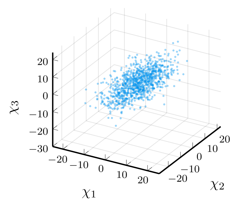
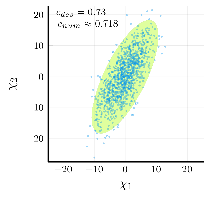
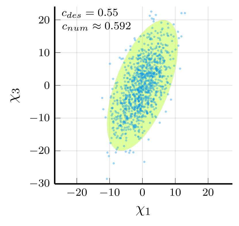
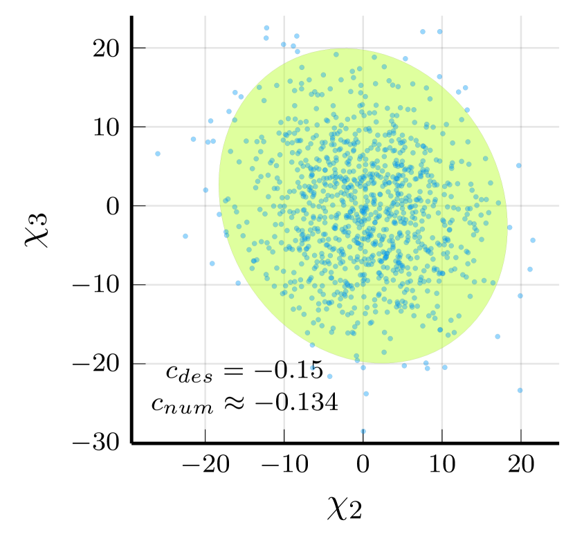
Figure 3: Steady state solution for one thousand instances of model (1) in case the dominant eigenvalue of $A$ has algebraic and geometric multiplicity two. The computed correlations are close to the desired control values. Yellow ellipses are covariance ellipses.

Figure 3 illustrates Theorem 6. An orthonormal solution $\boldsymbol{v}_{1},\boldsymbol{v}_{2}$ to Problem 1 was found by plugging expression (8) into the Julia Optimization package Optim.jl [10]. Given this solution, we assigned $\lambda_{1}=-0.01$ and $\lambda_{3}=-1.0$. The eigenvector $\boldsymbol{v}_{3}$ associated to $\lambda_{3}$ was taken to be orthonormal to $\boldsymbol{v}_{1},\boldsymbol{v}_{2}$. The Hurwitz matrix $A$ was then constructed through the inverse of the unitary change of base associated to the base $\boldsymbol{v}_{1},\boldsymbol{v}_{2},\boldsymbol{v}_{3}$. We then simulated one-thousand instances of model (1). As shown in Figure 3 numerically computed correlations are close to the associated desired control values. To verify that the solution set is indeed made of isolated points we rerun our algorithm for the same desired correlation values as Figure 3 but let the optimization procedure converge to a new solution for five hundred initial conditions in a small neighborhood of the solution corresponding to Figure 3. The result of this experiment is reproduced in Figure 5 (yellow plots). The optimizer consistently converges back to the original solution, which, as predicted by Theorem 6, shows that no other solutions exist close to it.

IV-B The dominant eigenvalue has algebraic multiplicity two but geometric multiplicity one

We develop this section under the following assumption.

Assumption 2

$A$ has a real repeated dominant eigenvalue $\lambda_{1}<0$, with $\gamma_{A}(\lambda_{1})=1$, $\mu_{A}(\lambda_{1})=2$, dominant normalized eigenvector $\boldsymbol{v}_{1}$ and generalized normalized eigenvector $\boldsymbol{v}_{2}$. Let $\lambda_{3},\ldots,\lambda_{n}$, $\mathrm{Re}(\lambda_{i})\ll\lambda_{1}$, $i=3,\ldots,n$ be the remaining eigenvalues of $A$.

Let $U$, with $U_{\cdot 1}=\boldsymbol{v}_{1}$ and $U_{\cdot 2}=\boldsymbol{v}_{2}$, be the matrix that transforms $A$ in its Jordan canonical form $J$, i.e., $A=UJU^{-1}$, with $J=\begin{bmatrix}J_{\lambda_{1}}&0\\ 0&J_{2}\end{bmatrix}$, where $J_{\lambda_{1}}$ is the two-dimensional Jordan block associated to $\lambda_{1}$ and $J_{2}$ contains Jordan blocks $\lambda_{3},\ldots,\lambda_{n}$. Let $\tilde{x}=U^{-1}x$. Then

$$\begin{split}\dot{\tilde{x}}_{1}&=\lambda_{1}\tilde{x}_{1}+\tilde{x}_{2}+\langle U_{1\cdot}^{-1},[\xi_{j}]_{j=1}^{n}\rangle,\\ \dot{\tilde{x}}_{2}&=\lambda_{1}\tilde{x}_{2}+\langle U_{2\cdot}^{-1},[\xi_{j}]_{j=1}^{n}\rangle,\\ [\dot{\tilde{x}}_{i}]_{i=3}^{n}&=J_{2}[\tilde{x}_{j}]_{j=3}^{n}+[\langle U_{i\cdot}^{-1},[\xi_{j}]_{j=1}^{n}\rangle]_{i=3}^{n}.\end{split}$$ (9)

The proof of the following theorem follows along the same line as the proof of Theorem 4.

Theorem 7

Under Assumption 2, the slow dynamics of model (1) associated to the singular limit $\varepsilon=\frac{-1}{\max_{i>2}\{\mathrm{Re}(\lambda_{i})\}}\to 0$ and fixed $\lambda_{1}$ of model (3) reads

$$\dot{\tilde{x}}_{1} =\lambda_{1}\tilde{x}_{1}+\tilde{x}_{2}+\langle U_{1\cdot}^{-1},[\xi_{j}]_{j=1}^{n}\rangle,$$

$$\dot{\tilde{x}}_{2} =\lambda_{1}\tilde{x}_{2}+\langle U_{2\cdot}^{-1},[\xi_{j}]_{j=1}^{n}\rangle,$$

$${\tilde{x}}_{i} =0,\quad i=1,\ldots,n\,.$$

Furthermore, the associated critical manifold $\mathcal{M}=\{\tilde{x}_{3}=\cdots=\tilde{x}_{n}=0\}$ is exponentially attractive.

Let $\tilde{\boldsymbol{\chi}}=U^{-1}\chi$. We are now in condition to compute steady-state correlations of model (1).

Theorem 8

Under Assumption 2 and in the singular limit $\varepsilon=\frac{-1}{\max_{i>2}\{\mathrm{Re}(\lambda_{i})\}}\to 0$ and fixed $\lambda_{1}$, equilibria of model (1) satisfy

$$\operatorname{var}({\tilde{\chi}_{1}})\!=\!\sum_{i=1}^{n}\!\bigg{(}\!\frac{-\lambda_{1}U_{1i}^{-1}\!+\!U_{2i}^{-1}}{\lambda_{1}^{2}}\bigg{)}^{2}\!\!\!,\operatorname{var}({\tilde{\chi}_{2}})\!=\!\sum_{i=1}^{n}\!\bigg{(}\!\!-\frac{U_{2i}^{-1}}{\lambda_{1}}\bigg{)}^{2}$$

$$\operatorname{cov}({\tilde{\chi}_{1}},{\tilde{\chi}_{2}})=-\frac{1}{\lambda_{1}^{3}}\sum_{i=1}^{n}(-\lambda_{1}U_{1i}^{-1}+U_{2i}^{-}1)(U_{2i}^{-1}).$$

Furthermore, for all $i,j\in\{1,\ldots,n\}$,

$$\operatorname{cor}(\chi_{i},\chi_{j})=\frac{\beta_{1}}{\sqrt{\beta_{2}\cdot\beta_{3}}}$$ (11)

where $\beta_{1}=[\boldsymbol{v}_{1}]_{i}[\boldsymbol{v}_{1}]_{j}\operatorname{var}(\tilde{\chi}_{1})+([\boldsymbol{v}_{1}]_{i}[\boldsymbol{v}_{2}]_{j}+[\boldsymbol{v}_{2}]_{i}[\boldsymbol{v}_{1}]_{j})\operatorname{cov}(\tilde{\chi}_{1},\tilde{\chi}_{2})+[\boldsymbol{v}_{2}]_{i}[\boldsymbol{v}_{2}]_{j}\operatorname{var}(\tilde{\chi}_{2})$, $\beta_{2}=[\boldsymbol{v}_{1}]_{i}^{2}\operatorname{var}(\tilde{\chi}_{1})+[\boldsymbol{v}_{2}]_{i}^{2}\operatorname{var}(\tilde{\chi}_{2})+2[\boldsymbol{v}_{1}]_{i}[\boldsymbol{v}_{2}]_{i}\operatorname{cov}(\tilde{\chi}_{1},\tilde{\chi}_{2})$, $\beta_{3}=[\boldsymbol{v}_{1}]_{j}^{2}\operatorname{var}(\tilde{\chi}_{1})+[\boldsymbol{v}_{2}]_{j}^{2}\operatorname{var}(\tilde{\chi}_{2})+2[\boldsymbol{v}_{1}]_{j}[\boldsymbol{v}_{2}]_{j}\operatorname{cov}(\tilde{\chi}_{1},\tilde{\chi}_{2})$.

Proof:

The first part of the statement follows by solving for the steady-states of the slow dynamics (10) and using properties of the covariance function along the same lines as the proof of Theorem 5. The formulas for $\operatorname{cor}(\chi_{i},\chi_{j})$ follow by invoking Theorem 7, which implies that in the limit $\varepsilon\to 0$, $\chi_{i}=[\boldsymbol{v}_{1}]_{i}\tilde{\chi}_{1}+[\boldsymbol{v}_{2}]_{i}\tilde{\chi}_{2}$. ∎

To study the geometry of the solution set of Problem 1 under Assumption 2 and for $n=3$, we follow the same steps as for Theorem 6. The key point is observing that in solving $\operatorname{cor}(\chi_{i},\chi_{j})=c_{i,j}$, with $\operatorname{cor}(\chi_{i},\chi_{j})$ defined by (11), for $n=3$ there are five independent variables, that is, the two solid angles $((\theta_{1},\theta_{2}),(\theta_{3},\theta_{4}))$, which define the two normalized vectors $\boldsymbol{v}_{1},\boldsymbol{v}_{2}$, and the slow eigenvalue $\lambda_{1}$. Hence, imposing values for the three correlations leads to a solution set given by the intersection of three four-dimensional manifolds in $\mathbb{R}^{5}$, i.e., in general, a two-dimensional manifold.

Theorem 9

Let Assumption 2 be satisfied and let $n=3$. Then, in the limit $\varepsilon=\frac{-1}{\max_{i>1}\{\mathrm{Re}(\lambda_{i})\}}\to 0$ and fixed $\lambda_{1}$, Problem 1 has solution on an open set of desired correlations $c_{1,2},c_{2,3},c_{1,3}$. Furthermore, when they exist, solutions lies on a two-dimensional manifold.

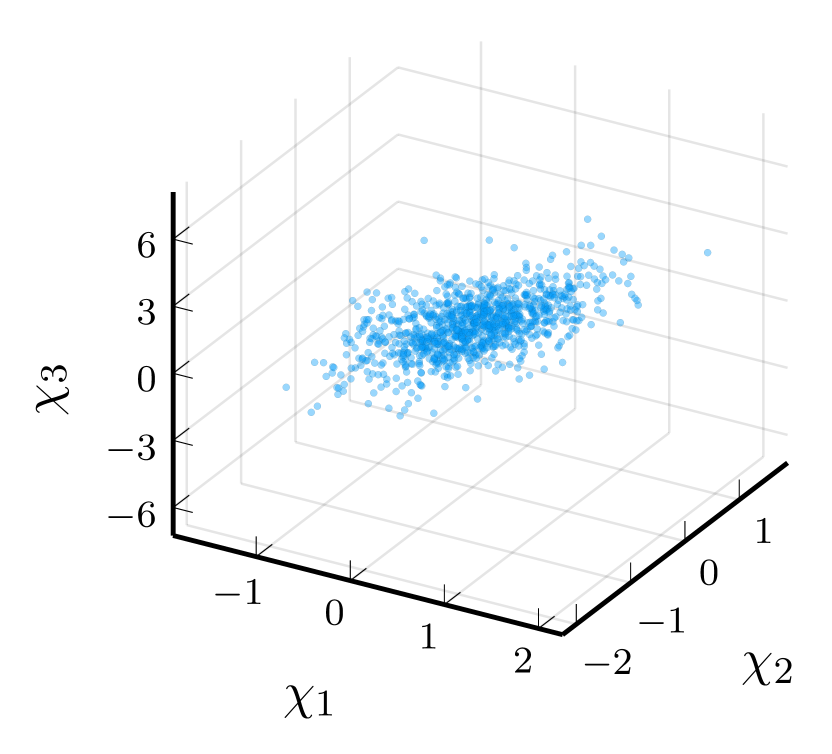
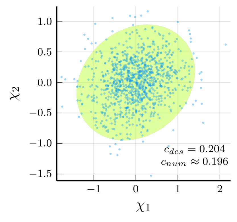
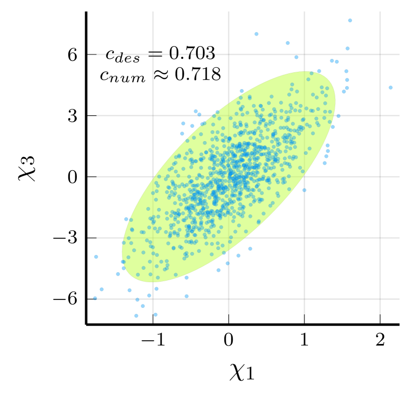
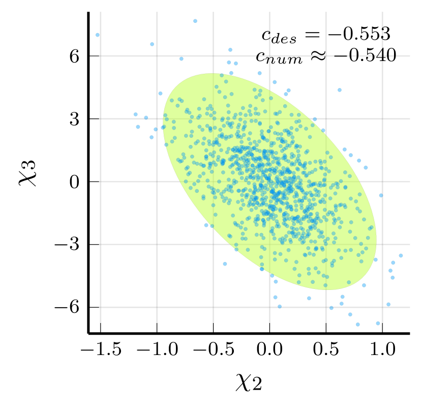
Figure 4: Steady state solution for one thousand instances of model (1) in case the dominant eigenvalue of $A$ has algebraic multiplicity two but geometric multiplicity one. The computed correlations are close to the desired control values. Yellow ellipses are covariance ellipses.

Figure 4 illustrates Theorem 6. A solution to Problem 1 was found by plugging expression (11) into the Julia Optimization package Optim.jl [10]. In our algorithm, the third eigenvector $\boldsymbol{v}_{3}$ of matrix $A$, which is needed to define the matrix $U$ and its inverse, was defined as the unitary norm vector orthogonal to $\mathbb{R}\{\boldsymbol{v}_{1},\boldsymbol{v}_{2}\}$. The solution of our optimization procedure is the pair $\boldsymbol{v}_{1},\boldsymbol{v}_{2}$ (and hence the orthonormal vector $\boldsymbol{v}_{3}$) and the slow eigenvalue $\lambda_{1}$. Given this solution, we assigned $\lambda_{3}=100\lambda_{1}$. The Hurwitz matrix $A$ was then constructed through the inverse of the change of base associated to the base $\boldsymbol{v}_{1},\boldsymbol{v}_{2},\boldsymbol{v}_{3}$. We then simulated one-thousand instances of model (1). As shown in Figure 4 numerically computed correlations are close to the associated desired control values. To verify that the solution set indeed lies on a two-dimensional manifold, we rerun our algorithm for the same desired correlation values as Figure 4 but letting the optimization procedure converge to a new solution for five hundred initial conditions in a small neighborhood of the solution corresponding to Figure 4. The result of this experiment is reproduced in Figure 5 (blue plots). The optimizer converged to disparate solutions. The dimension of the resulting set of solution was approximated via Principal Component Analysis using the package Julia MultivariateStats.jl. As shown in Figure 6, only two dimensions consistently capture almost 100% of the variance of the solution set, confirming Theorem 9.

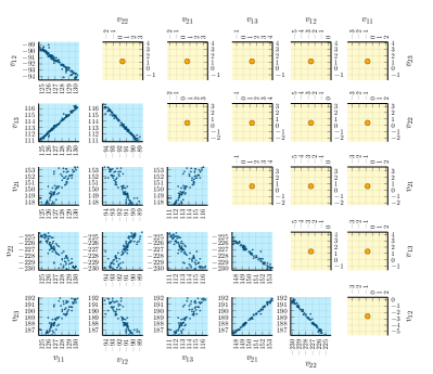
Figure 5: Projection of the components of the solution vectors $\boldsymbol{v}_{1}$ and $\boldsymbol{v}_{2}$ to Problem 1 for the same cases as Figure 3 (yellow) and Figure 4 (blue) when the optimization algorithm is initialized close to the solution of the respective figure.

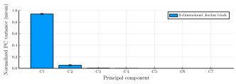
Figure 6: Principal component analysis (variance captured by the various components) of the solution set in Figure 5.

V Discussion

Correlated variability is a fundamental property of biological neural systems but our understanding of it is still very poor. We introduced a control theoretical control problem that might lead to new insights about the functions and origins of correlated variability. The solution to this problem we started to sketch already revealed clear geometric connections between correlated variability and network structure. From a purely mathematical perspective, our work opens the question of which network structure implies two-dimensional dominant dynamics with geometric multiplicity one or two, in the same way as Metzler or eventually positive interconnection matrices lead to one-dominant dynamics.

References

- [1] L. F. Abbott and P. Dayan, “The effect of correlated variability on the accuracy of a population code,” Neural computation, vol. 11, no. 1, pp. 91–101, 1999.
- [2] D. Angeli and E. D. Sontag, “Monotone control systems,” IEEE Transactions on automatic control, vol. 48, no. 10, pp. 1684–1698, 2003.
- [3] B. B. Averbeck, P. E. Latham, and A. Pouget, “Neural correlations, population coding and computation,” Nature reviews neuroscience, vol. 7, no. 5, pp. 358–366, 2006.
- [4] R. Bartle, The Elements of Real Analysis. Wiley, 1976.
- [5] R. Durrett, Probability: theory and examples. Cambridge university press, 2019, vol. 49.
- [6] A. Franci, T. O’Leary, and J. Golowasch, “Positive dynamical networks in neuronal regulation: How tunable variability coexists with robustness,” IEEE Control Systems Letters, vol. 4, no. 4, pp. 946–951, 2020.
- [7] G. Giordano and C. Altafini, “Interaction sign patterns in biological networks: from qualitative to quantitative criteria,” in 2017 IEEE 56th Annual Conference on Decision and Control (CDC). IEEE, 2017, pp. 5348–5353.
- [8] A. Kohn, R. Coen-Cagli, I. Kanitscheider, and A. Pouget, “Correlations and neuronal population information,” Annual review of neuroscience, vol. 39, pp. 237–256, 2016.
- [9] M. L. Leavitt, F. Pieper, A. J. Sachs, and J. C. Martinez-Trujillo, “Correlated variability modifies working memory fidelity in primate prefrontal neuronal ensembles,” Proceedings of the National Academy of Sciences, vol. 114, no. 12, pp. E2494–E2503, 2017.
- [10] P. K. Mogensen and A. N. Riseth, “Optim: A mathematical optimization package for Julia,” Journal of Open Source Software, vol. 3, no. 24, p. 615, 2018.
- [11] V. Pernice and R. A. da Silveira, “Interpretation of correlated neural variability from models of feed-forward and recurrent circuits,” PLoS computational biology, vol. 14, no. 2, p. e1005979, 2018.
- [12] D. J. Schulz, J.-M. Goaillard, and E. E. Marder, “Quantitative expression profiling of identified neurons reveals cell-specific constraints on highly variable levels of gene expression,” Proceedings of the National Academy of Sciences, vol. 104, no. 32, pp. 13 187–13 191, 2007.
- [13] T. Tran, C. T. Unal, D. Severin, L. Zaborszky, H. G. Rotstein, A. Kirkwood, and J. Golowasch, “Ionic current correlations are ubiquitous across phyla,” Scientific reports, vol. 9, no. 1, pp. 1–9, 2019.