Scheduler-Pointed False Data Injection Attack for Event-Based Remote State Estimation

Abstract

In this paper, an attack problem is investigated for event-based remote state estimation in cyber-physical systems. Our objective is to degrade the effect of the event-based scheduler while bypassing a $\chi^{2}$ false data detector. A two-channel scheduler-pointed false data injection attack strategy is proposed by modifying the numerical characteristics of innovation signals. The attack strategy is proved to be always existent, and an algorithm is provided to find it. Under the proposed attack strategy, the scheduler becomes almost invalid and the performance of the remote estimator is degraded. Numerical simulations are used to illustrate our theoretical results.

, ,

1 Introduction

Recently, the security problem of cyber-physical systems (CPSs) has attracted great attention. Successful attacks lead to a variety of serious consequences, such as negative impact on economy, national security and even human lives[1]. The existing attack strategies can be roughly classified into two groups: denial-of-service (DoS) attacks and deception attacks. DoS attacks aim to violate data availability through obstructing the transmission of information flows [2]. Deception attacks affect the integrity of the transmitted data while remaining stealthy to the anomaly detection [3]. Compared with DoS attacks, deception attacks are more energy-saving and stealthy, and fit the aim of malicious agents[4].

Deception attacks have recently received much attention, and can be divided into two types. The first one is called reply attack where sensor data are recorded and replayed without system knowledge. The feasibility problem was studied for control systems equipped with false-data detectors[5] and a countermeasure was proposed in [6] to detect such an attack. The second is called false-data injection (FDI) attack where system knowledge is required. The idea of FDI attack is initially proposed in [3] for power network systems. In [7], an optimal linear FDI attack strategy was designed for remote state estimation problems. A two-channel attack strategy was proposed to handle more general situations in [8]. The authors of [9] considered a stealthy attack, which could drive the system state to some other target states instead of driving to infinity in the most of existing results[10].

In CPSs, both packet dropout and event-based schedulers are common for the communication networks. As a result, the sensor-to-estimator communication rate is not $100\%$ and the above results[7, 8, 9, 10] become no longer applicable. For example, the strategies in [9, 10] are based on idealistic communication channels. Naturally, an interesting topic is to consider FDI attack problem in more realistic situations.

In this paper, we propose a new type of FDI attack strategy for remote state estimation problem with an event-based data scheduler. In practice, event-based schedulers are widely used to reduce communication rate for saving energy[6] or sparing transmission bandwidth[11]. For example, a event-based scheduler for remote state estimation was proposed in [12], where the sensor schedule was determined by innovation of Kalman filters. Our work aims at injecting false data to degrade the event-based scheduler without being detected by a false data detector at the remote state estimator. We propose a two-channel scheduler-pointed FDI attack strategy. In the forward channel, the innovation sequence is attacked through scaling up the mean to trigger the scheduler while squeezing the variance to bypass the detector. In the feedback channel, the feedback data is modified to guarantee the effect of the forward attack. The existence of our attack strategy is proved by characteristics of Gaussian distribution, and the feasible set of all attack parameters can be found analytically. We also analyzed the performance evolution of the remote estimator under this type of attacks. Our result shows that a successful attack strategy can always be designed such that the event-based scheduler becomes almost invalidated and the estimation performance is degraded simultaneously. Finally, a numerical example is presented to illustrate the efficiency of the attack strategy.

Notation: $\mathbb{N}$ and $\mathbb{R}$ denote the sets of natural numbers and real numbers, respectively. $\mathbb{R}^{n}$ is the $n$-dimensional Euclidean space. $\mathbb{S}_{+}^{n}$ is the set of $n\times n$ positive semi-definite matrices. When $X\in\mathbb{S}_{+}^{n}$, we simply write $X\geq 0$; Similarly, $X\geq Y$ means $X-Y\geq 0$. $\mathcal{N}(\mu,\Sigma)$ denotes Gaussian distribution with mean $\mu$ and covariance matrix $\Sigma$. $\mathbf{E}[\cdot]$ denotes the mathematical expectation and $\mathrm{Pr}(\cdot)$ denotes the probability of a random event. $\mathrm{Tr}\{\cdot\}$ denotes the trace of a matrix and the superscript “${\top}$” stands for transposition. $I_{n}$ is the $n\times n$-dimensional identity matrix. The term $xx^{\top}$ for vector $x$ is abbreviated as $x(*)^{\top}$.

2 Preliminaries and Problem Formulation

This section firstly describes the model of an event-based remote state estimator as shown in Fig. 1. A two-channel scheduler-pointed FDI attack strategy is then formulated.

2.1 Process Model

The physical plant in Fig. 1 is described by a discrete time linear time-invariant process

$$x_{k+1} =Ax_{k}+w_{k}$$ (1)

$$y_{k} =Cx_{k}+v_{k}$$ (2)

where $k\in\mathbb{N}$ is the time index, $x_{k}\in\mathbb{R}^{n}$ is the vector of system states, $y_{k}\in\mathbb{R}^{m}$ is the vector of sensor measurements, $w_{k}\in\mathbb{R}^{n}$ and $v_{k}\in\mathbb{R}^{m}$ are zero-mean i.i.d. Gaussian noises with covariances $Q\geq 0$ and $R>0,$ respectively. The initial state $x_{0}$ is zero-mean Gaussian with covariance $\Xi_{0}\geq 0$, and is independent of $w_{k}$ and $v_{k}$ for all $k\geq 0.$ The pair $(A,C)$ is detectable and $(A,\sqrt{Q})$ is stabilizable.

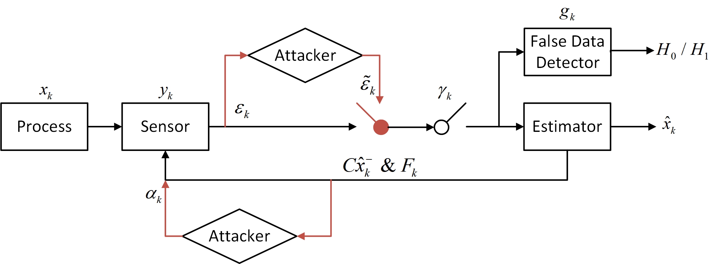
Figure 1: System block diagram.

2.2 Event-Based Remote Estimator

Based on sensor data and estimator feedback data, an event-based scheduler and the corresponding approximate minimum mean-squared error (MMSE) estimator are shown as follows[12]:

• Time update:

  $$\left\{\begin{aligned} \hat{x}_{k}^{-}&=A\hat{x}_{k-1}\\ P_{k}^{-}&=h\left(P_{k-1}\right)\end{aligned}\right.$$ (3)

  where

  $$h(X)\triangleq AXA^{\top}+Q.$$ (4)

  The estimates $\hat{x}_{k}^{-}$ and $\hat{x}_{k}$ here are a priori and a posteriori MMSE estimate, respectively; and the matrices $P_{k}^{-}$ and $P_{k}$ are the corresponding error covariances.

• Measurement update:

  $$\left\{\begin{aligned} \hat{x}_{k}&=\hat{x}_{k}^{-}+\gamma_{k}K_{k}z_{k}\\ K_{k}&=P_{k}^{-}C^{\top}\left[CP_{k}^{-}C^{\top}+R\right]^{-1}\\ P_{k}&=\gamma_{k}\tilde{q}\left(P_{k}^{-}\right)+\left(1-\gamma_{k}\right)\tilde{q}_{\kappa(\beta)}\left(P_{k}^{-}\right)\end{aligned}\right.$$ (5)

  where $z_{k}$ is the measurement innovation, $\gamma_{k}$ is the binary decision variable indicating whether the event-based scheduler shall be closed ($\gamma_{k}=1$) or open ($\gamma_{k}=0$), $K_{k}$ is the standard Kalman gain, and

  $$\tilde{q}_{\lambda}(X) \triangleq X-\lambda XC^{\top}\left[CXC^{\top}+R\right]^{-1}CX$$ (6)

  $$\kappa(\beta) =\frac{2}{\sqrt{2\pi}}\beta e^{-\frac{\beta^{2}}{2}}[1-2Q(\beta)]^{-1}$$ (7)

  if $\lambda=1$, $\tilde{q}_{\lambda}$ will be written as $\tilde{q}$ for brevity. $Q(\cdot)$ is the standard $Q$-function defined by

  $$Q(\beta)\triangleq\int_{\beta}^{+\infty}\frac{1}{\sqrt{2\pi}}e^{-\frac{x^{2}}{2}}\mathrm{d}x.$$ (8)

• Mahalanobis transformation matrix:
  Due to $CP_{k}^{-}C^{\top}+R>0,$ there exists an invertible matrix $F_{k}\in\mathbb{R}^{m\times m}$ such that

  $$F_{k}F_{k}^{\top}=\left(CP_{k}^{-}C^{\top}+R\right)^{-1}.$$

  Based on the raw measurement data $y_{k}$, the feedback data $C\hat{x}_{k}^{-}$ and $F_{k}$, the sensor calculates the innovation

  $$z_{k}=y_{k}-C\hat{x}_{k}^{-}$$ (9)

  where $z_{k}\sim\mathcal{N}(0,CP_{k}^{-}C^{\top}+R)$[6]. Then the innovation’s Mahalanobis transformation

  $$\epsilon_{k}\triangleq F_{k}^{\top}z_{\mathrm{k}}$$ (10)

  is sent to the event-based scheduler. Note that $\epsilon_{k}\sim\mathcal{N}(0,I_{m})$.

The event-based scheduler works as follows:

$$\gamma_{k}=\left\{\begin{array}[]{ll}0,&\text{ if }\left\|\epsilon_{k}\right\|_{\infty}\leq\beta\\ 1,&\text{ otherwise }\end{array}\right.$$ (11)

where $\beta\geq 0$ is a fixed threshold.

2.3 False-Data Detector

At time $k$, the system utilizes a $\chi^{2}$ failure detector by checking the following hypothesis test:

$$g_{k}=z_{k}^{\top}\left(CP_{k}^{-}C^{\top}+R\right)^{-1}z_{k}=\epsilon_{k}^{\top}\epsilon_{k}\underset{H_{1}}{\overset{H_{0}}{\lessgtr}}\sigma$$ (12)

where the null hypothesis $H_{0}$ means that the system is operating normally, while the alternative hypothesis $H_{1}$ means that the system is under attack. When $H_{1}$ happens, an alarm will be launched. Note that $g_{k}$ is $\chi^{2}$ distributed with $m$ degrees of freedom.

Because $g_{k}\geq\left\|\epsilon_{k}\right\|_{\infty}^{2}$, it is necessary to require that $\beta<\sqrt{\sigma}$ to avoid the alarm being activated whenever the event-based scheduler is triggered in view of (11).

Remark 1.

In practice, the threshold $\sigma$ could be designed corresponding to an acceptable false alarm rate $\Upsilon$, i.e., $\Pr(g_{k}\geq\sigma)=\Upsilon$, see Definition 1 in the following.

2.4 Attack Model

To launch attacks, the following assumptions are required over the communication channels.

Assumption 2.

The attacker knows all the system parameters, e.g., $A$, $C$, $Q$, $R$ and $K$.

Assumption 3.

The attacker can modify the data transmitted through the forward and feedback channels.

As shown in Fig. 1, we launch two attacks at both forward and feedback communication channels.

The converted innovation data $\epsilon_{k}$ is modified by the forward channel attacker as follows

$$\tilde{\epsilon}_{k}=\frac{1}{\mu_{k}}\epsilon_{k}+\delta_{k}$$ (13)

and

$$\tilde{z}_{k}=F_{k}^{-\top}\tilde{\epsilon}_{k}=\frac{1}{\mu_{k}}z_{k}+F_{k}^{-\top}\delta_{k}$$ (14)

where $\tilde{\epsilon}_{k}$ and $\tilde{z}_{k}$ are the innovation modified by the attacker, $\mu_{k}>1$ is a scaling parameter, and $\delta_{k}\in\mathbb{R}^{m}$ is a bias parameter independent of $\epsilon_{k}$. Our idea is to introduce a bias on the innovation to increase the communication rate of the event-based scheduler. Meanwhile, we manage the innovation with a linear compression to reduce the rate of being detected. It is noticed that the modified innovation has a non-zero mean and a smaller covariance, i.e., $\tilde{\epsilon}_{k}\sim\mathcal{N}(\delta_{k},\frac{1}{\mu_{k}^{2}}I_{m})$.

The feedback channel attacker modifies the feedback data given as follows

$$C\hat{x}_{k}^{aa-}=C\hat{x}_{k}^{a-}+\alpha_{k}$$ (15)

where $\hat{x}_{k}^{a-}$ is the output of the remote estimator with the forward channel being attacked, $\hat{x}_{k}^{aa-}$ is the state estimation received by the sensor after the feedback attack, and $\alpha_{k}$ is the injected attack data to be designed. The purpose of this attack is to eliminate the influence of the forward channel attack so that $\epsilon_{k}\sim\mathcal{N}(0,I_{m})$ is kept.

Under the attack strategies (13) and (15), the data (12) received by the false-data detector becomes

$$\tilde{g}_{k}=\tilde{\epsilon}_{k}^{\top}\tilde{\epsilon}_{k}.$$ (16)

Based on the above scheduler-pointed attack strategyies, we give the definition on successful attack.

Definition 4.

The remote state estimation system with event-based sensor data scheduler in Fig. 1 is called successfully attacked, if the following two conditions hold simultaneously:

$$\Pr(\|\tilde{\epsilon}_{k}\|_{\infty}\geq\beta)=\Pr(\gamma_{k}=1)\geq M$$ (17)

and

$$\Pr(\tilde{g}_{k}\geq\sigma)\leq\Upsilon$$ (18)

where $0<M<1$ is a predesigned attack target, $\tilde{g}_{k}$ is the attacked $g_{k}$ in (12), $\Upsilon$ is the false alarm rate of false-data detector. The set of all successful attacks is defined as $\mathscr{F}$.

Remark 5.

In (13), the coefficient of $\epsilon_{k}$ could be actually an arbitrary matrix for a generalized linear attack. But in our system, $\epsilon_{k}\sim\mathcal{N}(0,I_{m})$, so we can always find an equivalent diagonal matrix ${T}^{\rm diag}_{k}$ for an arbitrary matrix ${T}^{\rm arbi}_{k}$, i.e., ${T}^{\rm diag}_{k}\epsilon_{k}$ and ${T}^{\rm arbi}_{k}\epsilon_{k}$ are identically distributed. Thus, without loss of generality, the matrix $T_{k}$ is assumed to be diagonal. Moreover, a subset of $T_{k}$ which are uniform scaling parameters for $\epsilon_{k}$, as shown in (13), is common and relatively concise for the operation of our compression on $\epsilon_{k}$.

2.5 Problem of Interest

This paper is interested in constructing a successful attack, which degrades the effect of event-based scheduler to attack target $M$ while keeping the alarm rate of detector no more than the false alarm rate $\Upsilon$. Moreover, the evolution of the estimation performance after attack is also of our interests. These motivate our paper in the following sections.

3 Scheduler-Pointed Attack Strategy

This section studies the design of the two-channel scheduler-pointed FDI attack strategy. Firstly the existence of successful attacks is proven. The specific design method of successful attack strategies is then provided.

We rewrite the equation (16) as

$$\tilde{g}_{k}=\tilde{\epsilon}_{k}^{\top}\tilde{\epsilon}_{k}=\frac{1}{\mu_{k}^{2}}\tilde{\epsilon}_{k}^{\top}\left(\frac{1}{\mu_{k}^{2}}I_{m}\right)^{-1}\tilde{\epsilon}_{k}.$$ (19)

Note that $\tilde{g}_{k}$ is not $\chi^{2}$ distributed, which leads to the difficulties for our further analyse of (18). Therefore, we can define a new variable

$$V_{k}=\tilde{\epsilon}_{k}^{\top}\left(\frac{1}{\mu_{k}^{2}}I_{m}\right)^{-1}\tilde{\epsilon}_{k}$$ (20)

which is $\chi^{2}$ distributed. Then (18) is equivalent to

$$\Pr(V_{k}\geq\mu_{k}^{2}\sigma)\leq\Upsilon.$$ (21)

Because of the Gaussianity of $\tilde{\epsilon}_{k}$ in (13), the variable $V_{k}$ satisfies a noncentral $\chi^{2}$ distribution with $m$ degrees of freedom, i.e.,

$$V_{k}\sim\chi^{2}(m+\mu_{k}^{2}\phi_{k}^{2},2(m+2\mu_{k}^{2}\phi_{k}^{2}))$$ (22)

where

$$\phi_{k}=\|\delta_{k}\|_{2}.$$ (23)

We can further obtain the cumulative distribution function (CDF) of $V_{k}$ [13]

$$F(x)=1-Q_{\frac{m}{2}}(\sqrt{\xi_{k}},\sqrt{x})$$ (24)

where

$$\xi_{k}=\mu_{k}^{2}\phi_{k}^{2}.$$ (25)

Then the left part of (21) can be written as

$$F(\mu_{k}^{2}\sigma)=\Pr(V_{k}\geq\mu_{k}^{2}\sigma)=1-Q_{\frac{m}{2}}(\sqrt{\xi_{k}},\sqrt{\mu_{k}^{2}\sigma})$$ (26)

The $Q$ here represents the Marcum $Q$-function[14].

The following theorem states the existence of successful attacks.

Theorem 6.

For any given $M,\Upsilon\in(0,1)$, the feasible set $\mathscr{F}\neq\varnothing$.

We aims to find a pair of parameters $(\check{\mu}_{k},\check{\delta}_{k})\in\mathscr{F}$. Because $\beta<\sqrt{\sigma}$, there always exist vector $\check{\delta}_{k}$ satisfying $\left\|\check{\delta}_{k}\right\|_{\infty}>\beta$ and $\|\check{\delta}_{k}\|_{2}<\sqrt{\sigma}$. Let $\check{\psi}_{k}=\left\|\check{\delta}_{k}\right\|_{\infty},\check{\phi}_{k}=\|\check{\delta}_{k}\|_{2}.$

For (17), one obtains that

$$\Pr(\|\tilde{\epsilon}_{k}\|_{\infty}\geq\beta) \geq\Pr(|\tilde{\epsilon}_{ki}|\geq\beta)$$

$$=\Pr(|\frac{\epsilon_{ki}}{\mu_{k}}+\check{\delta}_{ki}|\geq\beta)$$

for any $i=1,\cdots,m$, where $\tilde{\epsilon}_{ki}$, $\epsilon_{ki}$ and $\check{\delta}_{ki}$ are the $i$-th entry of $\tilde{\epsilon}_{i}$, $\epsilon_{k}$ and $\check{\delta}_{k}$, respectively. Assuming $|\check{\delta}_{kj}|=\check{\psi}_{k}$, we obtain

$$\Pr(\|\tilde{\epsilon}_{k}\|_{\infty}\geq\beta) \geq\Pr(|\frac{\epsilon_{kj}}{\mu_{k}}+\check{\psi}_{k}|\geq\beta)$$

$$\geq\Pr(\frac{\epsilon_{kj}}{\mu_{k}}+\check{\psi}_{k}\geq\beta)$$

$$=\Pr[\epsilon_{kj}\geq\mu_{k}(\beta-\check{\psi}_{k})].$$

Because $\epsilon_{kj}$ satisfies the standard Gaussian distribution and $\beta<\check{\psi}_{k}$, there is always a solution $\mu_{k}=\tau_{1}$ to

$$\Pr[\epsilon_{kj}\geq\mu_{k}(\beta-\check{\psi}_{k})]\geq M$$ (27)

and it is obvious that all $\mu_{k}\geq\tau_{1}$ meet (17).

Then considering (18), we have

$$\Pr(\tilde{g}_{k}\geq\sigma) =\Pr(\tilde{\epsilon}_{k}^{\top}\tilde{\epsilon}_{k}\geq\sigma)$$

$$=\Pr\bigg{[}\sum_{i=1}^{m}(\frac{\epsilon_{ki}}{\mu_{k}}+\check{\delta}_{ki})^{2}\geq\sigma\bigg{]}$$

$$=\Pr\bigg{[}\sum_{i=1}^{m}(\frac{\epsilon_{ki}^{2}}{\mu_{k}^{2}}+\frac{2\epsilon_{ki}\check{\delta}_{ki}}{\mu_{k}})\geq\sigma-\check{\phi}_{k}^{2}\bigg{]}$$

$$=1-\Pr\bigg{[}\sum_{i=1}^{m}(\frac{\epsilon_{ki}^{2}}{\mu_{k}^{2}}+\frac{2\epsilon_{ki}\check{\delta}_{ki}}{\mu_{k}})\leq\sigma-\check{\phi}_{k}^{2}\bigg{]}$$

where

$$\Pr\bigg{[}\sum_{i=1}^{m}(\frac{\epsilon_{ki}^{2}}{\mu_{k}^{2}}+\frac{2\epsilon_{ki}\check{\delta}_{ki}}{\mu_{k}})\leq\sigma-\check{\phi}_{k}^{2}\bigg{]}$$

$$\geq\Pr\bigg{[}\Big{(}\sum_{i=1}^{m}\epsilon_{ki}^{2}\leq\frac{\mu_{k}^{2}(\sigma-\check{\phi}_{k}^{2})}{2}\Big{)}$$

$$\cap\Big{(}\sum_{i=1}^{m}2\epsilon_{ki}\check{\delta}_{ki} \leq\frac{\mu_{k}(\sigma-\check{\phi}_{k}^{2})}{2}\Big{)}\bigg{]}.$$

Similarly, because $\sum_{i=1}^{m}\epsilon_{ki}^{2}$ is $\chi^{2}$ distributed, $\sum_{i=1}^{m}2\epsilon_{ki}\check{\delta}_{ki}$ is Gaussian distributed and $\sigma>\check{\phi}_{k}^{2}$, there is always a solution $\mu_{k}=\tau^{\prime}$ to

$$\Pr\bigg{[}\sum_{i=1}^{m}\epsilon_{ki}^{2}\leq\frac{\mu_{k}^{2}(\sigma-\check{\phi}_{k}^{2})}{2}\bigg{]}\geq 1-\frac{\Upsilon}{2}$$ (28)

and a solution $\mu_{k}=\tau^{\prime\prime}$ for

$$\Pr\bigg{[}\sum_{i=1}^{m}2\epsilon_{ki}\check{\delta}_{ki}\leq\frac{\mu_{k}(\sigma-\check{\phi}_{k}^{2})}{2}\bigg{]}\geq 1-\frac{\Upsilon}{2}$$ (29)

and for all $\mu_{k}\geq\tau_{2}=\max\{\tau^{\prime},\tau^{\prime\prime}\}$, the inequalities in (28) and (29) are true simultaneously. Hence, we obtain

$$\Pr\bigg{[}\Big{(}\sum_{i=1}^{m}\epsilon_{ki}^{2}\leq\frac{\mu_{k}^{2}(\sigma-\check{\phi}_{k}^{2})}{2}\Big{)}$$

$$\cap\Big{(}\sum_{i=1}^{m}2\epsilon_{ki}\check{\delta}_{ki} \leq\frac{\mu_{k}(\sigma-\check{\phi}_{k}^{2})}{2}\Big{)}\bigg{]}\geq 1-\Upsilon$$

namely

$$Pr(\tilde{g}_{k}\geq\sigma)\leq\Upsilon.$$

Now let $\check{\mu}_{k}\geq\max\{\tau_{1},\tau_{2}\}$, we obtain a feasible attack parameter pair $(\check{\mu}_{k},\check{\delta}_{k})\in\mathscr{F}$. $\hfill\blacksquare$

Remark 7.

Note that Theorem 6 implies no matter how large the predesigned target percentage $M$ is, the attackers can always launch a successful attack. That is, the event-based scheduler can be deemed to be completely invalidated when an $M$ is chosen to be large enough.

Next, to keep the Gaussian distribution of innovation $z_{k}$, the feedback channel attack (15) is designed.

Under the attack (13), the Kalman filter in (3)-(5) becomes

$$\left\{\begin{aligned} \hat{x}_{k}^{a-}&=A\hat{x}_{k-1}^{a}\\ \hat{x}_{k}^{a}&=\hat{x}_{k}^{a-}+\gamma_{k}K_{k}F_{k}^{-\top}\tilde{\epsilon}_{k}\end{aligned}\right.$$ (30)

where $\hat{x}_{k}^{a-}$ and $\hat{x}_{k}^{a}$ are the priori and posteriori MMSE estimates after attack (13), respectively. The attack effect is defined as

$$\tilde{x}_{k}^{-} \triangleq\hat{x}_{k}^{a-}-\hat{x}_{k}^{-}$$ (31)

$$\tilde{x}_{k} \triangleq\hat{x}_{k}^{a}-\hat{x}_{k}.$$ (32)

Then one has that

$$\tilde{x}_{k}^{-} =A(\hat{x}_{k-1}^{a}-\hat{x}_{k-1})=A\tilde{x}_{k-1}$$ (33)

and

$$\tilde{x}_{k} =\hat{x}_{k}^{a-}-\hat{x}_{k}^{-}+\gamma_{k}K_{k}F_{k}^{-\top}\tilde{\epsilon}_{k}-\gamma_{k}K_{k}z_{k}$$ (34)

$$=\tilde{x}_{k}^{-}+\gamma_{k}K_{k}F_{k}^{-\top}(\frac{1}{\mu_{k}}\epsilon_{k}+\delta_{k})-\gamma_{k}K_{k}z_{k}$$

$$=\tilde{x}_{k}^{-}+(\frac{\gamma_{k}}{\mu_{k}}-\gamma_{k})K_{k}z_{k}+\gamma_{k}K_{k}F_{k}^{-\top}\delta_{k}.$$

According to the steady-state assumption $\hat{x}_{0}^{a}=\hat{x}_{0}$, we have $\tilde{x}_{0}=0$, then we can calculate $\tilde{x}_{k}$ and $\tilde{x}_{k}^{-}$ at any time $k$ by iteration.

Next, the innovation after our two attacks (13) and (15), denoted by $z_{k}^{a}$, is expressed as

$$z_{k}^{a} \triangleq y_{k}-C\hat{x}_{k}^{aa-}$$ (35)

$$=y_{k}-(C\hat{x}_{k}^{a-}+\alpha_{k})$$

$$=y_{k}-C(\hat{x}_{k}^{-}+\tilde{x}_{k}^{-})-\alpha_{k}$$

$$=y_{k}-C\hat{x}_{k}^{-}-C\tilde{x}_{k}^{-}-\alpha_{k}$$

$$=z_{k}-C\tilde{x}_{k}^{-}-\alpha_{k}.$$

In order to ensure that $z_{k}^{a}$ follows the same distribution as $z_{k}$, the feedback channel attack can be designed as

$$\alpha_{k}=-C\tilde{x}_{k}^{-}$$ (36)

Based on the two-channel scheduler-pointed attack discussed above, it can be observed that the successful attack strategies can be persistently launched against the event-based remote estimation system. Next, we will consider how to achieve such attacks.

According to Theorem 6, the attackers can always launch a successful attack for a pair of given performance index $(M,\Upsilon)$ as long as a large enough scaling parameter $\mu_{k}$ is chosen. Naturally, the infimum of $\mu_{k}$, by which the feasible set of $\mu_{k}$ can be obtained, is worth investigating. For any fixed $\mu_{k}$, we can simplify constraints (17) and (18) to the single variable form that depends on $\delta_{k}$ only. Then a successful attack parameter pair $(\check{\mu}_{k},\check{\delta}_{k})$ can be designed. We first give an assumption.

Assumption 8.

The bias parameter $\delta_{k}$ has the form of

$$\delta_{k}=\left[\begin{array}[]{llll}\bar{\delta}_{k}&0&\cdots&0\end{array}\right].$$

Remark 9.

Assumption 8 is reasonable because the event-based scheduler is triggered according to the infinity norm as shown in (12). This assumption does not introduce any conservativeness and is more economical. In addition, the $\bar{\delta}_{k}$ can be put at any position without loss of generality due to the independence of the $m$ elements of $\epsilon_{k}$.

For satisfying Definition 1, according to (21), (26) and the Gaussianity of $\tilde{\epsilon}_{k}$, the optimization problem about $\mu_{k}$ can be formulated as follows:

Problem 10.

$$\begin{gathered}\min_{\mu_{k}\geq 1}\mu_{k}\\ \text{\rm s.t. }\left\{\begin{aligned} Q_{\frac{m}{2}}(\mu_{k}\bar{\delta}_{k},\mu_{k}\sqrt{\sigma})&\leq\Upsilon\\ \mu_{k}(\bar{\delta}_{k}-\beta)&\geq\Psi\end{aligned}\right.\end{gathered}$$ (37)

where $\Psi$ is defined as the confidence interval of standard Gaussian distribution determined by the percentage $M$, i.e.,

$$\frac{1}{2}\left[1+\operatorname{erf}\left(\frac{\Psi}{\sqrt{2}}\right)\right]=M.$$ (38)

This is a nonlinear programming problem which is difficult to solve by traditional methods. Luckily, the solution to this problem can be obtained from the following theorem and one can complete its proof using the monotonicity of functions.

Theorem 11.

The attack parameter pair $(\mu_{k}^{\ast},\bar{\delta}_{k}^{\ast})$ is an optimal solution to (37), only if they satisfy the following two constraints

$$\left\{\begin{aligned} Q_{\frac{m}{2}}(\mu_{k}^{\ast}\bar{\delta}_{k}^{\ast},\mu_{k}^{\ast}\sqrt{\sigma})&=\Upsilon\\ \mu_{k}^{\ast}(\bar{\delta}_{k}^{\ast}-\beta)&=\Psi.\\ \end{aligned}\right.$$ (39)

To prove theorem 11, we need two preliminary results.

Lemma 12.

[15] For independent random variables $X$ and $Y$ with nonnegative support, we have

$$\Pr(X+Y\geq c)>\Pr(X\geq c),\quad\text{ for any }c>0$$ (40)

Lemma 13.

The Marcum $Q$-function $Q_{\nu}(a,b)$ is strictly increasing in $a$ for all $a\geq 0$ and $b>0,\nu>0$, and strictly decreasing in $b$ for all $a\geq 0,b\geq 0$ and $\nu>0$.

Let $X\sim\chi_{\nu,a_{1}}^{2}$ and $Y\sim\chi_{0,a_{2}}^{2}$, then $X+Y\sim\chi_{\nu,a_{1}+a_{2}}^{2}$. Then it follows from Lemma 12 that

$$Q_{\frac{\nu}{2}}\left(\sqrt{a_{1}+a_{2}},\sqrt{b}\right)>Q_{\frac{\nu}{2}}\left(\sqrt{a}_{1},\sqrt{b}\right)$$ (41)

for all $a_{1}\geq 0$ and $a_{2},b,\nu>0$.

Moreover, it can be verified that $F(x)$ in (24) is strictly increasing with respect to $x$ on $[0,\infty)$ because of the monotonicity of CDF. Hence, the strictly decreasing in $b$ holds. The proof is now completed. $\hfill\blacksquare$

Now we are ready to prove Theorem 11. (Theorem 11) Let us prove it by contradiction. Assume that $(\mu_{k}^{\ast},\bar{\delta}_{k}^{\ast})$ is an optimal solution to Problem 10 while it does not satisfy (39). Such a condition can be divided into the following two cases:

• case one:

  $$Q_{\frac{m}{2}}(\mu_{k}^{\ast}\bar{\delta}_{k}^{\ast},\mu_{k}^{\ast}\sqrt{\sigma})<\Upsilon.$$ (42)

  From Lemma 13, there always exists a $\Delta$ satisfying $(\mu_{k}^{\ast}-1)\sqrt{\sigma}>\Delta>0$, such that

  $$Q_{\frac{m}{2}}(\mu_{k}^{\ast}\bar{\delta}_{k}^{\ast},\mu_{k}^{\ast}\sqrt{\sigma}-\Delta)<\Upsilon.$$

  We denote

  $$\mu_{k}^{\prime} =\mu_{k}^{\ast}-\frac{\Delta}{\sqrt{\sigma}}$$

  $$\bar{\delta}_{k}^{\prime} =\frac{\mu_{k}^{\ast}\bar{\delta}_{k}^{\ast}}{\mu_{k}^{\prime}}.$$

  It can be verified that attack parameter pair $(\mu_{k}^{\prime},\bar{\delta}_{k}^{\prime})$ satisfies constraints (37). Because $\mu_{k}^{\prime}<\mu_{k}^{\ast}$, $\mu_{k}^{\ast}$ is not optimal, which contradicts the assumption.

• case two:

  $$Q_{\frac{m}{2}}(\mu_{k}^{\ast}\bar{\delta}_{k}^{\ast},\mu_{k}^{\ast}\sqrt{\sigma})=\Upsilon$$ (43)

  and

  $$\mu_{k}^{\ast}(\bar{\delta}_{k}^{\ast}-\beta)>\Psi.$$ (44)

  Consider the inequality (44), there always exists a small enough $\Delta>0$, such that

  $$\mu_{k}^{\ast}(\bar{\delta}_{k}^{\ast}-\beta)-\Delta>\Psi$$

  then we denote

  $$\mu_{k}^{\prime} =\mu_{k}^{\ast}$$

  $$\bar{\delta}_{k}^{\prime} =\bar{\delta}_{k}^{\ast}-\frac{\Delta}{\mu_{k}^{\ast}}.$$

  The attack parameter pair $(\mu_{k}^{\prime},\bar{\delta}_{k}^{\prime})$ satisfies (37). Moreover, although $\mu_{k}^{\prime}$ remains unchanged, we have $Q_{\frac{m}{2}}(\mu_{k}^{\prime}\bar{\delta}_{k}^{\prime},\mu_{k}^{\prime}\sqrt{\sigma})<Q_{\frac{m}{2}}(\mu_{k}^{\ast}\bar{\delta}_{k}^{\ast},\mu_{k}^{\ast}\sqrt{\ast})=\Upsilon$ due to the decrease of $\bar{\delta}_{k}^{\prime}$. Then we notice that $(\mu_{k}^{\prime},\bar{\delta}_{k}^{\prime})$ is also a solution satisfying case one. This means a better solution can be found as above, which contradicts the assumption. The proof is now completed. $\hfill\blacksquare$

Finally, we present an efficient method for solving the equations in (39). Marcum $Q$-function with the unknown $\mu_{k}$ is difficult to solve because it is of an integral form as shown in its definition [16]. In [17], the Marcum $Q$-function $Q_{\nu}(a,b)$ was written as a closed-form expression

$$Q_{\nu}(a,b)= \frac{1}{2}\operatorname{erfc}\left(\frac{b+a}{\sqrt{2}}\right)+\frac{1}{2}\operatorname{erfc}\left(\frac{b-a}{\sqrt{2}}\right)$$ (45)

$$+\frac{1}{a\sqrt{2\pi}}\sum_{k=0}^{\nu-1.5}\frac{b^{2k}}{2^{k}}\sum_{q=0}^{k}\frac{(-1)^{q}(2q)!}{(k-q)!q!}$$

$$\times\sum_{i=0}^{2q}\frac{1}{(ab)^{2q-i}i!}\left[(-1)^{i}e^{-\frac{(b-a)^{2}}{2}}-e^{-\frac{(b+a)^{2}}{2}}\right]$$

$$\qquad\qquad\qquad\qquad\qquad\qquad a>0,b\geq 0$$

where $\nu$ is an odd multiple of 0.5. For the case when $\nu$ is an even multiple of 0.5, the average of $Q_{\nu-0.5}(a,b)$ and $Q_{\nu+0.5}(a,b)$ was shown to be a good approximation [18].

This representation of Marcum $Q$-function involves only the exponential and $\operatorname{erfc}$ functions. Well-designed mathematical library functions for the computation of $\operatorname{erfc}$ functions are available in most algorithmic languages (such as Fortran or MATLAB). Hence, one can easily solve the equations (39), both numerically and analytically. Therefore, a relatively integrated solving method for Problem 10 is given, and the performance analysis of this scheduler-pointed FDI attack strategy will be shown in the following section.

Remark 14.

Notice that design of the attack strategy parameters $\mu_{k}$ and $\bar{\delta}_{k}$ is only associated with the distribution of $\epsilon_{k}$, which is identically $\mathcal{N}(0,I_{m})$. This means that the optimal solution to Problem 10 is independent of time index $k$. Thus, we denote $\delta_{k}$, $\mu_{k}$ and $\bar{\delta}_{k}$ as $\delta$, $\mu$ and $\bar{\delta}$ for simplicity after this.

4 Performance Analysis

In this section, we derive the evolution of the mean and covariance of the estimation error at the remote estimator during an attack. The system performance degradation is also quantified and analyzed.

According to Theorem 6 and Remark 7, when the attack target $M$ is close to $1$, the trigger rate of the event-based scheduler is almost $1$, i.e.,

$$\lim_{M\to 1}[\Pr(\gamma_{k}=1)]=1$$ (46)

In practice, the attackers always tend to launch a more powerful attack. Therefore, the following assumption is reasonable.

Assumption 15.

$\Pr(\gamma_{k}=1)=1$.

Unless specifically mentioned, our analysis in this section is based on this assumption. This assumption leads to a very simple form of performance analysis by degrading the remote estimator (3)-(5) to a standard Kalman filter. Without loss of generality, it is assumed that the estimator has converged to steady-state after time $k_{a}$[6] and let

$$P \triangleq\lim_{k\rightarrow\infty}P^{-}_{k}$$

$$K \triangleq PC^{\top}\left(CPC^{\top}+R\right)^{-1}$$

From iteration (32) and (34), one has

$$\hat{x}_{k}^{a}-\hat{x}_{k}=A(\hat{x}_{k-1}^{a}-\hat{x}_{k-1})+(\frac{1}{\mu}-1)Kz_{k}+KF^{-\top}\delta$$

then

$$\mathbf{E}(\hat{x}_{k}^{a}-\hat{x}_{k})=A\mathbf{E}(\hat{x}_{k-1}^{a}-\hat{x}_{k-1})+KF^{-\top}\delta.$$ (47)

If $A$ is unstable, one has $\lim_{k\rightarrow\infty}\mathbf{E}(\hat{x}_{k}^{a}-\hat{x}_{k})=\infty$. If $A$ is stable, we can verify that $\hat{x}_{k}^{a}-\hat{x}_{k}$ converges to a Gaussian distribution with mean $(I_{n}-A)^{-1}KF^{-\top}\delta$. Note that $(I_{n}-A)^{-1}$ exists due to the stability of $A$. Without loss of generality, we assume that for $k\geq k_{a}$

$$\mathbf{E}(\hat{x}_{k}^{a}-\hat{x}_{k})=(I_{n}-A)^{-1}KF^{-\top}\delta.$$ (48)

Substituting (48) into (34), we have

$$\mathbf{E}(\hat{x}_{k}^{a-}-\hat{x}_{k}^{-})=A(I_{n}-A)^{-1}KF^{-\top}\delta.$$ (49)

The following theorem summarizes the evolution of the estimation error covariance at the remote estimator under attack.

Theorem 16.

Under Assumption 15, the estimation error covariance of the remote estimator follows the recursion:

$$P_{k+1}^{a}= AP_{k}^{a}A^{\top}+Q-(\frac{2}{\mu}-\frac{1}{\mu^{2}})PC^{\top}S^{-1}CP$$ (50)

where $S=CPC^{\top}+R$, $k\geq k_{a}$.

Substituting the process model (1), (2) and the innovation (10), (13) into the estimator (30), we have

$$\hat{x}_{k}^{a-}-x_{k} =A(\hat{x}_{k-1}^{a}-x_{k-1})-w_{k-1}$$

$$\hat{x}_{k}^{a}-x_{k} =\hat{x}_{k}^{a-}-x_{k}+KF^{-\top}\tilde{\epsilon}_{k}$$

$$=\hat{x}_{k}^{a-}-x_{k}+\frac{1}{\mu}Kz_{k}+KF^{-\top}\delta.$$

We denote

$$\mathscr{E}\triangleq(I_{n}-A)^{-1}KF^{-\top}\delta.$$

Notice that $\mathbf{E}(\hat{x}_{k})=\mathbf{E}(\hat{x}_{k}^{-})=\mathbf{E}(x_{k})$, by (48) and (49), we obtain

$$\mathbf{E}(\hat{x}_{k}^{a}-x_{k})=\mathscr{E}$$

$$\mathbf{E}(\hat{x}_{k}^{a-}-x_{k})=A\mathscr{E}.$$

We have an equation that

$$\mathscr{E}-A\mathscr{E}=(I_{n}-A)\mathscr{E}=KF^{-\top}\delta.$$ (51)

Then the error covariance at the remote estimator can be expressed as

$$P_{k}^{a-}= \mathbf{E}[\hat{x}_{k}^{a-}-x_{k}-A\mathscr{E})(\hat{x}_{k}^{a-}-x_{k}-A\mathscr{E})^{\top}]$$ (52)

$$= \mathbf{E}[(A(\hat{x}_{k-1}^{a}-x_{k}-\mathscr{E})-w_{k-1})(*)^{\top}]$$

$$= AP_{k-1}^{a}A^{\top}+Q$$

$$P_{k}^{a}= \mathbf{E}[\hat{x}_{k}^{a}-x_{k}-\mathscr{E})(\hat{x}_{k}^{a}-x_{k}-\mathscr{E})^{\top}]$$

$$= \mathbf{E}[(\hat{x}_{k}^{a-}-x_{k}-A\mathscr{E}+\frac{1}{\mu}Kz_{k})(*)^{\top}]$$

$$= P_{k}^{a-}+\frac{1}{\mu^{2}}KSK^{\top}+\frac{1}{\mu}\mathbf{E}[(\hat{x}_{k}^{a-}-x_{k}-A\mathscr{E})z_{k}^{\top}K^{\top}]$$

$$+\frac{1}{\mu}\mathbf{E}[Kz_{k}(\hat{x}_{k}^{a-}-x_{k}-A\mathscr{E})^{\top}].$$

To calculate the last two terms of (52), first we obtain

$$\hat{x}_{k}^{a-} -x_{k}-A\mathscr{E}$$ (53)

$$= A(\hat{x}_{k-1}^{a}-x_{k-1})-A\mathscr{E}-w_{k-1}$$

$$= A(\hat{x}_{k-1}^{a-}+\frac{1}{\mu}Kz_{k-1}+KF^{-\top}\delta)-Ax_{k-1}-A\mathscr{E}-w_{k-1}$$

$$= A(\hat{x}_{k-1}^{a-}-x_{k-1}-A\mathscr{E})-\frac{1}{\mu}AKz_{k-1}-w_{k-1}$$

$$= A^{k-k_{a}}(\hat{x}_{k_{a}}^{-}-x_{k_{a}}-A\mathscr{E})-\sum_{i=0}^{k-1-k_{a}}A^{i}w_{k-1-i}$$

$$+\frac{1}{\mu}\sum_{i=0}^{k-1-k_{a}}A^{i+1}Kz_{k-1-i}.$$

where the last equality follows from the steady-state assumption $\hat{x}_{k_{a}}^{a-}=\hat{x}_{k_{a}}^{-}$.

On the other hand, the innovation $z_{k}$ is given by seeing Lemma 1 in [19],

$$z_{k}= C[A(I_{n}-KC)]^{k-k_{a}}(x_{k_{a}}-\hat{x}_{k_{a}}^{-})$$ (54)

$$+\sum_{i=0}^{k-1-k_{a}}C[A(I_{n}-KC)]^{i}w_{k-1-i}+\mathscr{V}$$

where $\mathscr{V}=v_{k}-\sum_{i=0}^{k-1-k_{a}}C[A(I_{n}-KC)]^{i}AKv_{k-1-i}$, which is independent of the first two terms in (53). Notice that innovation $z_{k}$ is Gaussian i.i.d.. Now the undetermined terms of (52) can be calculated as

$$\mathbf{E}[ (\hat{x}_{k}^{a-}-x_{k}-A\mathscr{E})z_{k}^{\top}K^{\top}]$$ (55)

$$= \mathbf{E}\Bigg{[}\Bigg{\{}A^{k-k_{a}}(\hat{x}_{k_{a}}^{-}-x_{k_{a}}-A\mathscr{E})-\sum_{i=0}^{k-1-k_{a}}A^{i}w_{k-1-i}\Bigg{\}}$$

$$\qquad\cdot\Bigg{\{}C[A(I_{n}-KC)]^{k-k_{a}}(x_{k_{a}}-\hat{x}_{k_{a}}^{-})$$

$$\quad\qquad+\sum_{i=0}^{k-1-k_{a}}C[A(I_{n}-KC)]^{i}w_{k-1-i}\Bigg{\}}^{\top}K^{\top}\Bigg{]}$$

$$= \Bigg{\{}A^{k-k_{a}}\mathbf{E}\Big{[}(\hat{x}_{k_{a}}^{-}-x_{k_{a}}-A\mathscr{E})(x_{k_{a}}-\hat{x}_{k_{a}}^{-})^{\top}\Big{]}$$

$$\qquad\qquad\qquad\qquad\qquad\cdot[(I_{n}-KC)^{\top}A^{\top}]^{k-k_{a}}$$

$$-\sum_{i=0}^{k-1-k_{a}}A^{i}\mathbf{E}[w_{k-1-i}w_{k-1-i}^{\top}][(I_{n}-KC)^{\top}A^{\top}]^{i}\Bigg{\}}C^{\top}K^{\top}$$

$$= -\Bigg{\{}A^{k-k_{a}}P[(I_{n}-KC)^{\top}A^{\top}]^{k-k_{a}}$$

$$\ \quad+\sum_{i=0}^{k-1-k_{a}}A^{i}Q[(I_{n}-KC)^{\top}A^{\top}]^{i}\Bigg{\}}C^{\top}K^{\top}.$$

Note that $P$ is the unique positive semi-definite fixed point of $h\circ\tilde{q}$ [19], i.e., $P=(h\circ\tilde{q})^{k-k_{a}}(P)$, (55) can be further simplified as

$$\mathbf{E}[(\hat{x}_{k}^{a-}-x_{k}-A\mathscr{E})z_{k}^{\top}K^{\top}]=-PC^{\top}K^{\top}$$ (56)

and similarly

$$\mathbf{E}[Kz_{k}(\hat{x}_{k}^{a-}-x_{k}-A\mathscr{E})^{\top}]=-KCP.$$ (57)

Substituting (56) and (57) into (52), the estimation error covariance becomes

$$P_{k}^{a}= P_{k}^{a-}+\frac{1}{\mu^{2}}KSK^{\top}-\frac{1}{\mu}PC^{\top}K^{\top}-\frac{1}{\mu}KCP$$ (58)

$$= AP_{k-1}^{a}A^{\top}+Q+\frac{1}{\mu^{2}}PC^{\top}S^{-1}CP$$

$$-\frac{1}{\mu}PC^{\top}S^{-1}CP-\frac{1}{\mu}PC^{\top}S^{-1}CP$$

$$= AP_{k-1}^{a}A^{\top}+Q-(\frac{2}{\mu}-\frac{1}{\mu^{2}})PC^{\top}S^{-1}CP.$$

The proof is now completed. $\hfill\blacksquare$

According to Theorem 16, the remote estimator turns to be biased and possesses a larger error covariance after our attack strategy, i.e., $\hat{x}_{k}^{a}-x_{k}\sim\mathcal{N}(\mathscr{E},P_{k}^{a})$. The following properties of $P_{k}^{a}$ can be obtained:

Corollary 17.

$P_{k}^{a}$ is monotonically increasing for $\mu\in[1,+\infty)$.

Corollary 18.

There is always $P_{k}^{a}\geq P_{k}$ and the equality holds if and only if the linear attack is off, i.e., $\mu=1$.

Corollary 19.

$P_{k}^{a}$ converges to the open loop form of the remote estimator

$$P_{k}^{o}=h(P_{k-1}^{o})=AP_{k-1}^{o}A^{\top}+Q$$ (59)

when $\mu$ approaches infinity.

5 Numerical Simulation

In this section, numerical simulations are provided to illustrate the effectiveness of our scheduler-pointed FDI attack.

Consider a stable system with randomly generated parameters

$$A=\left[\begin{array}[]{ccc}0.5944&-0.1203&-0.4302\\ 0.0017&0.7902&-0.0747\\ 0.0213&0.8187&0.1436\end{array}\right]$$

$$C=\left[\begin{array}[]{ccc}0.1365&0.8939&0.2987\\ 0.0118&0.1991&0.6614\end{array}\right]$$

with covariance $Q=0.01I_{3}$ and $R=0.1I_{3}$. Assuming the false alarm rate of the system build-in $\chi^{2}$ detector is no more than $1\%$, i.e., $\Upsilon=0.01$. The fixed threshold of the event-based scheduler is set to be $\beta=1.4$ and the attack target $M=99.87\%$. By (38) one can calculate that $\Psi=3$. Then it can be verified that $\sigma=11.34$ from the $\chi^{2}$ table with $3$ degrees of freedom.

Using the parameters above, the optimal solution of Problem (37) is found by solving (39) and (45) to be

$$(\mu^{\ast},\bar{\delta}^{\ast})=(2.7705,2.4828).$$ (60)

In fact, with this optimal solution, we have obtained the whole feasible solution set of our attack strategy because $\mu^{\ast}$ is the infimum of all feasible $\mu$. For any given $\mu\geq\mu^{\ast}$, the feasible set of $\delta$ can be obtained easily by solving Problem 10. Our following simulations are based on (60) because it is obvious that a bigger $\mu$ will lead to more efficient attack effects.

The simulation result of the event-based scheduler is shown in Fig. 2. Specifically, the communication rate without attack is $29.69\%$. Under our two-channel scheduler-pointed attack, the rate is upgraded to $99.98\%$, which satisfies our attack target. The event-based estimator is now almost equivalent to the standard Kalman filter.

Fig. 3 shows the alarming situation of the $\chi^{2}$ detector before and after attack. It can be noticed that the alarming rate is below $1\%$ in both two cases. In other words, the $\chi^{2}$ detector cannot distinguish this type of attack from the normal condition.

In Fig. 4, we examine the estimation error covariances under $3$ different cases, where $\bar{P}_{k}$, $P_{k}$, $P_{k}^{a}$ represent the covariances of standard Kalman filter, event-based estimator and estimation under attack, respectively. It can be noticed that not only suffering an estimation bias $\mathscr{E}$, the remote estimation under our attack strategy also has a larger error covariance.

Fig. 5 shows the variation tendency of the steady state estimation error covariance $P_{k}^{a}$ with the rise of scaling parameter $\mu$. We can find ${\rm Tr}\{P_{k}^{a}\}$ converges to $0.0915$ rapidly, which is the solution of (59). In general, Fig. 5 illustrates that system tends to be an open loop estimator if the attacker keep increasing $\mu$ and then proves the correctness of Corollary 19.

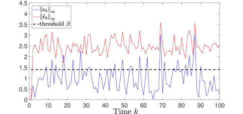
Figure 2: The triggering of event-based scheduler.

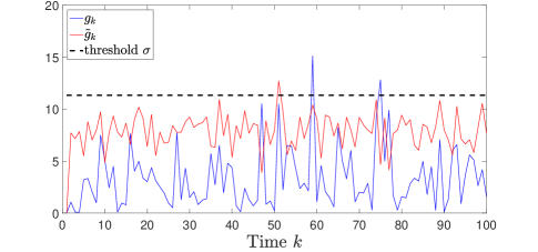
Figure 3: False data detection of $\chi^{2}$ detector.

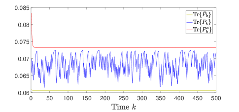
Figure 4: Remote estimation covariance for 3 cases.

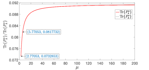
Figure 5: Steady state estimation covariance for different $\mu$.

6 Conclusion

In this paper, we proposed a novel deception attack strategy on event-based remote state estimator. The corresponding feasibility conditions were analyzed to ensure the attack can degrade the event-based scheduler performance while successfully bypassing the $\chi^{2}$ detector. Under the assumption that the event-based scheduler was triggered with probability $1$ after attack, we investigated the evolution of the remote estimation error covariance under the attack and analyzed the degradation of system performance. Furthermore, numerical simulations were presented to demonstrate the attack effectiveness.

References

• [1] Radha Poovendran, Krishna Sampigethaya, Sandeep KumarΒ S Gupta, Insup Lee, KΒ Venkatesh Prasad, David Corman, and JamesΒ L Paunicka. Special issue on cyber-physical systems. Proceedings of the IEEE, 100(1):1–12, 2012.
• [2] Heng Zhang, Peng Cheng, Ling Shi, and Jiming Chen. Optimal denial-of-service attack scheduling with energy constraint. IEEE Transactions on Automatic Control, 60(11):3023–3028, 2015.
• [3] Yao Liu, Peng Ning, and MichaelΒ K Reiter. False data injection attacks against state estimation in electric power grids. ACM Transactions on Information and System Security, 14(1):1–33, 2011.
• [4] Andre Teixeira, KinΒ Cheong Sou, Henrik Sandberg, and KarlΒ Henrik Johansson. Secure control systems: A quantitative risk management approach. IEEE Control Systems Magazine, 35(1):24–45, 2015.
• [5] Yilin Mo and Bruno Sinopoli. Secure control against replay attacks. In Proceedings of the 47th annual Allerton conference on Communication, Control, and Computing, pages 911–918, Monticello, IL, USA, October 2009.
• [6] Yilin Mo, Rohan Chabukswar, and Bruno Sinopoli. Detecting integrity attacks on scada systems. IEEE Transactions on Control Systems Technology, 22(4):1396–1407, 2013.
• [7] Ziyang Guo, Dawei Shi, KarlΒ Henrik Johansson, and Ling Shi. Optimal linear cyber-attack on remote state estimation. IEEE Transactions on Control of Network Systems, 4(1):4–13, 2016.
• [8] Zhong-Hua Pang, Guo-Ping Liu, Donghua Zhou, Fangyuan Hou, and Dehui Sun. Two-channel false data injection attacks against output tracking control of networked systems. IEEE Transactions on Industrial Electronics, 63(5):3242–3251, 2016.
• [9] Yuqing Ni, Ziyang Guo, Yilin Mo, and Ling Shi. On the performance analysis of reset attack in cyber-physical systems. IEEE Transactions on Automatic Control, 65(1):419–425, 2019.
• [10] Liang Hu, Zidong Wang, Qing-Long Han, and Xiaohui Liu. State estimation under false data injection attacks: Security analysis and system protection. Automatica, 87:176–183, 2018.
• [11] Dawei Shi, Tongwen Chen, and Ling Shi. Event-triggered maximum likelihood state estimation. Automatica, 50(1):247–254, 2014.
• [12] Junfeng Wu, Qing-Shan Jia, KarlΒ Henrik Johansson, and Ling Shi. Event-based sensor data scheduling: Trade-off between communication rate and estimation quality. IEEE Transactions on Automatic Control, 58(4):1041–1046, 2012.
• [13] AHΒ Nuttall. Some integrals involving the $Q_{M}$ function. IEEE Transactions on Information Theory, 21(1):95–96, 1975.
• [14] Annamalai Annamalai, Chintha Tellambura, and John Matyjas. A new twist on the generalized Marcum $Q$-function $Q_{M}(a,b)$ with fractional-order ${M}$ and its applications. In Proceedings of the 6th IEEE Conference on Consumer Communications and Networking Conference, pages 1–5, Las Vegas, NV, USA, February 2009.
• [15] Yin Sun and ÁrpΓ‘d Baricz. Inequalities for the generalized Marcum $Q$-function. Applied Mathematics and Computation, 203(1):134–141, 2008.
• [16] JIΒ Marcum. Table of $Q$-functions, U.S. air force project RAND res. memo. M-339, ASTIA document AD 1165451. Technical report, Rand Corp., Santa Monica, CA, USA, 1950.
• [17] Yin Sun, ÁrpΓ‘d Baricz, and Shidong Zhou. On the monotonicity, log-concavity, and tight bounds of the generalized marcum and nuttall $Q$-functions. IEEE Transactions on Information Theory, 56(3):1166–1186, 2010.
• [18] Rong Li and PooiΒ Yuen Kam. Computing and bounding the generalized marcum ${Q}$-function via a geometric approach. In Proceedings of the IEEE International Symposium on Information Theory, pages 1090–1094, Seattle, WA, USA, July 2006.
• [19] Ziyang Guo, Dawei Shi, KarlΒ Henrik Johansson, and Ling Shi. Worst-case stealthy innovation-based linear attack on remote state estimation. Automatica, 89:117–124, 2018.