Physics informed neural networks for continuum micromechanics

Abstract

Recently, physics informed neural networks have successfully been applied to a broad variety of problems in applied mathematics and engineering. The principle idea is the usage of a neural network as a global ansatz function for partial differential equations. Due to the global approximation, physics informed neural networks have difficulties in displaying localized effects and strong nonlinear solution fields by optimization. In this work we consider nonlinear stress and displacement fields invoked by material inhomogeneities with sharp phase interfaces. This constitutes a challenging problem for a method relying on a global ansatz. To overcome convergence issues, adaptive training strategies and domain decomposition are studied. It is shown, that the domain decomposition approach is capable to accurately resolve nonlinear stress, displacement and energy fields in heterogeneous microstructures obtained from real-world $\mu$CT-scans.

spacing=nonfrench [label1] organization=Institute for Computational Modeling in Civil Engineering, Technical University of Braunschweig, addressline=Pockelsstr. 3, city=Braunschweig, postcode=38106, country=Germany

[label3] organization=Chair of Engineering Mechanics, University of Paderborn, addressline=Warburger Str. 100, city=Paderborn, postcode=33098, country=Germany

1 Introduction

Problems in continuum mechanics arise in many areas of engineering, like civil-, mechanical- and aerospace engineering. The development of hybrid materials such as fiber reinforced plastics offers great potential for lightweight design due to their high strength to density ratio, compared to classic engineering materials. Unfortunately, these materials also raise the computational effort of meshing and simulation, as their overall macroscopic behavior is defined by their underlying heterogeneous microstructure. In order to resolve tensor fields of interest, like displacement, stress and strain fields, numerical methods have to be used in absence of analytical solutions. The most widely used numerical method, especially in computational mechanics, is the finite element method (FEM). Despite its broad range of applications and the successes therein, open problems remain. Among these, multi-scale problems, uncertainty quantification and inverse problems impose challenges to FEM. The reader is referred to [1] for a recent review.

An alternative to conventional numerical methods are artificial neural networks (ANN). ANNs are able to solve a wide range of problems, such as computer vision, speech recognition and autonomous driving [2]. In the scientific context, ANNs gain more and more popularity. They were successfully applied in fields like quantum mechanics [3], bioinformatics [4], medicine [5] and applied mathematics [6]. Recently, several investigations were made in the field of continuum mechanics [7]. Applications reach from fluid mechanics [8] over fracture mechanics [9] to micromechanics in the context of uncertainty quantification of effective properties [10].

While traditional ANN approaches need large datasets for training, the discovery of physics informed neural networks (PINNs) provides a framework for small data regimes. PINNs are introduced in [11] and have been reinvented using automatic differentiation and application to time-dependent problems in [12]. Here, the amount of data needed to solve scientific problems can even be reduced to initial and boundary conditions by solving the underlying governing equations, which are often described by partial differential equations (PDEs) [13]. PINNs therefore present an alternative to established numerical methods like FEM. They were successfully applied to bioinformatics [14], power systems [15] and chemistry [16], among other fields.

Like in the case of standard ANNs, several contributions of PINNs to continuum mechanics were published. Among these, fluid mechanics were considered in the context of flow visualization [17], multi-physics additive manufacturing simulations [18] and free surface flows [19], as well as for numerous other applications, see [20] for a review. In solid mechanics, PINNs were applied to solve problems in curing [21], material identification [22], heat transfer [23], forward problems in plate theory [24], plasticity [25], elastodynamics [26] and surrogate modeling [25]. Elastostatics were tackled using energy based methods for linear elasticity [27] and hyperelasticity [28]. Energy based error bounds can be found in [29]. The reconstruction of material distributions from given strain fields was the topic of [30].

While the effectiveness of the PINN approach in applications to continuum mechanics in the context of homogeneous materials was shown in the literature, to the best of the authors knowledge no attempts were made to resolve displacement and stress fields resulting from inhomogeneous material distributions using PINNs directly without the need of additional data. In the context of micromechanics, the knowledge of the exact micro stress field is crucial for full field homogenization. Unfortunately, several problems arise in this context, such as jumps in material parameters, highly nonlinear solution fields and convergence. The convergence to an optimal solution in the context of PINN was proved for linear PDEs [31] but the performance of these techniques in inhomogeneous cases remains open. In this context, classical techniques known from standard numerical methods, like h- and p-refinement (capacity of the ANN), are investigated for PINNs. To gain confidence in the ability of PINNs to capture the underlying physics of inhomogeneous micromechanics, the present study therefore aims towards the following key contributions:

• PINN elastostatics of inhomogeneous materials: A PINN for calculating displacement, stress and energy fields for arbitrary microstructural unit cells with arbitrary material parameters is proposed. The topology choices, loss calculation, boundary conditions and scaling methods are discussed in detail.

• Adaptivity and domain decomposition: To improve convergence, an adaptive collocation point sampling algorithm (h-refinement) as well as a domain decomposition technique (p-refinement) are discussed.

• $\bm{\mu}$CT-scan of wood-plastic composite: The proposed method’s performance is investigated on a real-world $\mu$CT-scan of a wood-plastic composite. To resolve the microstructure, a material network is introduced to render a smooth extension of voxelized image data. It is shown, that the PINN approach is able to accurately solve the micromechanical boundary value problem (BVP) of inhomogeneous elastostatics.

The proposed PINN solves the strong form of the underlying BVP directly, thus it allows to work with voxelized image data in a straightforward manner. Moreover, the formulation is flexible, making it easy to add additional physical or experimental information into the solution process. This opens up the application of this method in uncertainty quantification and inverse problems, such as the identification of uncertain material parameters. This is in contrast to the Deep Energy Method (DEM) [27, 32], where the principal of stationary elastic potential or energy approach was used for homogeneous problems in computational mechanics. DEM relies on integration of the energy formulation and uses a regular grid. Also, it is not well-suited for inverse heterogeneous problems, as the energy, used as optimization variable, is a global measure. Therefore, two local stress fields can lead to the same non-unique global energy value. Furthermore, the trivial solution always leads to a minimum of the energy, thus prohibiting the identification of parameters.

The remainder of this paper is structured as follows. In Section 2, the governing equations of linear elastic micromechanics are reviewed. Section 3 summarizes the basic equations and concepts of ANN and PINN. In Section 4, aspects of PINN discretization in the context of linear elastic micromechanics, including discussions about network topology, loss function calculation, boundary condition handling and scaling methods. The section closes with two numerical examples. Then, advanced techniques such as adaptivity and domain decomposition are developed in Section 5. A convergence study, comparing all proposed methods, is conducted. The best performing techniques are then used to calculate micro displacement and micro stress fields of a real-world $\mu$CT-scan of a wood-plastic composite in Section 6. To reach a smooth extension of the discrete voxelized image resulting from $\mu$CT-scans, a material network is proposed. The paper closes with a summary and an outlook in Section 7.

2 Governing equations of linear elastic micromechanics

In this section, a short overview of the governing equations of micromechanics, following [33] is given. The PDEs considered in this work arise in the context of elastostatics, assuming linear elastic material behaviour. To this end, the domain of interest $\Omega$ is chosen to be a symmetric and zero-centered square unit cell, such that

$$\Omega=\left\{\bm{x}=\left\{x^{d}\right\}\in\mathbb{R}^{d}\;\bigg{|}\;\frac{-L}{2}\leq x^{d}\leq\frac{L}{2}\right\}.$$ ((1))

Here, $\bm{x}$ are points in the domain $\Omega$ and $L$ denotes the edge length of the unit cell $\Omega$. The boundary of the domain $\Omega$ is denoted by

$$\partial\Omega=\partial\Omega_{\bar{u}}\cup\partial\Omega_{\bar{t}},\quad\partial\Omega_{\bar{u}}\cap\partial\Omega_{\bar{t}}=\emptyset,$$ ((2))

where $\Omega_{\bar{u}}$ are sections subject to Dirichlet boundary conditions

$$\bm{u}(\bm{x})=\bar{\bm{u}}(\bm{x}),\quad\bm{x}\in\partial\Omega,$$ ((3))

where $\bm{u}(\bm{x})$ is a displacement vector field and $\bar{\bm{u}}(\bm{x})$ represent prescribed displacements. Furthermore, $\partial\Omega_{\bar{t}}$ is subject to Neumann boundary conditions

$$\bm{t}(\bm{x})={\bm{\sigma}}(\bm{x})\cdot\bm{n}(\bm{x})=\bar{\bm{t}}(\bm{x})=\bar{\bm{\sigma}}(\bm{x})\cdot\bm{n}(\bm{x}),\quad\bm{x}\in\partial\Omega,$$ ((4))

with traction $\bm{t}(\bm{x})$, stress tensor field ${\bm{\sigma}}(\bm{x})$, normal vector $\bm{n}(\bm{x})$ and prescribed traction $\bar{\bm{t}}(\bm{x})$. The governing equations include the balance law of linear momentum

$$\nabla\cdot\bm{\sigma}(\bm{x})=0,\quad\bm{x}\in\Omega,$$ ((5))

excluding body forces and dynamic terms. Symmetry of the stress tensor $\bm{\sigma}(\bm{x})$ guarantees the balance of angular momentum

$$\bm{\sigma}(\bm{x})=\bm{\sigma}^{T}(\bm{x}),\quad\bm{x}\in\Omega.$$ ((6))

The displacement vector field $\bm{u}(\bm{x})$ can be related to a strain tensor field $\bm{\varepsilon}(\bm{x})$ by the kinematic relation

$$\bm{\varepsilon}(\bm{x})=\frac{1}{2}\left(\nabla\bm{u}(\bm{x})+\nabla\bm{u}^{T}(\bm{x})\right),\quad\bm{x}\in\Omega.$$ ((7))

The stress tensor field ${\bm{\sigma}}(\bm{x})$ and the strain tensor field $\bm{\varepsilon}(\bm{x})$ are related by a constitutive relation or material law. In this work, linear elasticity is investigated, in which the material law takes the form

$$\bm{\sigma}(\bm{x})=\lambda(\bm{x})\operatorname{tr}({\bm{\varepsilon}}(\bm{x}))\mathbb{I}+2\mu(\bm{x})\bm{\varepsilon}(\bm{x}),\quad\bm{x}\in\Omega,$$ ((8))

where $\lambda(\bm{x})$ and $\mu(\bm{x})$ are scalar fields, representing Lamé’s first and second constant, respectively and $\mathbb{I}$ denotes the second order identity tensor. Finally, the balance of internal work

$$W_{int}=\displaystyle\frac{1}{2}\displaystyle\int_{\Omega}\bm{\varepsilon}(\bm{x}):\bm{\sigma}(\bm{x})\mathrm{d\Omega},$$ ((9))

and external work

$$W_{ext}=\displaystyle\int_{\partial\Omega}\bar{\bm{t}}(\bm{x})\cdot\bm{u}(\bm{x})\mathrm{d\partial\Omega}=\displaystyle\int_{\partial\Omega}\bar{\bm{\sigma}}(\bm{x})\cdot\bm{n}(\bm{x})\cdot\bm{u}(\bm{x})\mathrm{d\partial\Omega},$$ ((10))

can be expressed by $W_{int}=W_{ext}$ and

$$\frac{1}{2}\displaystyle\int_{\Omega}\bm{\varepsilon}(\bm{x}):\bm{\sigma}(\bm{x})\mathrm{d\Omega}=\displaystyle\int_{\partial\Omega}\bar{\bm{t}}(\bm{x})\cdot\bm{u}(\bm{x})\mathrm{d\partial\Omega}=\displaystyle\int_{\partial\Omega}\bar{\bm{\sigma}}(\bm{x})\cdot\bm{n}(\bm{x})\cdot\bm{u}(\bm{x})\mathrm{d\partial\Omega}.$$ ((11))

The primary variable of the micromechanical balance of linear momentum in Eq. (5) is the displacement vector $\bm{u}(\bm{x})$ introduced in Eq. (3). By inserting the material law in Eq. (8) as well as the kinematic relation from Eq. (7) into the balance law Eq. (5), one obtains the Navier-Cauchy equations for homogeneous materials

$$\mu\Delta\bm{u}(\bm{x})+(\lambda+\mu)\nabla(\nabla\cdot\bm{u}(\bm{x}))=0.$$ ((12))

For inhomogeneous materials, inserting the material law Eq. (12) and the kinematic relation Eq. (7) into the balance law Eq. (5) leads to

$$\nabla\cdot\left(\lambda(\bm{x})\operatorname{tr}\left(\frac{1}{2}\left(\nabla\bm{u}(\bm{x})+\nabla\bm{u}^{T}(\bm{x})\right)\right)\mathbb{I}+\mu(\bm{x})(\nabla\bm{u}(\bm{x})+\nabla\bm{u}^{T}(\bm{x}))\right)=0,$$ ((13))

due to chained derivatives.

3 Artificial neural networks and physics informed neural networks

Whereas traditional numerical methods like FEM are often concerned with local ansatz functions, PINNs use global ansatz functions to find a global solution for the given BVP. This results in a complex optimization process, solved during training of an ANN. In the following, ANNs are concisely introduced in Section 3.1 and the theory of PINNs is explained in Section 3.2. In Section 4, PINNs are then used to discretize and solve BVPs appearing in Section 2.

3.1 Artificial neural networks

This section introduces the notation used in the context of ANNs. The reader familiar with this topic may proceed directly with Section 3.2.

An ANN is a parametrized, nonlinear function composition. By the universal function approximation theorem [34], arbitrary Borel measurable functions can be approximated by an ANN. There are several different formulations for ANN, which can be found in standard references such as [35, 36, 37, 38, 39]. In this paper, densely connected feed forward neural networks are used, which will be denoted by $\mathcal{N}$. For the reminder of this contribution the abbreviation ANN is understood as referring to such type of neural network. An ANN $\mathcal{N}$ is a function from an input space $\mathbb{R}^{d_{x}}$ to an output space $\mathbb{R}^{d_{y}}$, defined by a composition of nonlinear functions, such that

$$\mathcal{N}:\mathbb{R}^{d_{x}} \to\mathbb{R}^{d_{y}}$$

$$\bm{x} \mapsto\mathcal{N}(\bm{x})=\bm{h}^{(l)}\circ\ldots\circ\bm{h}^{(0)}=\bm{y},\quad l=1,\ldots,n_{L}.$$ ((14))

Here, $\bm{x}$ denotes an input vector of dimension $d_{x}$ and $\bm{y}$ an output vector of dimension $d_{y}$. The nonlinear functions $\bm{h}^{(l)}$ are called layers and define a $l$-fold composition, mapping input vectors $\bm{x}$ to output vectors $\bm{y}$. Consequently, the first layer $\bm{h}^{(0)}$ is defined as the input layer and the last layer $\bm{h}^{(n_{L})}$ as the output layer, such that

$$\bm{h}^{(0)}=\bm{x}\in\mathbb{R}^{d_{x}},\qquad\bm{h}^{(n_{L})}=\bm{y}\in\mathbb{R}^{d_{y}}.$$ ((15))

The layers $\bm{h}^{(l)}$ between the input and output layer, called hidden layers, are defined as

$$\bm{h}^{(l)}=\left\{h_{\eta}^{(l)},\;\eta=1,\ldots,n_{u}\right\},\qquad h_{\eta}^{(l)}=\phi^{(l)}\left(\bm{W}^{(l)}_{\eta}\bm{h}^{(l-1)}\right)=\phi^{(l)}\left({z}_{\eta}^{(l)}\right),$$ ((16))

where $h_{\eta}^{(l)}$ is the $\eta$-th neural unit of the $l$-th layer $\bm{h}^{(l)}$ and $n_{u}$ is the total number of neural units per layer, which in this work is constant over all layers. $\phi^{(l)}$ is a nonlinear activation function from $\mathbb{R}\to\mathbb{R}$, which in this work is defined by means of the so called Swish function [40] as

$$\phi^{(l)}\left({z}_{\eta}^{(l)}\right)=\operatorname{swish}\left({z}_{\eta}^{(l)}\right)=\displaystyle\frac{1}{1+e^{-\beta{z}_{\eta}^{(l)}}},\quad{z}_{\eta}^{(l)},\beta\in\mathbb{R}$$ ((17))

with

$$\phi^{(n_{L})}\left({z}_{\eta}^{(n_{L})}\right)=\operatorname{id}\left({z}_{\eta}^{(n_{L})}\right).$$ ((18))

Here, ${z}_{\eta}^{(l)}$ denotes the scalar valued product of the weight vector $\bm{W}_{\eta}^{(l)}$ of the $\eta$-th neural unit in the $l$-th layer $\bm{h}^{(l)}$ and the output of the preceding layer $\bm{h}^{(l-1)}$ in Eq. (16). In our notation we absorb the bias term, occurring in the standard notation, as explained, e.g., in [37]. All weight vectors $\bm{W}_{\eta}^{(l)}$ of all layers $\bm{h}^{(l)}$ can be gathered in a single expression, such that

$$\bm{\theta}=\left\{\bm{W}_{\eta}^{(l)}\right\},$$ ((19))

where $\bm{\theta}$ inherits all parameters of the ANN $\mathcal{N}(\bm{x})$ from Eq. (14). Consequently, the notation $\mathcal{N}(\bm{x};\bm{\theta})$ emphasises the dependency of the outcome of an ANN on the input on the one hand and the current realization of the weights on the other hand. A graphical representation of an ANN is shown in Figure 1, where the specific combination of layers $\bm{h}^{(l)}$ and neural units $h_{\eta}^{(l)}$ from Eq. (16) and activation functions $\phi^{(l)}$ from Eq. (17) is called topology of the ANN $\mathcal{N}(\bm{x};\bm{\theta})$.

Figure 1: Feed forward neural network topology of an ANN $\mathcal{N}(\bm{x};\bm{\theta})$ as described in Eq. (14).

3.2 Physics informed neural networks

An ANN $\mathcal{N}(\bm{x};\bm{\theta})$, as described in Section 3.1, can be used to solve PDEs by means of an optimization problem. This approach is called PINNs [12]. In this work, stationary elliptic nonlinear PDEs are considered, despite the fact that PINNs are applicable in more general settings as well [13]. Following the notation from [41], consider a BVP over a domain $\Omega$ with boundary $\partial\Omega$ defined by

$$\bm{Lu}(\bm{x})=\bm{f}(\bm{x}),\bm{x}\in\Omega\subset\mathbb{R}^{n},\qquad\bm{Bu}(\bm{x})=\bm{g}(\bm{x}),\bm{x}\in\Gamma\subset\partial\Omega,$$ ((20))

where $\bm{L}$ denotes a differential operator, $\bm{u}(\bm{x})$ is a real multivariate function of a real multivariate variable $\bm{x}$ of dimension $d$, representing spatial points of a domain $\Omega$, and $\bm{f}(\bm{x})$ is a forcing term. Furthermore, $\bm{B}$ is a boundary operator with respective boundary data $\bm{g}(\bm{x})$, which is imposed on the corresponding part $\Gamma$ of the boundary. In PINNs, the ansatz for solving Eq. (20) is defined by means of an ANN in Eq. (14) as

$$\bm{u}(\bm{x})\approx\mathcal{N}(\bm{x};\bm{\theta}).$$ ((21))

Because an ANN $\mathcal{N}(\bm{x};\bm{\theta})$ can approximate arbitrary functions, it is capable of representing the solution of the BVP given appropriate parameters $\bm{\theta}$ from Eq. (19).

3.2.1 Optimization

The appropriate parameters $\bm{\theta}$ in Eq. (19) of the ANN $\mathcal{N}(\bm{x};\bm{\theta})$ from Eq. (14)) can be found by utilizing a collocation method. The domain $\Omega$ and the boundary part $\Gamma$ from Eq. (20) are discretized into sets of collocation points $\Omega_{d}$ and $\Gamma_{d}$, respectively, with $|\Omega_{d}|=n_{d}$ and $|\Gamma_{d}|=n_{b}$. Then, an optimization problem to find the optimal parameters $\bm{\theta}^{*}$, also called training, is defined as

$$\bm{\theta}^{*}=\underset{\bm{\theta}}{\operatorname*{arg\,min}}\;\mathcal{L}(\bm{x};\bm{\theta})=\underset{\bm{\theta}}{\operatorname*{arg\,min}}\;\left(\mathcal{L}_{r}(\bm{x};\bm{\theta})+\mathcal{L}_{b}(\bm{x};\bm{\theta})\right),$$ ((22))

with

$$\mathcal{L}_{r}(\bm{x};\bm{\theta})=\displaystyle\sum_{\bm{x}\in\Omega_{d}}\displaystyle\frac{1}{n_{d}}||\bm{L}\mathcal{N}(\bm{x};\bm{\theta})-\bm{f}(\bm{x})||_{2}^{2},$$ ((23))

and

$$\mathcal{L}_{b}(\bm{x};\bm{\theta})=\displaystyle\sum_{\bm{x}\in\Gamma_{d}}\displaystyle\frac{1}{n_{b}}||\bm{B}\mathcal{N}(\bm{x};\bm{\theta})-\bm{g}(\bm{x})||_{2}^{2},$$ ((24))

where $\bm{\theta}^{*}$ are the optimal weights and biases with respect to the objective function $\mathcal{L}(\bm{x};\bm{\theta})$. The expression $\mathcal{L}(\bm{x};\bm{\theta})$ in Eq. (22) is also called loss function and contains a residual term $\mathcal{L}_{r}(\bm{x};\bm{\theta})$ of the PDE in Eq. (23) as well as a term $\mathcal{L}_{b}(\bm{x};\bm{\theta})$ in Eq. (24), describing the discrepancy of the boundary conditions. The spatial derivatives in the loss function can be obtained by automatic differentiation of the ANN $\mathcal{N}(\bm{x};\bm{\theta})$ using open source frameworks like Tensorflow [42]. The automatic differentiation of Eq. (14) with respect to the spatial coordinates implies the chain rule.

3.2.2 Boundary conditions

The formulation of the optimization problem in Eq. (22) enforces the boundary conditions in Eq. (20) by means of a separate loss term $\mathcal{L}_{b}(\bm{x};\bm{\theta})$. This approach is called soft boundary conditions in PINN terminology [43]. The boundary conditions are fulfilled, if the loss term $\mathcal{L}_{b}(\bm{x};\bm{\theta})$ vanishes. On the other hand, so called hard boundary conditions include the boundary conditions in the formulation of the ANN in Eq. (14) a priori. Following the approach in [41], hard boundary conditions can be realized by letting the boundary operator $\bm{B}$ from Eq. (20) be the identity operator. Then, the ansatz is formulated as

$${\mathcal{N}}(\bm{x};\bm{\theta})=\bm{G}(\bm{x})+\bm{D}(\bm{x})\tilde{\mathcal{N}}(\bm{x};\bm{\theta}),$$ ((25))

where $\bm{G}(\bm{x})$ is a smooth extension of the boundary data $\bm{g}(\bm{x})$ in Eq. (20) and $\bm{D}(\bm{x})$ is a smooth distance function. $\tilde{\mathcal{N}}(\bm{x};\bm{\theta})$ denotes an ANN without boundary condition restrictions. If the distance function $\bm{D}(\bm{x})$ vanishes, the point $\bm{x}$ lies on the boundary and the output of the ANN is automatically neglected. The functions $\bm{G}(\bm{x})$ and $\bm{D}(\bm{x})$ can be given analytically or represented by ANNs. The advantage of hard boundary conditions over soft boundary conditions is the reduced complexity of the optimization problem in Eq. (22), which simplifies to

$$\bm{\theta}^{*}=\underset{\bm{\theta}}{\operatorname*{arg\,min}}\;\mathcal{L}(\bm{x};\bm{\theta})=\underset{\bm{\theta}}{\operatorname*{arg\,min}}\;\mathcal{L}_{r}(\bm{x};\bm{\theta}).$$ ((26))

The loss function consists only of the residual loss $\mathcal{L}_{r}(\bm{x};\bm{\theta})$ in Eq. (23) with respect to the PDE in Eq. (20).

4 Physics informed neural networks for linear elasticity

In this work, the linear elastostatic balance law of linear momentum presented in Eq. (5) is directly solved using its strong form.

To solve BVP in linear elasticity, a suitable topology for the ANN in Eq. (14) and consequently the PINN described in Section 3.2 has to be chosen. One possibility is to let the output layer $\bm{h}^{(n_{L})}$ of the ANN be the tuple of the displacement vector field components $\bm{u}(\bm{x})$ in Eq. (3), i.e. the primary variables, such that

$$\mathcal{N}(\bm{x};\bm{\theta})=\left\{\mathcal{N}_{u_{x}}(\bm{x};\bm{\theta}),\mathcal{N}_{u_{y}}(\bm{x};\bm{\theta})\right\}.$$ ((27))

Then, the ANN can be used to solve the inhomogeneous Navier-Cauchy equation in Eq. (13), such as e.g., in [32]. Unfortunately, several problems arise along utilization of such an approach. First, in Eq. (13) the derivatives of the material parameters $\lambda(\bm{x})$ and $\mu(\bm{x})$ are needed. For sharp material phase transitions, numerical problems can arise during optimization in Eq. (22) due to exploding gradients. Second, in Eq. (13) second derivatives of the displacement vector $\bm{u}(\bm{x})$ are needed. The computation of these introduces additional overhead during optimization. Third, the application of mixed boundary conditions renders more difficult, as e.g. free boundary stress conditions cannot be imposed in a straightforward fashion using hard boundary conditions described in Eq. (25).

Alternatively, let the ANN output include the displacements $\bm{u}(\bm{x})$ and the stresses $\bm{\sigma}(\bm{x})$, such that

$$\mathcal{N}(\bm{x};\bm{\theta})=\left\{\mathcal{N}_{u_{x}}(\bm{x};\bm{\theta}),\mathcal{N}_{u_{y}}(\bm{x};\bm{\theta}),\mathcal{N}_{\sigma_{xx}}(\bm{x};\bm{\theta}),\mathcal{N}_{\sigma_{yy}}(\bm{x};\bm{\theta}),\mathcal{N}_{\sigma_{xy}}(\bm{x};\bm{\theta})\right\}.$$ ((28))

In the two-dimensional setting this includes two displacement components $u_{x}(\bm{x})$, $u_{y}(\bm{x})$ and three stress components $\sigma_{xx}(\bm{x})$, $\sigma_{yy}(\bm{x})$, $\sigma_{xy}(\bm{x})$, as the symmetry of the stress tensor ensures balance of angular momentum Eq. (6). This approach allows the direct computation of the balance law Eq. (5) without the usage of second order derivatives. An illustration of the PINN is shown in Figure 2. Furthermore, this topology simplifies the applicability of hard boundary conditions as explained in Eq. (25). The detailed formulations of the function in Eq. (25) is case dependent and will be explained in the experimental section, see Section 4.3.

Figure 2: Topology of a PINN $\mathcal{N}(\bm{x};\bm{\theta})$ for linear elasticity.

4.1 Loss function and boundary conditions

Using hard boundary conditions, the loss function in Eq. (22) does only contain residual terms. In the two-dimensional setting, these include

$$\mathcal{L}_{PINN}(\bm{x};\bm{\theta}) =\mathcal{L}_{\nabla}^{x}(\bm{x};\bm{\theta})+\mathcal{L}_{\nabla}^{y}(\bm{x};\bm{\theta})$$ ((29))

$$+\mathcal{L}_{const}^{xx}(\bm{x};\bm{\theta})+\mathcal{L}_{const}^{yy}(\bm{x};\bm{\theta})+\mathcal{L}_{const}^{xy}(\bm{x};\bm{\theta})$$

$$+\mathcal{L}_{W}(\bm{x};\bm{\theta}),$$

with

$$\mathcal{L}_{\nabla}^{x}(\bm{x};\bm{\theta}) =\langle\partial_{x}\mathcal{N}_{\sigma_{xx}}+\partial_{y}\mathcal{N}_{\sigma_{xy}}\rangle,$$

$$\mathcal{L}_{\nabla}^{y}(\bm{x};\bm{\theta}) =\langle\partial_{x}\mathcal{N}_{\sigma_{xy}}+\partial_{y}\mathcal{N}_{\sigma_{yy}}\rangle,$$

$$\mathcal{L}_{const}^{xx}(\bm{x};\bm{\theta}) =\langle\lambda\left(\partial_{x}\mathcal{N}_{u_{x}}+\partial_{y}\mathcal{N}_{u_{y}}\right)+2\mu\partial_{x}\mathcal{N}_{u_{x}}-\mathcal{N}_{\sigma_{xx}}\rangle,$$

$$\mathcal{L}_{const}^{yy}(\bm{x};\bm{\theta}) =\langle\lambda\left(\partial_{x}\mathcal{N}_{u_{x}}+\partial_{y}\mathcal{N}_{u_{y}}\right)+2\mu\partial_{y}\mathcal{N}_{u_{y}}-\mathcal{N}_{\sigma_{yy}}\rangle,$$

$$\mathcal{L}_{const}^{xy}(\bm{x};\bm{\theta}) =\langle\mu\left(\partial_{y}\mathcal{N}_{u_{x}}+\partial_{x}\mathcal{N}_{u_{y}}\right)-\mathcal{N}_{\sigma_{xy}}\rangle,$$

$$\mathcal{L}_{W}(\bm{x};\bm{\theta}) =\bigg{|}\bigg{|}\displaystyle\sum_{\bm{x}\in\Omega_{d}}\displaystyle\frac{L^{2}}{2n_{d}}\mathcal{L}_{W}^{int}(\bm{x};\bm{\theta})-\displaystyle\sum_{\bm{x}\in\Gamma_{d}}\displaystyle\frac{1}{n_{b}}\mathcal{L}_{W}^{ext}(\bm{x};\bm{\theta})\bigg{|}\bigg{|}_{2}^{2}$$

$$\mathcal{L}_{W}^{int}(\bm{x};\bm{\theta}) =\mathcal{N}_{\sigma_{xx}}\partial_{x}\mathcal{N}_{u_{x}}+\mathcal{N}_{\sigma_{yy}}\partial_{y}\mathcal{N}_{u_{y}}+\mathcal{N}_{\sigma_{xy}}\left(\partial_{y}\mathcal{N}_{u_{x}}+\partial_{x}\mathcal{N}_{u_{y}}\right)$$

$$\mathcal{L}_{W}^{ext}(\bm{x};\bm{\theta}) =\mathcal{N}_{\sigma_{xx}}\mathcal{N}_{u_{x}}+\mathcal{N}_{\sigma_{xy}}\mathcal{N}_{u_{y}},$$

where

$$\mathcal{N}_{\bullet}=\mathcal{N}_{\bullet}(\bm{x};\bm{\theta}),\qquad\lambda=\lambda(\bm{x}),\qquad\mu=\mu(\bm{x})$$

$$\partial_{\star}\bullet=\frac{\partial\bullet}{\partial\star},\qquad\langle\bullet\rangle=\displaystyle\sum_{\bm{x}\in\Omega_{d}}\displaystyle\frac{1}{n_{d}}\bigg{|}\bigg{|}\bullet\bigg{|}\bigg{|}_{2}^{2}.$$

Here, $\mathcal{L}_{\nabla}^{x}(\bm{x};\bm{\theta})$ and $\mathcal{L}_{\nabla}^{y}(\bm{x};\bm{\theta})$ are the residuals of the balance law in Eq. (5), $\mathcal{L}_{const}^{xx}(\bm{x};\bm{\theta})$, $\mathcal{L}_{const}^{yy}(\bm{x};\bm{\theta})$, $\mathcal{L}_{const}^{xy}(\bm{x};\bm{\theta})$ include the constitutive relation in Eq. (8) and the kinematic relation in Eq. (7), whereas $\mathcal{L}_{W}(\bm{x};\bm{\theta})$ represents the work balance in Eq. (11). The work balance loss $\mathcal{L}_{W}(\bm{x};\bm{\theta})$ in Eq. (29) ensures global conservation, whereas the other terms represent local laws.

Remark: In several works, such as [44] and [45], a weight factor is added to the individual loss terms in Eq. (29). However, in this work no such factors are used, as numerical experiments carried out by the author did not show any improvement over equally weighted terms. An exception is the domain decomposition approach presented in Section 5.2, where a constant weight factor is used for the additional interface terms. This may be related to the usage of full BFGS optimization algorithms instead of L-BFGS and ADAM and the much simpler loss functions compared to other works, such as [44] and [45].

4.2 Loss scaling

The quantities of the governing equations in Section 2, namely the spatial location $\bm{x}$, the stress $\bm{\sigma}(\bm{x})$, the displacement $\bm{u}(\bm{x})$ as well as the material parameters $\lambda(\bm{x})$ and $\mu(\bm{x})$ have large differences in their respective absolute values. Whereas the displacement is typically in the range of $u_{\bullet}<<1$ mm, the material parameters lie in the order of $(\lambda,\mu)>>10^{3}$ MPa. These discrepancies lead to difficulties during optimization of the loss function $\mathcal{L}_{PINN}$ in Eq. (29). To overcome this problem, the values mentioned above are rescaled internally to lie in a common order, before calculating the loss terms. This also applies to boundary conditions. Every quantity is divided by a respective constant, such that

$$\hat{\bm{x}}=\frac{\bm{x}}{x_{c}},\;\hat{\bm{\sigma}}(\bm{x})=\frac{\bm{\sigma}(\bm{x})}{\sigma_{c}},\;\hat{\bm{u}}(\bm{x})=\frac{\bm{u}(\bm{x})}{u_{c}},\;\hat{\lambda}(\bm{x})=\frac{\lambda(\bm{x})}{\lambda_{c}},\;\hat{\mu}(\bm{x})=\frac{\mu(\bm{x})}{\mu_{c}}.$$ ((30))

The rescaled entities used for calculation, denoted by $\hat{\bullet}$, need to be scaled back again into its natural range during prediction, to yield quantitatively correct results. Typically, the scaling factors $\bullet_{c}$ are chosen to be the maximum value of the entity under consideration with respect to the domain $\Omega$ in Eq. (1). Note that the scaling only affects the weighting of the different loss terms, thus impacts sole the optimization dynamics, but not the dynamics of the PDE and the spatial derivatives involved. This is because we consider a linear PDE in Section 4. The obtained solution fields depend qualitatively on the microstructure, the material parameters’ phase contrast of the different materials involved and the specific kind of boundary condition in the BVP. Quantitatively the solution fields depend on the values of the single material parameters and the boundary condition applied. Once solved, the solution field can be scaled as needed. This parametrization enables generalization to different boundary condition values.

Remark: For the sake of simplicity, along this work the unscaled quantities were used throughout the text and formulae. The rescaling is only used internally during loss calculation. For large material contrasts, the proposed PINN method cannot converge without loss scaling.

4.3 Numerical experiments - PINN

In the following, the proposed method described in Section 4 is investigated by several numerical experiments. First, in Section 4.3.1, a homogeneous case is considered. Second, in Section 4.3.2, the same experimental setup but with a single inclusion added to the domain is carried out. This turns the BVP into an inhomogeneous problem, to compare the effect of heterogeneity on the proposed method. If not stated otherwise, all experiments were carried out on a Nvidia Quadro M5000M GPU using single-precision floating-point format and TensorFlow 2 [42].

4.3.1 Homogeneous plate - PINN

The first example considers a two-dimensional square domain $\Omega$, with dimension $d=2$, from Eq. (1) with a homogeneous material distribution shown in Figure 3(a). The domain is subject to Neumann boundary conditions for static loading $\bar{\sigma}$ and stress-free boundaries from Eq. (4). Dirichlet displacement boundary conditions from Eq. (3) ensure that no free-body movements occur. For this example, a PINN as described in Section 4, with $n_{L}=4$ and $n_{u}=64$, as defined in Eq. (14) and Eq. (15), is used. The capacity increase of the ANN in terms of number of parameters $\bm{\theta}$ can be seen as a form of p-refinement. The topology presented led to the best results in preceding experiments, which are not shown in this work. The inputs $\bm{h}^{(0)}$ are the spatial coordinates $\bm{h}^{(0)}=\bm{x}$ of the domain $\Omega$ from Eq. (1) with length $L=2$ mm, such that the domain is a zero centered square between $-1$ and $1$. A traction $\bar{\sigma}=0.025$ MPa is applied perpendicular to the boundary, which results in small strains in accordance to the linear elastic theory.

Remark: In FEM, the zero stress boundary conditions on free boundaries $\partial\Omega$ are fulfilled automatically due to the weak form used in the formulation. In the proposed PINN from Section 4, the strong form of the BVP is used. Therefore it is necessary to explicitly enforce the zero stress boundary conditions as seen in Figure 3.

The hard boundary conditions from Eq. (25) are enforced in consistency with Figure 3(b), such that

$${\mathcal{N}}_{u_{x}}(\bm{x};\bm{\theta}) =0+(-1-x)\tilde{\mathcal{N}}_{u_{x}}(\bm{x};\bm{\theta}),$$ ((31))

$${\mathcal{N}}_{u_{y}}(\bm{x};\bm{\theta}) =0+(-1-y)\tilde{\mathcal{N}}_{u_{y}}(\bm{x};\bm{\theta}),$$

$${\mathcal{N}}_{\sigma_{xx}}(\bm{x};\bm{\theta}) =\bar{\sigma}+(1-x)\tilde{\mathcal{N}}_{\sigma_{xx}}(\bm{x};\bm{\theta}),$$

$${\mathcal{N}}_{\sigma_{yy}}(\bm{x};\bm{\theta}) =0+(1-y)\tilde{\mathcal{N}}_{\sigma_{yy}}(\bm{x};\bm{\theta}),$$

$${\mathcal{N}}_{\sigma_{xy}}(\bm{x};\bm{\theta}) =0+\left((1-x)^{2}(1-y)^{2}\right)\tilde{\mathcal{N}}_{\sigma_{xy}}(\bm{x};\bm{\theta}),$$

The material parameters $\lambda(\bm{x})$ and $\mu(\bm{x})$ in the constitutive relation Eq. (8) are calculated from Young’s modulus $E=1\times 10^{4}$ MPa and Poisson’s ratio $\nu=0.4$. The collocation points described in Section 3.2.1 are chosen on a regular grid $\Omega_{d}$, whereas the number of collocation points is $n_{d}=128^{2}$. For the optimization problem in Section 3.2.1, the loss function in Eq. (29) is minimized by the BFGS algorithm [46], which terminated after 138 iterations due to gradient size. The prediction is carried out on a regular grid of $n_{d}=128^{2}$ collocation points.

The resulting components of the stress tensor field $\bm{\sigma}(\bm{x})$ and displacement vector field $\bm{u}(\bm{x})$ as well as the point-wise internal work $W_{int}(\bm{x})$ are shown in Figure 4. Several error measures are provided, namely the sum of the absolute residuals $\mathcal{R}$ as well as the single residuals for the balance law $\mathcal{R}_{\nabla}^{\bullet}=\{\mathcal{R}_{\nabla}^{x},\mathcal{R}_{\nabla}^{y}\}$ and the constitutive law $\mathcal{R}_{const}^{\bullet}=\{\mathcal{R}_{const}^{xx},\mathcal{R}_{const}^{yy},\mathcal{R}_{const}^{xy}\}$. They are defined as the component wise residuals of the balance law in Eq. (5) for $\mathcal{R}_{\nabla}^{\bullet}$ and the constitutive relation in Eq. (8) for $\mathcal{R}_{const}^{\bullet}$, respectively. $\mathcal{R}$ is defined as the sum of the absolute values of $\mathcal{R}_{\nabla}^{\bullet}$ and $\mathcal{R}_{const}^{\bullet}$. These residuals are obtained for the scaled units, as described in Section 4.2. Therefore, they are normalized error measures.

Remark: The contour plots for the stresses $\bm{\sigma}(\bm{x})$ and the point-wise internal work $W_{int}(\bm{x})$ as shown in Figure 4 show non-homogeneous solution fields. These, however, deviate only marginally from the correct homogeneous solution, as may be recognized from the color bar ranges.

It can be observed, that the PINN achieves low residual errors along the governing equations. Additionally, the L2-norm of the work balance loss from Eq. (29) is $||\mathcal{L}_{W}||:=\sqrt{\mathcal{L}_{W}}=2.84221187\times 10^{-6}$, indicating conservation of energy.

(a) Homogeneous

(b) Inhomogeneous

Figure 3: Rectangular domain $\Omega$ from Eq. (1) with length $L=2$ mm under uniaxial loading x-direction. Plane strain is assumed. The boundary conditions of (a) also apply to (b).

Figure 4: Homogeneous plate - PINN: The resulting components of the stress tensor field $\bm{\sigma}(\bm{x})$ and displacement vector field $\bm{u}(\bm{x})$ as well as the point wise internal work $W_{int}$ for the homogeneous plate from Section 4.3.1 in the top rows. In the bottom rows the absolute sum of the residuals $\mathcal{R}$ as well as the single residuals for the balance law $\mathcal{R}_{\nabla}^{\bullet}$ and the constitutive law $\mathcal{R}_{const}^{\bullet}$, as described in Section 4.3.2, are shown. The L2-norm of the work balance loss from Eq. (29) is $||{\mathcal{L}_{W}}||=2.84221187\times 10^{-6}$.

4.3.2 Single inclusion - PINN

The second example considers the same two-dimensional square domain $\Omega$ from Section 4.3.2 with inhomogeneous material distribution as depicted in Figure 3b. The domain contains a single circular inclusion and a surrounding matrix phase, whereas the material parameters for both phases are distinct. For inhomogeneous microstructures $\Omega$ from Eq. (1), the distribution of the material parameters $\lambda(\bm{x})$ and $\mu(\bm{x})$ in Eq. (8) is usually non-trivial. To obtain these scalar fields, $\mu$CT-scans are carried out in practice. These render a voxelized, discrete distribution of different material densities, from which material phases can be identified. Due to the discreteness, the transition between different phases are non-smooth. In the context of PINNs, the optimization problem in Section 3.2.1 becomes less involved for smoother and more homogeneous problems. To this end, the distribution of the material parameters $\lambda(\bm{x})$ and $\mu(\bm{x})$ in Eq. (8) is approximated by smooth functions. In the case of a square domain with a single inclusion, as seen in Figure 3b, the following equation is a smooth approximation of the material jump

$$\lambda(\bm{x}=\{x_{1},x_{2}\})=c_{1}\left(c_{2}+\operatorname{tanh}\left(\frac{0.4-\sqrt{x_{1}^{2}+x_{2}^{2}}}{\delta}\right)\right)+c_{3},$$ ((32))

where $c_{1}$, $c_{2}$ and $c_{3}$ are constants manipulating the shape and value of the inclusion and $\delta$ defines the steepness of the material phase transition.

The domain is subject to Neumann traction boundary conditions for static loading $\bar{\sigma}$ and stress-free boundaries from Eq. (4). Dirichlet displacement boundary conditions from Eq. (3) ensure that no free-body movements occur. For this example, a PINN as described in Section 4, with $n_{L}=4$ and $n_{u}=64$, as defined in Eq. (14) and Eq. (15), is used. The inputs $\bm{h}^{(0)}$ are the spatial coordinates $\bm{h}^{(0)}=\bm{x}$ of the domain $\Omega$ from Eq. (1) with length $L=2$, such that the domain is a zero centered square between $-1$ and $1$. The Neumann boundary condition from Eq. (4) is chosen as $\bar{\sigma}=0.025$ MPa and acts perpendicular to the boundary. The material parameters $\lambda(\bm{x})$ and $\mu(\bm{x})$ in the constitutive relation Eq. (8) are calculated from Young’s modulus $E=1\times 10^{4}$ MPa and Poisson’s ratio $\nu=0.4$ for the inclusion phase and $E=1.5\times 10^{3}$ MPa and $\nu=0.4$ for the matrix phase. The collocation points are chosen on a regular grid, whereas the number of collocation points is $n_{d}=128^{2}$. For the optimization problem in Section 3.2.1, the loss function in Eq. (29) is minimized by the BFGS algorithm [46]. The optimizer stopped after around $5\times 10^{3}$ iterations due to small gradient updates. The prediction is carried out on a regular grid of $n_{d}=128^{2}$ collocation points.

The resulting components of the stress tensor field $\bm{\sigma}(\bm{x})$ and displacement vector field $\bm{u}(\bm{x})$ as well as the point wise internal work $W_{int}(\bm{x})$ are shown in Figure 5. The same error measures as in the previous section are provided, namely the absolute sum of the residuals $\mathcal{R}$ as well as the single residuals for the balance law $\mathcal{R}_{\nabla}^{\bullet}=\{\mathcal{R}_{\nabla}^{x},\mathcal{R}_{\nabla}^{y}\}$ and the constitutive law $\mathcal{R}_{const}^{\bullet}=\{\mathcal{R}_{const}^{xx},\mathcal{R}_{const}^{yy},\mathcal{R}_{const}^{xy}\}$, which are defined in Section 4.3.2. It becomes clear, that the proposed method captures the inhomogeneity in the material parameters. The L2-norm of the work balance loss from Eq. (29) is $||{\mathcal{L}_{W}}||=6.93413196\times 10^{-3}$ and the mean residual is $\mathbb{E}(\mathcal{R})=4.1985224\times 10^{-4}$. The highest errors can be found at the material interfaces. Here, the maximum residual is $max(\mathcal{R})=1.782237\times 10^{-2}$. The minimum residual is $min(\mathcal{R})=1.6041845\times 10^{-4}$.

The PINN is able to qualitatively capture a global solution for the given BVP. Nevertheless, the phase transition remains problematic due to the sudden jump in the material parameters $\lambda(\bm{x})$ and $\mu(\bm{x})$ from Eq. (8). Therefore, in Section 5, two techniques are studied with the goal to counter this problem.

Figure 5: Single inclusion - PINN: The resulting components of the stress tensor field $\bm{\sigma}(\bm{x})$ and displacement vector field $\bm{u}(\bm{x})$ as well as the point wise internal work $W_{int}$ for the inhomogeneous plate from Section 4.3.2 in the top rows. In the bottom rows the absolute sum of the residuals $\mathcal{R}$ as well as the single residuals for the balance law $\mathcal{R}_{\nabla}^{\bullet}$ and the constitutive law $\mathcal{R}_{const}^{\bullet}$, as described in Section 4.3.1, are shown. The L2-norm of the work balance loss from Eq. (29) is $||\mathcal{L}_{W}||=4.1985224\times 10^{-4}$. Maximum number of BFGS iterations: $1\times 10^{4}$.

5 Adaptivity and domain decomposition

To reduce the error at the phase transitions, two techniques are studied in the upcoming sections. First, an adaptive algorithm for sampling the collocation points is proposed in Section 5.1. Second, a domain decomposition algorithm to use multiple ANNs on smaller sub-problems is investigated in Section 5.2. These are compared to the standard PINN approach in Section 5.3.

5.1 Adaptive collocation points

To overcome the high errors at the phase transitions reported in Section 4.3.2, an adaptive discretization scheme is proposed. The adaptive scheme is motivated by FEM h-refinement, where a local mesh refinement at points of interest leads to higher precision in stress flows. The difference to PINNs is once again, that FEM uses local ansatz functions, whereas PINNs are global ansatz functions. The goal is, that by training the PINN on collocation points with high errors, a global solution representing also localized nonlinearities of the stress and displacement distributions is found during optimization of the problem described in Section 3.2.1. In the following, the proposed adaptive algorithm is described.

A related but different approach can be found in [47]. First, a fine regular grid is chosen and the training is carried out as described in Section 4.3.2. This can be seen as a pre-training of the PINN. Then, for a user defined number of iterations, an adaptive scheme is used as follows. A set of collocation points $\Omega_{d}$ is formed by two subsets, one coarse regular grid $\Omega_{d}^{reg}$ and one adaptive set $\Omega_{d}^{rand}$. The set of regular grid points $\Omega_{d}^{reg}$ is defined as the Cartesian product

$$\Omega_{d}^{reg}=\left\{\bm{x}_{i}\in\left[-\frac{L}{2},\frac{L}{2}\right]\times\left[-\frac{L}{2},\frac{L}{2}\right],\;i=1,...,n_{reg}\right\}$$ ((33))

whereas the random points are chosen randomly from a uniform distribution

$$\Omega_{d}^{rand}=\left\{\bm{x}_{i}\sim\bm{\mathcal{U}}\left(-\frac{L}{2},\frac{L}{2}\right),\;i=1,...,n_{rand}\right\}$$ ((34))

Then the loss from Eq. (29) is calculated for the random points, with the work balance term neglected, as it is a global, not point-wise loss due to the appearance of the external work from Eq. (11). The loss is defined as

$$\mathcal{L}_{PINN}^{\sim W}(\bm{x};\bm{\theta})=\mathcal{L}_{PINN}(\bm{x};\bm{\theta})-\mathcal{L}_{W}(\bm{x};\bm{\theta}).$$ ((35))

The set of adaptive points $\Omega_{d}^{ada}$ are then chosen from the random points

$$\Omega_{d}^{ada}=\left\{\bm{x}_{i}\in\Omega_{d}^{rand}\;\bigg{|}\;\mathcal{L}_{PINN}^{\sim W}(\bm{x}_{i};\bm{\theta})\geq\mathcal{L}_{PINN}^{\sim W}(\bm{x}_{i+1};\bm{\theta}),\;i=1,...,n_{ada},\right\}$$ ((36))

such that a subset of $n_{ada}$ samples with the highest error measures $\mathcal{L}_{PINN}^{\sim W}(\bm{x}_{i};\bm{\theta})$ is formed. The overall set of collocation points $\Omega_{d}$ for the adaptive iterations is then formed by concatenating the regular points $\Omega_{d}^{reg}$ and the adaptive points $\Omega_{d}^{ada}$

$$\Omega_{d}=\Omega_{d}^{reg}\cup\;\Omega_{d}^{ada}.$$ ((37))

Here, the regular grid remains constant during adaptive iterations, while the adaptive points change at user defined intervals. The ratio $\gamma$ between the number of regular grid points $n_{reg}$ and adaptive grid points $n_{ada}$ is defined as

$$\gamma=\frac{n_{reg}}{n_{ada}}.$$ ((38))

The algorithm is summarized in Algorithm 1 and a graphical representation is shown in Figure 6. During training using the proposed adaptive scheme, the PINN from Eq. (28) is trained on points with large errors. Subsequently, the gradients during the optimization process in Eq. (22) fluctuate widely during the beginning of each adaptive loop. To avoid exploding gradients and vast alteration of the already learned weights $\bm{\theta}$ from Eq. (15), gradient clipping, as introduced by [48], is used. The gradients of the loss function are scaled, if a threshold $\alpha$ is surpassed

$$\text{if}\;||\textbf{g}||>\alpha,\;\text{then}\;\textbf{g}\leftarrow\frac{\textbf{g}{\alpha}}{||\textbf{g}||}.$$ ((39))

This stabilizes the training process. Numerical experiments using the adaptive scheme are carried out in Section 5.3.

Algorithm 1 Adaptive training of PINN

  for i in $n_{fine}$ do

        Train on fine regular grid $\Omega_{d}$

  end for

  for i in $n_{iter}$ do

        Create sparse regular grid $\Omega_{d}^{reg}$ from Eq. (33)

        Create random points $\Omega_{d}^{rand}$ from Eq. (34)

        Calculate error $\mathcal{L}_{PINN}^{\sim W}(\bm{x}_{i};\bm{\theta})$ from Eq. (35) of random points $\Omega_{d}^{rand}$

        Choose $n_{ada}$ random points with highest error for $\Omega_{d}^{ada}$ Eq. (36)

        Combine adaptive $\Omega_{d}^{ada}$ and regular points $\Omega_{d}^{ada}$ Eq. (37)

        for i in $n_{ada}$ do

              Train on adaptive and regular points $\Omega_{d}^{ada}$

        end for

  end for

(a) regular

(b) adaptive

(c) combined

Figure 6: Two sampling strategies for the choice of collocation points: (a) regular grid points as constant basis and (b) adaptive points.

5.2 Conservative PINNs

The second technique under investigation is called conservative PINNs (cPINNs) and utilizes domain decomposition.

The use of a global PINN ansatz described in Section 3.2 yields a global solution $\bm{u}(\bm{x})$ in Eq. (21) of the BVP in Eq. (20). This can lead to highly non-convex optimization landscapes and bad local minima, thus complicating the optimization process in Eq. (22). To reduce the complexity of the solution, localization by means of a domain decomposition can be formulated [49]. This can be seen as a form of p-refinement. In this approach, the domain $\Omega$ from Eq. (20) is divided into subdomains $\Omega_{i}$, such that

$$\Omega=\underset{i=1}{\overset{N}{\bigcup}}\;\Omega_{i},$$ ((40))

where $N$ denotes the number of subdomains $\Omega_{i}$. A graphical illustration is shown in Figure 7. For each subdomain $\Omega_{i}$, the subdomain solution $\bm{u}_{i}$ of the BVP is provided by a dedicated ANN $\mathcal{N}_{i}(\bm{x}_{i};\bm{\theta}_{i})$ with parameters $\bm{\theta}_{i}$, such that

$$\bm{u}_{i}(\bm{x}_{i})\approx\mathcal{N}_{i}(\bm{x}_{i};\bm{\theta}_{i}),\quad\bm{x}_{i}\in\Omega_{i},\quad i=1,\ldots,N.$$ ((41))

The global solution is obtained by the union of the local solutions

$$\bm{u}(\bm{x})=\underset{i=1}{\overset{N}{\bigcup}}\;\bm{u}_{i}(\bm{x}_{i})\approx\underset{i=1}{\overset{N}{\bigcup}}\;\mathcal{N}_{i}(\bm{x}_{i};\bm{\theta}_{i}).$$ ((42))

To ensure compatibility of the subdomain solutions $\bm{u}_{i}(\bm{x}_{i})$, proper interface conditions on the boundary between adjacent subdomains need to be introduced. The first condition is solution equality at shared boundary points of two adjacent subdomains

$$\bm{u}_{i}^{I}(\bm{x}_{b})=\bm{u}_{i}^{II}(\bm{x}_{b}),\quad x_{b}\in\Gamma_{I,II}\subset\Omega,$$ ((43))

where $\bm{x}_{b}$ denotes a point on the interface boundary $\Gamma_{I,II}$ of two subdomains $I$ and $II$. The second condition is flux continuity at shared boundary points, which corresponds to continuous tractions along boundary points in linear elasticity. Here, these continuity conditions are formulated as

$$\bm{\sigma}^{I}(\bm{x}_{b})\cdot\bm{n}(\bm{x}_{b})=\bm{\sigma}^{II}(\bm{x}_{b})\cdot\bm{n}(\bm{x}_{b}),\quad x_{b}\in\Gamma_{I,II}\subset\Omega,$$ ((44))

were, $\bm{\sigma}^{\bullet}(\bm{x}_{b})$ denotes the stress along the interface and $\bm{n}(\bm{x}_{b})$ the corresponding normal vector of the boundary $\Gamma_{I,II}$. The interface conditions from Eq. (43) and Eq. (44) are then added to the total loss function $\mathcal{L}$ in Eq. (22) in their residual form by means of soft boundary conditions $\mathcal{L}_{inter}^{u_{\bullet}}$ and $\mathcal{L}_{inter}^{t_{\bullet}}$, respectively, such that

$$\mathcal{L}_{cPINN}(\bm{x};\bm{\theta})=\displaystyle\sum_{i=1}^{N}\mathcal{L}^{net}_{cPINN}(\bm{x};\bm{\theta})$$ ((45))

with

$$\mathcal{L}^{net}_{cPINN}(\bm{x};\bm{\theta}) =\mathcal{L}_{PINN}(\bm{x};\bm{\theta})$$ ((46))

$$+\psi\mathcal{L}^{u_{x}}_{inter}(\bm{x};\bm{\theta})+\psi\mathcal{L}^{u_{y}}_{inter}(\bm{x};\bm{\theta})$$

$$+\psi\mathcal{L}_{inter}^{t_{x}}(\bm{x};\bm{\theta})+\psi\mathcal{L}_{inter}^{t_{y}}(\bm{x};\bm{\theta}),$$

and

$$\mathcal{L}^{u_{x}}_{inter}(\bm{x};\bm{\theta}) =\langle\mathcal{N}_{u_{x}}^{I}(\bm{x})-\mathcal{N}_{u_{x}}^{II}(\bm{x})\rangle,\>\bm{x}\in\Gamma_{d}^{\textit{hor}}$$ ((47))

$$\mathcal{L}^{u_{y}}_{inter}(\bm{x};\bm{\theta}) =\langle\mathcal{N}_{u_{y}}^{I}(\bm{x})-\mathcal{N}_{u_{y}}^{II}(\bm{x})\rangle,\>\bm{x}\in\Gamma_{d}^{\textit{ver}}$$

$$\mathcal{L}_{inter}^{t_{x}}(\bm{x};\bm{\theta}) =\langle\mathcal{N}_{\sigma_{xx}}^{I}(\bm{x})-\mathcal{N}_{\sigma_{xx}}^{II}(\bm{x})\rangle+\langle\mathcal{N}_{\sigma_{xy}}^{I}(\bm{x})-\mathcal{N}_{\sigma_{xy}}^{II}(\bm{x})\rangle,\>\bm{x}\in\Gamma_{d}^{\textit{hor}}$$

$$\mathcal{L}_{inter}^{t_{y}}(\bm{x};\bm{\theta}) =\langle\mathcal{N}_{\sigma_{yy}}^{I}(\bm{x})-\mathcal{N}_{\sigma_{yy}}^{II}(\bm{x})\rangle+\langle\mathcal{N}_{\sigma_{xy}}^{I}(\bm{x})-\mathcal{N}_{\sigma_{xy}}^{II}(\bm{x})\rangle,\>\bm{x}\in\Gamma_{d}^{\textit{ver}}$$

with $\langle\bullet\rangle$ defined over the respective boundaries of the subnets, similarly to Eq. (29) and $\bm{x}$ including $\bm{x}_{b}$ in a proper sense. Here, $\Gamma_{d}^{\textit{hor}}$ denotes the horizontal boundary between two subnets $I$ and $II$, and $\Gamma_{d}^{\textit{hor}}$ the vertical one. $\psi$ is a weight factor for the interface and flux loss to ensure compatibility of the domain.

The hard boundary conditions from Eq. (25) have to be adapted to all ANNs, which share a part of the boundary $\partial\Omega$.

(a) original

(b) decomposed

Figure 7: A graphical illustratrion of the domain decomposition from Eq. (40). The original domain $\Omega$ in (a) is decomposed into $N$ subdomains $\Omega_{i}$ in (b).

5.3 Convergence comparison

After introducing the adaptive algorithm from Section 5.1 and the cPINN approach from Section 5.2, in the following numerical experiment these are compared to the standard PINN approach from Section 4 on the single inclusion problem from Section 4.3.2.

To this end, a convergence study with respect to the number of collocation points is conducted. Four approaches are investigated, where for all approaches the amount of parameters $\bm{\theta}$ from Eq. (19) is kept at $\bm{\theta}\approx 13\times 10^{3}$:

1. First, the standard PINN approach, where the number of layers is $n_{L}=4$ and the number of neural units from Eq. (15) is $h^{(l)}_{\eta}=64$. The PINN is trained for $1\times 10^{4}$ BFGS iterations.

2. Second, the cPINN approach utilizing a 4x4 domain decomposition defined in Eq. (40), using $n_{L}=4$ layers $\bm{h}^{(l)}$ and an appropriate amount of neural units $h^{(l)}_{\eta}$ to yield the same amount of parameters $\bm{\theta}$ as the PINN approach. For every subdomain, an appropriate number of collocation points are chosen on a regular grid, to yield the same number of total points as the PINN approach. The weight factor $\psi$ from Section 5.2 is chosen as $\psi=20$, which showed the best performance in pre-studies not shown here. The cPINN is trained for $1\times 10^{4}$ BFGS iterations.

3. Third, the PINN approach using the proposed adaptive scheme, choosing $n_{fine}=n_{iter}=1$ as defined in Algorithm 1, where each cycle is trained for $5\times 10^{3}$ BFGS iterations. The ratio between adaptive and grid points $\gamma$, as defined in Eq. (38) is chosen as $\gamma=2.2$, which yielded the best results. The total number of points is held the same as the PINN approach. The same topology as the PINN approach described above was chosen for consistency.

4. Fourth, the cPINN approach using the proposed adaptive scheme, choosing $n_{fine}=n_{iter}=1$ as defined in Algorithm 1, where each cycle is trained for $5\times 10^{3}$ BFGS iterations. The same topology as the cPINN approach described above was chosen for consistency.

Different runs with different maximum number of collocation points where carried out. More precisely, the maximum number of collocation points where chosen as $n_{d}=[8^{2},16^{2},32^{2},64^{2},128^{2}]$, for all four methods described above. The error measure is the mean absolute sum of residuals $\mathcal{R}$. The results are shown in Figure 8.

Both the standard PINN as well as the cPINN approach show convergence with respect to the number of collocation points. Throughout, the cPINN approach yields lower error than the PINN approach. In addition to that, faster convergence is observed for the cPINN. The adaptive variants show non-convergent behavior from $n_{d}=64^{2}$ total collocation points and upwards. While the adaptive PINN approach yields slightly lower errors than the standard PINN approach in the first half of the study, the error raises above the PINN’s in the second half. The adaptive cPINN approach has the highest error levels from all methods for $n_{d}>8^{2}$. A possible explanation for the non-convergent behavior of the adaptive approach lies in the total number of collocation points. From $n_{d}=64^{2}$ total collocation points and upwards, the number of collocation points is so high, that local refinements does not improve the solution anymore, as the resolution is fine enough for the underlying complex solution fields. On the other hand, the performance gets worse, because the optimization problem becomes more unstable due to the dynamic nature of the algorithm.

To summarize, the adaptive scheme is not able to enhance the accuracy of the solution, at least in the proposed algorithm. It has to be pointed out, that numerous possibilities to alter the algorithm in Algorithm 1 exist. The parameters are different ratios $\gamma$ of grid and random points from Eq. (38) for different BVP, different schemes for utilizing grid optimization and adaptive cycles and different sampling strategies. The domain decomposition approach on the other hand has less additional parameters and shows the fastest convergence behavior as well as the lowest mean error. Here, only one domain decomposition scheme, a 2x2 split, was investigated. The optimal splitting needs to be defined case by case.

To investigate the performance on a complex microstructure, the cPINN from Section 5.2 with different number of sub-domains is tested on a $\mu$CT-scan in Section 6. First, the optimal splitting of the domain is investigated in Figure 10.

Figure 8: Convergence comparison: Calculations of varying number of collocation points $n_{d}$ vs. mean absolute sum of residuals $\mathcal{R}$ as defined in Section 4.3.1 for the different methods under consideration. More precisely, the standard PINN approach from Section 4, the cPINN approach from Section 5.2, and the PINN and cPINN approach using adaptive optimization as described in Section 5.1 with $\gamma=2.2$ from Eq. (38).

6 $\mu$CT-scan of a heterogeneous microstructure

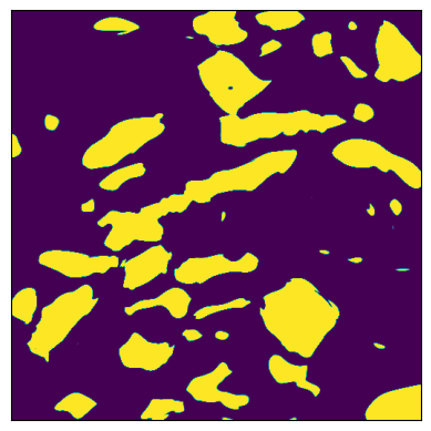
This section is concerned with computations on a two-dimensional slice of a $\mu$CT-scan of a wood-plastic composite (WPC) as shown in Figure 9(a). It consist of two phases, namely a polymer matrix phase and a wood short fiber inclusion phase. A $\mu$CT-scan yields a voxelized greyscale image, typically noisy. The noise from the imaging process was smoothed out by an Gaussian filter, followed by binarization to yield a voxelized representation of the two-phase material.

6.1 Material network

Unlike in the case of a single inclusion as seen in Section 4.3.2, for real-world microstructures an analytical description of the distribution of material parameters almost never exists. For more complex distributions we therefore propose the usage of an ANN, a material network, which learns the underlying microstructure in a supervised manner. A densely connected ANN from Section 3.1 is trained on the microstructure, such that

$$\left(\lambda(\bm{x}),\mu(\bm{x})\right)\approx\mathcal{N}_{mat}(\bm{x};\bm{\theta}),$$ ((48))

whereas the activation function $\phi^{(n_{L})}$ in Eq. (16) of the last layer $\bm{h}^{(n_{L})}$ is defined in the case of $\lambda(\bm{x})$ as

$$\phi^{(n_{L})}(\bm{x})=\left(\operatorname{tanh}(\phi^{(n_{L}-1)}(\bm{x}))+1\right)\frac{\lambda_{max}-\lambda_{min}}{2}+\lambda_{min},$$ ((49))

to only render physically admissible results. Here, $\lambda_{max}$ and $\lambda_{min}$ are the maximum and minimum values for $\lambda(\bm{x})$ in the domain $\Omega$ from Eq. (1). Eq. (49) is formulated similarly for $\mu(\bm{x})$. Therefore, the material network just learns to predict the correct material phase at a given spatial coordinate. During training, a pair consisting of a coordinate and the correct material phase is provided. As no generalization is needed, the training can be seen as a kind of overfitting to the spatial distribution of material phases. The resulting material network is a global, infinitely differentiable or smooth function for the given domain, which approximates the material distribution. The training usually only lasts several minutes. The resulting scalar fields then can be used within the PINN. This approach yields a smooth extension of the microstructure under consideration. In this work, an ANN with $n_{L}=20$ layers and $n_{u}=15$ units trained via BFGS yielded the best results. The material parameters $\lambda(\bm{x})$ and $\mu(\bm{x})$ are chosen as in Section 4.3.2.

A prediction of the material distribution of the $\mu$CT-scan in Figure 9(a) is shown in Figure 9(b).

(a) $\mu$CT-scan

(b) material network

Figure 9: Microstructure of WPC. (a) shows the $\mu$CT-scan after Gaussian filtering and binarization. (b) shows the smooth extension of the microstructure by the material network described in Section 6.1.

6.2 Numerical experiments

The numerical experiment investigating the $\mu$CT-scan in Figure 9 use the same boundary conditions described in Section 4.3.1 and shown in Figure 3. The material distribution and therefore the distribution of material parameters $\lambda(\bm{x})$ and $\mu(\bm{x})$ from Eq. (8) is provided by the material network described in Section 6.1.

6.2.1 Domain split - cPINN

First, the cPINN approach described in Section 5.2 is investigated with respect to the optimal domain splitting. To this end, several cPINNs with different number $N$ of domain splits $\Omega_{i}$ from Eq. (40), but roughly the same amount of parameters $\bm{\theta}$ from Eq. (19) $\bm{\theta}\approx 13\times 10^{3}$, resulting from $n_{L}=4$ layers $\bm{h}^{(l)}$ with the appropriate amount of neural units $h^{(l)}_{\eta}$ from Eq. (15), are trained for $1\times 10^{4}$ iterations. The results can be seen in Figure 10. It can be observed, that the mean of $\mathcal{R}$, the sum of the absolute residuals described in Section 4.3.1, is lower for increased number of domain splits and therefore, with increased number of ANNs, as described in Section 5.2. This is explained by the successive localization of the underlying BVP problem. On the other hand, more loss terms are added to the optimization problem in Section 5.2, which renders the optimization more difficult. This becomes clear in the error jump from the 4x4 split to the 5x5 split in Figure 10. Here, the number of ANNs used raises from 16 to 25 ANNs, a 36% increase, where for every additional ANN the loss term in Section 5.2 is expanded by the ANNs individual loss terms and interface conditions. Therefore, the 4x4 split yields the maximum number of ANNs for the localization advantage to outweigh the complexity gain in the loss. The 4x4 cPINN has a 25% lower mean residual $\mathcal{R}$ compared to the 1x1 split, which corresponds to the standard PINN approach.

Figure 10: Domain split - cPINN: Comparison of different domain splits from Eq. (40) of the cPINN approach described in Section 5.2, whereas 1x1 equals the standard PINN approach from Section 4. The splits are plotted against the mean of $\mathcal{R}$, the sum of the absolute residuals described in Section 4.3.1. The 4x4 cPINN has a 25% lower mean residual than the PINN approach.

6.2.2 $\mu$CT-scan - cPINN

Finally, the $\mu$CT-scan is recalculated using the 4x4 cPINN with $n_{L}=4$ and $n_{u}=90$, resulting in $\bm{\theta}\approx 2.7\times 10^{4}$ ANN parameters from Eq. (19). The training as well as the prediction is carried out on a regular grid consisting of $n_{d}=256^{2}$ collocation points. A maximum of $2\times 10^{4}$ iterations is used. The results are shown in Figure 11. The maximum of the residual residual $\mathcal{R}$ from Section 4.3.1 is $max(\mathcal{R})=9.249407$, the mean $\mathbb{E}(\mathcal{R})=1.20354064\times 10^{-1}$ and the minimum $min(\mathcal{R})=3.2151486\times 10^{-3}$. The L2-norm of the work balance loss from Eq. (29) is $||{\mathcal{L}_{W}}||=1.682084\times 10^{-2}$. Clearly, the proposed approach is able to resolve the local tensor, vector and scalar fields of interest, namely the stress tensor field $\bm{\sigma}(\bm{x})$, the displacement vector field $\bm{u}(\bm{x})$ as well as the point wise internal work $W_{int}(\bm{x})$. Again, the overall error $\mathcal{R}$ is highest at the boundaries of the inclusions. Comparing the residual field $\mathcal{R}$ in Figure 11 with the distribution of the material in Figure 9, conformity can be observed, as the boundaries of the material coincide with the highest error contours. Even small details are captured. In addition, minor incompatibilities occur at the subdomain interfaces.

Figure 11: $\bm{\mu}$CT-scan - cPINN: The resulting components of the stress tensor field $\bm{\sigma}(\bm{x})$ and displacement vector field $\bm{u}(\bm{x})$ as well as the point wise internal work $W_{int}$ for the microstructure from Section 6 using cPINNs as described in Section 5.2, in the top rows. In the bottom rows the absolute sum of the residuals $\mathcal{R}$ as well as the single residuals for the balance law $\mathcal{R}_{\nabla}^{\bullet}$ and the constitutive law $\mathcal{R}_{const}^{\bullet}$, as described in Section 4.3.1, are shown. The L2-norm of the work balance loss from Eq. (29) is $||{\mathcal{L}_{W}}||=1.6820842\times 10^{-2}$. Maximum number of iterations were $2\times 10^{4}$.

7 Conclusion and outlook

The objective of this paper is an in-depth study of a physics informed neural network approach for the solution of the governing equations of linear elastic continuum micromechanics without the need for training data. PINNs are an alternative to local numerical methods like FEM. Additionally, our approach works directly with the strong form of the elastostatics equations, rendering a global solution of the underlying BVP.

The unique challenges lie in the complex physical objects under consideration, namely nonlinear tensor fields, which arise due to the heterogeneous material distribution in the domain. The resulting governing equations, the balance law, the constitutive equation as well as the kinematic relation, inherit tensor fields of different scales as well as second order derivatives, rendering direct optimization difficult. The steep phase transition between different materials imposes a challenge on gradient based optimization.

In order to overcome these difficulties, a multi-output physics informed neural network is employed proposed at [25]. The PINN outputs stress as well as displacement fields, thereby circumventing the need for second order derivatives. An appropriate loss scaling for the optimization function is proposed, to overcome the problem of multi-scale loss components, enabling the PINN to tackle arbitrary material parameter combinations. Boundary conditions of the BVP are implicitly fulfilled by means of hard boundary conditions, thus simplifying the loss function and rendering the optimization process more simple. Furthermore, using hard boundary conditions allows to use smaller ANNs, which can focus solely on the interior solution fields inside the domain of interest. The optimization itself is carried out using the BFGS algorithm, which is computationally feasible due to the small ANN used, yielding faster convergence rates than ADAM or L-BFGS. To further accelerate the accuracy of the solution, the work balance of internal and external work is included to the overall loss, acting like a global constraint besides the point-wise residuals. Furthermore, an adaptive sampling method for the collocation points inside the domain is proposed. Additionally, a domain decomposition cPINN approach proposed in [49] is applied to elastostatics. To handle arbitrarily complex microstructures, a material network is employed, which yields a smooth extension of the underlying material parameter fields, simplifying the gradient descent optimization by circumventing gradient jumps.

Several numerical examples were given. The first example showed the accuracy of the standard PINN approach on a homogeneous plate. The BFGS optimizer was able to find appropriate weights for the PINN to yield state of the art precision. In a second experiment, the PINN approach was tested qualitatively on an inhomogeneous plate with a single inclusion. The PINN was able to qualitatively resolve the underlying tensorial fields. The highest errors appeared in the phase transition zone. To handle this problem, an adaptive collocation point sampling algorithm was tested. To further simplify the underlying BVP, a domain decomposition algorithm was introduced. Comparisons of the standard PINN, the cPINN and adaptive PINN and cPINN algorithms showed, that the cPINN approach using regular sampling yielded the highest accuracy. The adaptive algorithm seems to introduce difficulties for the optimization method used. While the performance was better for low numbers of collocation points, it disoriented for finer grids. Finally, the performance of cPINN on a real-world $\mu$CT-scan of WPC was investigated. Here it was shown, that there is an optimal number of domain splits, which rendered a trade-off between localization of the problem, thus simplifying the nonlinear solution fields, and the rising complexity of the loss function, thus complicating the optimization process. The cPINN was able to resolve the complex stress, displacement and energy fields.

It has been demonstrated that PINNs are able to solve nonlinear partial differential equations in the context of elastostatics with inhomogeneous parameters. This problem is challenging for PINNs which approximate the highly localized solution with a global ansatz. There are several potential applications for this approach. It was shown that PINNs due to the smoothness of their solutions and the formulation as an optimization problem are especially well suited for inverse problems, see e.g., [50] and [30]. In this context, the identification of sensor placement and optimal experimental design could benefit from the adaptive sampling approach presented in this work. Regarding the identification of material parameters, physical constraints could render semi-supervised learning possible. Usually, thousands of data points are needed for conventional supervised learning approaches. Using PINNs, the regularization by physical laws could reduce the amount of data needed to yield precise results. For forward problems, the presented PINN approach is not competitive compared to FEM or FFT based methods with respect to computational time, as for large problems the optimization can last several hours on GPUs. Here, FEM and FFT methods are more mature. On the other hand, for inverse problems, recent work in parameter identification of solids are promising [22]. In inverse problems for continuum mechanics, the loss is a function of the material parameters, the provided solution fields and the PDE. The work at hand shows that PINNs are able to resolve the complicated solutions present in heterogeneous problems. It is therefore a first step towards using the PINN approach for regularization of ANNs in inverse problems by means of the underlying, known physics, encoded in the PDEs. The development of PINN for inverse problems in the context of solid mechanics is ongoing work of the authors’ group [51].

Furthermore, towards forward problems, it is possible to include more physics into the ANN, e.g., more complex material laws or even aleatoric and epistemic uncertainty in the form of probability distributions or fuzzy methods [52]. Recent developments in parallel cPINNs [53] and Extended PINNs (XPINNs) [54] could leverage the applicability of PINNs to large, multi-scale problems. XPINNs could be an interesting extension to the cPINN approach to increase the accuracy in microstructural investigations. Here, the phase transition areas are captured by means of an indicator function. Parallel PINNs allow the simultaneous calculation of weight updates for multi-network architectures, making it possible to consider industry-scale problems.

To summarize, the proposed PINN and cPINN approaches are able to predict highly nonlinear tensorial fields in the context of continuum micromechanics. This work showed, that they are adequately able to capture the underlying complex physics of microstructural elastostatics. Their full potential is yet to be investigated, leaving room for further investigations such as uncertainty quantification and inverse problems.

References

- [1] S. David Müzel, E. P. Bonhin, N. M. Guimarães, E. S. Guidi, Application of the finite element method in the analysis of composite materials: A review, Polymers 12 (4) (2020) 818.
- [2] Y. LeCun, Y. Bengio, G. Hinton, Deep learning, nature 521 (7553) (2015) 436–444.
- [3] V. Lantz, N. Abiri, G. Carlsson, M.-E. Pistol, Deep learning for inverse problems in quantum mechanics, International Journal of Quantum Chemistry 121 (9) (2021) e26599.
- [4] S. Min, B. Lee, S. Yoon, Deep learning in bioinformatics, Briefings in bioinformatics 18 (5) (2017) 851–869.
- [5] F. Piccialli, V. Di Somma, F. Giampaolo, S. Cuomo, G. Fortino, A survey on deep learning in medicine: Why, how and when?, Information Fusion 66 (2021) 111–137.
- [6] L. Lu, P. Jin, G. Pang, Z. Zhang, G. E. Karniadakis, Learning nonlinear operators via deeponet based on the universal approximation theorem of operators, Nature Machine Intelligence 3 (3) (2021) 218–229.
- [7] F. E. Bock, R. C. Aydin, C. J. Cyron, N. Huber, S. R. Kalidindi, B. Klusemann, A review of the application of machine learning and data mining approaches in continuum materials mechanics, Frontiers in Materials 6 (2019) 110.
- [8] J. N. Kutz, Deep learning in fluid dynamics, Journal of Fluid Mechanics 814 (2017) 1–4.
- [9] Y.-C. Hsu, C.-H. Yu, M. J. Buehler, Using deep learning to predict fracture patterns in crystalline solids, Matter 3 (1) (2020) 197–211.
- [10] A. Henkes, I. Caylak, R. Mahnken, A deep learning driven pseudospectral PCE based FFT homogenization algorithm for complex microstructures, Computer Methods in Applied Mechanics and Engineering 385 (2021) 114070.
- [11] I. E. Lagaris, A. Likas, D. I. Fotiadis, Artificial neural networks for solving ordinary and partial differential equations, IEEE transactions on neural networks 9 (5) (1998) 987–1000.
- [12] M. Raissi, P. Perdikaris, G. E. Karniadakis, Physics-informed neural networks: A deep learning framework for solving forward and inverse problems involving nonlinear partial differential equations, Journal of Computational Physics 378 (2019) 686–707.
- [13] G. E. Karniadakis, I. G. Kevrekidis, L. Lu, P. Perdikaris, S. Wang, L. Yang, Physics-informed machine learning, Nature Reviews Physics (2021) 1–19.
- [14] C. Rackauckas, Y. Ma, J. Martensen, C. Warner, K. Zubov, R. Supekar, D. Skinner, A. Ramadhan, A. Edelman, Universal differential equations for scientific machine learning, arXiv preprint arXiv:2001.04385 (2020).
- [15] G. S. Misyris, A. Venzke, S. Chatzivasileiadis, Physics-informed neural networks for power systems, in: 2020 IEEE Power & Energy Society General Meeting (PESGM), IEEE, 2020, pp. 1–5.
- [16] W. Ji, W. Qiu, Z. Shi, S. Pan, S. Deng, Stiff-pinn: Physics-informed neural network for stiff chemical kinetics, arXiv preprint arXiv:2011.04520 (2020).
- [17] M. Raissi, A. Yazdani, G. E. Karniadakis, Hidden fluid mechanics: Learning velocity and pressure fields from flow visualizations, Science 367 (6481) (2020) 1026–1030.
- [18] Q. Zhu, Z. Liu, J. Yan, Machine learning for metal additive manufacturing: predicting temperature and melt pool fluid dynamics using physics-informed neural networks, Computational Mechanics 67 (2) (2021) 619–635.
- [19] H. Wessels, C. Weißenfels, P. Wriggers, The neural particle method–an updated Lagrangian physics informed neural network for computational fluid dynamics, Computer Methods in Applied Mechanics and Engineering 368 (2020) 113127.
- [20] S. Cai, Z. Mao, Z. Wang, M. Yin, G. E. Karniadakis, Physics-informed neural networks (pinns) for fluid mechanics: A review, arXiv preprint arXiv:2105.09506 (2021).
- [21] S. A. Niaki, E. Haghighat, T. Campbell, A. Poursartip, R. Vaziri, Physics-informed neural network for modelling the thermochemical curing process of composite-tool systems during manufacture, Computer Methods in Applied Mechanics and Engineering 384 (2021) 113959.
- [22] E. Zhang, M. Yin, G. E. Karniadakis, Physics-informed neural networks for nonhomogeneous material identification in elasticity imaging, arXiv preprint arXiv:2009.04525 (2020).
- [23] S. Cai, Z. Wang, S. Wang, P. Perdikaris, G. E. Karniadakis, Physics-informed neural networks for heat transfer problems, Journal of Heat Transfer 143 (6) (2021) 060801.
- [24] M. Vahab, E. Haghighat, M. Khaleghi, N. Khalili, A Physics Informed Neural Network Approach to Solution and Identification of Biharmonic Equations of Elasticity, arXiv preprint arXiv:2108.07243 (2021).
- [25] E. Haghighat, M. Raissi, A. Moure, H. Gomez, R. Juanes, A physics-informed deep learning framework for inversion and surrogate modeling in solid mechanics, Computer Methods in Applied Mechanics and Engineering 379 (2021) 113741.
- [26] C. Rao, H. Sun, Y. Liu, Physics-informed deep learning for incompressible laminar flows, Theoretical and Applied Mechanics Letters 10 (3) (2020) 207–212.
- [27] E. Samaniego, C. Anitescu, S. Goswami, V. M. Nguyen-Thanh, H. Guo, K. Hamdia, X. Zhuang, T. Rabczuk, An energy approach to the solution of partial differential equations in computational mechanics via machine learning: Concepts, implementation and applications, Computer Methods in Applied Mechanics and Engineering 362 (2020) 112790.
- [28] S. Kollmannsberger, D. D’Angella, M. Jokeit, L. Herrmann, Deep Energy Method, in: Deep Learning in Computational Mechanics, Springer, 2021, pp. 85–91.
- [29] M. Guo, E. Haghighat, An energy-based error bound of physics-informed neural network solutions in elasticity, arXiv preprint arXiv:2010.09088 (2020).
- [30] C.-T. Chen, G. X. Gu, Learning hidden elasticity with deep neural networks, Proceedings of the National Academy of Sciences 118 (31) (2021).
- [31] Y. Shin, J. Darbon, G. E. Karniadakis, On the convergence and generalization of physics informed neural networks, arXiv e-prints (2020) arXiv–2004.
- [32] V. M. Nguyen-Thanh, X. Zhuang, T. Rabczuk, A deep energy method for finite deformation hyperelasticity, European Journal of Mechanics-A/Solids 80 (2020) 103874.
- [33] S. Li, G. Wang, Introduction to micromechanics and nanomechanics, World Scientific Publishing Company, 2008.
- [34] K. Hornik, M. Stinchcombe, H. White, Multilayer feedforward networks are universal approximators, Neural networks 2 (5) (1989) 359–366.
- [35] C. M. Bishop, Pattern recognition and machine learning, springer, 2006.
- [36] I. Goodfellow, Y. Bengio, A. Courville, Y. Bengio, Deep learning, Vol. 1, MIT press Cambridge, 2016.
- [37] C. C. Aggarwal, et al., Neural networks and deep learning, Springer 10 (2018) 978–3.
- [38] A. Géron, Hands-on machine learning with Scikit-Learn, Keras, and TensorFlow: Concepts, tools, and techniques to build intelligent systems, O’Reilly Media, 2019.
- [39] F. Chollet, et al., Deep learning with Python, Vol. 361, Manning New York, 2018.
- [40] P. Ramachandran, B. Zoph, Q. V. Le, Searching for activation functions, arXiv preprint arXiv:1710.05941 (2017).
- [41] J. Berg, K. Nyström, A unified deep artificial neural network approach to partial differential equations in complex geometries, Neurocomputing 317 (2018) 28–41.
-
[42]
M. Abadi, A. Agarwal, P. Barham, E. Brevdo, Z. Chen, C. Citro, G. S. Corrado,
A. Davis, J. Dean, M. Devin, S. Ghemawat, I. Goodfellow, A. Harp, G. Irving,
M. Isard, Y. Jia, R. Jozefowicz, L. Kaiser, M. Kudlur, J. Levenberg,
D. Mané, R. Monga, S. Moore, D. Murray, C. Olah, M. Schuster, J. Shlens,
B. Steiner, I. Sutskever, K. Talwar, P. Tucker, V. Vanhoucke, V. Vasudevan,
F. Viégas, O. Vinyals, P. Warden, M. Wattenberg, M. Wicke, Y. Yu,
X. Zheng, Tensorflow: Large-Scale Machine
Learning on Heterogeneous Systems, software available from tensorflow.org
(2015).
URL https://www.tensorflow.org/ - [43] L. Sun, H. Gao, S. Pan, J.-X. Wang, Surrogate modeling for fluid flows based on physics-constrained deep learning without simulation data, Computer Methods in Applied Mechanics and Engineering 361 (2020) 112732.
- [44] S. Wang, Y. Teng, P. Perdikaris, Understanding and mitigating gradient pathologies in physics-informed neural networks, arXiv preprint arXiv:2001.04536 (2020).
- [45] S. Wang, X. Yu, P. Perdikaris, When and why pinns fail to train: A neural tangent kernel perspective, arXiv preprint arXiv:2007.14527 (2020).
- [46] R. Fletcher, Practical methods of optimization john wiley & sons, New York 80 (1987) 4.
- [47] C. L. Wight, J. Zhao, Solving Allen-Cahn and Cahn-Hilliard equations using the adaptive physics informed neural networks, arXiv preprint arXiv:2007.04542 (2020).
- [48] C. Szegedy, V. Vanhoucke, S. Ioffe, J. Shlens, Z. Wojna, Rethinking the inception architecture for computer vision, in: Proceedings of the IEEE conference on computer vision and pattern recognition, 2016, pp. 2818–2826.
- [49] A. D. Jagtap, E. Kharazmi, G. E. Karniadakis, Conservative physics-informed neural networks on discrete domains for conservation laws: Applications to forward and inverse problems, Computer Methods in Applied Mechanics and Engineering 365 (2020) 113028.
- [50] Y. Chen, L. Lu, G. E. Karniadakis, L. Dal Negro, Physics-informed neural networks for inverse problems in nano-optics and metamaterials, Optics express 28 (8) (2020) 11618–11633.
- [51] D. Anton, H. Wessels, Identification of material parameters from full-field displacement data using physics-informed neural networks, Researchgate Preprint (2021). doi:10.13140/RG.2.2.24558.89924.
- [52] J. N. Fuhg, N. Bouklas, On physics-informed data-driven isotropic and anisotropic constitutive models through probabilistic machine learning and space-filling sampling, arXiv preprint arXiv:2109.11028 (2021).
- [53] K. Shukla, A. D. Jagtap, G. E. Karniadakis, Parallel physics-informed neural networks via domain decomposition, arXiv preprint arXiv:2104.10013 (2021).
- [54] A. D. Jagtap, G. E. Karniadakis, Extended physics-informed neural networks (xpinns): A generalized space-time domain decomposition based deep learning framework for nonlinear partial differential equations, Communications in Computational Physics 28 (5) (2020) 2002–2041.