Gauge effects in bound-bound Rydberg-transition matrix elements

Abstract

Accurate data on electric-dipole transition matrix elements (EDTMs) for bound-bound Rydberg-atom transitions become increasingly important in science and technology. Here we compute radial EDTMs of rubidium using the length, velocity and acceleration gauges for electric-dipole-allowed transitions between states with principal and angular-momentum quantum numbers ranging from 15 to 100. Wave-functions are computed based upon model potentials from Marinescu et al., Phys. Rev. A 49, 982 (1994). Length-gauge EDTMs, often used for low-$\ell$ transitions, are found to deviate from the fundamentally more accurate velocity-gauge EDTMs by relative amounts of up to $\sim 10^{-3}$. We discuss the physical reasons for the observed gauge differences, explain the conditions for applicability of the velocity and length gauges for different transition series, and present a decision tree of how to choose EDTMs. Implications for contemporary Rydberg-atom applications are discussed.

I Introduction

Rydberg atoms Gallagher (2005) are an active field of modern physics with applications in precision measurements Hare et al. (1993); Jentschura et al. (2010); Ramos et al. (2017); Berl et al. (2020), molecular physics Shaffer et al. (2018); Fey et al. (2020), quantum control Thaicharoen et al. (2019); Cardman and Raithel (2020), field sensing Sedlacek et al. (2012); Holloway et al. (2014); Anderson et al. (2021, 2020), nonlinear quantum optics Chang et al. (2014); Liang et al. (2018); Cantu et al. (2020), and as a platform for quantum computing and simulations Saffman (2016); Browaeys and Lahaye (2020); Morgado and Whitlock (2021). Being at the core of several directions in fundamental research and emerging quantum technologies Adams et al. (2019), Rydberg transitions from low-lying states or other Rydberg atomic states require accurate calculations Safronova et al. (2004); Šibalić et al. (2017). Of particular interest are electric and magnetic multipole transition matrix elements Safronova and Safronova (2011), static and dynamic polaizabilities Safronova et al. (2004); Chen et al. (2015), and collisional and photo-ionization Dinneen et al. (1992); Markert et al. (2010); Viray et al. (2021); Cardman et al. (2021) cross-sections. Among the former, electric-dipole transition matrix elements (EDTMs) are the most important due to their wide usage Safronova et al. (2004).

A common framework for the computation of EDTMs between different bound Rydberg levels is based on model potentials Marinescu et al. (1994). In most cases, the computations are performed in the length gauge (LG) Bethe and Salpeter (2012); Friedrich (2017), also referred to as Babushkin gauge Papoulia et al. (2019). Another common form is the velocity gauge (VG). In addition, there exists an acceleration gauge (AG). Although quantum mechanics is gauge-invariant Bethe and Salpeter (2012); Sakurai and Napolitano (2017), different approximations and assumptions must be made to transform the expressions for EDTMs between different gauges, which can result in notable discrepancies in the final results Grant (1974); Fischer (2009). These are revealed in high-precision calculations and naturally raise the question which gauge should be used. This issue has been discussed in a range of research fields, including interaction of atoms and molecules with strong fields Leone et al. (1989); Cormier and Lambropoulos (1996); Bauer et al. (2005); Chen and Hu (2009); Han and Madsen (2010); Bandrauk et al. (2013), solid-state physics Virk and Sipe (2007); Passos et al. (2018) and astrophysical spectroscopy A. Pehlivan Rhodin et al. (2017); Papoulia et al. (2019).

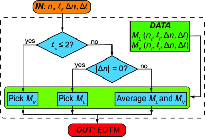
FIG. 1: Decision tree to select EDTMs from pre-computed length-gauge and velocity-gauge databases of EDTMs, $M_{L}(n_{i},\ell_{i},\Delta n,\Delta\ell)$ and $M_{V}(n_{i},\ell_{i},\Delta n,\Delta\ell)$, respectively. Initial- and final-state principal and angular-momentum quantum numbers are denoted $(n_{i},\ell_{i})$ and $(n_{f},\ell_{f})$, respectively, the difference $\Delta n=n_{f}-n_{i}$, the difference $\Delta\ell=\ell_{f}-\ell_{i}=\pm 1$, and $\ell_{<}$ is the lesser of $\ell_{i}$ and $\ell_{f}$.

To our knowledge, gauge effects in EDTMs have not been broadly discussed yet in context with emerging applications of Rydberg-atom transitions in the aforementioned quantum technologies. Here we provide a comparison of EDTMs computed in the LG, VG and AG gauges for electric-dipole electromagnetic transitions in rubidium Rydberg atoms. The main emphasis is placed on the LG and VG forms, the most widely used and the most accurate gauges, respectively, while the AG is discussed for instructive purposes. We show that the angular-momentum type of the Rydberg-Rydberg transition plays a decisive role in what is the best choice for the gauge that should be used. For the Rb model potentials Marinescu et al. (1994) that we use to compute the Rydberg-electron wave-functions, we find that the VG should be used if the lesser of the involved angular momenta, $\ell_{<}$, is 2 or lower, and that the VG or the LG can be used otherwise, as they produce identical results within the numerical accuracy level of the calculations. As an exception, only the LG should be used for transitions between near-degenerate Rydberg levels with $l_{<}\geq 3$. The decision tree that follows is summarized in Fig. 1 and is rationalized throughout the paper. While the AG should not be used in applications, for instructive purposes we show that the AG results converge with the VG and LG results in the appropriate limits.

The paper is organized as follows: The three gauge forms are reviewed and the relevant expressions are provided in Sec. II, the results are presented in Sec. III and discussed in Sec. IV. The paper in concluded in Sec. V.

II Matrix elements in different gauge forms

In this section, we review the formalism for calculations of EDTMs in the three gauges, and justify the validity of the electric-dipole approximation (EDA). We begin with a spin-less, non-relativistic $N$-electron atom with nuclear charge $Z$ placed in a plane-wave electromagnetic field. The linearly polarized field has a vector potential $\mathbf{A}({\bf{r}},t)={\bf{A}}_{0}\cos({\bf{k}}\cdot{\bf{r}}-\omega t)$, wavevector $\mathbf{k}$, angular frequency $\omega$, and an amplitude of the electric field of $E_{0}=\omega A_{0}$. The atom can be described by the following Hamiltonian:

$$\hat{H}=\hat{H}_{0}+\hat{H}_{int},$$ (1)

where the field-free part, $\hat{H}_{0}$, is (in SI units)

$$\hat{H}_{0}=\sum_{i=1}^{N}\left(\frac{\hat{\mathbf{p}}_{i}^{2}}{2m_{e}}-\frac{Ze^{2}}{4\pi\epsilon_{0}\hat{r}_{i}}\right)+\frac{1}{4\pi\epsilon_{0}}\sum_{\begin{subarray}{c}i=1\\ i\neq j\end{subarray}}^{N}\frac{e^{2}}{|\hat{\mathbf{r}}_{i}-\hat{\mathbf{r}}_{j}|},$$ (2)

and the atom-field interaction part, $\hat{H}_{int}$, resulting from including the kinetic momentum, $\hat{\mathbf{P}}_{i}=\hat{\mathbf{p}}_{i}+e\hat{\mathbf{A}}(\hat{\mathbf{r}}_{i},t)$, is

$$\begin{split}\hat{H}_{int}=\sum_{i=1}^{N}\Bigl{(}\frac{e}{2m_{e}}[\hat{\mathbf{p}}_{i}\cdot\mathbf{A}(\hat{\mathbf{r}}_{i},t)+\mathbf{A}(\hat{\mathbf{r}}_{i},t)\cdot\hat{\mathbf{p}}_{i}]\\ +\frac{e^{2}\mathbf{A}^{2}(\hat{\mathbf{r}}_{i},t)}{2m_{e}}\Bigr{)}.\end{split}$$ (3)

Here, $e$ is the magnitude of the electron charge, $m_{e}$ is the electron mass, and $\hat{\mathbf{r}}_{i}$ are the position operators of the electrons. The ${\bf{A}}^{2}$-term in Eq. 3 describes the ponderomotive interaction, which can be employed to realize ponderomotive optical lattices for Rydberg atoms Dutta et al. (2000); Anderson et al. (2011). In the present work, we focus on the first term, which describes, among other phenomena, Rydberg-atom microwave transitions.

We consider an alkali atom with a single electron excited to Rydberg state. The sum in Eq. 3 can be dropped, and the interactions of the Rydberg electron with the core electrons can be compounded into a set of $\ell$-specific model potentials Marinescu et al. (1994). Adopting the Coulomb gauge, $\nabla\cdot\mathbf{A}=0$, in which $\hat{\mathbf{p}}$ and $\mathbf{A}(\hat{\mathbf{r}}_{i})$ commute, and also dropping the $\mathbf{A}^{2}$-term, which is irrelevant for the low-field transitions considered here, Eq. 3 can be written as:

$$\hat{H}_{int}=\frac{e}{m_{e}}\mathbf{A}(\hat{\mathbf{r}})\cdot\hat{\mathbf{p}}.$$ (4)

We then express the electric-field-normalized atom-field interaction matrix element between initial, $\left|i\right\rangle$, and final, $\left|f\right\rangle$, states of the Rydberg atom, in the rotating-wave approximation, as:

$$M_{V}=\frac{\left\langle f\right|\hat{H}_{int}\left|i\right\rangle}{(E_{0}/2)}=-\frac{e\hbar}{{\rm{i}}m_{e}\omega}(\hat{\mathbf{n}}\cdot\int\psi_{f}^{*}e^{{\rm{i}}\mathbf{k}\cdot\mathbf{r}}\nabla\psi_{i}d^{3}r)\quad.$$

Making the electric-dipole approximation (EDA), which is valid for microwave transitions of Rydberg atoms and is addressed further below,

$$M_{V}=-\frac{e\hbar}{{\rm{i}}m_{e}\omega}(\hat{\mathbf{n}}\cdot\int\psi_{f}^{*}~{}\nabla\psi_{i}~{}d^{3}r),$$ (5)

where $\hat{\mathbf{n}}$ is the electric field’s polarization vector. The electric-dipole transition matrix element (EDTM) in Eq. 5 is commonly referred to as the velocity(VG)-form, as it essentially involves the linear-momentum operator. In order to transform it into the often-used length-gauge(LG) form, one invokes the commutation relation $[\hat{\mathbf{r}},\hat{H}_{0}]=\frac{i\hbar}{m_{e}}\hat{\mathbf{p}}$, which is exact only if $\hat{H}_{0}$ does not contain momentum-dependent potentials Bethe and Salpeter (2012). For the case of an on-resonant interaction, $\omega=|E_{f}-E_{i}|/\hbar$ with final- and initial-state energies $E_{f}$ and $E_{i}$, respectively, the EDTM takes the commonly employed LG form,

$$M_{L}=e(\hat{\mathbf{n}}\cdot\int\psi_{f}^{*}~{}\mathbf{r}~{}\psi_{i}~{}d^{3}r).$$ (6)

For our third, the acceleration-gauge (AG) form, to be valid, the valence-electron potential in $\hat{H}_{0}$ must be of pure Coulomb form, $\hat{V}=-Ze^{2}/(4\pi\epsilon_{0}\hat{r})$, such that the commutation relation $[\hat{\mathbf{p}},\hat{H}_{0}]=-i\hbar\nabla\hat{V}$ is true Bethe and Salpeter (2012). Then, the EDTM can be expressed in AG form,

$$M_{A}=-\frac{Ze^{3}}{m_{e}\omega^{2}}(\hat{\mathbf{n}}\cdot\int\psi_{f}^{*}~{}\frac{\hat{\mathbf{r}}}{4\pi\epsilon_{0}r^{3}}~{}\psi_{i}~{}d^{3}r).$$ (7)

Note that the EDTMs in Eqs. 5-7 are in SI units. In order to convert them to atomic units used in the next Section, one needs to divide by $ea_{0}$, where $a_{0}$ is the Bohr radius. (Alternately, set $\hbar=m_{e}=Z=e=4\pi\epsilon_{0}=1$ and convert $\omega$ from SI into atomic units.)

The VG is the most general form, whereas for the LG and AG to be applicable specific requirements must be satisfied. These always hold in the non-relativistic hydrogen atom. However, the alkali model potentials Marinescu et al. (1994), which we use here, are $\ell$-dependent for $\ell\leq 3$, which makes the LG inaccurate at these low $\ell$-values. Rydberg atoms with a polarizable ionic core, such as Rb and Cs, exhibit a long-range, non-Coulombic core polarization potential, the leading term of which scales as $-\alpha_{d}/(2r^{4})$. There, $\alpha_{d}$ is the dipolar core polarizability. Due to the non-Coulombic perturbation, the AG is inaccurate at most $\ell$-values. It is an objective of our work to quantify the deviations of EDTMs computed in the LG and the marginally applicable AG forms from those computed in the fundamentally accurate VG form.

It is noteworthy that the EDA must be applied to the VG, the fundamental gauge that follows directly from the ${\bf{A}}\cdot{\bf{p}}$-part of the minimal-coupling Hamiltonian in Eq. 4, before the matrix element can be transformed into the LG and AG forms (under the applicable respective conditions). For the microwave transitions considered in the present work, the EDA is naturally satisfied due to the long radiation wavelength (${\bf{k}}\cdot{\bf{r}}\ll 1$). It has been shown elsewhere that the EDA even applies to electric Rydberg-atom couplings in the UV wavelength range Cardman et al. (2021), where the Rydberg-atom size typically exceeds the wavelength (${\bf{k}}\cdot{\bf{r}}>1$).

In the numerical results presented in Sec. III, we show comparisons between the EDTMs in the three gauges for several selected angular-momentum channels. All EDTMs shown are radial parts; matrix elements for transitions with specific magnetic quantum numbers follow from multiplication with angular matrix elements provided, for instance, in Bethe and Salpeter (2012).

The fine structure of the Rydberg levels is ignored in our analysis, as it would primarily only add Clebsch-Gordon factors to the angular matrix elements. The gauge effects we focus on in our work result from the $\ell$-dependence and the non-Coulombic long-range terms in the model potentials Marinescu et al. (1994) used to compute the radial wave-functions of the $(n,\ell)$-states of the atom. To capture gauge effects, it is therefore sufficient to consider radial EDTMs with fine-structure-averaged quantum defects Gallagher (2005) for the Rydberg energy levels. As the model potentials vary if $\ell\in[0,3]$ and are identical if $\ell\geq 3$, for $\ell_{<}\leq 2$ we expect to find errors of both the LG and AG results relative to the VG result. The latter is considered correct within our model. For $\ell_{<}\geq 3$ we still expect to find errors of the AG result due to the non-Coulombic, long-range ion-core polarization potential.

For the numerical calculation of the required wave-functions, we use a method described in Reinhard et al. (2007) that allows a non-uniform spatial grid. The spatial finesse is essentially characterized by a specifiable number of grid points per local de-Broglie wavelength of the electron wave-function (which varies widely within the atomic potential). For the bulk of our calculations, we chose a lower limit of 5,000 grid points per electron wavelength. To estimate numerical uncertainty, several computation series were performed on finer grids with a minimum of 10,000 grid points per electron wavelength. All computations were performed in Fortran using REAL*16 precision. For reference, less than 500 grid points per electron wavelength, in a REAL*8 implementation, suffice to compute EDTMs of strong bound-bound Rydberg transitions with three to four significant digits.

III Results

We have computed the EDTMs in all three gauges for all electric-dipole-allowed Rydberg-Rydberg transitions $n_{i}\rightarrow n_{f}$, with initial, $n_{i}$, and final, $n_{f}$, principal quantum numbers covering the full range from 15 to 100, and for all combinations of initial and final angular momenta, $\ell_{i}$ and $\ell_{f}$, that satisfy the electric-dipole selection rule $\Delta\ell=\ell_{f}-\ell_{i}=\pm 1$. The results are stored in data banks $M_{V}(n_{i},\ell_{i},\Delta n,\Delta\ell)$, $M_{L}(n_{i},\ell_{i},\Delta n,\Delta\ell)$, and $M_{A}(n_{i},\ell_{i},\Delta n,\Delta\ell)$, with $\Delta n$ defined as $\Delta n=n_{f}-n_{i}$.

As a convenient measure for the differences between the radial EDTMs in the three gauges, we define the relative gauge error

$$\delta_{i,V}=\left|1-\frac{M_{i}}{M_{V}}\right|,i=L,A,$$

where the subscripts V, L and A stand for VG, LG and AG gauges, respectively.

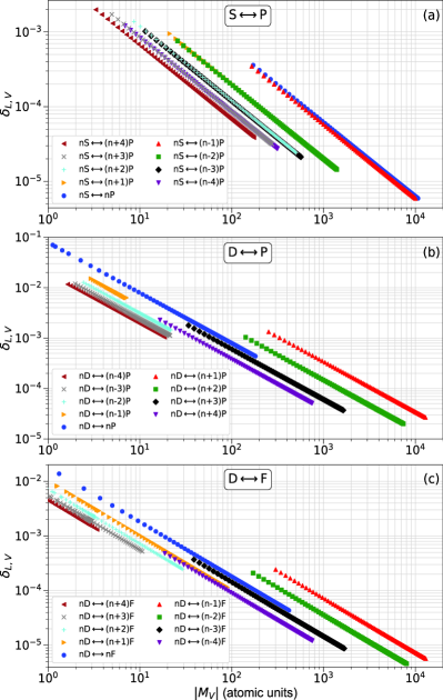
FIG. 2: (Color online) Comparison of EDTMs calculated in LG vs VG using Eqs. 5 and 6 for the indicated $n_{i}S\leftrightarrow n_{f}P$ series (a), $n_{i}D\leftrightarrow n_{f}P$ series (b), and $n_{i}D\leftrightarrow n_{f}F$ series (c).The principal quantum numbers $n$ range between 15 (left margin, in most series), and 100 (right margin, in most series).

In Fig. 2, we show $\delta_{L,V}$ vs $|M_{V}|$ on double-log scales for several transition series with $\ell_{<}\leq 2$. We consider transitions with $|\Delta n|\leq 4$, which include the series with the largest EDTMs (that are relevant in numerous applications). It is first noted that each series falls on a well-defined line characteristic to the series. All characteristic lines have similar slopes, with the distributions of data points $(|M_{V}|,\delta_{L,V})$ along those lines showing some irregularity for weak transitions (transitions with small $|M_{V}|$).

Rb $n_{i}S_{1/2}$ $\leftrightarrow$ $n_{f}P_{J}$ microwave transitions are of some importance because the $n_{i}S_{1/2}$ Rydberg atoms can be initialized by two-photon laser excitation from the Rb $5S_{1/2}$ ground state. As seen in Fig. 2(a), for the strongest transitions, $nS\leftrightarrow nP$ and $nS\leftrightarrow(n-1)P$, $\delta_{L,V}$ typically ranges between $10^{-4}$ and $10^{-5}$, while for the weaker transitions with larger $|\Delta n|$ this number can be as large as $\sim 2\times 10^{-3}$. Further, from the observed approximate scaling $\delta_{L,V}\propto 1/|M_{V}|$ it follows that $\Delta_{L,V}:=M_{L}-M_{V}$ tends to be a constant for each series. For the strongest series, $nS\leftrightarrow nP$ and $nS\leftrightarrow(n-1)P$, it is $\Delta_{L,V}\approx-0.062$ ea₀ and $-0.058$ ea₀, respectively. For the weaker series, the approximately constant values of $\Delta_{L,V}$ generally drop. For instance, for the $nS\leftrightarrow(n+4)P$ series it is $\Delta_{L,V}\approx-0.0066$ ea₀.

Rb $n_{i}D$ $\leftrightarrow$ $n_{f}P$ microwave transitions are often used because of the large values of $|M_{V}|$ on the $nD$ to $(n+1)P$ series, and because the two-photon laser preparation rates of $n_{i}D$ Rydberg atoms from the Rb $5S_{1/2}$ ground state are greater than those of $n_{i}S$ Rydberg atoms. It is seen in Fig. 2(b) that these transitions have $\delta_{L,V}$-values on the order of three times larger than those of comparable $n_{i}S$ $\leftrightarrow$ $n_{f}P$ transitions, with numerous instances of $\delta_{L,V}>10^{-2}$. On the $n_{i}D\leftrightarrow n_{f}P$ series, the $\delta_{L,V}$ are much larger and the $M_{V}$ much smaller for $\Delta n\leq 0$ than for $\Delta n>0$. The strongest series, $nD\leftrightarrow(n+1)P$, has $M_{L}-M_{V}\approx-0.34$ ea₀. Interestingly, the $nD\leftrightarrow nP$ series is very weak and exhibits a peculiar behavior at small $|M_{V}|$. We attribute the unusual features of the $nD\leftrightarrow nP$ series to the exact level energies and wave-functions of the involved states, which depend on the Rb quantum defects of both initial and final levels. In fact, further check revealed that this series exhibits what may be characterized as a bound-bound analog of a Cooper minimum Cooper (1962); Viray et al. (2021). (A Cooper minimum Cooper (1962) is a class of EDTM zeros at certain quantum-defect-dependent photo-ionization energies.) In the present case, the $nD\leftrightarrow nP$ EDTMs pass through a pronounced minimum of $|M_{V}|\sim 0.16$ ea₀ at $n=20$ (off-scale in Fig. 2(b)), which is about three orders of magnitude lower than the $|M_{V}|$-value of the nearby $20D\leftrightarrow 21P$ transition (which has $|M_{V}|=472$ ea₀). In Fig. 2(b), this results in an irregularity of the distribution of data points on the $nD\leftrightarrow nP$ series at low $|M_{V}|$. Since the relation $\delta_{L,V}\propto 1/|M_{V}|$ still holds, $\delta_{L,V}$ reaches as high as $\sim 0.5$ for the $20D\leftrightarrow 20P$ transition. Further examination reveals another unusual series, the $nD\leftrightarrow(n-1)P$ series. We found that in that case the EDTMs pass through a shallow maximum of $|M_{V}|$ of only $\approx 7$ ea₀ at $n\sim 65$. This maximum results in a “bunching” of data points in Fig. 2(b) at the right margin of the $nD\leftrightarrow(n-1)P$ series.

We further show several $n_{i}D\leftrightarrow n_{f}F$ series in Fig. 2(c). Figures 2(b) and 2(c) have some resemblance, which one may attribute to similar differences in the quantum defects of the respective involved states. In the $n_{i}D\leftrightarrow n_{f}F$ series, the $\delta_{L,V}$ are much larger and the $M_{V}$ much smaller for $\Delta n\geq 0$ than for $\Delta n<0$. Investigating further, we find that the $\Delta n\geq 0$ cases all show a Cooper-minimum-like behavior, similar to the $nD\leftrightarrow nP$ series in Fig. 2(b). In addition, the EDTMs of the $n_{i}D\leftrightarrow n_{f}F$ series with $\Delta n>0$ pass through maxima at series-dependent $n_{i}$-values located below the respective “Cooper-minima”. These effects result in irregular appearances of the distribution of data points on the $n_{i}D\leftrightarrow n_{f}F$ series with $\Delta n\geq 0$ in Fig. 2(c).

For $\ell\geq 3$, the utilized model potentials become $\ell$-independent, and numerical readings of $\delta_{L,V}\neq 0$ are only due to numerical error. For instance, for $n_{i}F\leftrightarrow n_{f}G$ transitions (not shown here) we find $\delta_{L,V}$-values peaking near $10^{-6}$. This indicates a relative numerical confidence level of the EDTMs below $\sim 10^{-5}$. This was verified by comparing several results from Fig. 2 with similar results obtained with a finer spatial grid in the wave-function calculations. This estimation of the numerical error is important because it shows that the deviations between $M_{L}$ and $M_{V}$, discussed in Figs. 2(a)-(c) and in the corresponding text passages above, are indeed due to the different gauge forms used.

Finally, we show a comparison between EDTMs computed in AG and VG. This comparison is of some fundamental interest but not relevant in applications of EDTMs. For low-$\ell$ states, $\delta_{A,V}$ can reach very large values (up to $\sim 10^{6}$, not shown here), reflecting the basic unsuitability of the AG for calculating EDTMs in non-Coulombic potentials. However, if $\ell$ becomes sufficiently large, the AG results tend to gradually approach the EDTMs calculated in VG and LG. As an example, in Fig. 3 we show results for several series for transitions between $\ell=10$ and $\ell=11$ states. On the series shown, the AG’s gauge error is small but it still exceeds the numerical error by several orders of magnitude. It is noteworthy that there is no apparent (simple) relationship between $\delta_{A,V}$ and $|M_{V}|$, and that $\delta_{A,V}$ increases with $|M_{V}|$. Both of these observations qualitatively differ from Fig. 2. In additional analyses, not presented, it is seen that $\delta_{A,V}$ drops below our numerical error for $\ell\gtrsim 20$ (with a caveat discussed in Sec. IV). This shows that the always-present error of the AG that is caused by the long-range ion-core polarization potential, $-\alpha_{d}/(2r^{4})$, drops below our present numerical error when $\ell\gtrsim 20$.

FIG. 3: (Color online) Comparison of EDTMs calculated in AG vs VG using Eqs. 5 and 7, respectively, for the indicated transition series with $\ell_{i/f}=10$ or 11, for which gauge errors in the AG calculation are still significant. The principal quantum number $n$ ranges between 15 (left) and 100 (right margins).

IV Discussion

In Sec. III we have established and quantified deviations between LG- and VG- computations of EDTMs for transitions that involve Rydberg levels with $\ell_{<}\leq 2$. These deviations are caused by the dependence of the utilized model potentials Marinescu et al. (1994) on $\ell$ for $\ell\leq 3$. For transitions with $\ell_{<}\geq 3$, the model potentials are identical, and the EDTMs in LG and VG agree within our numerical error of $\delta_{L,V}$ of $<10^{-5}$. The gauge error of the AG, caused by the long-range, non-Coulombic core polarization potential $-\alpha_{d}/(2r^{4})$, rapidly drops with increasing $\ell_{<}$ and becomes undetectable for $\ell_{<}\gtrsim 20$. Due to the ubiquitous use of low-$\ell$ Rb Rydberg states in science and technology, the following discussion is focused on aspects of the gauge errors of the LG pertaining to low-$\ell$ states.

For the strongest transitions within the $\ell_{<}\leq 2$-series displayed in Fig. 2, the choice of the gauge form does not play an overwhelming role, as $\delta_{L,V}$ - the relative EDTM error incurred by adopting the LG instead of the VG - barely exceeds $10^{-3}$ even in the worst cases. Picking $n_{i}=40$ as a specific example, we find $\delta_{L,V}=4.0\times 10^{-5}$ for the strongest $S\leftrightarrow P$ transitions, $\delta_{L,V}=1.7\times 10^{-4}$ for the $40D\leftrightarrow 41P$ transition, and $\delta_{L,V}=3.6\times 10^{-5}$ for the $40D\leftrightarrow 39F$ transition. In high-precision spectroscopy, it would be fairly challenging to probe Rabi-frequency discrepancies at that level of precision (and to even calibrate RF electric fields with sufficient accuracy to enable such measurements). However, the weak $n_{i}P\leftrightarrow n_{f}D$ series and several of the $n_{i}D\leftrightarrow n_{f}F$ series have $\delta_{L,V}$-values in the 1$\%$-and-above range and exhibit several unusual behaviors, including Cooper-minimum-like features. The properties of these weak series may offer opportunities to explore gauge effects in Rydberg electric-dipole transitions for fundamental investigations. The same holds for photo-ionization cross sections, which generally show larger differences between LG and VG Viray et al. (2021); Cardman et al. (2021) than bound-bound EDTMs.

It is abundantly evident in Fig. 2 that all data points for any given series that involves $\ell$-dependent model potentials fall on approximately straight lines, regardless of any added complexity such as Cooper-like minima in $|M_{V}|$. Fitted slopes are $\approx-1$ for all three types of transitions in Fig. 2. This observation implies that the absolute difference in EDTMs, $\Delta_{L,V}=M_{L}-M_{V}$, remains constant over a wide range of $n$. In all series presented in Fig. 2, the relative variation of $\Delta_{L,V}$ across the entire series is less than 2$\%$. Further investigation might be needed to explain this finding. The value of $\Delta_{L,V}$ is largest for the strongest series, $nD\leftrightarrow(n+1)P$, at $\Delta_{L,V}=-0.34$ ea₀.

The $1/\omega^{2}$-dependence of $M_{A}$ (see Eq. 7) and the $1/\omega$-dependence of $M_{V}$ (see Eq. 5) cause an issue of numerical accuracy for near-degenerate transitions. The integral expressions in the respective equations can drop to near or even below the numerical error. As a result, for near-degenerate transitions the expressions in Eqs. 5 and 7 can become numerically unstable and lead to non-physical results. (This is why in Fig. 3 we have excluded the result for $\Delta n=0$.) Since the LG (Eq. 6) has no equivalent numerical problem, the frequency-denominator issue is of no practical concern. For $\ell_{<}\leq 2$, where the VG must be used, there are no near-degenerate transitions, so the issue does not arise, while for $\ell_{<}\geq 3$, where near-degenerate transitions occur when $\Delta n=0$, the LG may be used.

Following the discussion, we are using the method summarized in Fig. 1 to pick EDMTs for any electric-dipole transition of interest. First, we compute databases $M_{V}(n_{i},l_{i},\Delta n,\Delta_{\ell})$, $M_{L}(n_{i},l_{i},\Delta n,\Delta_{\ell})$ and $M_{A}(n_{i},l_{i},\Delta n,\Delta\ell)$. (The database $M_{A}$ is for added insight only.) After entering the transition labels $(n_{i},l_{i},\Delta n,\Delta\ell)$, the following simple rules are applied:

• If $\ell_{<}\leq 2$, pick $M_{V}(n_{i},l_{i},\Delta n,\Delta\ell)$.

• If $\ell_{<}\geq 3$ and $|\Delta n|\geq 1$, use the average of $M_{V}(n_{i},l_{i},\Delta n,\Delta\ell)$ and $M_{L}(n_{i},l_{i},\Delta n,\Delta\ell)$.

• If $\ell_{<}\geq 3$ and $|\Delta n|=0$, pick $M_{L}(n_{i},l_{i},\Delta n=0,\Delta\ell)$.

V Conclusion

We have presented results for EDTMs calculated in three different gauge forms: velocity, length and acceleration. Based on the analysis of the observed differences between these forms, we outlined a method for choosing the most appropriate gauge, depending on the quantum numbers of the transition. We have discussed aspects of the underlying physics. In the computations we have used model potentials for Rb from Marinescu et al. (1994). Analogous computations could be performed for cesium or other alkali atoms for which there is a set of model potentials.

The observed differences between the forms have negligible or only minor consequences in applications of Rydberg atoms for microwave field sensing Sedlacek et al. (2012); Holloway et al. (2014); Anderson et al. (2021, 2020), where strong transitions are used. For these, the relative effect of gauge on the EDTMs, $\delta_{L,V}$, remains below $\sim 10^{-3}$. Gauge effects with a significance $>1\%$ may be detectable in weak Rydberg-Rydberg transitions, which one may study to experimentally explore gauge effects.

It is finally noted that the DC Stark effect occurs at $\omega=0$, while the present work deals with resonant transitions at frequencies that are typically in the radio-frequency and microwave ranges. A limiting case of $\omega\rightarrow 0$, covered in our work, occurs for near-degenerate $\Delta n=0$ transitions between high-$\ell$ states. The limit $\omega\rightarrow 0$ requires caution because of the rise of Bloch-Siegert shifts caused by the counter-rotating terms Berman and Malinovsky (2010), which we have dropped early-on when making the rotating-wave approximation, and because of other complications. The limit $\omega\rightarrow 0$ may be treated better as a quasi-static DC Stark effect in a slowly-varying electric field. In that approach, no resonance condition is assumed and the static atom-field interaction operator $e{\bf{E}}\cdot\hat{\bf{r}}$ applies, for which the length-gauge EDTMs are exact. Hence, the (quasi-static) DC quadratic Stark effect of low-$\ell$ atomic states requires the length-gauge form of the EDTMs, (even at low $\ell$), whereas interactions with microwave electric fields involving the same low-$\ell$ states require the velocity-gauge form. This difference may become relevant in precision measurements of resonant AC versus DC electric fields as well as applications of Rydberg atoms in defining voltage standards Holloway et al. (2021).

References

- Gallagher (2005) T. F. Gallagher, Rydberg Atoms, Vol. 3 (Cambridge University Press, 2005).
- Hare et al. (1993) J. Hare, A. Nussenzweig, C. Gabbanini, M. Weidemuller, P. Goy, M. Gross, and S. Haroche, “Toward a Rydberg constant measurement on circular atoms,” IEEE Trans. Instr. Meas. 42, 331–334 (1993).
- Jentschura et al. (2010) U. D. Jentschura, P. J. Mohr, and J. N. Tan, “Fundamental constants and tests of theory in Rydberg states of one-electron ions,” J. Phys. B 43, 074002 (2010).
- Ramos et al. (2017) A. Ramos, K. Moore, and G. Raithel, “Measuring the Rydberg constant using circular Rydberg atoms in an intensity-modulated optical lattice,” Phys. Rev. A 96, 032513 (2017).
- Berl et al. (2020) S. J. Berl, C. A. Sackett, T. F. Gallagher, and J. Nunkaew, “Core polarizability of rubidium using spectroscopy of the to Rydberg transitions,” Phys. Rev. A 102, 062818 (2020).
- Shaffer et al. (2018) J. P. Shaffer, S. T. Rittenhouse, and H. R. Sadeghpour, “Ultracold Rydberg molecules,” Nat. Comm. 9, 1965 (2018).
- Fey et al. (2020) C. Fey, F. Hummel, and P. Schmelcher, “Ultralong-range Rydberg molecules,” Mol. Phys. 118, e1679401 (2020).
- Thaicharoen et al. (2019) N. Thaicharoen, K.R. Moore, D.A. Anderson, R.C. Powel, E. Peterson, and G. Raithel, “Electromagnetically induced transparency, absorption, and microwave-field sensing in a Rb vapor cell with a three-color all-infrared laser system,” Phys. Rev. A 100, 063427 (2019).
- Cardman and Raithel (2020) R. Cardman and G. Raithel, “Circularizing Rydberg atoms with time-dependent optical traps,” Phys. Rev. A 101, 013434 (2020).
- Sedlacek et al. (2012) J. A. Sedlacek, A. Schwettmann, H. Kübler, R. Löw, T. Pfau, and J. P. Shaffer, “Microwave electrometry with Rydberg atoms in a vapour cell using bright atomic resonances,” Nat. Phys. 8, 819–824 (2012).
- Holloway et al. (2014) C. L. Holloway, J. A. Gordon, S. Jefferts, A. Schwarzkopf, D. A. Anderson, S. A. Miller, N. Thaicharoen, and G. Raithel, “Broadband Rydberg atom-based electric-field probe for SI-traceable, self-calibrated measurements,” IEEE Trans. Antennas Propag. 62, 6169–6182 (2014).
- Anderson et al. (2021) D. A. Anderson, R. E. Sapiro, and G. Raithel, “A self-calibrated SI-traceable Rydberg atom-based radio frequency electric field probe and measurement instrument,” IEEE Trans. Antennas Propag. 69, 5931–5941 (2021).
- Anderson et al. (2020) D. A. Anderson, R. E. Sapiro, and G. Raithel, “Rydberg atoms for radio-frequency communications and sensing: Atomic receivers for pulsed rf field and phase detection,” IEEE Aerosp. Electron. Syst. Mag. 35, 48–56 (2020).
- Chang et al. (2014) D. E. Chang, V. Vuletić, and M. D. Lukin, “Quantum nonlinear optics — photon by photon,” Nat. Photonics 8, 685–694 (2014).
- Liang et al. (2018) Q.-Y. Liang, A. V. Venkatramani, S. H. Cantu, T. L. Nicholson, M. J. Gullans, A. V. Gorshkov, J. D. Thompson, C. Chin, M. D. Lukin, and V. Vuletić, “Observation of three-photon bound states in a quantum nonlinear medium,” Science 359, 783–786 (2018).
- Cantu et al. (2020) S. H. Cantu, A. V. Venkatramani, W. Xu, L. Zhou, B. Jelenković, M. D. Lukin, and V. Vuletić, “Repulsive photons in a quantum nonlinear medium,” Nat. Phys. 16, 921–925 (2020).
- Saffman (2016) M. Saffman, “Quantum computing with atomic qubits and Rydberg interactions: progress and challenges,” J. Phys. B 49, 202001 (2016).
- Browaeys and Lahaye (2020) A. Browaeys and T. Lahaye, “Many-body physics with individually controlled Rydberg atoms,” Nat. Phys. 16, 132–142 (2020).
- Morgado and Whitlock (2021) M. Morgado and S. Whitlock, “Quantum simulation and computing with Rydberg-interacting qubits,” AVS Quantum Science 3, 023501 (2021).
- Adams et al. (2019) C. S. Adams, J. D. Pritchard, and J. P. Shaffer, “Rydberg atom quantum technologies,” J. Phys. B 53, 012002 (2019).
- Safronova et al. (2004) M. S. Safronova, C. J. Williams, and C. W. Clark, “Relativistic many-body calculations of electric-dipole matrix elements, lifetimes, and polarizabilities in rubidium,” Phys. Rev. A 69, 022509 (2004).
- Šibalić et al. (2017) N. Šibalić, J. D. Pritchard, C. S. Adams, and K. J. Weatherill, “ARC: An open-source library for calculating properties of alkali Rydberg atoms,” Comput. Phys. Commun. 220, 319–331 (2017).
- Safronova and Safronova (2011) M. S. Safronova and U. I. Safronova, “Critically evaluated theoretical energies, lifetimes, hyperfine constants, and multipole polarizabilities in ,” Phys. Rev. A 83, 052508 (2011).
- Chen et al. (2015) Y.-J. Chen, L. F. Gonçalves, and G. Raithel, “Measurement of Rb scalar and tensor polarizabilities in a 1064-nm light field,” Phys. Rev. A 92, 060501(R) (2015).
- Dinneen et al. (1992) T. P. Dinneen, C. D. Wallace, K.-Y. N. Tan, and P. L. Gould, “Use of trapped atoms to measure absolute photoionization cross sections,” Opt. Lett. 17, 1706–1708 (1992).
- Markert et al. (2010) F. Markert, P. Würtz, A. Koglbauer, T. Gericke, A. Vogler, and H. Ott, “ac-Stark shift and photoionization of Rydberg atoms in an optical dipole trap,” New J. Phys. 12, 113003 (2010).
- Viray et al. (2021) M. A. Viray, E. Paradis, and G. Raithel, “Photoionization of nS and nD Rydberg atoms of Rb and Cs from the near-infrared to the ultraviolet spectral region,” New J. Phys. 23, 063022 (2021).
- Cardman et al. (2021) R. Cardman, J. L. MacLennan, S. E. Anderson, Y.-J. Chen, and G. Raithel, “Photoionization of Rydberg atoms in optical lattices,” New J. Phys. 23, 063074 (2021).
- Marinescu et al. (1994) M. Marinescu, H. R. Sadeghpour, and A. Dalgarno, “Dispersion coefficients for alkali-metal dimers,” Phys. Rev. A 49, 982–988 (1994).
- Bethe and Salpeter (2012) H. A. Bethe and E. E. Salpeter, Quantum Mechanics of One- and Two-Electron Atoms (Springer Science & Business Media, 2012).
- Friedrich (2017) H. Friedrich, Theoretical Atomic Physics (Springer International Publishing, 2017).
- Papoulia et al. (2019) A. Papoulia, J. Ekman, G. Gaigalas, M. Godefroid, S. Gustafsson, H. Hartman, W. Li, L. Radžiūtė, P. Rynkun, S. Schiffmann, K. Wang, and P. Jönsson, “Coulomb (velocity) gauge recommended in multiconfiguration calculations of transition data involving Rydberg series,” Atoms 7 (2019), 10.3390/atoms7040106.
- Sakurai and Napolitano (2017) J. J. Sakurai and J. Napolitano, Modern Quantum Mechanics, 2nd ed. (Cambridge University Press, 2017).
- Grant (1974) I. P. Grant, “Gauge invariance and relativistic radiative transitions,” J. Phys. B 7, 1458–1475 (1974).
- Fischer (2009) C. Froese Fischer, “Evaluating the accuracy of theoretical transition data,” Phys. Scr. T134, 014019 (2009).
- Leone et al. (1989) C. Leone, S. Bivona, R. Burlon, F. Morales, and G. Ferrante, “Gauge aspects in multichannel multiphoton ionization,” Phys. Rev. A 40, 1828–1837 (1989).
- Cormier and Lambropoulos (1996) E. Cormier and P. Lambropoulos, “Optimal gauge and gauge invariance in non-perturbative time-dependent calculation of above-threshold ionization,” J. Phys. B 29, 1667–1680 (1996).
- Bauer et al. (2005) D. Bauer, D. B. Milošević, and W. Becker, “Strong-field approximation for intense-laser–atom processes: The choice of gauge,” Phys. Rev. A 72, 023415 (2005).
- Chen and Hu (2009) Y. J. Chen and B. Hu, “Strong-field approximation for diatomic molecules: Comparison between the length gauge and the velocity gauge,” Phys. Rev. A 80, 033408 (2009).
- Han and Madsen (2010) Y.-C. Han and L. B. Madsen, “Comparison between length and velocity gauges in quantum simulations of high-order harmonic generation,” Phys. Rev. A 81, 063430 (2010).
- Bandrauk et al. (2013) A. D. Bandrauk, F. Fillion-Gourdeau, and E. Lorin, “Atoms and molecules in intense laser fields: gauge invariance of theory and models,” J. Phys. B 46, 153001 (2013).
- Virk and Sipe (2007) K. S. Virk and J. E. Sipe, “Semiconductor optics in length gauge: A general numerical approach,” Phys. Rev. B 76, 035213 (2007).
- Passos et al. (2018) D. J. Passos, G. B. Ventura, J. M. Viana Parente Lopes, J. M. B. Lopes dos Santos, and N. M. R. Peres, “Nonlinear optical responses of crystalline systems: Results from a velocity gauge analysis,” Phys. Rev. B 97, 235446 (2018).
- A. Pehlivan Rhodin et al. (2017) A. Pehlivan Rhodin, H. Hartman, H. Nilsson, and P. Jönsson, “Experimental and theoretical oscillator strengths of Mg I for accurate abundance analysis,” Astron. Astrophys. 598, A102 (2017).
- Dutta et al. (2000) S. K. Dutta, J. R. Guest, D. Feldbaum, A. Walz-Flannigan, and G. Raithel, “Ponderomotive optical lattice for Rydberg atoms,” Phys. Rev. Lett. 85, 5551–5554 (2000).
- Anderson et al. (2011) S. E. Anderson, K. C. Younge, and G. Raithel, “Trapping Rydberg atoms in an optical lattice,” Phys. Rev. Lett. 107, 263001 (2011).
- Reinhard et al. (2007) A. Reinhard, T. Cubel Liebisch, B. Knuffman, and G. Raithel, “Level shifts of rubidium Rydberg states due to binary interactions,” Phys. Rev. A 75, 032712 (2007).
- Cooper (1962) J. W. Cooper, “Photoionization from outer atomic subshells. A model study,” Phys. Rev. 128, 681–693 (1962).
- Berman and Malinovsky (2010) P. Berman and V. Malinovsky, Principles of Laser Spectroscopy and Quantum Optics (Princeton University Press, 2010).
- Holloway et al. (2021) C. L. Holloway, N. Prajapati, J. Kitching, J. A. Sherman, C. Teale, A. Rufenacht, A. B. Artusio-Glimpse, M. T. Simons, A. K. Robinson, and E. B. Norrgard, “Electromagnetically induced transparency based Rydberg-atom sensor for quantum-based voltage measurements,” (2021), arXiv:2110.02335 [physics.atom-ph] .